Solving Nonlinear Absolute Value Equations

Aris Daniilidis, Mounir Haddou, Trí Minh Lê, Olivier Ley

Abstract. In this work we show that several problems naturally modeled as Nonlinear Absolute Value Equations (NAVE), can be restated as Nonlinear Complementarity Problems (NCP) and solved efficiently using smoothing regularizing techniques under mild assumptions. Applications include ridge optimization and resolution of nonlinear ordinary differential equations.

Keywords: Nonlinear Absolute Value Equality, Complementarity problem, $P_{0}$-map, Numerical methods

AMS Classification: Primary: 90C33, 65K10 ; Secondary: 15B48, 65K15, 90C59.

1 Introduction

The last two decades, absolute value equation problems (in short, AVE problems) have been extensively studied in the literature. This interest is justified by the fact that this class of problems already covers a wide spectrum of applications: indeed, numerous problems stemming from real-life applications, as for instance all mixed integer linear programming problems, can be reformulated as AVE problems. It is also well-known, see [32, 24] e.g., that AVE problems admit an equivalent description as Linear Complementarity problems (in short, LCP). The exact definitions of an AVE problem and a LCP are recalled below. Dealing efficiently with these problems is thus paramount.
The literature on this subject contains several theoretical results for existence as well as conditions guaranteeing uniqueness of the solution [23, 35, 34, 22]. Concurrently, there are also various numerical approaches to solve an AVE problem. Generally speaking, these methods can be divided into at least three categories [3] : iterative linear algebra based methods (also known as projective methods), semi-smooth Newton-like methods and smoothing methods. The aforementioned methods generally require some assumption on the matrix involved in the AVE problem. In particular, the classes of $P_{0}$-matrices and $P$-matrices (recalled below) turn out to be particularly relevant in this study [1].
In this work, we consider a natural generalization of (linear) AVE problems to nonlinear ones, known as Nonlinear Absolute Value Equations (in short, NAVE). This more general framework encompasses new applications including ridge regression models, bounded constrained nonlinear systems of equations, and stiff Ordinary Differential Equations (in short, stiff ODE). This approach to deal with the aforementioned problems, based on NAVE, is to the best of our knowledge, completely new in the literature.
Our main contribution is the following: we first show that similarly to the way that an AVE problem is linked to a LCP, nonlinear absolute value equations can also be associated to nonlinear complementarity problems (in short, NCP). Indeed, any NCP can be reformulated as NAVE. The converse is also true, but the association is generally given in an implicit way. Then, taking profit from the huge literature concerning existence, uniqueness and numerical resolution of NCP (see [9, 23, 35, 37] e.g.), we propose a new method to solve a NAVE problem, based on the smoothing technique proposed in [10] and further developments in the follow-up work [30]. The proposed approach is explained in Section 2, while in Section 3 we discuss applications.
To ease the reading we start with some definitions and settings. The Absolute Value Equality problem (in short, AVE) is defined as follows:

$$\text{find }x\in\mathbb{R}^{d}:\qquad Ax-|x|=b,$$ (AVE)

where $A$ is a $(d\times d)$-matrix and $b\in\mathbb{R}^{d}$. Throughout this work, given $x=(x^{1},\ldots,x^{d})^{T}\in\mathbb{R}^{d}$, we use the notation $|x|:=(|x^{1}|,\ldots,|x^{d}|)^{T}$ componentwise to denote a vector in $\mathbb{R}^{d}_{+}$.
Denoting by $I$ the identity matrix of $\mathbb{R}^{d}$ and assuming that either $A-I$ or $A+I$ is invertible, the (AVE) problem can be transformed to a Linear Complementarity Problem (in short, LCP). Indeed, setting (coordinate by coordinate)

$$\left\{\begin{array}[c]{c}y=x^{+}=\max\,\{\phantom{-}x,0\}\vskip 3.0pt plus 1.0pt minus 1.0pt\\ z=x^{-}=\max\,\{-x,0\}\end{array}\right.$$ (1.1)

and performing the transformation $x=y-z$ and $|x|=y+z$ we obtain:

$$\left(A-I\right)y-\left(A+I\right)z=b.$$

Therefore for

$$\left\{\begin{array}[c]{l}M:=(A+I)^{-1}(A-I)\vskip 3.0pt plus 1.0pt minus 1.0pt\\ q:=(A+I)^{-1}(-b)\end{array}\right.\qquad\text{or respectively\qquad}\left\{\begin{array}[c]{l}\widetilde{M}:=(A-I)^{-1}(A+I)\vskip 3.0pt plus 1.0pt minus 1.0pt\\ \widetilde{q}:=(A-I)^{-1}b\end{array}\right.$$ (1.2)

we obtain

$$\left\{\begin{array}[c]{l}z=My+q\vskip 3.0pt plus 1.0pt minus 1.0pt\\ 0\leq y\perp z\geq 0\end{array}\right.\qquad\text{or respectively\qquad}\left\{\begin{array}[c]{l}y=\widetilde{M}z+\widetilde{q}\vskip 3.0pt plus 1.0pt minus 1.0pt\\ 0\leq y\perp z\geq 0\end{array}\right.$$ (LCP)

The above problem can be solved provided $M$ (respectively $\widetilde{M}$) is a $P$-matrix (see below for details). It is important to notice that this property can be traced back to the matrix $A$; in particular, the property is ensured whenever the singular values of $A$ are all greater than $1$. Notice that this condition guarantees invertibility of both $A-I$ and $A+I$.
Solving (LCP) under the assumption that $M$ (respectively $\widetilde{M}$) is a $P$-matrix has been treated in several works (see [4]). In this case, it can be shown that the problem has a unique solution $(\bar{y},\bar{z})$ yielding that $\bar{x}:=\bar{y}-\bar{z}$ is the (unique) solution of (AVE). Moreover, this solution can be obtained numerically, via smoothing regularization techniques (see [1, 10, 30] and Section 2.3 below).
In this work, we propose a new method of solving a nonlinear generalization of (AVE), namely the following Nonlinear Absolute Value Equality problem (in short, NAVE)

$$\text{Find }x\in\mathbb{R}^{d}:\qquad F(x)-|x|=0\quad\text{(coordinatewise),}$$ (NAVE)

where $F:\mathbb{R}^{d}\rightarrow\mathbb{R}^{d}$ is a (nonlinear) mapping. By introducing new variables $y=x^{+}$ and $z=x^{-}$ (cf. (1.1)) so that $x=y-z$ and $|x|=y+z$, (NAVE) becomes

$$F(y-z)-(y+z)=0.$$

By setting $z=H(y)$ (which is possible under regularity assumptions on $F$, see Lemma 2.5), we can transform (NAVE) to a Nonlinear Complementarity Problem (NCP):

$$\left\{\begin{array}[c]{l}H(y)=F(y-H(y))-y\vskip 3.0pt plus 1.0pt minus 1.0pt\\ 0\leq y\perp H(y)\geq 0.\end{array}\right.$$ (1.3)

As we shall see in Section 2.3, even though the function $H$ is only defined implicitly, it is still possible to solve (1.3) numerically provided we are able to guarantee that $H$ is a $P_{0}$-map (see Definition 2.2), a notion which generalizes $P_{0}$–matrices (c.f. Lemma 2.7).

2 Setting of the problem and description of the method

2.1 Definitions and preliminaries

Given a $(d\times d)$ matrix $A$ and $I\subset\{1,2,\cdots,d\}$, we denote by $A_{II}$ the submatrix made up of the rows and columns of $I$.

Definition 2.1 ($P_{0}$-matrix and $P$-matrix).

A matrix $A$ is called a $P_{0}$–matrix (respectively, $P$–matrix) if one of the following equivalent properties holds

• for every $I\subset\{1,2,\cdots,d\}$, $\text{det}(A_{II})\geq 0$ (respectively $\text{det}(A_{II})>0$);

• for every $x=(x_{1},\cdots,x_{d})^{T}\in\mathbb{R}^{d}$, $x\not=0$,

  $$\max_{1\leq j\leq d}(Ax)^{j}x^{j}\geq 0\qquad\left(\text{respectively }\max_{1\leq j\leq d}(Ax)^{j}x^{j}>0\right);$$

• for every $I\subset\{1,2,\cdots,d\}$, the real eigenvalues of $A_{II}$ are nonnegative (respectively strictly positive).

The notion of $P$-matrix can be generalized to general nonlinear maps $H:\mathbb{R}^{d}\rightarrow\mathbb{R}^{d}$ as follows:

Definition 2.2 ($P_{0}$–map and $P$–map).

A mapping $H:\mathbb{R}^{d}\rightarrow\mathbb{R}^{d}$ is called $P_{0}$-map (respectively, $P$-map), if for every $x,y\in\mathbb{R}^{d}$, $x\not=y$, it holds:

$$\underset{j\in\{1,\ldots,d\}}{\max}\,\left(H(y)^{j}-H(x)^{j}\right)(y^{j}-x^{j})\geq 0\qquad\left(\text{respectively, }\max_{1\leq j\leq d}(Ax)^{j}x^{j}>0\right).$$

If $H$ is of the form $H(x)=Ax+b$ for some $(d\times d)$ matrix $A$ and vector $b\in\mathbb{R}^{d}$, then it follows directly that $H$ is a $P_{0}$–map (respectively, a $P$–map) if and only if $A$ is a $P_{0}$–matrix (respectively, a $P$–matrix). More generally, we have the following result:

Lemma 2.3 ([27, Corollary 5.3, Theorem 5.8]).

Let $H:\mathbb{R}^{d}\rightarrow\mathbb{R}^{d}$ be $C^{1}$. Then $H$ is a $P_{0}$-map if and only if, for every $x\in\mathbb{R}^{d}$, $\nabla H(x)$ is a $P_{0}$-matrix.

We refer the reader to [8, 27] for further results about $P_{0}$– and $P$–matrices and maps. We finish this section with the following useful lemma.

Lemma 2.4 (A characterization of $P_{0}$–matrices).

Let $A$ be a $(d\times d)$ matrix. Then $A$ is a $P_{0}$-matrix if and only if, for every diagonal matrix $\Delta_{1}$ with strictly positive entries and for every nonnegative diagonal matrix $\Delta_{2}$, the matrix $\Delta_{1}+\Delta_{2}A$ is invertible.

Proof. Let $A$ be a $P_{0}$-matrix. Then for every diagonal matrix $\Delta_{2}$ with nonnegative entries, the matrix $\Delta_{2}A$ is also $P_{0}$, while for every diagonal matrix $\Delta_{1}$ with strictly positive entries, the matrix $\Delta_{1}+\Delta_{2}A$ is a $P$-matrix, therefore, in particular, it is invertible.
Conversely, let us assume that $A$ is not a $P_{0}$–matrix. Then there exists $v\in\mathbb{R}^{d}$, $v\not=0$ such that

$$(Av)^{i}v^{i}<0,\qquad\text{for every $i\in\{1,\cdots,d\}$}.$$ (2.1)

Let $\Delta_{1}=\text{diag}(\delta_{1}^{1},\cdots,\delta_{1}^{d})$ and $\Delta_{2}=\text{diag}(1,\cdots,1)$. Then

$$(\Delta_{1}+\Delta_{2}A)v=(\delta_{1}^{1}v^{1}+(Av)^{1},\cdots,\delta_{1}^{d}v^{d}+(Av)^{d})^{T},$$

and by setting, for every $i$, $\delta_{1}^{i}:=-(Av)^{i}/v^{i}$ (which is well-defined and strictly positive thanks to (2.1)) we deduce that $(\Delta_{1}+\Delta_{2}A)v=0$ and therefore $\Delta_{1}+\Delta_{2}A$ is not invertible. $\Box$

2.2 Transforming a (NAVE) problem to a (NCP) problem

Given a nonlinear mapping $F:\mathbb{R}^{d}\rightarrow\mathbb{R}^{d}$, we consider the (NAVE) problem

$$\text{Find }x\in\mathbb{R}^{d}:\qquad F(x)-|x|=0.$$

By introducing new variables $y=x^{+}$ and $z=x^{-}$ so that $x=y-z$, $|x|=y+z$, $y\perp z$, the (NAVE) problem becomes

$$F(y-z)-(y+z)=0.$$ (2.2)

The following lemma gives conditions under which (2.2) may be written as a (NCP) problem by setting $y=H(z)$ or $z=\widetilde{H}(y)$ for some suitable maps $H$ or $\widetilde{H}$.

Lemma 2.5.

Assume that the mapping $F$ is $C^{1}$ in a neighborhood of the point $x^{*}=y^{*}-z^{*}\in\mathbb{R}^{d}$ which is assumed to be solution of (2.2). Then it holds:

• If $F-I$ is a $P_{0}$-map, then there exists a $C^{1}$ map $H:\mathbb{R}^{d}\rightarrow\mathbb{R}^{d}$ defined in a neighborhood of $y^{*}$ such that $z^{*}=H(y^{*})$ and $y^{*}$ is a solution to the following (NCP) problem:

  $$\left\{\begin{array}[c]{l}H(y)=F(y-H(y))-y\vskip 3.0pt plus 1.0pt minus 1.0pt\\ 0\leq y\perp H(y)\geq 0.\end{array}\right.$$ (2.3)

• If $-(F+I)$ is a $P_{0}$-map, then there exists a $C^{1}$ map $\widetilde{H}:\mathbb{R}^{d}\rightarrow\mathbb{R}^{d}$ defined in a neighborhood of $z^{*}$ such that $y^{*}=\widetilde{H}(z^{*})$ and $z^{*}$ is a solution to the following (NCP) problem:

  $$\left\{\begin{array}[c]{l}\widetilde{H}(z)=F(\widetilde{H}(z)-z)-z\vskip 3.0pt plus 1.0pt minus 1.0pt\\ 0\leq z\perp\widetilde{H}(z)\geq 0.\end{array}\right.$$ (2.4)

Proof. We consider the $C^{1}$ map $\mathcal{F}:\mathbb{R}^{2d}\to\mathbb{R}$ defined by

$$\mathcal{F}(y,z)=F(y-z)-(y+z).$$

We are going to apply the implicit function theorem at the point $(y^{*},z^{*})\in\mathbb{R}^{2d}$. Notice that

$$(\nabla_{y}\mathcal{F}(y^{*},z^{*}),\nabla_{z}\mathcal{F}(y^{*},z^{*}))=(\nabla F(y^{*}-z^{*})-I,-\nabla F(y^{*}-z^{*})-I).$$

If $F-I$ is a $P_{0}$-map, then $\nabla F(x^{*})-I$ is a $P_{0}$-matrix by Lemma 2.3. Applying Lemma 2.4, we obtain that $2I+\nabla F(x^{*})-I=\nabla F(x^{*})+I$ is invertible. Therefore $\nabla_{z}\mathcal{F}(y^{*},z^{*})$ is invertible and, by the implicit function theorem, we obtain a map $H$ such that (i) holds. Similarly, if $-(F+I)$ is a $P_{0}$-map, then $2I-(\nabla F(z^{*})+I)=I-\nabla F(z^{*})=-\nabla_{y}\mathcal{F}(y^{*},z^{*})$ is invertible and we obtain a map $\widetilde{H}$ such that (ii) holds. $\Box$

Remark 2.6.

(i) The condition $F-I$ (respectively, $-(F+I)$) being a $P_{0}$-map is actually quite natural since it is exactly the requested assumptions to solve the (NCP) problem, see Section 2.3.
(ii) (NAVE vs AVE). At this stage, the reader may have already noticed an analogy with the (LCP) reformulation of (AVE). Indeed, if $F(x)=Ax-b$, then (NAVE) coincides with (AVE), and if either $A-I$ or $-(A+I)$ is a $P_{0}$-matrix (which is automatically satisfied if, e.g., the singular values of the matrix $A$ are greater than $1$), then the functions $H$ and $\widetilde{H}$ are explicitly given by the formulae

$$H(y)=My+q\qquad\text{ and }\qquad\tilde{H}(y)=\widetilde{M}z+\widetilde{q},$$

where $M,\widetilde{M}$, $q$ and $\widetilde{q}$ appear in (1.2). Consequently, in this case it is possible to solve (AVE) as explained in the introduction.

2.3 Smoothing techniques to solve (NCP)

As already mentioned, even though the functions $H$ and $\widetilde{H}$ are only implicitly defined, we can still solve (2.3)–(2.4) numerically (we shall do so below), whenever it is guaranteed that $H$, $\widetilde{H}$ are $P_{0}$-maps. This is the aim of the following lemma, yielding a criterium based on $F$.

Lemma 2.7 (Guaranteeing $P_{0}$-property for $H$, $\widetilde{H}$).

-

• If $F-I$ is a $P_{0}$-map, then so is $H$.

• If $-(F+I)$ is a $P_{0}$-map, then so is $\widetilde{H}$.

Proof. We now focus on the case of (2.3), the case of (2.4) can be adapted accordingly. Let $y_{1},y_{2}\in\mathbb{R}^{d},$ with $y_{1}\neq y_{2}.$ We infer from (2.3) that

$$2H(y_{k})=F\left(y_{k}-H(y_{k})\right)-\left(y_{k}-H(y_{k})\right),\quad k\in\{1,2\}.$$

Setting $t_{k}:=y_{k}-H(y_{k}),$ it follows

$$2H(y_{k})=(F-I)(t_{k}).$$

Using the fact that $F-I$ is a $P_{0}$-map, we deduce that for some coordinate $j=j(t_{1},t_{2})\in\{1,\ldots,d\}$, we have

$$2\left(H(y_{1})^{j}-H(y_{2})^{j}\right)\,(t_{1}^{j}-t_{2}^{j})\geq 0,$$

from which we infer

$$\left(H(y_{1})^{j}-H(y_{2})^{j}\right)\,\left((y_{1}^{j}-y_{2}^{j})-(H(y_{1})^{j}-H(y_{2})^{j})\right)\geq 0,$$

yielding

$$\left(H(y_{1})^{j}-H(y_{2})^{j}\right)\,(y_{1}^{j}-y_{2}^{j})\geq\left(H(y_{1})^{j}-H(y_{2})^{j}\right)^{2}\geq 0.$$

This is the desired property for the map $H$. $\Box$

To solve (2.3), we will apply the smoothing approach proposed in [10] and more precisely the non-parametric technique introduced in [30]. The overall approach of [10] is based on functions $\theta$ satisfying the following properties:

• the function $\theta:\mathbb{R}\to(-\infty,1)$ is concave, continuous and nondecreasing;

• $\theta(t)<0$, for all $t\in(-\infty,0)$, $\theta(0)=0$ and $\lim\limits_{t\to+\infty}\theta(t)=1$.

These functions are used as certificate of positivity, that is, they “detect” whether $t=0$ or $t>0$ holds in a “continuous way”, in the sense of the following characterization:

$$t>0\quad\Longleftrightarrow\quad\lim\limits_{r\to 0}\theta\left(\frac{t}{r}\right)=1.$$

The authors in [10] used these functions to regularize the (nonsmooth) (NCP)

$$0\leq x\perp H(x)\geq 0,$$ (2.5)

by means of a sequence of smoothing systems (indexed by $r>0$) of the form

$$G_{r}(x,H(x))=\left(G_{r}(x,H(x))^{1},\cdots,G_{r}(x,H(x))^{d}\right)^{T}=(0,\cdots,0)^{T},$$ (2.6)

where

$$G_{r}(x,H(x))^{i}:=r\psi^{-1}\left(\psi(\frac{x^{i}}{r})+\psi(\frac{H(x)^{i}}{r})\right)\qquad\text{with}\quad\psi:=1-\theta.$$

Then they eventually take the limit as $r$ tends to $0$.
Several convergence results have been established under the assumption that the problem has at least one solution and $H$ is a $P_{0}$–map. Although this approach is efficient numerically, it suffers from two drawbacks:

• There is no clear or optimal strategy to drive the parameter $r$ to $0$.

• The following ad hoc technical assumption on the function $\psi$ has been used without rigorous explanation:

  there exist $$a\in(0,1) R_{a}>0 \frac{\psi(t)}{2}\,\geq\,\psi\left(\frac{1}{a}t\right) t\in(R_{a},+\infty)$$ and such that:   ,   for all . (2.7)

The first drawback has been addressed in [30] by considering a larger system of equations

$$\left\{\begin{array}[]{l}G_{r}(x,H(x))=(0,\cdots,0)^{T},\\[5.69054pt] \frac{1}{2}\|x^{-}\|^{2}+\frac{1}{2}\|H(x)^{-}\|^{2}+r^{2}+\varepsilon r=0,\end{array}\right.$$ (2.8)

where $\varepsilon>0$ is some positive parameter. The second drawback will be the subject of the following result which proves that this technical assumption (2.7) corresponds to a well-known property.

Theorem 2.8 (asymptotic behavior).

Let $\psi:(0,\infty)\rightarrow(0,\infty)$ be a convex decreasing function satisfying

$$\underset{x\rightarrow\infty}{\lim}\psi(x)=\inf\psi=0.$$

The following assertions are equivalent:

• (Łojasiewicz inequality at infinity) There exists $c>0$ such that

  $$\underset{x\rightarrow\infty}{\lim\inf\,}\frac{x|\psi^{\prime}(x)|}{\psi(x)}>c>0.$$

• There exist $m,n>1$ and $R>0$ such that:

  $$\frac{\psi(x)}{m}\geq\psi(nx),\qquad\text{for all }x\in(R,+\infty)$$ (2.9)

• For every $m>1$ there exist $n>1$ and $R>0$ such that:

  $$\frac{\psi(x)}{m}\geq\psi(nx),\qquad\text{for all }x\in(R,+\infty)$$

Notice that the technical assumption (2.7) corresponds to (ii). Therefore, the above result shows that it is equivalent to assume that $\psi$ satisfies the Łojasiewicz inequality at infinity. This latter condition is always satisfied if the function $\psi$ is semialgebraic: Indeed, in this case, the corresponding Hardy field (that is, the field of germs of real semialgebraic functions at infinity) has rank one, and consequently, for any non-ultimately zero semi-algebraic function $\psi$ in the single variable $x$, the function $x\mapsto x\psi^{\prime}(x)/\psi(x)$ has a non-zero limit as $x$ goes to infinity (see [7, Remark 2.9]). The same argument applies also for the more general case of functions $\psi$ that are definable in some polynomially bounded o-minimal structure (we refer to [6] for the corresponding definitions).

Proof. (i)$\Rightarrow$(ii). Let us assume that (ii) fails. We define inductively a sequence $\{y_{n}\}_{n}\subset[1,+\infty)$ such that

$$\underset{n\rightarrow\infty}{\lim}y_{n}=+\infty\qquad\text{and}\qquad\underset{n\rightarrow\infty}{\lim}\frac{y_{n}|\psi^{\prime}(y_{n})|}{\psi(y_{n})}=0.$$

To this end, we set $x_{1}=y_{1}=1.$ From the contradiction argument, for every $n\geq 2$, taking $m=1+\frac{1}{n}$ and $R=y_{n-1}$ we obtain the existence of some $x_{n}>R$ such that for $y_{n}:=nx_{n}$ it holds

$$\frac{\psi(x_{n})}{m}<\psi(y_{n})\quad\text{yielding}\quad\frac{\psi(x_{n})}{\psi(y_{n})}-1<m-1=\frac{1}{n}.$$ (2.10)

Using convexity we also deduce that

$$\left|\psi^{\prime}(y_{n})\right|\leq\frac{\psi(x_{n})-\psi(y_{n})}{y_{n}-x_{n}}=\left(\frac{n}{n-1}\right)\left(\frac{\psi(x_{n})-\psi(y_{n})}{y_{n}}\right),$$

whence, from (2.10),

$$0\,\leq\,\frac{y_{n}|\psi^{\prime}(y_{n})|}{\psi(y_{n})}\,\leq\,\left(\frac{n}{n-1}\right)\left(\frac{\psi(x_{n})}{\psi(y_{n})}-1\right)\,<\,\frac{1}{n-1}.$$

Taking the limit as $n\rightarrow\infty$ we conclude that (i) also fails to hold, which establishes the desired implication.

(ii)$\Rightarrow$(iii). Assume that (2.9) holds for some $m_{0}>1,$ $n_{0}$ and $R_{0}>1,$ that is, for all $x>R_{0}$ we have $\psi(x)\,\geq\,m_{0}\,\psi(n_{0}x).$ Then since $n_{0}x>x>R$ we also have:

$$\psi(n_{0}x)\,\geq\,m_{0}\,\psi(n_{0}^{2}x)\quad\text{yielding}\quad\psi(x)\,\geq\,m_{0}^{2}\,\psi(n_{0}^{2}x).$$

We conclude that (2.9) also holds for $m_{1}=m_{0}^{2}$ (under the choice of $n_{1}=n_{0}^{2}$ and $R_{1}=R_{0}$). Repeating this argument we deduce that (2.9) holds for all $m_{k}=m_{0}^{k},$ $k\geq 1$ (taking $n_{k}=n_{0}^{k}$ and $R_{k}=R_{0}$). Since $m_{k}\rightarrow\infty,$ in order to establish (iii) it is sufficient to observe that if (2.9) holds for some $\bar{m}>1$ (together with some $\bar{n}>1$ and $\bar{R}>0$) then it also holds for all $m\in(1,\bar{m}]$, since

$$\frac{\psi(x)}{m}\geq\frac{\psi(x)}{\bar{m}}.$$

(iii)$\Rightarrow$(i). Fix $m>1,$ $n>1$ and $R>0$ such that (2.9) holds and set

$$c\,:=\,\left(\frac{m-1}{m}\right)\left(\frac{1}{n-1}\right)\,>\,0.$$

Using convexity of $\psi$ and (2.9), we deduce that for all $x>R$ we have:

$$\left|\psi^{\prime}(x)\right|\,\geq\,\frac{\psi(x)-\psi(nx)}{nx-x}\,\Longrightarrow\,\frac{x|\psi^{\prime}(x)|}{\psi(x)}\,\geq\,\left(\frac{1}{n-1}\right)\left(1-\frac{\psi(nx)}{\psi(x)}\right)\,\geq\,c.$$

This establishes (i) and finishes the proof. $\Box$

Remark 2.9.

As already mentioned, assertion (i) (Łojasiewicz inequality at infinity) holds true whenever the function $\psi$ is semialgebraic (or more generally, definable in a polynomially bounded o-minimal structure). This already provides a broad assembly of examples of functions satisfying (i), together with straightforward criteria to detect easily whether the property holds, based on certificates of semialgebricity or o-minimality (see [6, Theorem 1.13] e.g.).
This being said, let us draw reader’s attention to the fact that besides what is asserted in [7, Proposition 2.7], the assumption of polynomial boundedness is essential for the validity of (i). Indeed, as shown in [21, Remark 8], the convex function $\psi(x)=\left(\log(1+x)\right)^{-1}$ is definable in the $\log$-$\exp$ o-minimal structure but fails to satisfy (i).

2.4 Algorithm and numerical results

To solve the system of equation (2.8), we will apply the Newton-like method proposed in [30]. However, since $H$ is defined implicitly, we first need to reformulate the problem as follows:

$$\left\{\begin{array}[]{lll}z-F(y-z)+y=0&\vskip 3.0pt plus 1.0pt minus 1.0pt\\ r\psi^{-1}\left(\psi(\frac{y^{i}}{r})+\psi(\frac{z^{i}}{r})\right)=0&i=1\dots d,\vskip 3.0pt plus 1.0pt minus 1.0pt\\ \frac{1}{2}\|y^{-}\|^{2}+\frac{1}{2}\|z^{-}\|^{2}+r^{2}+\varepsilon r=0,&\end{array}\right.$$ (2.11)

where the variable $z$ plays the role of $H(y)$.

Remark 2.10.

In this new system of equations we assume that case (i) of Lemma 2.5 holds. (One can proceed in a similar way if (ii) holds.)

In the definition of the following algorithm, we set $\mathbb{X}:=(y,z,r)^{T}$ and

$$\mathbb{H}(\mathbb{X}):=\left\{\begin{array}[]{lll}z-F(y-z)+y&\\ r\psi^{-1}\left(\psi(\frac{y^{i}}{r})+\psi(\frac{z^{i}}{r})\right)&i=1\dots d,\\ \frac{1}{2}\|y^{-}\|^{2}+\frac{1}{2}\|z^{-}\|^{2}+r^{2}+\varepsilon r&\end{array}\right.$$ (2.12)

so that  (2.11) is reduced to $\mathbb{H}(\mathbb{X})=0$. This algorithm corresponds to a Newton method under a standard Armijo line search.

$\mathbf{Algorithm}$

1.  Chose $\mathbb{X}^{0}=(\mathbf{X}^{0},r^{0}),\leavevmode\nobreak\ \mathbf{X}^{0}\in\Xi,\leavevmode\nobreak\ r^{0}=\langle y^{0},z^{0}\rangle/n,\leavevmode\nobreak\ \tau\in(0,1/2),\leavevmode\nobreak\ \varrho\in(0,1).\leavevmode\nobreak\$ Set $k=0.$

2.  If $\mathbb{H}(\mathbb{X}^{k})=0,\leavevmode\nobreak\$stop.

3.  Find a direction $\mathbf{d}^{k}\in\mathbb{R}^{2n+1}$ such that

$\leavevmode\nobreak\ \leavevmode\nobreak\ \leavevmode\nobreak\ \leavevmode\nobreak\ \leavevmode\nobreak\ \leavevmode\nobreak\ \leavevmode\nobreak\ \leavevmode\nobreak\ \leavevmode\nobreak\ \leavevmode\nobreak\ \leavevmode\nobreak\ \leavevmode\nobreak\ \leavevmode\nobreak\ \leavevmode\nobreak\ \leavevmode\nobreak\ \leavevmode\nobreak\ \quad\quad\quad\quad\quad\quad\leavevmode\nobreak\ \leavevmode\nobreak\ \quad\leavevmode\nobreak\ \leavevmode\nobreak\ \leavevmode\nobreak\ \leavevmode\nobreak\ \leavevmode\nobreak\ \leavevmode\nobreak\ \leavevmode\nobreak\ \leavevmode\nobreak\ \leavevmode\nobreak\ \leavevmode\nobreak\ \mathbb{H}(\mathbb{X}^{k})+\nabla_{\mathbb{X}}\mathbb{H}(\mathbb{X}^{k})\mathbf{d}^{k}=0.$

4.  Choose $\zeta^{k}=\varrho^{j_{k}}\in(0,1),\leavevmode\nobreak\$ where $j_{k}\in\mathbb{N}$ is the smallest integer such that

$\leavevmode\nobreak\ \leavevmode\nobreak\ \leavevmode\nobreak\ \leavevmode\nobreak\ \leavevmode\nobreak\ \leavevmode\nobreak\ \leavevmode\nobreak\ \leavevmode\nobreak\ \leavevmode\nobreak\ \leavevmode\nobreak\ \leavevmode\nobreak\ \leavevmode\nobreak\ \leavevmode\nobreak\ \leavevmode\nobreak\ \leavevmode\nobreak\ \leavevmode\nobreak\ \quad\quad\quad\quad\leavevmode\nobreak\ \leavevmode\nobreak\ \quad\quad\leavevmode\nobreak\ \leavevmode\nobreak\ \leavevmode\nobreak\ \leavevmode\nobreak\ \leavevmode\nobreak\ \leavevmode\nobreak\ \leavevmode\nobreak\ \Theta(\mathbb{X}^{k}+\varrho^{j_{k}}\mathbf{d}^{k})-\Theta(\mathbb{X}^{k})\leq\tau\varrho^{j_{k}}\leavevmode\nobreak\ \nabla\Theta(\mathbb{X}^{k})^{T}\mathbf{d}^{k}.$

5.  Set $\mathbb{X}^{k+1}=\mathbb{X}^{k}+\zeta^{k}\mathbf{d}^{k}\leavevmode\nobreak\$ and $k\leftarrow k+1.\leavevmode\nobreak\$Go to step $2.$

The merit function used in the line search corresponds to the square of the global error:

$$\Theta(\mathbb{X})=\frac{1}{2}\|\mathbb{H}(\mathbb{X})\|^{2}.$$

To get a well defined algorithm, the initial point $(y^{0},z^{0})^{T}$ must be an interior point, and the initial value for $r$ must be positive $r^{0}>0$.

3 Applications

In this section we show that several problems, which can be naturally restated as (NAVE) and can be solved efficiently thanks to the above transformation. We present in this section numerical experiments, in which the smoothing functions are restricted to two specific cases

$$\theta_{1}(t):=\begin{dcases}\dfrac{t}{t+1},&t\geq 0\\ \phantom{tri}t,&t<0\end{dcases}\qquad\text{ and }\qquad\theta_{2}(t):=1-e^{-t}.$$

The numerical experiments are conducted in an ordinary computer. All program codes are written and executed in MATLAB R2023a. In Subsection 3.1 and 3.3, we employ a similar stopping criterion for every numerical method, by using a tolerance  $Tol=1e-10$ and fixing the maximum number of iterations to $N_{\max}=2000$. Since the NAVE problems may have multiple solutions, in the following, the error will be computed by $\text{{Error}}=\|F(x_{\mathrm{approximate}})-|x_{\mathrm{approximate}}|\|$ in Subsection 3.1 and respectively by $\text{{Error}}=\|F(x_{\mathrm{approximate}})-|x_{\mathrm{approximate}}|-b\|$) in Subsection 3.3).

3.1 Ridge Regression

Ridge regression adds to the loss function $\mathcal{L}(x),$ $x\in\mathbb{R}^{d}$ a penalty term in order to avoid overfitting: historical development and the applications in data science of ridge regression can be found e.g. in [14, 12]. This penalty term usually consists of adding the squared magnitude of the coefficients (traditionally denoted by $w$).
We hereby consider an asymmetric ridge regression of the form:

$$\underset{x\in\mathbb{R}^{d}}{\min}\,\,\left\{\mathcal{L}(x)+\sum_{j=1}^{d}\left(\lambda_{j}\max\{x^{j},0\}^{2}+\mu_{j}\max\{-x^{j},0\}^{2}\right)\right\},$$ (3.1)

where the penalization parameters $\lambda_{j}$ and $\mu_{j}$ satisfy $\lambda_{j}-\mu_{j}\neq 0$ for all $j\in\{1,\cdots,d\}$. The case $\lambda_{j}=\mu_{j}=\lambda$ for every $j$ corresponds to the classical ridge regression, which will not be considered here. On the other hand, the case $\lambda_{j}=0$ for all $j$ and $\mu_{j}>0$, corresponds to a penalization of the negativity of the coefficients, promoting solutions with positive coefficients. The necessary condition for optimality reads as follows:

$$\nabla\mathcal{L}(x)+2\lambda\max\{x,0\}-2\mu\max\{-x,0\}=0,$$

where the two vectors $\lambda\max\{x,0\}$ and $\mu\max\{-x,0\}$ are to be understood componentwise. Noticing that $2\max\{x,0\}=|x|+x$ and $2\max\{-x,0\}=|x|-x$, we end up with the following (NAVE) problem

$$F(x)-|x|=0\qquad\text{ with}\qquad F(x)=\left(\frac{1}{\mu-\lambda}\right)\nabla\mathcal{L}(x)\,+\,\left(\dfrac{\mu+\lambda}{\mu-\lambda}\right)\,x\,\,\text{\leavevmode\nobreak\ (coordinatewise)}$$

Therefore, one can solve the previous problem if either $F-I$ or $-(F+I)$ is a $P_{0}$–map, that is

$$\text{either }\quad(\mu-\lambda)^{-1}\left(\nabla\mathcal{L}+2\lambda I\right)\quad\text{ or }\quad-(\mu-\lambda)^{-1}\left(\nabla\mathcal{L}+2\mu I\right)\quad\text{is a }\,\,P_{0}\text{--map.}$$

To illustrate for asymmetric ridge regression, we consider the loss function

$$\mathcal{L}(x)=\frac{1}{2}\|Ax-b\|^{2},\qquad\text{where }\,A\in\mathbb{R}^{m\times d}\,\,\text{ and }\,\,b\in\mathbb{R}^{d}.$$ (3.2)

We performed numerical experiments, fixing $\lambda_{j}=\bar{\lambda}$ and $\mu_{j}=\bar{\mu}$ for every $j\in\{1,\cdots,d\}$. These parameters, matrix $A\in\mathbb{R}^{m\times d}$ and vector $b\in\mathbb{R}^{d}$ were randomly generated with values in $[-5,5]$.
As shown in Table 3.1, considering the average number of iterations with similar tolerance, using the function $\theta_{2}$ is better, while in an exceptional case $m=20>d=10$ and $(\bar{\lambda},\bar{\mu})=(0,100)$, $\theta_{2}$–smoothing performs worse. On the other hand, while the parameters $\bar{\lambda}$ and $\bar{\mu}$ become greater, which can be compared to the ascent of the (classical) ridge parameter, $\theta_{2}$–smoothing performs within a better tolerance in a small number of iterations.

Table 1: Comparing (asymmetric) ridge regression with different smoothing functions

		Error		Iterations		Running time($\times e-2$(s))
$(\bar{\lambda},\bar{\mu})$	$(m,d)$	$\theta_{1}$	$\theta_{2}$	$\theta_{1}$	$\theta_{2}$	$\theta_{1}$	$\theta_{2}$
$(0,100)$	$(3,10)$	$1.9e-11$	$7.3e-15$	$18$	$21$	$4.81$	$2.96$
	$(5,10)$	$5.8e-11$	$1.3e-16$	$17$	$71$	$4.78$	$6.26$
	$(10,10)$	$5.4e-11$	$1.9e-16$	$18$	$24$	$5.78$	$3.45$
	$(20,10)$	$3.8e-11$	$3.5e-3$	$17$	$2000$	$4.94$	$819$
$(200,1000)$	$(3,10)$	$8.9e-11$	$1.4e-17$	$18$	$23$	$5.62$	$2.99$
	$(5,10)$	$2.7e-11$	$3.6e-18$	$19$	$22$	$5.12$	$2.9$
	$(10,10)$	$6e-11$	$2.7e-17$	$18$	$33$	$4.93$	$3.87$
	$(20,10)$	$4.18e-11$	$1.2e-10$	$18$	$40$	$5.41$	$4.17$

To end this part, we give a heuristic observation on a sparse optimization problem (see e.g. [36, 13]). Let us consider the following problem

$$\underset{x\in\mathbb{R}^{d}}{\min}\,\mathcal{L}(x)+\lambda\|x\|_{1}.$$ (3.3)

The first order optimality condition for (3.3) has the form

$$0\in\nabla\mathcal{L}(x)\,+\,\lambda\,\partial\|\cdot\|_{1}(x),$$ (3.4)

where the subdifferential of $\ell_{1}$ norm can be written explicitly as

$$q\in\partial\|\cdot\|_{1}(x)\text{ if and only if }\begin{dcases}\leavevmode\nobreak\ q_{i}=\text{sign}(x_{i}),&\text{ if }x_{i}\neq 0,\\ \leavevmode\nobreak\ \phantom{tri}|q_{i}|\leq 1,&\text{ if }x_{i}=0.\end{dcases}$$

Using the fact that $\alpha\,\text{sign}(\alpha)=|\alpha|$ for every $\alpha\in\mathbb{R}$, the inclusion (3.4) can be transformed into

$$x\nabla\mathcal{L}(x)+\lambda|x|=0\,\text{ (coordinatewise). }$$

The above equation just provides a necessary condition for optimal solution. In the following, we give a short numerical observation to guarantee its potential utility in sparse optimization. In order to apply results from previous sections, it is necessary to ensure that one of the following maps is a $P_{0}$-map

$$-\dfrac{1}{\lambda}\,x\,\nabla\mathcal{L}(x)-I\qquad\text{ and }\qquad\dfrac{1}{\lambda}\,x\,\nabla\mathcal{L}(x)-I.$$

In the following figures, we use the same quadratic loss function (3.2), where matrix $A$ and vector $b$ are randomly generated ranging from $-1$ to $1$ and $-0,05$ to $0$, respectively. Figure 1 shows the behavior of each coefficient while increasing the tuning parameter $\lambda>0$.

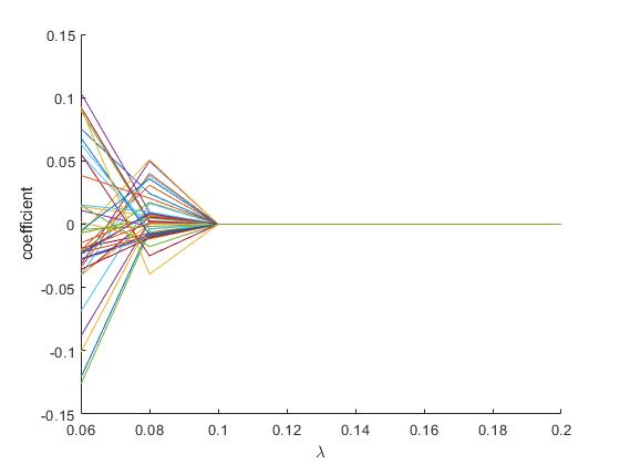
(a) $\theta_{1}$–smoothing

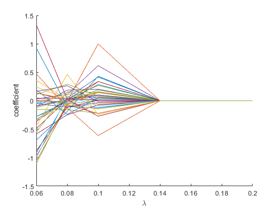
(b) $\theta_{2}$–smoothing.

Figure 1: Problem in dimension $m=20$ and $d=40$.

3.2 Nonlinear ordinary differential equations

A NAVE problem also naturally arises when we deal with a discretization of a nonlinear ordinary differential equation (ODE, for short) involving rough velocity, for example $\dot{\gamma}(t)=\sqrt{|\gamma(t)|}$ as well as an ODE of the form

$$\Phi(X^{(2k)},X^{(2k-1)},\ldots,\dot{X})=|X|$$

In this subsection we provide two examples (one being a stiff ODE) to illustrate the effectiveness of smoothing techniques when using finite difference schemes for ODEs.

Example 3.1.

We consider a stiff ODE with initial value as follows

$$\begin{dcases}\ddot{x}+1001\dot{x}-1000|x|=0,\,t>0\\ x(0)=x_{0}<0,\,\dot{x}(0)=0,\end{dcases}$$ (3.5)

whose exact solution is

$$x_{\text{exact}}(t)=x_{0}\left(-\dfrac{1}{999}e^{-1000t}+\dfrac{1000}{999}e^{-t}\right)\approx x_{0}e^{-t}.$$

Let us consider problem (3.5) in time domain $I=[0,T]$. We use a uniform mesh $\boldsymbol{t}=(t_{i})$, where $t_{i}=ih$ for $i\in\{0,\cdots,N\}$ and $h=T/N$, and the approximation solution will be $\boldsymbol{x}=(x_{i})$ where $x_{i}\approx x(t_{i})$. For the first and the second derivative, we use the 2nd–order approximation

$$\ddot{x}(t_{i})\approx\dfrac{x_{i-2}-2x_{i-1}+x_{i}}{h^{2}}\text{ and }\dot{x}(t_{i})\approx\dfrac{x_{i+1}-x_{i-1}}{2h}.$$

Remarkably, at the final time, the first derivative $\dot{x}(t_{N})$ will be computed via the 2nd–order backward formula $\dot{x}(t_{N})\approx(x_{N-2}-4x_{N-1}+3x_{N})/2h$. Since the initial velocity is zero, using 1st–order backward approximation, we note that $x_{-1}=x_{0}$. The discretization of (3.5) can be written as

$$\dfrac{1}{1000}\boldsymbol{A}\boldsymbol{x}+\dfrac{1001}{1000}\boldsymbol{B}\boldsymbol{x}-|\boldsymbol{x}|=\boldsymbol{b},$$

where $\boldsymbol{A},\boldsymbol{B}\in\mathbb{R}^{N\times N}$ is determined by

$$\boldsymbol{A}=\dfrac{1}{h^{2}}\begin{pmatrix}1&0&0&\cdots&0&0&0\\ -2&1&0&\cdots&0&0&0\\ 1&-2&1&\cdots&0&0&0\\ \cdots&\cdots&\cdots&\cdots&\cdots&\cdots&\cdots\\ 0&0&0&\cdots&1&0&0\\ 0&0&0&\cdots&-2&1&0\\ 0&0&0&\cdots&1&-2&1\end{pmatrix}\text{ and }\,\,\boldsymbol{B}=\dfrac{1}{2h}\begin{pmatrix}0&1&0&\cdots&0&0&0\\ -1&0&1&\cdots&0&0&0\\ 0&-1&0&\cdots&0&0&0\\ \cdots&\cdots&\cdots&\cdots&\cdots&\cdots&\cdots\\ 0&0&0&\cdots&0&1&0\\ 0&0&0&\cdots&-1&0&1\\ 0&0&0&\cdots&1&-4&3\end{pmatrix}$$ (3.6)

Here, vector $\boldsymbol{b}=(b_{i})\in\mathbb{R}^{N}$ is defined by $b_{i}=0$ for $i\geq 2$, $b_{1}=x_{0}(1/(1000h^{2})+1001/(2000h))$ and $b_{2}=-x_{0}/(1000h^{2})$.

In Figure 2.(a), we approximate the solution of equation (3.5) with initial condition $x_{0}=-1$ and time interval $I=[0,5]$. The finite difference scheme was computed with mesh size $h=0.05$ and the error is $9.22e-4$ when applying $\theta_{1}$ and $\theta_{2}$ smoothing funtions. To get convergence rate in Figure 2.(b), we apply difference mesh sizes in the same time interval $I=[0,1]$ and intial condition $x_{0}=-2$.

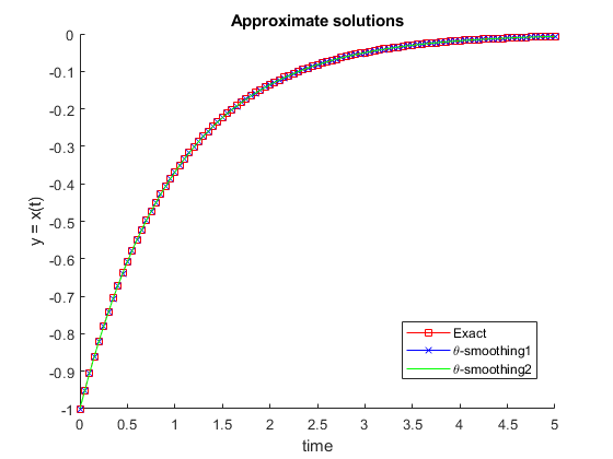
(a) Approximate solutions.

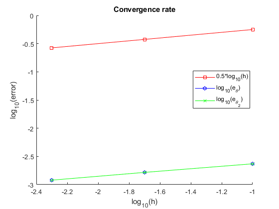
(b) Convergence rate  $O(h^{1/2})$.

Figure 2: Solving equation 3.5

Let us now make some comments on the utility of NAVE for boundary value problems: we consider a boundary value problem related to (3.5)

$$\begin{dcases}\ddot{x}+1001\dot{x}-1000|x|=0,\,t\in(0,T),\\ x(0)=x_{0}<0,\,x(T)=y_{0}\in\mathbb{R}.\end{dcases}$$ (3.7)

In order to illustrate this case, we consider the time interval $I=[0,2]$ and exact solution is determined by $x_{\text{exact}}$. Using similar time mesh as above, the first and second derivatives are approximate as follows

$$\ddot{x}(t_{i})\approx\dfrac{x_{i-1}-2x_{i}+x_{i+1}}{h^{2}}\text{ and }\dot{x}(t_{i})\approx\dfrac{x_{i}-x_{i-1}}{h}.$$

Figure 3 shows the convergence rate for the boundary value problem (3.7). The smoothing technique used in this problem presents a better accuracy compared to the above initial value problem, which seems to be natural because of the stiffness of the problem (3.5). It is noteworthy that Figure 3 also depicts an expected convergence rate since we have used a first order approximation for $\dot{x}$.

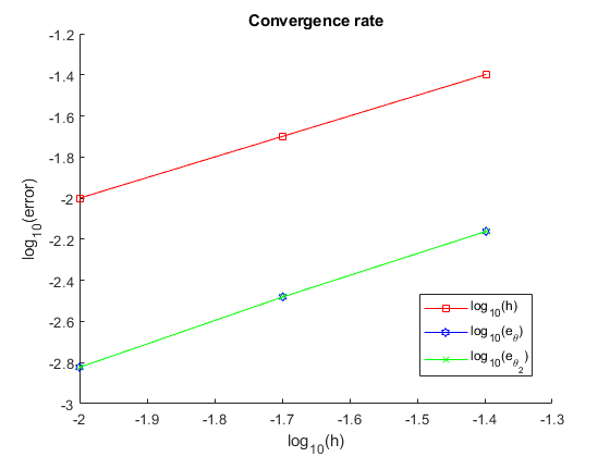
Figure 3: Convergence rate $O(h)$ for a boundary value problem

Example 3.2.

For a continuous function $f:[0,+\infty)\rightarrow\mathbb{R}$, we consider an ODE

$$\begin{dcases}\ddot{x}+\arctan(x)-|x|=f(t),\,t>0,\\ x(0)=x_{0}\in\mathbb{R},\,\dot{x}(0)=0.\end{dcases}$$ (3.8)

Using a similar discretization as in Example 3.1, the unknown variable $\boldsymbol{x}\approx x(\boldsymbol{t})$ solves a NAVE problem as follows

$$\boldsymbol{A}\boldsymbol{x}+\text{arctan}(\boldsymbol{x})-|\boldsymbol{x}|=\boldsymbol{b},$$ (3.9)

where the matrix $\boldsymbol{A}$ is determined as in Example 3.1 and the vector $\boldsymbol{b}\in\mathbb{R}^{N}$ is defined by $b_{i}=f(t_{i})$ for $i\geq 2$ and

$$b_{1}=f(t_{1})+\dfrac{x_{0}}{h^{2}}\text{ and }b_{2}=f(t_{2})-\dfrac{x_{0}}{h^{2}}.$$

To illustrate for this example, we consider problem (3.8) with source term

$$f(t)=\arctan(\cos(\pi t))-|\cos(\pi t)|-\pi^{2}\cos(\pi t),$$

whose exact solution is $x_{exact}(t)=\cos(\pi t)$. Figure 4.(a) shows the approximate solution on the time interval $I=[0,1]$ with mesh size $h=0.0125$. The error between $\theta_{1}$ (resp. $\theta_{2}$) approximation and exact solution is $0.06$ (resp. $0.0725$). Besides, Figure 4.(b) displays convergence rate of the combination of finite difference scheme and the $\theta$–smoothing applying for the associated NAVE problem.

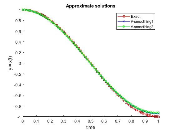
(a) Approximate solutions.

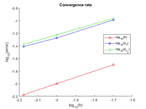
(b) Convergence rate  $O(h)$.

Figure 4: Solving equation 3.8.

3.3 Comparison of methods for NAVE

Instead of smoothing procedure considered in Section 2, one can solve a NCP via other numerical methods. In this subsection we give examples to compare the efficiency of four methods

• Newton–like method with smoothing functions $\theta_{1}$ and $\theta_{2}$;

• approximating by Soft–Max function, in which the main idea is to approximate the complementarity condition via the limit

  $$\max_{i\in\{1,\cdots,d\}}x_{i}=\lim_{r\searrow 0}r\log\left(\sum_{i=1}^{d}e^{x_{i}/r}\right).$$

  which have been widely used in many optimization problems, for example [31, Example 1.30], [28, 19, 20];

• using interior point method, for example, one can find the use of interior point method for complementarity problems in [17, 29, 15, 11].

Now, in the following examples, we solve the system $\tilde{F}(x)-|x|=b$, especially, Example 3.4 and 3.5 can be found in [18, 2].

Example 3.3.

We consider $\tilde{F}(x)=Ax$, where

$$A=\text{tridiag}(-1,4,-1)\in\mathbb{R}^{d\times d},\,x^{*}\in\mathbb{R}^{d},\,b=Ax^{*}-|x^{*}|.$$ (3.10)

Example 3.4.

$\tilde{F}:\mathbb{R}^{3}\rightarrow\mathbb{R}^{3}$ is defined by

$$\tilde{F}(x):=\begin{pmatrix}2x_{1}-2\vskip 3.0pt plus 1.0pt minus 1.0pt\\ 2x_{2}+x_{2}^{3}-x_{3}+3\vskip 3.0pt plus 1.0pt minus 1.0pt\\ x_{2}+2x_{3}+2x_{3}^{3}-3\end{pmatrix}.$$

Example 3.5.

$\tilde{F}:\mathbb{R}^{4}\rightarrow\mathbb{R}^{4}$ is defined by

$$\tilde{F}(x):=\begin{pmatrix}3x_{1}^{2}+x_{1}+2x_{1}x_{2}+2x_{2}^{2}+x_{3}+3x_{4}\vskip 3.0pt plus 1.0pt minus 1.0pt\\ 2x_{1}^{2}+x_{1}+x_{2}^{2}+x_{2}+10x_{3}+2x_{4}\vskip 3.0pt plus 1.0pt minus 1.0pt\\ 3x_{1}^{2}+x_{1}x_{2}+2x_{2}^{2}+3x_{3}+9x_{4}\vskip 3.0pt plus 1.0pt minus 1.0pt\\ x_{1}^{2}+3x_{2}^{2}+2x_{3}+4x_{4}\end{pmatrix}.$$

Table 3.3 compares the four methods: smoothing method with $\theta_{1}$ and $\theta_{2}$, Soft Max (denoted SM) and Interior Point (denoted IP) method on the NAVE problem associated to Example 3.3–3.5. In the first example, the vector $b$ is randomly generated with values in $[-5,5]$ and the problem is considered in dimensions $d=10,50,200$. In Example 3.4 and 3.5, we respectively consider $b_{1}=(-1,-5,10)^{T}$, $b_{2}=(9,-100,10)^{T}$, $b_{3}=(200,0,900)^{T}$, $b^{*}_{1}=(10,10,-12,0)^{T}$, $b^{*}_{2}=(20,-100,-12,1)^{T}$ and $b^{*}_{3}=(200,10,-5,-5)^{T}$. We observe that the smoothing method (especially with $\theta_{2}$–smoothing function) is the most robust among the considered methods. In connection with convergence speed, the interior point method performs much less competitively than the others, while it only reaches $1e-2$ after $N=2000$ iterations. Another point that can be recognized from Table 3.3 is that the Soft Max method could only solve problems with small size, for example for problems in dimension $N=50$ and $N=200$ the singularities appear after less than $100$ iterations.

Table 2: Several methods to solve NAVE

		Error				Iterations
Example	Vector $b$	$\theta_{1}$	$\theta_{2}$	SM	IP	$\theta_{1}$	$\theta_{2}$	SM	IP
3.3	$d=10$	$9.3e-11$	$1.5e-11$	$5.5e-12$	$1.6e-2$	$20$	$13$	$173$	$2000$
	$d=50$	$1.4e-11$	$5.3e-15$	$NaN$	$8.96e-3$	$29$	$41$	$41$	$2000$
	$d=200$	$8.39e-11$	$1.32e-14$	$NaN$	$9.55e-3$	$45$	$76$	$96$	$2000$
3.4	$b_{1}$	$4.7e-11$	$1.7e-11$	$7e-14$	$5.5e-2$	$14$	$9$	$8$	$2000$
	$b_{2}$	$1.7e-11$	$3.6e-11$	$1.8e-12$	$4e-1$	$22$	$16$	$15$	$2000$
	$b_{3}$	$9.3e-11$	$1.4e-13$	$1.4e-13$	$2e+2$	$211$	$205$	$205$	$2000$
3.5	$b^{*}_{1}$	$5.5e-11$	$1.3e-14$	$2e-14$	$7e-2$	$16$	$12$	$12$	$2000$
	$b^{*}_{2}$	$5.5e-11$	$2.2e-14$	$4.7e-14$	$9.1e-1$	$26$	$22$	$16$	$2000$
	$b^{*}_{3}$	$6.1e-11$	$1.4e-10$	$3e+1$	$3.8e-0$	$50$	$43$	$2000$	$2000$

Figure 5(a) and 5(b) display the performance time between different methods for Example 3.3 with the size $n=20$ and Example 3.4, respectively. We did the observation with $50$ samples and the vector $b$ is randomly generated with values in $[-10,10]$. At a first sight, the interior point method appears to be the slowest one in comparison with the other three methods. As shown in Figure 5(a), the $\theta_{1}$–smoothing performs the best choice among all the methods. If we look carefully, in lower dimension as Example 3.4, the Soft Max and $\theta_{2}$–smoothing performs slightly better than $\theta_{1}$–smoothing method.

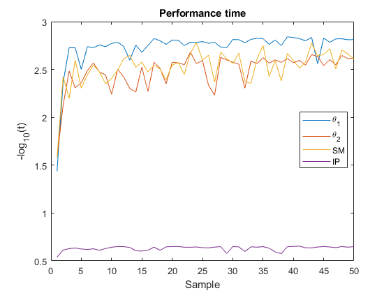
(a) Example 3.1 in dimension $n=20$.

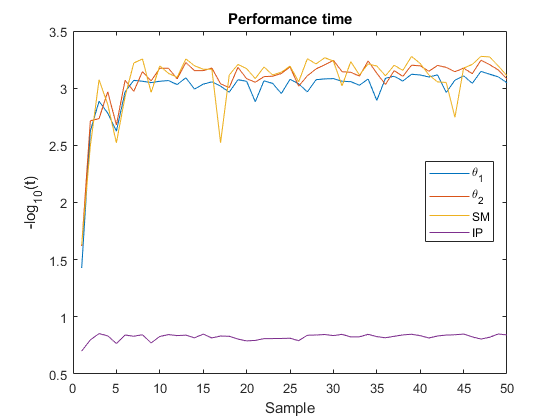
(b) Example 3.2.

Figure 5: Performance time.

Acknowledgement. This work was initiated during a research stay of Aris Daniilidis and Trí Minh Lê to INSA Rennes (February 2023). These authors thank their hosts for hospitality. The first author acknowledges support from the Austrian Science Fund (FWF, P–36344-N).

 

 

Aris Daniilidis, Trí Minh Lê

Institut für Stochastik und Wirtschaftsmathematik, VADOR E105-04
TU Wien, Wiedner Hauptstraße 8, A-1040 Wien
E-mail: {aris.daniilidis, minh.le}@tuwien.ac.at
https://www.arisdaniilidis.at/

Research supported by the grants:
Austrian Science Fund (FWF P-36344N) (Austria)

Mounir Haddou, Olivier Ley

Univ Rennes, INSA, CNRS, IRMAR - UMR 6625, F-35000 Rennes, France
E-mail: {mounir.haddou, olivier.ley}@insa-rennes.fr
http://{haddou, ley}.perso.math.cnrs.fr/

Research supported by the Centre Henri Lebesgue ANR-11-LABX-0020-01.

References

- [1] L. Abdallah, M. Haddou, T. Migot, Solving absolute value equation using complementarity and smoothing functions. J. Comput. Appl. Math. 327 (2018), 196–207.
- [2] J. H. Alcantara, J-S. Chen. A new class of neural networks for NCPs using smooth perturbations of the natural residual function, J. Comput. Appl. Math. 407 (2022), Paper No. 114092, 22 pp.
- [3] J. H. Alcantara, J.-S. Chen, M. K. Tam, Method of alternating projections for the general absolute value equation. J. Fixed Point Theory Appl. 25 (2023), Paper No. 39, 38 pp.
- [4] I. Ben Gharbia J.C. Gilbert, Nonconvergence of the plain Newton-min algorithm for linear complementarity problems with a P-matrix, Mathematical Programming 134 (2012), 349–364.
- [5] J. Y. Bello Cruz, O. P. Ferreira, L. F. Prudente, On the global convergence of the inexact semi-smooth Newton method for absolute value equation, Comput. Optim. Appl. 65 (2016), 93–108.
- [6] M. Coste, An Introduction to o-minimal Geometry, Instituti Editoriali e Poligrafici Internazionali, Pisa (2000).
- [7] D. Dacunto, V. Grandjean, A gradient inequality at infinity for tame functions, Rev. Mat. Complut. 18 (2005), 493–501.
- [8] M. Fiedler, V. Pták, On matrices with nonpositive off-digagonal elements and positive principal minors, Czech. Math. J. 12 (1962), 382–400.
- [9] S.-L. Hu and Z.-H. Huang, A note on absolute value equations, Optim. Lett. 4 (2010), 417–424.
- [10] M. Haddou, P. Maheux, Smoothing methods for nonlinear complementarity problems, J. Optim. Theory Appl. 160 (2014), 711–729.
- [11] M. Haddou, T. Migot, J. Omer, A generalized direction in interior point method for monotone linear complementarity problems, Optim. Lett. 13 (2019), 35–53.
- [12] T. Hastie, Ridge regularization: An essential concept in data science, Technometrics 62 (2020), 426–433.
- [13] T. Hastie, R. Tibshirani, J. Friedman, The elements of statistical learning. Data mining, inference and prediction, Springer (New York, 2001).
- [14] R. W. Hoerl, Ridge regression: A historical context, Technometrics 62 (2020), 420–425.
- [15] A. N. Iusem, An interior point method for the nonlinear complementarity problem, Appl. Numer. Math. 24 (1997), 469–482.
- [16] C. Kanzow, A new approach to continuation methods for complementarity problems with uniform -functions, Oper. Res. Lett. 20 (1997), 85–92.
- [17] M. Kojima, N. Megiddo, T. Noma, A. Yoshise, A unified approach to interior point algorithms for linear complementarity problems, Lecture Notes in Comput. Sci. 538, Springer (Berlin, 1991).
- [18] M. Kojimam S. Shindo, Extension of Newton and quasi-Newton methods to systems of PC1 equations, J. Oper. Res. Soc. Jpn. 29 (1986), 352–374.
- [19] X. Li, An entropy–based aggregate method for minimax optimization, Eng. Opt. 18 (1992), 277–285.
- [20] Y. Li, T. Tan, X. Li, A log-exponential smoothing method for mathematical programs with complementarity constraints, Appl. Math. Comput. 218(2012), 5900–-5909.
- [21] T. L. Loi, Łojasiewicz inequalities in o-minimal structures, Manuscripta Math. 150 (2016), 59–72.
- [22] T. Lotfi and H. Veiseh, A note on unique solvability of the absolute value equation, 2013.
- [23] O. L. Mangasarian, RR. Meyer, Absolute value equations, Linear Algebra Appl. 419 (2006), 359–367.
- [24] O. L. Mangasarian, Linear complementarity as absolute value equation solution, Optim. Lett. 8 (2014), 1529–1534.
- [25] MATLAB R2023A, Natick, Massachusetts: The MathWorks Inc., 2010.
- [26] J.-J. Moré, Global methods for nonlinear complementarity problems, Math. Oper. Res. 21 (1996), 589–614.
- [27] J.-J. Moré , W.C. Rheinboldt, On - and - functions and related classes of - dimensional nonlinear mappings, Linear Algebra Appl. 6 (1973), 45–68.
- [28] Y. Nesterov, Smooth minimization of nonsmooth functions, Math. Program. Ser. A 103 (2005), 127–152.
- [29] F. A. Potra, Y. Ye, Interior-point methods for nonlinear complementarity problems, J. Optim. Theory Appl. 88(1996), 617–642.
- [30] E. H. Osmani, M. Haddou, N. Bensalem, L. Abdallah, A new smoothing method for nonlinear complementarity problems involving -function. Stat. Optim. Inf. Comput. 10 (2022), 1267–1292.
- [31] R. T. Rockafellar, J.-B. R. Wets, Variational analysis, Grundlehren Math. Wiss. 317, Springer (Berlin, 1998).
- [32] O. Prokopyev, On equivalent reformulations for absolute value equations, Comput. Optim. Appl. 44 (2009), 363–372.
- [33] J. Rohn, A theorem of the alternatives for the equation , Linear Mult. Algebra 52 (2004), 421–426.
- [34] J. Rohn, On unique solvability of the absolute value equation, Optim. Lett. 3 (2009), 603–606.
- [35] J. Rohn, V. Hooshyarbakhsh, and R. Farhadsefat, An iterative method for solving absolute value equations and sufficient conditions for unique solvability, Optim. Lett. 8 (2014), 35–44.
- [36] R. Tibshirani, Regression shrinkage and selection via the lasso, J. Roy. Statist. Soc. Ser. B 58 (1996), 267–288.
- [37] S.-L. Wu and C.-X. Li, A note on unique solvability of the absolute value equation, Optim. Lett. 14 (2020), 1957–1960.