Optimization of the Downlink Spectral- and Energy-Efficiency of RIS-aided Multi-user
URLLC MIMO Systems

Abstract

Modern wireless communication systems are expected to provide improved latency and reliability. To meet these expectations, a short packet length is needed, which makes the first-order Shannon rate an inaccurate performance metric for such communication systems. A more accurate approximation of the achievable rates of finite-block-length (FBL) coding regimes is known as the normal approximation (NA). It is therefore of substantial interest to study the optimization of the FBL rate in multi-user multiple-input multiple-output (MIMO) systems, in which each user may transmit and/or receive multiple data streams. Hence, we formulate a general optimization problem for improving the spectral and energy efficiency of multi-user MIMO-aided ultra-reliable low-latency communication (URLLC) systems, which are assisted by reconfigurable intelligent surfaces (RISs). We show that a RIS is capable of substantially improving the performance of multi-user MIMO-aided URLLC systems. Moreover, the benefits of RIS increase as the packet length and/or the tolerable bit error rate are reduced. This reveals that RISs can be even more beneficial in URLLC systems for improving the FBL rates than in conventional systems approaching Shannon rates.

I Introducton

The sixth generation (6G) of wireless communication systems is expected to significantly improve the spectral efficiency (SE), energy efficiency (EE), and reliability of the existing systems, despite of providing a lower latency than 5G [1, 2]. Thus, 6G should employ radical new technologies such as reconfigurable intelligent surface (RIS) to meet these expectations. Moreover, 6G has to support a large variety of applications, which require ultra-reliable and low-latency communications (URLLC) [1, 2]. To attain low latency, realistic finite block length (FBL) codes have to be employed. In this content, the classic Shannon rate is an inaccurate performance metric for URLLC systems. Indeed, the FBL rate is more challenging to optimize than the Shannon rate, especially in multiple-input multiple-output (MIMO) systems, when multi-stream communication is targeted. In fact, to the best of our knowledge, resource allocation has not been designed for multi-user MIMO (MU-MIMO) systems relying on FBL coding in the open literature for the scenario of multiple streams per user. Developing suitable resource allocation schemes is even more challenging in RIS-assisted systems since this requires the joint optimization of the transmit covariance matrices and the channels, which depend on the RIS elements. To close this knowledge gap, we derive a closed-form expression for the rates of users in MU-MIMO systems using realistic FBL coding when multiple streams are allowed. Then, we develop an optimization framework for MU-MIMO RIS-assisted URLLC systems and show that a RIS can substantially improve the SE and EE. Our results show that a RIS can be even more beneficial in MIMO URLLC systems than in systems approaching the classic Shannon rate, since a RIS provides higher gains for short packets and/or for low tolerable bit error rates (BERs).

I-A Literature Review

A main goal of 6G is to drastically enhance the SE and EE, which are even more vital for applications related to FBL coding. To realize this goal, 6G has to employ powerful emerging technologies such as RISs as well as existing MIMO solutions [3, 4]. A RIS was shown to be able to substantially enhance the EE and SE [5, 6, 7, 8, 9, 10], when studying different performance metrics such as the sum rate, minimum rate, total power consumption required for achieving a specific quality of service (QoS), minimum signal-to-interference-plus-noise ratio (SINR), global EE (GEE), and interference leakage. For instance in [5], the authors proposed algorithms for increasing the GEE and sum rate of a multiple-input single-output (MISO) broadcast channel (BC). In [6], it was shown that a RIS reduces the power consumption of the single-cell MISO BC when a minimum SINR per user has to be ensured. Moreover, the authors of [7] showed that a RIS is capable of increasing the minimum SINR of a single-cell MISO BC for a given power budget. The benefit of RIS in terms of both the minimum rate and the minimum EE was studied in [8] for a multi-cell MISO BC employing non-orthogonal multiple access (NOMA). Furthermore, the authors of [9] studied the interference leakage in a MIMO-aided $K$-user interference channel assisted by RIS, showing that an appropriately designed RIS mitigates the total interference power of the system.

The performance of RIS relying on the Shannon capacity achieving codes has been studied in [5, 6, 7, 8, 9], but naturally, a RIS can also be beneficial in multi-user systems using FBL coding, as shown in [11, 12, 13, 14, 15, 16]. For instance, in [11], resource allocation schemes were developed for MISO URLLC systems, assisted by simultaneously transmit and reflect (STAR-) RIS, and it was shown that a RIS (either STAR or purely reflective) substantially improves the SE and EE of URLLC systems. In [12], it was demonstrated that RIS and rate splitting can be mutually beneficial tools of enhancing the EE and SE performance of interference-limited URLLC systems. In [14], the advantage of employing a RIS and NOMA in a two-user single-input single-output (SISO) URLLC BC was shown.

All the aforementioned papers [11, 12, 13, 14, 15, 16] studied multi-user RIS-assisted URLLC systems, but only supported single-stream data transmission per user. However, RIS can also improve the system performance when parallel frequency-domain channels are employed along with FBL coding [17]. Nevertheless, resource allocation has not been designed for multi-user MIMO URLLC systems supporting multiple streams per user in the open literature. This is particularly challenging for RIS-assisted systems. Indeed, only a few treatises exist in multiple-stream data transmission in MIMO systems, which mainly studied a single-user scenario without considering RISs [18, 19, 20]. Thus, multi-user MIMO systems both with and without RISs require further investigations. MIMO systems support multiple-stream data transmissions per user, which exploit the spectrum efficiently and improve the EE at a specific QoS. Below, we briefly describe the challenges of optimizing the FBL rates when multiple-stream data transmission is supported.

In the FBL regime, the achievable rate depends not only on the Shannon rate, $C$, but also on the channel’s dispersion, $V$, the packet length, $n_{t}$, and the tolerable bit error rate $\epsilon$. An accurate approximation for the achievable rate of FBL coding in parallel channels is the normal approximation (NA), which is given by [24, Theorem 78]

$$r=\sum_{i=1}^{I}C_{i}-Q^{-1}(\epsilon)\sqrt{\frac{\sum_{i=1}^{I}V_{i}}{n_{t}}},$$ (1)

where $Q^{-1}$ is the inverse of the well-known $Q$ function of Gaussian distributions, $I$ is the number of parallel channels, $C_{i}$ and $V_{i}$ are, respectively, the Shannon rate and the channel dispersion of the $i$-th parallel channel. Note that the channel dispersion and Shannon rate of parallel channels are, respectively, a summation of the channel dispersions and Shannon rates of all individual channels, i.e., $C=\sum_{i=1}^{I}C_{i}$ and $\sum_{i=1}^{I}V_{i}$. The Shannon rate of MIMO systems can also be represented in a closed-form matrix format, and there are already existing contributions on optimizing the Shannon rates in MIMO RIS-assisted systems [25, 26]. However, the achievable channel dispersion term for Gaussian signals has a fractional structure, which is more challenging to optimize, and its closed-form matrix format has not been derived in the related works. Hence, resource allocation for parallel channels relying on FBL coding can be much more complicated than for single-stream channels. Moreover, the channel’s dispersion term makes it impossible to reuse the existing solutions for MIMO RIS-assisted systems, when FBL coding is employed. In the next subsection, we provide a critical review of the existing works on RIS-assisted URLLC systems and discuss the open topics that merit further investigations.

TABLE I: Overview of most closely related works on RIS-assisted URLLC systems.

	Multi-user	Channel dispersion in [27]	EE	MIMO	Multiple streams	STAR-RIS
This paper	$\surd$	$\surd$	$\surd$	$\surd$	$\surd$	$\surd$
[12]	$\surd$	$\surd$	$\surd$	-	-	-
[28]	$\surd$	$\surd$	-	-	-	-
[13, 14, 15, 16, 17, 29]	$\surd$	-	-	-	-	-
[30, 31]	-	-	-	-	-	-

I-B Motivation

The most closely related treatises on RIS-assisted URLLC system designs are compared in Table I, based on the system model, network scenario, performance metrics, and the channel dispersion encountered in multi-user systems. As shown in the table, most of the studies on FBL transmission in RIS-assisted systems have focused on SISO/MISO systems, when only a single-stream data transmission per user is allowed. Additionally, there is a limited number of contributions on EE in RIS-assisted URLLC systems and EE metrics have not been studied in multi-user MIMO systems using FBL coding. Note that in URLLC systems, the EE can be even more vital, since in some applications, it might be impossible to replace the battery of users/nodes, and consequently, the network must be as energy efficient as possible.

Moreover, there is no work on multi-user MIMO systems with FBL considering the achievable channel dispersion term in [27], even for systems without RIS. It should be emphasized that Gaussian signaling cannot achieve the optimal channel dispersion in the presence of interference in multi-user systems. Hence, when employing Gaussian signaling, it is more accurate to consider the suboptimal channel dispersion term in [27] instead of the optimal one since the channel dispersion in [27] can be attained through Gaussian signals in the presence of both interference and white additive Gaussian noise in multi-user systems.

To sum up, resource allocation schemes should be developed for multi-user RIS-assisted URLLC MIMO systems with more emphasis on EE and by allowing multiple-data-stream transmissions per user and considering the achievable channel dispersion term for Gaussian signals. Thus, a general optimization framework for multi-user RIS-assisted MIMO systems with FBL coding can facilitate future studies in this field.

I-C Contribution

We propose a general optimization framework for maximizing the SE and EE of multi-user MIMO RIS-aided URLLC systems. To the best of our knowledge, this is the first paper on the resource allocation of MU-MIMO RIS-aided URLLC systems supporting multiple stream per users. To develop a general framework, we first formulate a closed-form expression for the channel dispersion of MIMO systems in the presence of interference, based on both the optimal channel dispersion as well as on the channel dispersion term in [27]. Then, we propose specific schemes for optimizing the FBL rate expressions by employing majorization minimization (MM), alternating optimization (AO), and fractional programming (FP) tools such as Dinkelbach-based algorithms. As indicated in Section I-A, due to the channel dispersion term, which has a fractional structure, the FBL rates are much more challenging to optimize than the classic Shannon rates. Moreover, it is impossible to adapt the established works on MIMO RIS-assisted systems with Shannon rates to the systems with FBL coding, and to evaluate how the reliability and latency constraints influence the effectiveness of RISs. Thus, the main novelty of this treatise is the derivation of closed-form expressions for the channel dispersion, followed by the development of algorithms to optimize over the FBL rates, including the dispersion term.

To elaborate, our optimization framework is flexible and can be utilized in any MU-MIMO URLLC system aided by RISs. Furthermore, the framework may be used for solving a broad spectrum of optimization problems for which the objective function and/or constraints are linear functions of the rates and/or EE of users. The convergence of our framework is ensured towards a stationary point for the general optimization problem, when the feasibility set for the RIS elements conforms to a convex set. We consider a multi-cell MIMO BC as an example of the networks that our framework can be applied to. Furthermore, we consider both the EE and SE metrics for investigating the performance of RIS in MU-MIMO URLLC systems. For the SE metric, we consider the sum rate and the minimum rate of the users, which are among the most common performance metrics for SE. Moreover, we evaluate the EE by optimizing the GEE and the minimum EE of users. Note that the sum rate and global EE are pivotal overall system performance metrics. By contrast, the minimum rate and the EE of specific users consider the individual performance of the users and can provide reasonable rate/EE-fairness among the users since typically all the users are allocated similar rate/EE when the minimum rate/EE is maximized. Thus, considering all these metrics can provide a complete picture of the performance of MU-MIMO URLLC systems aided by RISs. Moreover, we make realistic assumptions regarding the channel models and the feasible sets of the RIS coefficients for appropriately examining the RIS performance.

In addition to passive and reflective RISs, we also consider simultaneously transmitting and reflecting (STAR) RIS, which provides a full $360^{\circ}$ coverage. Moreover, we show that RISs can significantly enhance the EE and SE of a multi-user MIMO URLLC BC. Notably, the advantages of RISs escalate with shorter packet lengths and/or more stringent reliability constraints. This implies that the benefits of RIS can be higher in MU-MIMO URLLC systems. However, it should be noted that the performance of the system may become degraded, if the RIS elements are inaccurately optimized.

I-D Organization and Notations

The structure of the paper is outlined in the following. Section II describes our network scenario, RIS model, and signal model as well as the rate and EE expressions. Moreover, in Section II, we formulate the optimization problem considered. Section III presents the optimization framework proposed. Section IV presents our numerical results. Finally, Section V concludes the paper.

The trace and determinant of the matrix ${\bf X}$ are, respectively, denoted as $\text{Tr}({\bf X})$ and $|{\bf X}|$. We represent the conjugate of complex variable/vector/matrix $x/{\bf x}/{\bf X}$ as $x^{*}/{\bf x}^{*}/{\bf X}^{*}$. The mathematical expectation is denoted as $\mathbb{E}\{\cdot\}$. The identity matrix is represented as ${\bf I}$. Moreover, $\mathcal{O}[\cdot]$ is the big-O notation for representing the computational complexity of algorithms.

II System model

Our proposed framework can be applied to any RIS-assisted MU-MIMO URLLC system that treats interference as noise at the receivers. As an example of such MU-MIMO systems, we consider a multicell MIMO RIS-assisted downlink (DL) BC comprising $L$ BSs, as shown in Fig. 1. We assume that each BS has $N_{BS}$ the DL transmission antennas (TAs) and serves $K$ users having $N_{u}$ receive antennas (RAs) each. Furthermore, we assume that there are $M$ reflective passive RISs to assist the BSs, and each RIS has $N_{RIS}$ elements. Additionally, we assume having perfect, instantaneous, and global CSI. For notational simplicity, we consider a symmetric scenario in which all the BSs/users/RISs employ similar devices without loss of generality. However, the framework can be applied to asymmetric systems having an arbitrary number of antennas at the transmit and receive sides, and different number of users per cell.

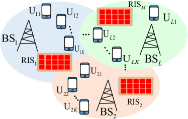
Figure 1: A multicell BC assisted by RISs.

II-A RIS Model

We employ the RIS model of [32] for the MIMO multicell BC. The channel matrix between BS $i$ and the $k$-th user associated to BS $l$, denoted as U_lk, as a function of the RIS matrices is given by

$$\mathbf{H}_{lk,i}\!\left(\{\bf{\Psi}\}\right)\!\!=\!\!\underbrace{\sum_{m=1}^{M}\mathbf{G}_{lk,m}{\bf\Psi}_{m}\mathbf{G}_{m,i}}_{\text{Link through RIS}}+\!\!\!\underbrace{\mathbf{F}_{lk,i}}_{\text{Direct link}}\!\!\!\!\in\mathbb{C}^{N_{u}\times N_{BS}}\!\!,$$ (2)

where $\mathbf{F}_{lk,i}\in\mathbb{C}^{N_{u}\times N_{BS}}$ is the channel matrix between the $i$-th BS and U_lk, $\mathbf{G}_{lk,m}\in\mathbb{C}^{N_{u}\times N_{RIS}}$ is the channel matrix between the $m$-th RIS and U_lk, and $\mathbf{G}_{m,i}\in\mathbb{C}^{N_{RIS}\times N_{BS}}$ is the channel matrix between the $i$-th BS and the $m$-th RIS. Additionally, $\{{\bf\Psi}\}=\{{\bf\Psi}_{m}\}_{m=1}^{M}$ denotes the set of all coefficients of RISs, where ${\bf\Psi}_{m}\in\mathbb{C}^{N_{RIS}\times N_{RIS}}$ is a diagonal matrix, containing the vector of reflecting coefficients of the $m$-th RIS

$${\bf\Psi}_{m}=\text{diag}\left(\psi_{m_{1}},\psi_{m_{2}},\cdots,\psi_{m_{N_{RIS}}}\right).$$

Assuming having passive RISs, the absolute value of the RIS coefficients cannot be greater than 1, which results in the following set for the feasible RIS coefficients [3, Eq. (11)]

$$\mathcal{T}_{U}=\left\{\psi_{m_{n}}:|\psi_{m_{n}}|^{2}\leq 1\,\,\,\forall m,n\right\}.$$ (3)

In this feasibility set, the amplitude and phase of each RIS element are assumed to be independent optimization variables, which might not be realistic. Another common assumption is that the RIS coefficients have to adhere to the unit modulus constraint [4, 3, 6, 7, 33, 32, 34], which leads to the set

$$\mathcal{T}_{I}=\left\{\psi_{m_{n}}:|\psi_{m_{n}}|=1\,\,\,\forall m,n\right\}.$$ (4)

In this feasibility set, the amplitude of each RIS coefficient is assumed to be equal to 1, while the phases can be optimized. As $\mathcal{T}_{I}\subset\mathcal{T}_{U}$, it can be expected that the algorithms for $\mathcal{T}_{U}$ outperform the algorithms for $\mathcal{T}_{I}$.

Again, another technology for RIS that we consider is STAR-RIS, which provides an omni-directional $360^{\circ}$ full-place coverage. In STAR-RIS, each component can operate in both reflection and transmission mode [35, 36]. Thus, there are two complex-valued optimization parameters per element, when STAR-RIS is employed. We denote the reflection/transmission coefficient for the $n$-th element of the $m$-th RIS as $\psi_{m_{n}}^{r}/\psi_{m_{n}}^{t}$. Based on the position of the user with respect to STAR-RIS, the STAR-RIS can optimize the channel of the user only through the reflection or transmission coefficients. Therefore, the channel between BS $i$ and U_lk is

$$\mathbf{H}_{lk,i}\left(\{\bf{\Psi}\}\right)={\sum_{m=1}^{M}\mathbf{G}_{lk,m}{\bf\Psi}_{m}^{t/r}\mathbf{G}_{m,i}}+{\mathbf{F}_{lk,i}},$$ (5)

where we have ${\bf\Psi}_{m}^{r}=\text{diag}\left(\psi_{m_{1}}^{r},\psi_{m_{2}}^{r},\cdots,\psi_{m_{N_{RIS}}^{r}}\right)$ and ${\bf\Psi}_{m}^{t}=\text{diag}\left(\psi_{m_{1}}^{t},\psi_{m_{2}}^{t},\cdots,\psi_{m_{N_{RIS}}^{t}}\right)$. Assuming operating in a passive mode, the absolute values of the reflection and transmission coefficients have to satisfy

$$|\psi_{m_{n}}^{r}|^{2}+|\psi_{m_{n}}^{t}|^{2}\leq 1,\hskip 28.45274pt\forall mn,$$ (6)

which yields the set

$$\mathcal{T}_{SU}=\left\{\psi_{m_{n}}^{r},\psi_{m_{n}}^{t}:|\psi_{m_{n}}^{r}|^{2}+|\psi_{m_{n}}^{t}|^{2}\leq 1\,\,\,\forall m,n\right\}.$$ (7)

Assuming operating in the passive mode with equal input and output powers, we have

$$|\psi_{m_{n}}^{r}|^{2}+|\psi_{m_{n}}^{t}|^{2}=1,\hskip 28.45274pt\forall m,n,$$ (8)

which results in

$$\mathcal{T}_{SI}=\left\{\psi_{m_{n}}^{r},\psi_{m_{n}}^{t}:|\psi_{m_{n}}^{r}|^{2}+|\psi_{m_{n}}^{t}|^{2}=1\,\,\,\forall m,n\right\}.$$ (9)

There are three different STAR-RIS schemes, including the energy splitting (ES), mode switching (MS) and time switching (TS) schemes [37, 36]. Since the main focus of this work is on evaluating the impact of employing multiple streams per user regimes, we consider only the MS scheme. Note that the MS scheme has a lower implementation complexity than the ES scheme, but its performance may be comparable to that of the ES scheme as shown in, e.g., [38, 39, 40]. The framework proposed in this treatise can be extended to include the ES and TS schemes by following an approach similar to [39, 40]. Note that there are other RIS technologies and/or more practical feasibility sets for STAR/reflective RIS as mentioned in [3, 41], which should be considered in future studies.

It is worth emphasizing that the channel matrices are assumed to be linear/affine functions of the RIS elements. To simplify the notations/equations, we remove this dependency and subsequently denote the channels as $\mathbf{H}_{lk,i}$ for all $l,k,i$, hereafter. Additionally, we denote the set of the feasible RIS elements as $\mathcal{T}$, unless we refer to a specific set.

II-B Signal Model

We assume that BS $l$ broadcasts the signal

$${\bf x}_{l}=\sum_{k=1}^{K}{\bf x}_{lk}\in\mathbb{C}^{N_{BS}\times 1},$$ (10)

where ${\bf x}_{lk}$ is the signal intended for user U_lk, which is a zero-mean complex Gaussian random vector with covariance ${\bf P}_{lk}=\mathbb{E}\{{\bf x}_{lk}{\bf x}_{lk}^{H}\}$, where $\mathbb{E}\{{\bf x}\}$ is the mathematical expectation of ${\bf x}$. We assume that the zero-mean signals ${\bf x}_{lk}$ are independent from each other, i.e., $\mathbb{E}\{{\bf x}_{lk}{\bf x}_{ij}^{H}\}={\bf 0}$ for $i\neq l$ and/or $j\neq k$. Additionally, we denote the covariance matrix of ${\bf x}_{l}$ by ${\bf P}_{l}=\mathbb{E}\{{\bf x}_{l}{\bf x}_{l}^{H}\}$. Since the signal ${\bf x}_{lk}$ are zero-mean and independent random vectors, we have $\mathbf{P}_{l}=\sum_{k}\mathbf{P}_{lk}$. The set containing all the feasible transmit covariance matrices is denoted as $\mathcal{P}$ and it is given by

$$\mathcal{P}=\left\{\mathbf{P}_{lk}:\text{Tr}\left(\mathbf{P}_{l}\right)\leq p_{l},\mathbf{P}_{lk}\succcurlyeq\mathbf{0},\,\,\forall l,k\right\},$$ (11)

where $p_{l}$ is the power budget of the $l$-th BS.

The received signal at U_lk is given by

$${\bf y}_{lk} =\sum_{i}{\bf H}_{lk,i}{\bf x}_{i}+{\bf n}_{lk},$$

$$=\!\!\underbrace{{\bf H}_{lk,l}{\bf x}_{lk}}_{\text{Desired Signal}}\!+\!\!\underbrace{\sum_{j\neq k}{\bf H}_{lk,l}{\bf x}_{lj}}_{\text{Intra-cell Interference}}\!+\!\underbrace{\sum_{i\neq l}{\bf H}_{lk,i}{\bf x}_{i}}_{\text{Intercell Interference}}\!+\!\underbrace{{\bf n}_{lk}}_{\text{Noise}},$$

where ${\bf n}_{lk}$ is the zero-mean additive white Gaussian noise at U_lk with covariance matrix $\sigma^{2}{\bf I}$, where ${\bf I}$ denotes the identity matrix.

II-C Channel Dispersion, Rate and EE Expressions

A MIMO channel can be modeled as a set of parallel AWGN channels, and [24, Theorem 78] can be employed to obtain the achievable rate of MIMO channels associated with FBL coding. Note that [24, Theorem 78] is based on the optimal power allocation for a point-to-point MIMO communication link; however, the FBL rate expressions can be formulated for any arbitrary power allocation as shown in [24, Section 4.5.4]. In the following lemma, we calculate the achievable FBL rate of users, when the interference is treated as noise for decoding the corresponding signal at the receivers.

Lemma 1 (​[24]).

The second-order rate of user U_lk for FBL coding along with the normal approximation (NA) is given by

$$r_{lk}=\underbrace{\log\left|{\bf I}+{\bf D}^{-1}_{lk}{\bf S}_{lk}\right|}_{\text{\small Shannon Rate}}-Q^{-1}(\epsilon)\sqrt{\frac{V_{lk}}{n_{t}}},$$ (12)

where $n_{t}$ is the packet length, ${\bf S}_{lk}={\bf H}_{lk,l}{\bf P}_{lk}{\bf H}_{lk,l}^{H}$ is the covariance matrix of the desired signal at the user U_lk, while ${\bf D}_{lk}$ is the covariance matrix of the interfering signals plus noise, given by

$${\bf D}_{lk}=\sigma^{2}{\bf I}+\sum_{i=1,i\neq l}^{L}{\bf H}_{lk,i}{\bf P}_{i}{\bf H}_{lk,i}^{H}+\sum_{j=1,j\neq k}^{K}{\bf H}_{lk,l}{\bf P}_{lj}{\bf H}_{lk,l}^{H}.$$ (13)

Here, the first-order Shannon rate can also be written as

$$C_{lk}={\log\left|{\bf I}+{\bf D}^{-1}_{lk}{\bf S}_{lk}\right|}=\log\left|{\bf I}+{\bf\Lambda}_{lk}\right|=\sum_{i=1}^{I}\log\left(1+\lambda_{lki}\right),$$ (14)

where ${\bf\Lambda}_{lk}=\text{diag}\left(\lambda_{lk1},\lambda_{lk2},\cdots,\lambda_{lkI}\right)$ is a diagonal matrix, containing the non-zero eigenvalues of the positive semidefinite (PSD) matrix ${\bf D}^{-1}_{lk}{\bf S}_{lk}$, and $I\leq\min(N_{BS},N_{u})$ is equal to the rank of ${\bf H}_{lk,l}{\bf P}_{lk}{\bf H}_{lk,l}^{H}$, which also represents the number of parallel channels. The parameter $\lambda_{lki}$ is actually the signal-to-interference-plus-noise ratio (SINR) at the $i$-th parallel channel of user U_lk. Finally, $V_{lk}=\sum_{i=1}^{I}V_{lki}$ is the channel dispersion of U_lk, where $V_{lki}$ is the channel dispersion of the $i$-th parallel channel of user U_lk.

The optimal channel dispersion of the $i$-th parallel channel is given by [27]

$$V_{lki}=1-\frac{1}{(1+\lambda_{lki})^{2}},$$ (15)

where is $\lambda_{lki}$ is given in Lemma 1. Unfortunately, the optimal channel dispersion attains the minimum value of $V_{lki}$ for all $l$, $k$, and $i$, but Gaussian signals cannot achieve it in the presence of interference. In [27], a coding scheme was proposed for independent, identically distributed (iid) Gaussian signals in interference channels, which has the following channel dispersion

$$V_{lki}=2\left(1-\frac{1}{1+\lambda_{lki}}\right).$$ (16)

In the following lemma, we present closed-form matrix expressions for the optimal channel dispersion and the achievable channel dispersion in (12).

Lemma 2.

The optimal channel dispersion can be written as

$$V_{lk}=\text{\em Tr}\left({\bf I}-({\bf I}+{\bf D}^{-1}_{lk}{\bf S}_{lk})^{-2}\right).$$ (17)

Additionally, the achievable channel dispersion for the scheme proposed in [27] can be written in the following matrix format

$$V_{lk} =2\text{\em Tr}\left({\bf I}-({\bf I}+{\bf D}^{-1}_{lk}{\bf S}_{lk})^{-1}\right)$$ (18)

$$=2\text{\em Tr}\left({\bf I}-{\bf D}_{lk}({\bf D}_{lk}+{\bf S}_{lk})^{-1}\right)$$ (19)

$$=2\text{\em Tr}\left({\bf S}_{lk}({\bf D}_{lk}+{\bf S}_{lk})^{-1}\right).$$ (20)

Proof.

It is widely exploited that the trace of a positive semi-definite matrix is equal to the summation of its eigenvalues. It can be readily verified that the non-zero eigenvalues of $({\bf I}+{\bf D}^{-1}_{lk}{\bf S}_{lk})^{-2}$ are equal to $\left(1+\lambda_{lki}\right)^{-2}$, $i\in\{1,2,\cdots,I\}$, which proves the equality in (17). Note that if ${\bf X}$ is a positive semi-definite matrix with non-zero eigenvalues $\lambda_{i}$, then its pseudo-inverse, denoted as ${\bf X}^{-1}$, is also a positive semi-definite matrix, and its non-zero eigenvalues are $\lambda_{i}^{-1}$.

Similarly, it can be readily verified that the eigenvalues of $({\bf I}+{\bf D}^{-1}_{lk}{\bf S}_{lk})^{-1}$ are equal to $\left(1+\lambda_{lki}\right)^{-1}$, $i\in\{1,2,\cdots,I\}$, which yields (18). Employing a simple matrix factorization, it can be easily verified that (18), (19), and (20) are equivalent. ∎

The EE of U_lk is defined as [42]

$$e_{lk}=\frac{r_{lk}}{p_{c}+\eta\text{Tr}\left(\mathbf{P}_{lk}\right)},$$ (21)

where $\eta^{-1}$ is the power efficiency of the transmit devices at the BSs, $p_{c}$ is the constant power consumption of the system (including the devices of the BSs, RISs and U_lk) to transmit data to a user, which is given by [25, Eq. (27)], and $r_{lk}$ is given by Lemma 1. Note that to compute $p_{c}$, the constant power of the devices of the BSs and RISs is normalized by the number of users served. Moreover, the global EE (GEE) of the network is defined as [42]

$$g=\frac{\sum_{lk}r_{lk}}{LKp_{c}+\eta\sum_{l}\text{Tr}\left(\mathbf{P}_{l}\right)},$$ (22)

which quantifies how energy efficient the network is.

II-D Problem Statement

We consider a general optimization problem for URLLC systems formulated as follows

$$\underset{\{\mathbf{P}\}\in\mathcal{P},\{\bf{\Psi}\}\in\mathcal{T}}{\max}\,\,\, f_{0}\!\left(\left\{\mathbf{P}\right\}\!,\!\{\bf{\Psi}\}\right)\!\!\!\!$$ (23a)

s.t. $$f_{i}\left(\left\{\mathbf{P}\right\}\!,\!\{\bf{\Psi}\}\right)\geq 0,\,\forall i,$$ (23b)

$$r_{lk}\geq r^{th},\,\,\,\,\forall l,k,$$ (23c)

where constraint (23c) can be interpreted as a latency constraint for each user, as discussed in [11, Sec. II.D]. Moreover, functions $f_{i}$, $\forall i$ are linear functions of the rates/EEs and/or transmit/receive powers. The general problem in (23) can include an extensive range of practical optimization scenarios including the maximization of the minimum weighted rate, sum rate, global EE and minimum EE. We refer the reader to [43, Sec. II.B] for more discussions on the format of the functions $f_{i}$s as well as of the family of optimization problems that can be formulated as (23).

III Proposed optimization framework

In this section, we propose iterative schemes for solving (23) by leveraging AO, MM-based, and FP algorithms. Specifically, we first fix the RIS coefficients to $\{{\bf\Psi}^{(t-1)}\}$ and update the transmit covariance matrices as $\{{\bf P}^{(t)}\}$ by solving (23). We then alternate and update the RIS coefficients, while $\{{\bf P}\}$ is fixed to $\{{\bf P}^{(t)}\}$. We iterate this procedure until convergence is reached. Unfortunately, the optimization problems are non-convex and complicated even when the RIS elements (or covariance matrices) are fixed. Thus, we propose a suboptimal scheme based on MM to solve the corresponding problems. Below, we present our solutions for updating the transmit covariance matrices and RIS elements in separate subsections.

III-A Updating Transmit Covariance Matrices

To update $\{{\bf P}\}$, we introduce a new set of variables $\{{\bf Q}\}=\{{\bf Q}_{lk}\}_{\forall lk}$, where ${\bf Q}_{lk}$ is a positive semi-definite matrix and ${\bf P}_{lk}={\bf Q}_{lk}{\bf Q}_{lk}^{H}$. Equivalently, we can compute ${\bf Q}_{lk}$ as ${\bf P}_{lk}^{1/2}$. To attain a suboptimal solution for (23), we leverage an MM-based technique. More specifically, we first obtain suitable concave surrogate functions for the rates. Then, we update ${\bf P}_{lk}^{(t)}={\bf Q}_{lk}^{(t)}{\bf Q}_{lk}^{(t)^{H}}$, $\forall l,k$, by solving the corresponding surrogate optimization problems. To derive concave lower bounds for the FBL rates, we utilize the bounds in the following lemmas.

Lemma 3.

Consider the arbitrary matrices ${\bf\Lambda}$, $\bar{\bf\Lambda}$ and positive semi-definite matrices ${\bf\Upsilon}$, $\bar{\bf\Upsilon}$. Then, the following inequality holds for all feasible ${\bf\Lambda}$, $\bar{\bf\Lambda}$, ${\bf\Upsilon}$, and $\bar{\bf\Upsilon}$:

$$f\left({\bf\Lambda},{\bf\Upsilon}\right)=\text{\em Tr}\left({\bf\Upsilon}^{-1}{\bf\Lambda}{\bf\Lambda}^{H}\right)\geq 2\mathfrak{R}\left\{\text{\em Tr}\left(\bar{\bf\Upsilon}^{-1}\bar{\bf\Lambda}{\bf\Lambda}^{H}\right)\right\}\\ -\text{\em Tr}\left(\bar{\bf\Upsilon}^{-1}\bar{\bf\Lambda}\bar{\bf\Lambda}^{H}\bar{\bf\Upsilon}^{-1}{\bf\Upsilon}\right),$$ (24)

where $\mathfrak{R}\{x\}$ returns the real value of $x$.

Proof.

Function $f\left({\bf\Lambda},{\bf\Upsilon}\right)$ is jointly convex in ${\bf\Lambda}$ and ${\bf\Upsilon}$ [44]. Thus, we can employ the first-order Taylor expansion to obtain an affine lower-bound for $f(\cdot)$ as follows

$$f\left({\bf\Lambda},{\bf\Upsilon}\right)\geq f\left(\bar{\bf\Lambda},\bar{\bf\Upsilon}\right)+2\mathfrak{R}\left\{\frac{\partial f\left({\bf\Lambda},{\bf\Upsilon}\right)}{\partial{\bf\Lambda}}|_{\bar{\bf\Lambda},\bar{\bf\Upsilon}}\left({\bf\Lambda}-\bar{\bf\Lambda}\right)\right.\\ +\left.\frac{\partial f\left({\bf\Lambda},{\bf\Upsilon}\right)}{\partial{\bf\Upsilon}}|_{\bar{\bf\Lambda},\bar{\bf\Upsilon}}\left({\bf\Upsilon}-\bar{\bf\Upsilon}\right)\right\},$$ (25)

where $\bar{\bf\Lambda}$ and $\bar{\bf\Upsilon}$ are any arbitrary feasible points, and $\frac{\partial f\left({\bf\Lambda},{\bf\Upsilon}\right)}{\partial{\bf\Lambda}}|_{\bar{\bf\Lambda},\bar{\bf\Upsilon}}$ (or $\frac{\partial f\left({\bf\Lambda},{\bf\Upsilon}\right)}{\partial{\bf\Upsilon}}|_{\bar{\bf\Lambda},\bar{\bf\Upsilon}}$) is the derivative of $f(\cdot)$ with respect to ${\bf\Lambda}$ (or ${\bf\Upsilon}$) at $\bar{\bf\Lambda}$ and $\bar{\bf\Upsilon}$. Replacing the corresponding derivatives in (25) and simplifying the equation results in (24). ∎

Lemma 4 (​[25]).

Consider the arbitrary matrices ${\bf\Lambda}$ and $\bar{{\bf\Lambda}}$, and positive definite matrices ${\bf\Upsilon}$ and $\bar{{\bf\Upsilon}}$. Then, we have:

$$\ln\left|\mathbf{I}+{\bf\Upsilon}^{-1}{\bf\Lambda}{\bf\Lambda}^{H}\right|\geq\ln\left|\mathbf{I}+{\bf\Upsilon}^{-1}\bar{{\bf\Lambda}}\bar{{\bf\Lambda}}^{H}\right|\\ -\text{{\em Tr}}\left(\bar{{\bf\Upsilon}}^{-1}\bar{{\bf\Lambda}}\bar{{\bf\Lambda}}^{H}\right)+2\mathfrak{R}\left\{\text{{\em Tr}}\left(\bar{{\bf\Upsilon}}^{-1}\bar{{\bf\Lambda}}{\bf\Lambda}^{H}\right)\right\}\\ -\text{{\em Tr}}\left((\bar{{\bf\Upsilon}}^{-1}-(\bar{{\bf\Lambda}}\bar{{\bf\Lambda}}^{H}+\bar{{\bf\Upsilon}})^{-1})^{H}({\bf\Lambda}{\bf\Lambda}^{H}+{\bf\Upsilon})\right).$$ (26)

Upon employing the concave lower bounds in Lemma 3 and Lemma 4, we can obtain a concave lower bound for the FBL rates with the NA approximation as presented in the following lemma.

Lemma 5.

A concave lower bound for $r_{lk}$ is given by

$$r_{lk}\geq\tilde{r}_{lk}=a_{lk}+2\sum_{ij}\mathfrak{R}\left\{\text{{\em Tr}}\left({\bf A}_{lk,ij}\mathbf{Q}_{ij}^{H}\bar{\mathbf{H}}_{lk,i}^{H}\right)\right\}\\ -\text{{\em Tr}}\left({\bf B}_{lk}(\bar{\bf H}_{lk,l}\mathbf{Q}_{lk}\mathbf{Q}_{lk}^{H}\bar{\bf H}_{lk,l}^{H}+\mathbf{D}_{lk})\right)$$ (27)

where

$$a_{lk} \!=\!\ln\left|\!{\bf I}\!+\!\bar{\bf D}_{lk}^{-1}\bar{\bf S}_{lk}\!\right|\!\!-\!\!\text{{\em Tr}}\!\left(\bar{\bf D}_{lk}^{-1}\bar{\bf S}_{lk}\right)\!\!-\!\frac{Q^{-1}\!(\epsilon)\!(\!\sqrt{\bar{V}_{lk}}\!\!+\!2I)}{2\sqrt{n_{t}}},$$

$${\bf A}_{lk,ij}\! \!=\!\!\left\{\!\!\!\!\begin{array}[]{ll}\bar{\mathbf{D}}^{-1}_{lk}\bar{\mathbf{H}}_{lk,l}\bar{\mathbf{Q}}_{lk}&\!\text{\em if}\,\,i=l,\,j=k,\\ \frac{Q^{-1}(\epsilon)}{\sqrt{n_{t}\bar{V}_{lk}}}(\bar{\mathbf{S}}_{lk}+\bar{\mathbf{D}}_{lk})^{-1}\bar{\mathbf{H}}_{lk,i}\bar{\mathbf{Q}}_{ij}&\!\text{\em otherwise},\end{array}\right.$$

$${\bf B}_{lk} \!=\bar{\mathbf{D}}^{-1}_{lk}\!-\!(\bar{\mathbf{S}}_{lk}+\bar{\mathbf{D}}_{lk})^{-1}\!\!+\!\frac{Q^{-1}(\epsilon)}{\sqrt{n_{t}\bar{V}_{lk}}}\bar{\mathbf{D}}_{lk}(\bar{\mathbf{S}}_{lk}+\bar{\mathbf{D}}_{lk})^{-2}\!,$$

where $\bar{\mathbf{D}}_{lk}$, $\bar{\mathbf{S}}_{lk}$, $\bar{\mathbf{Q}}_{ij}$, $\bar{V}_{lk}$, and $\bar{\mathbf{H}}_{lk,i}$, $\forall l,k,i,j$ are, respectively, the initial values of ${\mathbf{D}}_{lk}$, ${\mathbf{S}}_{lk}$, ${\mathbf{Q}}_{ij}$, $V_{lk}$, and ${\mathbf{H}}_{lk,i}$ at the current step, which are obtained upon replacing $\{\mathbf{P}\}$ by $\{\mathbf{P}^{(t-1)}\}$ and $\{\bf{\Psi}\}$ by $\{{\bf\Psi}^{(t-1)}\}$.

Proof.

Upon employing Lemma 4, a concave lower bound can be obtained for the first-order Shannon rate as

$$\left|{\bf I}+{\bf D}_{lk}^{-1}{\bf S}_{lk}\right|\geq\ln\left|{\bf I}+\bar{\bf D}_{lk}^{-1}\bar{\bf S}_{lk}\right|-\text{{Tr}}\left(\bar{\bf D}_{lk}^{-1}\bar{\bf S}_{lk}\right)\\ +2\mathfrak{R}\left\{\text{{ Tr}}\left(\bar{\mathbf{Q}}^{H}_{lk}\bar{\mathbf{D}}^{-1}_{lk}\mathbf{Q}_{lk}\right)\right\}\\ -\!\text{{ Tr}}\!\left(\!(\bar{\mathbf{D}}^{-1}_{lk}\!-(\bar{\mathbf{S}}_{lk}\!+\!\bar{\mathbf{D}}_{lk})^{-1})^{H}(\bar{\bf H}_{lk,l}\mathbf{Q}_{lk}\mathbf{Q}^{H}_{lk}\bar{\bf H}_{lk,l}^{H}\!+\!\mathbf{D}_{lk})\!\right)\!.$$ (28)

Next, we obtain a concave lower bound for $-Q^{-1}(\epsilon)\sqrt{\frac{V_{lk}}{n_{t}}}$, which is equivalent to obtaining a convex upper bound for $\sqrt{V_{lk}}$. To this end, we first employ the following inequality

$$\sqrt{V_{lk}}\leq\frac{\sqrt{\bar{V}_{lk}}}{2}+\frac{V_{lk}}{2\sqrt{\bar{V}_{lk}}},$$ (29)

which is non-convex since $V_{lk}$ is not convex in $\{{\bf Q}\}$. Upon employing Lemma 3, a convex upper bound for $V_{lk}(\cdot)$ can be obtained as

$$V_{lk}\leq 2\text{{Tr}}({\bf I})-4\sum_{[ij]\neq[lk]}\mathfrak{R}\left\{\text{{Tr}}\left({\bf A}_{lk,ij}\mathbf{Q}_{ij}^{H}\bar{\mathbf{H}}_{lk,i}^{H}\right)\right\}\\ +2\text{{Tr}}\left(((\bar{\mathbf{S}}_{lk}+\bar{\mathbf{D}}_{lk})^{-1})^{-1}\bar{\mathbf{D}}_{lk}(\bar{\mathbf{S}}_{lk}+\bar{\mathbf{D}}_{lk})^{-1})^{-1}\right.\\ \times\left.(\mathbf{H}_{lk,l}\mathbf{Q}_{lk}(\mathbf{H}_{lk,l}\mathbf{Q}_{lk})^{H}\!\!\!+\!\mathbf{D}_{lk})\right),$$ (30)

where $[ij]\neq[lk]$ includes all possible $i$, $j$ pairs, except for the case where $i=l$ and simultaneously $j=k$. Substituting the concave lower bound in (28) and the convex upper bound in (30) into the FBL rate expression proves the lemma. ∎

Remark 1.

The concave lower bound in Lemma 4 is quadratic in $\{{\bf Q}\}$, and consists of a constant term, a linear/affine term, and a quadratic term.

We denote the surrogate functions for $f_{i}$ by $\tilde{f}_{i}$, which are obtained by substituting the concave lower bounds $\tilde{r}_{lk}$ in (23). For instance, if ${f}_{i}$ is equal to the sum rate, then $\tilde{f}_{i}=\sum_{\forall lk}\tilde{r}_{lk}$. Moreover, if ${f}_{i}$ represents the EE of U_lk, then we have

$$\tilde{f}_{i}=\tilde{e}_{lk}=\frac{\tilde{r}_{lk}}{p_{c}+\eta\text{Tr}\left(\mathbf{Q}_{lk}\mathbf{Q}_{lk}^{H}\right)},$$ (31)

which is a fractional function of $\{{\bf Q}\}$ with a concave numerator and convex denominator. Note that although the surrogate lower bounds for the rates in Lemma 5 are concave, the $\tilde{f}_{i}$s are not necessarily concave, since they might be a linear function of the EE metrics. Substituting the $f_{i}$s by the $\tilde{f}_{i}$s leads to

$$\underset{\{\mathbf{Q}\}}{\max}\,\,\, \tilde{f}_{0}\!\left(\left\{\mathbf{Q}\right\}\!,\!\{{\bf\Psi}^{(t-1)}\}\right)\!\!\!\!$$ (32a)

s.t. $$\tilde{f}_{i}\left(\left\{\mathbf{Q}\right\}\!,\!\{{\bf\Psi}^{(t-1)}\}\right)\geq 0,\,\forall i,$$ (32b)

$$\tilde{r}_{lk}\geq r^{th},\,\,\,\,\forall l,k,$$ (32c)

$$\sum_{k}\text{Tr}\left(\mathbf{Q}_{lk}\mathbf{Q}_{lk}^{H}\right)\leq p_{l},\forall l.$$ (32d)

The optimization problem (32) is convex for the maximization of the minimum and/or sum rates. Hence, it can be efficiently solved by existing numerical tools. However, (32) is non-convex for GEE maximization as well as for the maximization of the minimum weighted EE of the users, since the EE and/or GEE functions are not concave in $\{{\bf Q}\}$. Fortunately, a globally optimal solution of the minimum weighted EE of the users and/or GEE maximization problems can be obtained by Dinkelbach-based algorithms, since the numerator of $\tilde{e}_{lk}$ (or $\tilde{g}$) is concave, while its denominator is convex. In the following, we provide a globally optimal solution of (32) for the maximization of the minimum weighted EE of the users and the maximization of the GEE.

III-A1 Maximization of the Minimum EE

In this case, (32) can be written as

$$\underset{\{\mathbf{Q}\},e}{\max}\,\,\, e, \tilde{e}_{lk}=\frac{\tilde{r}_{lk}}{p_{c}+\eta\text{Tr}\left(\mathbf{Q}_{lk}\mathbf{Q}_{lk}^{H}\right)}\geq e,\,\forall i,$$ s.t. (33a)

$$\eqref{32-c},\eqref{32-d}.$$ (33b)

Upon employing the generalized Dinkelbach algorithm (GDA), we can derive the globally optimal solution of (33) by iteratively solving the convex optimization problem [42]

$$\underset{\{\mathbf{Q}\},e}{\max}\,\, e,\!\!\!\! {\tilde{r}_{lk}}\!-\!\mu^{(n)}\left(p_{c}\!+\!\eta\text{Tr}\left(\mathbf{Q}_{lk}\mathbf{Q}_{lk}^{H}\right)\right)\!\geq e,\,\forall i,$$ s.t. (34a)

$$\eqref{32-c},\eqref{32-d},$$ (34b)

and updating $\mu^{(n)}$ as

$$\mu^{(n)}\!\!=\!\min_{lk}\!\!\left\{\!\tilde{e}^{(n-1)}_{lk}\!\right\}\!\!=\!\min_{lk}\!\!\left\{\!\!\frac{\tilde{r}_{lk}\left(\mathbf{Q}_{lk}^{(n-1)}\right)}{p_{c}\!+\!\eta\text{Tr}\left(\!\!\mathbf{Q}_{lk}^{(n-1)}\!\mathbf{Q}_{lk}^{(n-1)^{H}}\!\right)}\!\!\right\}\!.$$ (35)

Note that $n$ is the number of iterations in the inner loop, i.e., the number of GDA iterations.

III-A2 Maximization of the GEE

In this case, (32) is equivalent to

$$\underset{\{\mathbf{Q}\}}{\max}\,\,\, \frac{\sum_{l,k}\tilde{r}_{lk}}{\sum_{l,k}\left(p_{c}+\eta\text{Tr}\left(\mathbf{Q}_{lk}\mathbf{Q}_{lk}^{H}\right)\right)} \eqref{32-c},\eqref{32-d}.$$ s.t. (36)

Employing the Dinkelbach algorithm, a globally optimal solution of (36) can be found by iteratively solving [42]

$$\underset{\{\mathbf{Q}\}}{\max}\, \sum_{l,k}\!\tilde{r}_{lk}\!-\!\mu^{(n)}\sum_{l,k}\left(p_{c}+\eta\text{Tr}\left(\mathbf{Q}_{lk}\mathbf{Q}_{lk}^{H}\right)\right)\!\! \eqref{32-c},\eqref{32-d},$$ s.t.

and updating $\mu^{(n)}$ as

$$\mu^{(n)}\!\!=\tilde{g}^{(n-1)}_{lk}=\!\frac{\sum_{l,k}\tilde{r}_{lk}\left(\mathbf{Q}_{lk}^{(n-1)}\right)}{\sum_{l,k}\!\left(\!p_{c}\!+\!\eta\text{Tr}\left(\mathbf{Q}_{lk}^{(n-1)}\mathbf{Q}_{lk}^{(n-1)^{H}}\right)\!\right)}\!.$$

III-A3 Discussion on Single-stream Data Transmission

In this case, the rank of the matrix ${\bf P}_{lk}$ for all $l,k$ is equal to one. It means that the matrix ${\bf P}_{lk}$ can be written as ${\bf P}_{lk}={\bf q}_{lk}{\bf q}_{lk}^{H}$, where ${\bf q}_{lk}\in\mathbb{C}^{N_{BS}\times 1}$. In other words, when single-stream data transmission is employed, the BSs perform only a beamforming to transmit data, and we have to optimize the beamforming vectors instead of transmit covariance matrices. To this end, we only have to replace the matrices ${\bf Q}_{lk}$ by the vectors ${\bf q}_{lk}$ and employ the lower bounds in Lemma 5. Indeed, the schemes proposed in this subsection can be applied to both single- and multiple-stream data transmission schemes. Note that as indicated before, the maximum number of streams per users is $\min(N_{BS},N_{u})$. Thus, if the transmitter and/or the receiver have a single antenna, we are restricted to single-stream data transmissions.

III-B Optimizing the RIS Elements

Now, we update $\{\bf{\Psi}\}$ by solving (23) for fixed $\{{\bf P}^{(t)}\}$, i.e.,

$$\underset{\{\bf{\Psi}\}\in\mathcal{T}}{\max}\,\,\, f_{0}\!\left(\left\{\mathbf{P}^{(t)}\right\}\!,\!\{\bf{\Psi}\}\right)\!\!\!\!$$ (37a)

s.t. $$f_{i}\left(\left\{\mathbf{P}^{(t)}\right\}\!,\!\{\bf{\Psi}\}\right)\geq 0,\,\forall i,$$ (37b)

$$r_{lk}\geq r^{th},\,\,\,\,\forall l,k,$$ (37c)

which is non-convex since the rates are not concave in $\{\bf{\Psi}\}$ and the set $\mathcal{T}$ might be non-convex. In the following, we first consider regular RISs and then, describe how the solution can be applied to the more sophisticated STAR-RIS, utilizing the MS scheme. To find a suboptimal solution for (37), we leverage an approach based on MM. Specifically, we first obtain a suitable concave lower bound for the rates and then, convexify $\mathcal{T}$ if it is not already a convex set. Since the rates have similar structures in $\{{\bf Q}\}$ and in $\{\bf{\Psi}\}$, we can utilize the concave lower bounds in Lemma 5 to attain concave lower bounds for the rates and construct suitable surrogate optimization problems for updating $\{\bf{\Psi}\}$. In the subsequent corollary, we provide the concave lower bounds for the rates.The proof of this corollary closely resembles that of Lemma 5, and thus, we omit it here.

Corollary 1.

A concave lower bound for $r_{lk}$ is given by

$$r_{lk}\geq\hat{r}_{lk}=a_{lk}+2\sum_{ij}\mathfrak{R}\left\{\text{{\em Tr}}\left({\bf A}_{lk,ij}\mathbf{Q}_{ij}^{(t)^{H}}{\mathbf{H}}_{lk,i}^{H}\right)\right\}\\ -\text{{\em Tr}}\left({\bf B}_{lk}(\mathbf{H}_{lk,l}\mathbf{Q}_{lk}^{(t)}(\mathbf{H}_{lk,l}\mathbf{Q}_{lk}^{(t)})^{H}+\mathbf{D}_{lk})\right),$$ (38)

where the constant parameters $a_{lk}$, ${\bf A}_{lk,ij}$, and ${\bf B}_{lk}$ are defined as in Lemma 5.

Substituting the surrogate functions for the rates, i.e., the $\hat{r}_{lk}$s, in (37) yields

$$\underset{\{\bf{\Psi}\}\in\mathcal{T}}{\max}\,\,\, \hat{f}_{0}\!\left(\left\{\mathbf{P}^{(t)}\right\}\!,\!\{\bf{\Psi}\}\right)\!\!\!\!$$ (39a)

s.t. $$\hat{f}_{i}\left(\left\{\mathbf{P}^{(t)}\right\}\!,\!\{\bf{\Psi}\}\right)\geq 0,\,\forall i,$$ (39b)

$$\hat{r}_{lk}\left(\left\{\mathbf{P}^{(t)}\right\}\!,\!\{\bf{\Psi}\}\right)\geq r^{th},\,\,\,\,\forall l,k,$$ (39c)

which is convex if $\mathcal{T}$ is a convex set, i.e. when $\mathcal{T}_{U}$ is considered. For $\mathcal{T}_{U}$, the proposed scheme achieves convergence to a stationary point of (23). Note that the surrogate functions $\hat{f}_{i}\left(\left\{\mathbf{P}^{(t)}\right\}\!,\!\{\bf{\Psi}\}\right)$ are concave in $\{{\bf\Psi}\}$ even if they are linear functions of the EE metrics. The reason is that the powers (transmit covariance matrices) are fixed, and thus, the EE metrics are not fractional functions of $\{{\bf\Psi}\}$.

Now, we convexify $\mathcal{T}_{I}$. The unit modulus constraint $|\psi_{m_{n}}|=1$ is equivalent to

$$|\psi_{m_{n}}|^{2} \leq 1,$$ (40)

$$|\psi_{m_{n}}|^{2} \geq 1.$$ (41)

The constraint $|\psi_{m_{n}}|^{2}\leq 1$ is convex; however, $|\psi_{m_{n}}|^{2}\geq 1$ is not, which makes (39) a non-convex problem. Thus, we have to approximate (41) with a convex constraint to make (39) convex. To this end, we employ the convex-concave procedure (CCP) and rewrite (41) as

$$|\psi_{m_{n}}|^{2}\geq|\psi_{m_{n}}^{(t-1)}|^{2}-2\mathfrak{R}\{\psi_{m_{n}}^{(t-1)^{*}}(\psi_{m_{n}}-\psi_{m_{n}}^{(t-1)})\}\geq 1.$$ (42)

To avoid potential numerical errors and speed up the convergence, we relax (42) as

$$|\psi_{m_{n}}^{(t-1)}|^{2}-2\mathfrak{R}\{\psi_{m_{n}}^{(t-1)^{*}}(\psi_{m_{n}}-\psi_{m_{n}}^{(t-1)})\}\geq 1-\delta,$$ (43)

where $\delta>0$. Now, we can approximate (39) as

$$\underset{\{\bf{\Psi}\}}{\max}\, \hat{f}_{0}\!\left(\left\{\mathbf{P}^{(t)}\right\}\!,\!\{\bf{\Psi}\}\right)\!\!\!\!\!\!\! \eqref{40-b},\eqref{40-c},$$ s.t. (44a)

$$\eqref{38},\eqref{41},\,\,\forall m,n,$$ (44b)

which is convex. We denote the solution of (44) as $\{{\bf\Psi}^{(\star)}\}=\{{\bf\Psi}^{(\star)}_{1},{\bf\Psi}^{(\star)}_{2},\cdots,{\bf\Psi}^{(\star)}_{M}\}$. Because of the relaxation in (43), it may happen that $\psi_{m_{n}}^{(\star)}$, i.e., the $n$-th coefficient of the diagonal matrix ${\bf\Psi}^{(\star)}_{m}$, does not satisfy $|\psi_{m_{n}}|=1$. Therefore, we normalize $\{{\bf\Psi}^{(\star)}\}$ as

$$\hat{\psi}_{m_{n}}=\frac{{\psi}_{m_{n}}^{(\star)}}{|{\psi}_{m_{n}}^{(\star)}|},\hskip 28.45274pt\forall m,n.$$ (45)

To guarantee the convergence, we update $\{{\bf\Psi}\}$ as

$$\{{\bf\Psi}^{(t)}\}=\left\{\begin{array}[]{lcl}\{\hat{{\bf\Psi}}\}&\text{if}&f_{0}\left(\left\{\mathbf{P}^{(t)}\right\},\{\hat{{\bf\Psi}}\}\right)\geq\\ &&f_{0}\left(\left\{\mathbf{P}^{(t)}\right\},\{{\bf\Psi}^{(t-1)}\}\right)\\ \{{\bf\Psi}^{(t-1)}\}&&\text{otherwise}.\end{array}\right.$$ (46)

For $\mathcal{T}=\mathcal{T}_{I}$, our proposed framework converges since a non-decreasing sequence of objective functions (OF) $f_{0}$ is generated. For $\mathcal{T}=\mathcal{T}_{U}$, our framework converges to a stationary point of (23) because $\mathcal{T}_{U}$ is convex. We summarize our algorithm for maximizing the minimum EE with $\mathcal{T}_{U}$ in Algorithm I.

Algorithm I Maximization of the minimum EE for $\mathcal{T}_{U}$.

Initialization

Set $\gamma_{1}$, $\gamma_{2}$, $t=1$, $\{\mathbf{P}\}=\{\mathbf{P}^{(0)}\}$, and$\{{\bf\Psi}\}=\{{\bf\Psi}^{(0)}\}$

While $\left(\underset{\forall lk}{\min}\,e^{(t)}_{lk}-\underset{\forall lk}{\min}\,e^{(t-1)}_{lk}\right)/\underset{\forall lk}{\min}\,e^{(t-1)}_{lk}\geq\gamma_{1}$

Optimizing over $\{\mathbf{P}\}$ by fixing $\{{\bf\Psi}^{(t-1)}\}$

Derive $\tilde{r}_{lk}$ according to Lemma 5

Derive $\tilde{e}_{lk}$ based on (31)

Compute $\{{\bf Q}\}$ by solving (33), i.e., by running

While $\left(\underset{\forall lk}{\min}\,\tilde{e}^{(n)}_{lk}-\underset{\forall lk}{\min}\,\tilde{e}^{(n-1)}_{lk}\right)/\underset{\forall lk}{\min}\,\tilde{e}^{(n-1)}_{lk}\geq\gamma_{2}$

Update $\mu^{(n)}$ based on (35)

Update $\{{\bf Q}\}$ by solving (34)

Compute $\{\mathbf{P}^{(t)}\}$ as $\mathbf{P}^{(t)}_{lk}=\mathbf{Q}^{(t)}_{lk}\mathbf{Q}^{(t)^{H}}_{lk}\,\,\forall lk$

Optimizing over $\{{\bf\Psi}\}$ by fixing $\{\mathbf{P}^{(t-1)}\}$

Derive $\hat{r}_{lk}^{(t)}$ according to Corollary 1

Calculate $\{{\bf\Psi}^{(t)}\}$ by solving (39)

$t=t+1$

End (While)

Return $\{\mathbf{P}^{(\star)}\}$ and $\{{\bf\Psi}^{(\star)}\}$.

III-B1 STAR-RIS using the MS scheme

The solution of (37) for STAR-RIS with the MS scheme is very similar to the solution for a reflective RIS. In this case, we can still use the surrogate functions in Corollary 1 to make the rates a jointly concave function of the STAR-RIS coefficients, i.e., $\{{\bf\Psi}^{t}\}$ and $\{{\bf\Psi}^{r}\}$. For $\mathcal{T}_{SU}$, we can update the STAR-RIS parameters by solving (39), and the algorithm obtains a stationary point of (23). For $\mathcal{T}_{SI}$, we have to “convexify” the constraint in (8), which can be done by rewriting it as the two convex constraints in [43, Eq. (34)] and [43, Eq. (36)]. Then we can update the STAR-RIS coefficients similar to the proposed scheme for the reflective RIS.

III-C Computational Complexity Analysis

Our optimization framework operates iteratively, with the actual computational complexity and runtime contingent upon the specific implementation of the algorithms. In this subsection, we calculate an approximate upper bound for the number of multiplications imposed by running our algorithms. To this end, we consider the maximization of the minimum rate with the feasibility set $\mathcal{T}_{U}$. The computational complexity of other optimization problems, including the weighted sum rate, the minimum EE, and global EE, can be similarly computed.

Each iteration of our proposed framework consists of two steps. In the first step, we optimize the transmit covariance matrices by solving (32), which is convex when the minimum rates of the users are maximized. We solve the convex problem in (32) by numerical optimization tools. To numerically solve a convex optimization problem, the number of Newton iterations increases proportionally with the square root of the number of its constraints [45, Chapter 11], which is equal to $L(K+1)$ in (32) for the maximization of the minimum rate. Note that the maximization of the minimum rate can be written as in [11, Eq. (30)] and thus, has $L(K+1)$ constraints, considering the power budget in (32d). Now, we provide an approximate upper bound for the number of multiplications to find a solution in each Newton iteration. To solve each Newton iteration, $LK$ surrogate functions have to be computed for the rates, $\tilde{r}_{lk}$. The surrogate rates $\tilde{r}_{lk}$ in Lemma 5 are quadratic in $\{{\bf Q}\}$, and the computational complexity to compute each surrogate rate can be approximated as $\mathcal{O}\left[LKN_{BS}^{2}(2N_{BS}+N_{u})\right]$. Note that the coefficients in (27) can be computed once at the beginning of the Newton iterations, and there is no need to recompute them in each Newton iteration to reduce the overall computational complexity of the framework. Finally, the computational complexity to update $\{{\bf P}\}$ can be approximated as $\mathcal{O}\left[L^{2}K^{2}N_{BS}^{2}\sqrt{L(K+1)}(2N_{BS}+N_{u})\right]$.

Now, we derive an approximation for the number of the multiplications needed to update $\{{\bf\Psi}\}$. To this end, we have to calculate the number of multiplications for solving the surrogate optimization problem in (39), which is convex for the feasibility set $\mathcal{T}_{U}$. The number of constraints in (39) is equal to $LK+MN_{RIS}$. Thus, the number of the Newton iterations grows with $\sqrt{LK+MN_{RIS}}$. To solve each Newton iteration, we have to compute $LK$ surrogate functions for the rates, $\hat{r}_{lk}$, as well as $L^{2}K$ equivalent channels, according to (2). To compute each channel, ${\bf H}_{lk,i}$, $\forall l,k,i$, there are approximately $MN_{u}N_{BS}N_{RIS}$ multiplications, since the matrices ${\bf\Psi}_{m}$ are diagonal, which reduces the computational complexity. Moreover, the structure of the rates in (38) is very similar to the rates in (27). Hence, the computational complexity of calculating $\hat{r}_{lk}$ in (38) is on the same order of the computational complexity of attaining $\tilde{r}_{lk}$ as in (27) and can be approximated as $\mathcal{O}\left[LKN_{BS}^{2}(2N_{BS}+N_{u})\right]$. Finally, the computational complexity of updating $\{{\bf\Psi}\}$ can be approximated as $\mathcal{O}[L^{2}K\sqrt{LK+MN_{RIS}}(KN_{BS}^{2}(2N_{BS}+N_{u})+MN_{u}N_{BS}N_{RIS})]$. Assuming that the maximum number of iterations is equal to $T$, the computational complexity of solving the maximization of the minimum rate for $\mathcal{T}_{U}$ using our framework is $T$ times the summation of the computational complexities of updating $\{{\bf P}\}$ and $\{{\bf\Psi}\}$.

IV Numerical results

In this section, we provide numerical results based on Monte Carlo simulations. To this end, we consider a two-cell system with one RIS per cell, similar to [43, Fig. 2]. Moreover, the locations and heights of the users/BSs/RISs are chosen similar to [43]. We assume that the power budgets of the BSs are equal to $P$. To model the small-scale fading of the channels, we assume that the links through the RISs are line of sight (LoS), and therefore, follow Rician fading with Rician factor $3$. On the other hand, we assume that the direct links between the BSs and users are of non-LoS (NLoS) nature and consequently, follow a Rayleigh distribution. The large-scale fading and other simulation parameters are based on [43, 25]. In the following, we provide numerical results for SE and EE maximization in Section IV-A and Section IV-B, respectively. The schemes considered in this section are as follows:

• RIS (or RIS_I): Our algorithms for MIMO RIS-assisted URLLC systems with multiple data streams per users, and $\mathcal{T}_{U}$ (or $\mathcal{T}_{I}$).

• No-RIS: The scheme for MIMO URLLC systems with multiple data streams per users, but without RIS.

• RIS-Rand (or S-RIS-Rand): The algorithm for MIMO RIS-aided (or STAR-RIS-aided) URLLC systems with multiple data streams per users, but without optimizing RIS elements.

• STAR-RIS: Our algorithms for MIMO STAR-RIS-aided URLLC BCs with multiple data streams per users, $\mathcal{T}_{U}$, and the MS scheme.

• SS-RIS: Our algorithms for MIMO RIS-assisted URLLC systems with single-stream data transmission per users, and $\mathcal{T}_{U}$.

IV-A Spectral Efficiency Metrics

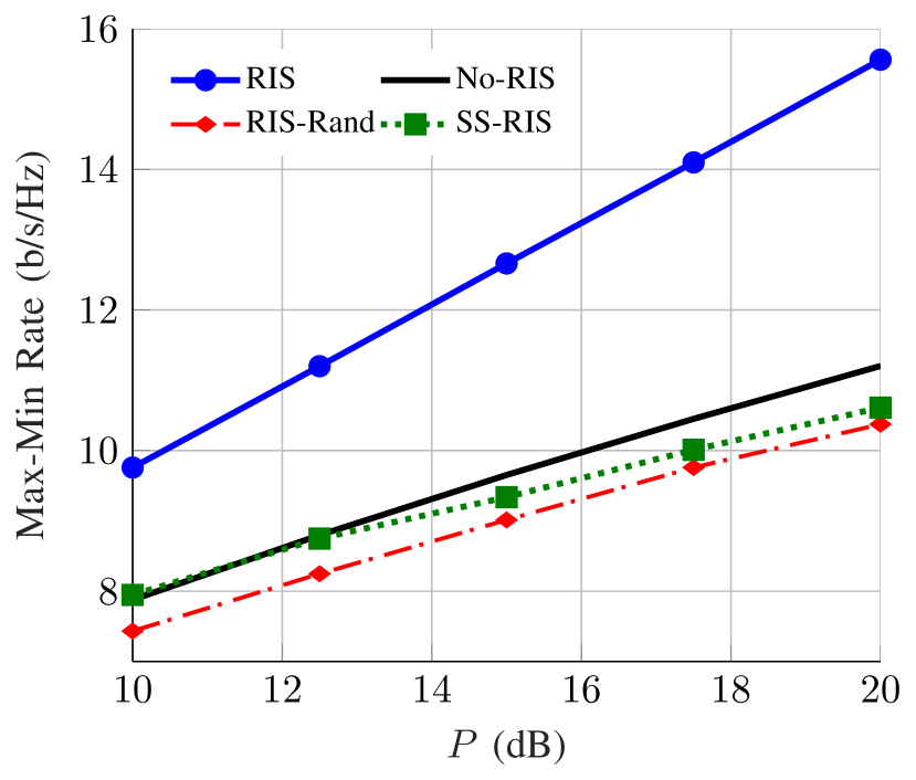
(a) Average max-min rate.

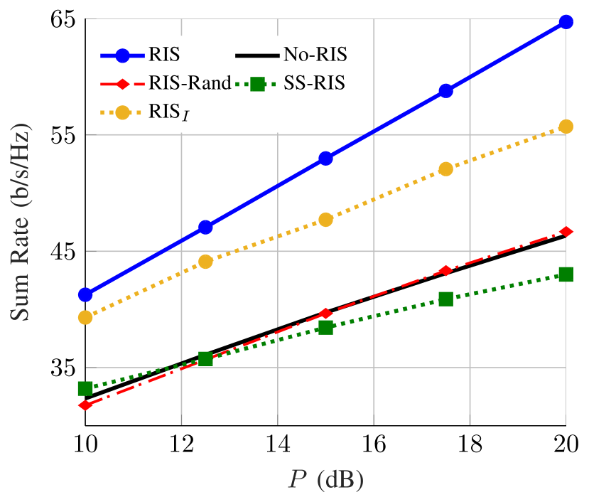
(b) Average sum rate.

Figure 2: Spectral efficiency metrics versus $P$ for $N_{{BS}}=4$, $N_{u}=4$, $K=2$, $L=2$, $M=2$, $n_{t}=256$, $\epsilon=10^{-5}$, and $N_{{RIS}}=20$.

Here, we present numerical results for SE maximization. To this end, we consider the maximum of the average minimum rate and the average sum rate of users as performance metrics. We refer to the maximum of the minimum achievable rate of users as the max-min rate. Note that it is likely that all the users get the same achievable rate when maximizing the minimum rate, which can provide a reasonable fairness among the users [46]. Nevertheless, when the sum rate is maximized, it could be the case that the users with weaker channels are switched off if QoS constraints are not considered. To provide a comprehensive analysis, we explore the impact of various parameters on the system performance, including the BS power budgets, packet length, as well as the maximum tolerable packet error rate.

IV-A1 Impact of power budget

In Fig. 2, we show the average max-min rate and sum rate versus $P$ for $N_{{BS}}=4$, $N_{u}=4$, $K=2$, $L=2$, $M=2$, $n_{t}=256$, $\epsilon=10^{-5}$, and $N_{{RIS}}=20$. In this figure, the RISs significantly improve the min-max rate and the sum rate, when the RIS elements are optimized. Surprisingly, employing RISs with random elements degrades the max-min rate. Moreover, we can observe that the benefits of RIS increase with $P$ in these examples. Additionally, the multi-stream scheme substantially improves the SE in these two examples.

IV-A2 Impact of packet length

(a) Average max-min rate.

(b) Average performance improvement.

Figure 3: Average max-min rate and relative performance improvement by RIS versus $n_{t}$ for $P=10$ dB, $N_{{BS}}=4$, $N_{u}=3$, $K=2$, $L=2$, $M=2$, $\epsilon=10^{-5}$, and $N_{{RIS}}=20$.

Fig. 3 shows the average max-min rate and the relative performance improvement by RIS versus $n_{t}$ for $P=10$ dB, $N_{{BS}}=4$, $N_{u}=3$, $K=2$, $L=2$, $M=2$, $\epsilon=10^{-5}$, and $N_{{RIS}}=20$. Observe that a RIS can substantially increase the average max-min rate. The benefits of deploying RISs decrease with $n_{t}$. Indeed, the shorter the packet length is, the higher the relative improvements provided by RISs can be. As indicated, the packet length correlates with the level of stringency in the latency constraint. Shorter packet lengths are needed, when the latency constraint is more stringent. Thus, this result shows that the RIS benefits increase as the latency constraint becomes more stringent. In other words, RISs can even be more beneficial for URLLC systems. Moreover, the rates increase with $n_{t}$ and converge to the Shannon rate when $n_{t}$ becomes higher. Furthermore, we can observe that employing multi-stream data transmission substantially increases the average max-min rate for all the values of $n_{t}$.

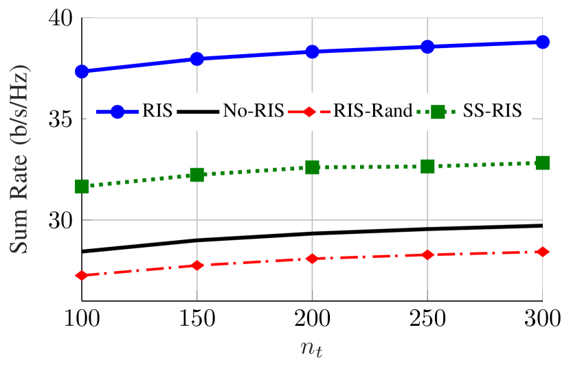
(a) $N_{{BS}}=4$, $N_{u}=3$, $K=2$, and $N_{{RIS}}=20$.

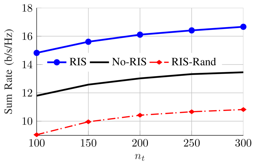
(b) $N_{{BS}}=2$, $N_{u}=2$, $K=4$, and $N_{{RIS}}=60$.

Figure 4: Average sum rate versus $n_{t}$ for $P=10$ dB, $L=2$, $M=2$, and $\epsilon=10^{-5}$.

Fig. 4 shows the average sum rate versus $n_{t}$ for $P=10$ dB, $L=2$, $M=2$, $\epsilon=10^{-5}$ and for different values of $N_{BS}$, $N_{u}$, $K$ and $N_{RIS}$. In this figure, RISs substantially enhance the average sum rate. However, the benefits of RISs are much more significant when there are less users in the system (Fig. 4a). Moreover, we can observe that the impact of decreasing the packet length is more severe in the system for a higher number of users. This may show the importance of employing effective interference-management techniques, which should be addressed in future studies. In Fig. 4a, we also observe that the algorithm conceived for the multi-stream data transmission per user outperforms the beamforming scheme, which employs a single-stream data transmission.

IV-A3 Impact of the reliability constraint

(a) Average max-min rate.

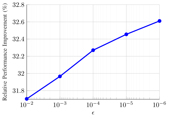
(b) Average performance improvement.

Figure 5: Average max-min rate and relative performance improvement by RIS versus $\epsilon$ for $P=10$ dB, $N_{{BS}}=4$, $N_{u}=3$, $K=2$, $L=2$, $M=2$, $n_{t}=256$ bits, and $N_{{RIS}}=20$.

Fig. 5 shows the average max-min rate and relative performance improvement enabled by the deployment of RISs versus $\epsilon$ for $P=10$ dB, $N_{{BS}}=4$, $N_{u}=3$, $K=2$, $L=2$, $M=2$, $n_{t}=256$ bits, and $N_{{RIS}}=20$. In this example, RIS significantly enhances the average max-min rate for all the $\epsilon$ considered. As expected, the average max-min rate decreases when the reliability constraint is more stringent. In other words, we have to transmit at a lower rate to reduce the decoding error rate. Moreover, the multi-stream scheme significantly outperforms the single-stream data transmission. Furthermore, we can observe in Fig. 5b that the benefits of RIS increase when $\epsilon$ decreases. Thus, RISs can be even more beneficial when more reliable communication is required.

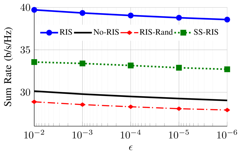
(a) $N_{{BS}}=4$, $N_{u}=3$, $K=2$, and $N_{{RIS}}=20$.

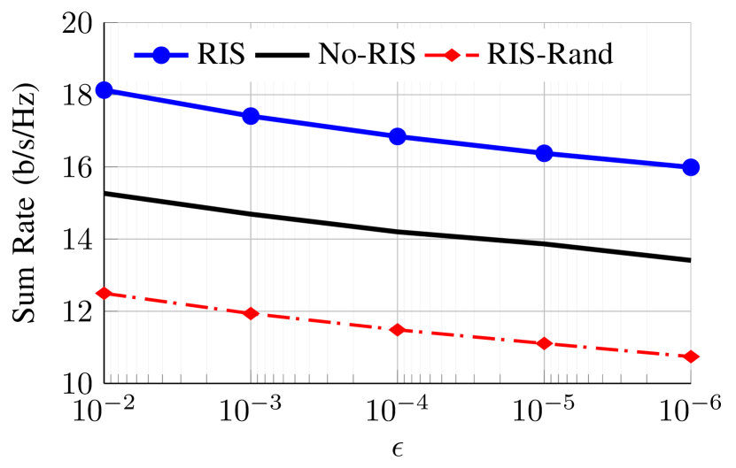
(b) $N_{{BS}}=2$, $N_{u}=2$, $K=4$, and $N_{{RIS}}=60$.

Figure 6: Average sum rate versus $\epsilon$ for $P=10$ dB, $L=2$, $M=2$, and $n_{t}=256$ bits.

Fig. 6 shows the average sum rate versus $\epsilon$ for $P=10$ dB, $L=2$, $M=2$, $n_{t}=256$ bits and different $N_{BS}$, $N_{u}$, $K$ and $N_{RIS}$. As it can be observed, RISs enhance the average sum rate in both networks, if the RIS elements are optimized. However, RISs with random coefficients decrease the average sum rate in these two examples. We can also observe that the impact of varying $\epsilon$ is higher in the system supporting more users. Additionally, we can note a significantly greater advantage from RISs when there are fewer users in the network. Moreover, we can observe that the average sum rate substantially increases, if we employ multi-stream data transmission.

IV-A4 Comparison of reflective RIS and STAR-RIS

Figure 7: Average max-min rate versus $P$ for $N_{{BS}}=2$, $N_{u}=2$, $K=2$, $L=1$, $M=1$, $\epsilon=10^{-5}$, $n_{t}=256$ bits and $N_{{RIS}}=40$.

A reflective RIS has the same performance as a STAR-RIS if all the users are in the reflection half-space of the reflective/STAR-RIS. Thus, to evaluate the performance differences between these two technologies, we consider a single-cell $2\times 2$ MIMO BC in which one of the users is in the reflection space, and the other one is in the transmission space. As shown in Fig. 7, STAR-RIS using the MS scheme can significantly outperform reflective RIS in this example. For instance, STAR-RIS provides about $25\%$ higher average max-min rate at $P=10$ dB compared to the reflective RIS.

IV-B Energy Efficiency Metrics

Now we investigate the EE of RIS in MU-MIMO URLLC BCs. To this end, we consider the impact of $P_{c}$, $\epsilon$, and $n_{t}$. In the examples provided in this subsection, we assume that each RIS consumes $1$ W power. Thus, to make a fair comparison, we consider a lower constant power ($P_{c}$) for the systems operating without RISs. Moreover, we assume that the power budget of the BSs is $P=10$ dB.

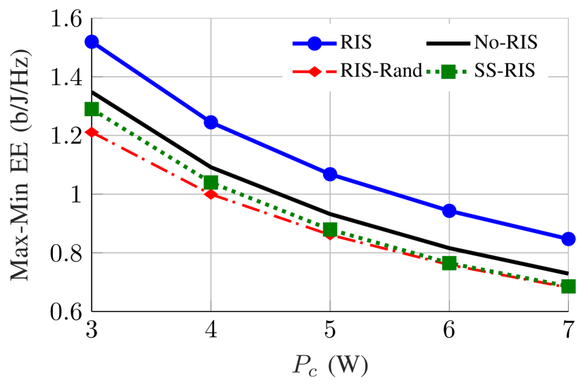
(a) Average max-min EE.

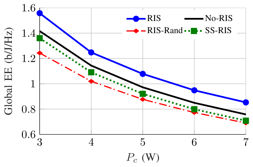
(b) Average global EE.

Figure 8: Energy efficiency metrics versus $P_{c}$ for $N_{{BS}}=5$, $N_{u}=5$, $K=2$, $L=2$, $M=2$, $n_{t}=256$, $\epsilon=10^{-5}$, and $N_{{RIS}}=20$.

IV-B1 Impact of $P_{c}$

Fig. 8 shows the average max-min EE and GEE versus $P_{c}$ for $N_{{BS}}=5$, $N_{u}=5$, $K=2$, $L=2$, $M=2$, $n_{t}=256$ bits, $\epsilon=10^{-5}$, and $N_{{RIS}}=20$. Note that we use the term max-min EE to refer to the highest minimum EE. As it can be observed, RISs significantly increase the average max-min EE and GEE with FBL. Interestingly, RISs may reduce the EE, if their elements are random. However, our proposed algorithms can statistically enhance the EE of RIS-aided scenarios. For instance, in the particular example of Fig. 8a, a RIS provides more than $10\%$ improvements over the systems disregarding the RISs for all the values of $P_{c}$ considered. Additionally, the multi-stream scheme significantly outperforms the single-stream data transmission in the both examples.

IV-B2 Impact of the reliability constraint

Figure 9: Average max-min EE versus $\epsilon$ for $P=10$ dB, $N_{{BS}}=4$, $N_{u}=4$, $K=2$, $L=1$, $M=1$, $n_{t}=256$ bits, and $N_{{RIS}}=20$.

Fig. 9 shows the average max-min EE versus $\epsilon$ for $P=10$ dB, $N_{{BS}}=4$, $N_{u}=4$, $K=2$, $L=1$, $M=1$, $n_{t}=256$ bits, and $N_{{RIS}}=20$. In this example, the RIS providea a significant gain, which increases with $\epsilon$. Again, RIS decreases the max-min EE when its elements are random. Moreover, we can observe that single-stream data transmission is suboptimal in this $4\times 4$ MIMO system. Indeed, the multi-stream systems communicating without RIS outperforms the RIS-aided single-stream data transmission.

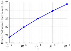
Figure 10: Average EE performance improvement by RIS versus $\epsilon$ for $P=10$ dB, $N_{{BS}}=2$, $N_{u}=2$, $K=2$, $L=2$, $M=2$, $n_{t}=256$ bits, and $N_{{RIS}}=20$.

Fig. 10 shows the average EE performance improvement attained by RISs versus $\epsilon$ for $P=10$ dB, $N_{{BS}}=2$, $N_{u}=2$, $K=2$, $L=2$, $M=2$, $n_{t}=256$ bits, and $N_{{RIS}}=20$. In this example, the RIS substantially increases the average max-min for all values of $\epsilon$. Moreover, higher gains are achieved by RISs, when the tolerable bit error rate is lower. Thus, the more reliable the communication has to be, the more energy efficient the RIS-aided systems becomes.

IV-B3 Impact of the packet length

Figure 11: Average max-min EE versus $n_{t}$ for $P=10$ dB, $N_{{BS}}=4$, $N_{u}=4$, $K=2$, $L=1$, $M=1$, $\epsilon=10^{-5}$, and $N_{{RIS}}=20$.

Fig. 11 shows the average max-min EE versus $n_{t}$ for $P=10$ dB, $N_{{BS}}=4$, $N_{u}=4$, $K=2$, $L=1$, $M=1$, $\epsilon=10^{-5}$, and $N_{{RIS}}=20$. In this figure, RIS provides a significant gain when the RIS elements are optimized by our proposed algorithm. However, random RIS coefficients degrade the EE performance.

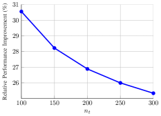
Figure 12: Average EE performance improvement by RIS versus $n_{t}$ for $P=10$ dB, $N_{{BS}}=2$, $N_{u}=2$, $K=2$, $L=2$, $M=2$, $\epsilon=10^{-5}$, and $N_{{RIS}}=20$.

Fig. 12 shows the average EE improvement by RISs versus $n_{t}$ for $P=10$ dB, $N_{{BS}}=2$, $N_{u}=2$, $K=2$, $L=2$, $M=2$, $\epsilon=10^{-5}$, and $N_{{RIS}}=20$. The average improvements reduce as $n_{t}$ increases. This indicates that the lower the tolerable latency is, the higher gain the RIS can provide. In other words, RIS-aided systems become more energy efficient when a low latency is required, as in control channels, for example.

V Summary and Conclusions

An optimization framework was proposed for MU-MIMO RIS-aided systems with FBL by considering the NA for the rate expressions. To this end, we first calculated closed-form expressions for the FBL rate and then obtained suitable concave lower bounds for the FBL rates. Our proposed framework can be adapted to any MU-MIMO system in which interference is treated as noise. Moreover, the framework can obtain a stationary point of a broad spectrum of practical optimization problems such as the maximization of the minimum/sum rate, GEE and minimum EE, when the set of the feasible RIS coefficients adheres to convexity. In summary, the key conclusions of this work are:

• RISs may significantly increase the average max-min rate, sum rate, max-min EE and global EE of the MU-MIMO systems considered. However, the RIS elements should be optimized to attain the above benefits, since RISs utilizing random elements may even degrade the system performance.

• The benefits of RISs increase when the packet lengths are reduced and/or the tolerable bit error rate is lower. The packet length can be related to the latency constraint, and the tolerable bit error rate represents the reliability constraint. Thus, these results show that RISs can be even more beneficial in URLLC systems than in non-URLLC systems.

• Multiple-stream data transmission for each user significantly outperforms single-stream data transmission (beamforming) in MU-MIMO RIS-assisted URLLC systems. Indeed, both the reliability and latency can be enhanced, when multiple-stream data transmission is employed in multiple-antenna systems.

In future research, it would be interesting to develop advanced interference-management techniques such as RSMA and NOMA for MU-MIMO URLLC BCs. Moreover, studying the performance of other concepts/technologies for RIS, such as holographic RIS, active RIS, and BD-RIS, can be another promising direction for extending this work.

References

- [1] C.-X. Wang et al., “On the road to 6G: Visions, requirements, key technologies and testbeds,” IEEE Commun. Surv. Tutor., , vol. 25, no. 2, pp. 905–974, 2023.
- [2] T. Gong et al., “Holographic MIMO communications: Theoretical foundations, enabling technologies, and future directions,” IEEE Commun. Surv. Tutor., doi: 10.1109/COMST.2023.3309529, 2023.
- [3] Q. Wu et al., “Intelligent reflecting surface aided wireless communications: A tutorial,” IEEE Trans. Commun., vol. 69, no. 5, pp. 3313–3351, 2021.
- [4] M. Di Renzo et al., “Smart radio environments empowered by reconfigurable intelligent surfaces: How it works, state of research, and the road ahead,” IEEE J. Sel. Areas Commun., vol. 38, no. 11, pp. 2450–2525, 2020.
- [5] C. Huang et al., “Reconfigurable intelligent surfaces for energy efficiency in wireless communication,” IEEE Trans. Wireless Commun., vol. 18, no. 8, pp. 4157–4170, 2019.
- [6] Q. Wu and R. Zhang, “Intelligent reflecting surface enhanced wireless network via joint active and passive beamforming,” IEEE Trans. Wireless Commun., vol. 18, no. 11, pp. 5394–5409, 2019.
- [7] Q.-U.-A. Nadeem, et al., “Asymptotic max-min SINR analysis of reconfigurable intelligent surface assisted MISO systems,” IEEE Trans. Wireless Commun., vol. 19, no. 12, pp. 7748–7764, 2020.
- [8] M. Soleymani, I. Santamaria, E. Jorswieck, and S. Rezvani, “NOMA-based improper signaling for multicell MISO RIS-assisted broadcast channels,” IEEE Trans. Signal Process., vol. 71, pp. 963–978, March 2023.
- [9] I. Santamaria, M. Soleymani, E. Jorswieck, and J. Gutierrez, “Interference leakage minimization in RIS-assisted MIMO interference channels,” Proc. IEEE Int. Conf. on Acoust., Speech and Signal Processing (ICASSP), pp. 1–5, 2023.
- [10] M. Soleymani, I. Santamaria, A. Sezgin, and E. Jorswieck, “Maximization of minimum rate in MIMO OFDM RIS-assisted broadcast channels,” IEEE Int. Workshop Comput. Adv. Multi-Sensor Adaptive Process. (CAMSAP), pp. 11–15, 2023.
- [11] M. Soleymani, I. Santamaria, and E. Jorswieck, “Spectral and energy efficiency maximization of MISO STAR-RIS-assisted URLLC systems,” IEEE Access, vol. 11, pp. 70833–70852, 2023.
- [12] M. Soleymani, I. Santamaria, E. Jorswieck, and B. Clerckx, “Optimization of rate-splitting multiple access in beyond diagonal RIS-assisted URLLC systems,” IEEE Trans. Wireless Commun., , doi: 10.1109/TWC.2023.3324190, 2023.
- [13] Y. Li, C. Yin, T. Do-Duy, A. Masaracchia, and T. Q. Duong, “Aerial reconfigurable intelligent surface-enabled URLLC UAV systems,” IEEE Access, vol. 9, pp. 140 248–140 257, 2021.
- [14] T.-H. Vu, T.-V. Nguyen, D. B. da Costa, and S. Kim, “Intelligent reflecting surface-aided short-packet non-orthogonal multiple access systems,” IEEE Trans. Veh. Technol., vol. 71, no. 4, pp. 4500–4505, 2022.
- [15] H. Xie, J. Xu, Y.-F. Liu, L. Liu, and D. W. K. Ng, “User grouping and reflective beamforming for IRS-aided URLLC,” IEEE Wireless Commun. Lett., vol. 10, no. 11, pp. 2533–2537, 2021.
- [16] M. Almekhlafi, M. A. Arfaoui, M. Elhattab, C. Assi, and A. Ghrayeb, “Joint resource allocation and phase shift optimization for RIS-aided eMBB/URLLC traffic multiplexing,” IEEE Trans. Commun., vol. 70, no. 2, pp. 1304–1319, 2022.
- [17] W. R. Ghanem, V. Jamali, and R. Schober, “Optimal resource allocation for multi-user OFDMA-URLLC MEC systems,” IEEE Open J. Commun. Soc., vol. 3, pp. 2005–2023, 2022.
- [18] B. Makki, T. Svensson, M. Coldrey, and M.-S. Alouini, “Finite block-length analysis of large-but-finite MIMO systems,” IEEE Wireless Commun. Lett., vol. 8, no. 1, pp. 113–116, Feb. 2019.
- [19] B. Makki, T. Svensson, T. Eriksson, and M.-S. Alouini, “On the required number of antennas in a point-to-point large-but-finite MIMO system: Outage-limited scenario,” IEEE Trans. Commun., vol. 64, no. 5, pp. 1968–1983, May 2016.
- [20] C. Li, Y. Wang, W. Chen, and H. V. Poor, “Ultra-reliable and low-latency multiple-antenna communications in the high SNR regime,” IEEE Wireless Commun. Lett., vol. 12, no. 3, pp. 461–465, March 2023.
- [21] Y. Polyanskiy, H. V. Poor, and S. Verdú, “Channel coding rate in the finite blocklength regime,” IEEE Trans. Inf. Theory, vol. 56, no. 5, pp. 2307–2359, 2010.
- [22] T. Erseghe, “Coding in the finite-blocklength regime: Bounds based on laplace integrals and their asymptotic approximations,” IEEE Trans. Inf. Theory, vol. 62, no. 12, pp. 6854–6883, 2016.
- [23] ——, “On the evaluation of the Polyanskiy-Poor–Verdú converse bound for finite block-length coding in AWGN,” IEEE Trans. Inf. Theory, vol. 61, no. 12, pp. 6578–6590, 2015.
- [24] Y. Polyanskiy, Channel coding: Non-asymptotic fundamental limits. Ph.D. dissertation, Dept. Electr. Eng., Princeton Univ., Princeton, NJ, USA, Nov. 2010.
- [25] M. Soleymani, I. Santamaria, and P. J. Schreier, “Improper signaling for multicell MIMO RIS-assisted broadcast channels with I/Q imbalance,” IEEE Trans. Green Commun. Netw., vol. 6, no. 2, pp. 723–738, 2022.
- [26] M. Soleymani, I. Santamaria, and E. Jorswieck, “Rate region of MIMO RIS-assisted broadcast channels with rate splitting and improper signaling,” WSA 2023; 26th International ITG Workshop on Smart Antennas, pp. 1–6, 2023.
- [27] J. Scarlett, V. Y. Tan, and G. Durisi, “The dispersion of nearest-neighbor decoding for additive non-Gaussian channels,” IEEE Trans. Inf. Theory, vol. 63, no. 1, pp. 81–92, 2016.
- [28] M. Abughalwa, H. Tuan, D. Nguyen, H. Poor, and L. Hanzo, “Finite-blocklength RIS-aided transmit beamforming,” IEEE Trans. Veh. Technol., vol. 71, no. 11, pp. 12 374–12 379, 2022.
- [29] W. R. Ghanem, V. Jamali, and R. Schober, “Joint beamforming and phase shift optimization for multicell IRS-aided OFDMA-URLLC systems,” in IEEE Wireless Commun. and Netw. Conf. (WCNC), pp. 1–7, 2021.
- [30] H. Ren, K. Wang, and C. Pan, “Intelligent reflecting surface-aided URLLC in a factory automation scenario,” IEEE Trans. Commun., vol. 70, no. 1, pp. 707–723, 2021.
- [31] B. Zhang, K. Wang, K. Yang, and G. Zhang, “IRS-assisted short packet wireless energy transfer and communications,” IEEE Wireless Commun. Lett., vol. 11, no. 2, pp. 303–307, 2022.
- [32] C. Pan, H. Ren, K. Wang, W. Xu, M. Elkashlan, A. Nallanathan, and L. Hanzo, “Multicell MIMO communications relying on intelligent reflecting surfaces,” IEEE Trans. Wireless Commun., vol. 19, no. 8, pp. 5218–5233, 2020.
- [33] H. Yu et al., “Joint design of reconfigurable intelligent surfaces and transmit beamforming under proper and improper Gaussian signaling,” IEEE J. Sel. Areas Commun., vol. 38, no. 11, pp. 2589–2603, 2020.
- [34] L. Zhang, Y. Wang, W. Tao, Z. Jia, T. Song, and C. Pan, “Intelligent reflecting surface aided MIMO cognitive radio systems,” IEEE Trans. Veh. Technol., vol. 69, no. 10, pp. 11 445–11 457, 2020.
- [35] H. Zhang and B. Di, “Intelligent omni-surfaces: Simultaneous refraction and reflection for full-dimensional wireless communications,” IEEE Commun. Surv. Tutor., vol. 24, no. 4, pp. 1997–2028, 2022.
- [36] Y. Liu, X. Mu, J. Xu, R. Schober, Y. Hao, H. V. Poor, and L. Hanzo, “STAR: Simultaneous transmission and reflection for 360 coverage by intelligent surfaces,” IEEE Wireless Commun., vol. 28, no. 6, pp. 102–109, 2021.
- [37] X. Mu, Y. Liu, L. Guo, J. Lin, and R. Schober, “Simultaneously transmitting and reflecting (STAR) RIS aided wireless communications,” IEEE Trans. Wireless Commun., vol. 21, no. 5, pp. 3083–3098, 2022.
- [38] M. Soleymani, I. Santamaria, A. Sezgin, and E. Jorswieck, “Maximizing spectral and energy efficiency in multi-user MIMO OFDM systems with RIS and hardware impairment,” arXiv preprint arXiv:2401.11921, 2024.
- [39] M. Soleymani, I. Santamaria, and E. Jorswieck, “Energy-efficient rate splitting for MIMO STAR-RIS-assisted broadcast channels with I/Q imbalance,” Proc. IEEE Eu. Signal Process. Conf. (EUSIPCO), pp. 1504–1508, 2023.
- [40] ——, “NOMA-based improper signaling for MIMO STAR-RIS-assisted broadcast channels with hardware impairments,” IEEE Global Commun. Conf. (GLOBECOM), 2023.
- [41] J. Xu, Y. Liu, X. Mu, R. Schober, and H. V. Poor, “STAR-RISs: A correlated TR phase-shift model and practical phase-shift configuration strategies,” IEEE J. Sel. Topics Signal Process., pp. 1–1, 2022.
- [42] A. Zappone and E. Jorswieck, “Energy efficiency in wireless networks via fractional programming theory,” Found Trends® in Commun. Inf. Theory, vol. 11, no. 3-4, pp. 185–396, 2015.
- [43] M. Soleymani, I. Santamaria, and E. Jorswieck, “Rate splitting in MIMO RIS-assisted systems with hardware impairments and improper signaling,” IEEE Trans. Veh. Technol., vol. 72, no. 4, pp. 4580–4597, April 2023.
- [44] Y. Sun, P. Babu, and D. P. Palomar, “Majorization-minimization algorithms in signal processing, communications, and machine learning,” IEEE Trans. Signal Process., vol. 65, no. 3, pp. 794–816, 2017.
- [45] S. Boyd and L. Vandenberghe, Convex Optimization. Cambridge University Press, 2004.
- [46] M. Soleymani et al., “Improper Gaussian signaling for the -user MIMO interference channels with hardware impairments,” IEEE Trans. Veh. Technol., vol. 69, no. 10, pp. 11 632–11 645, 2020.