Achievable Rate Optimization for Stacked Intelligent Metasurface-Assisted Holographic MIMO Communications

Abstract

Stacked intelligent metasurfaces (SIM) is a revolutionary technology, which can outperform its single-layer counterparts by performing advanced signal processing relying on wave propagation. In this work, we exploit SIM to enable transmit precoding and receiver combining in holographic multiple-input multiple-output (HMIMO) communications, and we study the achievable rate by formulating a joint optimization problem of the SIM phase shifts at both sides of the transceiver and the covariance matrix of the transmitted signal. Notably, we propose its solution by means of an iterative optimization algorithm that relies on the projected gradient method, and accounts for all optimization parameters simultaneously. We also obtain the step size guaranteeing the convergence of the proposed algorithm. Simulation results provide fundamental insights such the performance improvements compared to the single-RIS counterpart and conventional MIMO system. Remarkably, the proposed algorithm results in the same achievable rate as the alternating optimization (AO) benchmark but with a less number of iterations.

I Introduction

The need for sixth-generation (6G) cellular networks has appeared on the horizon of the wireless network evolution [1]. Their extreme targets require vast improvements on data rates and latency together with wider connectivity to cover the explosive proliferation of the Internet-of-Everything (IoE), such as virtual/augmented reality (VR/AR) and the increase in connected devices. In particular, the latter is expected to reach $500$ million by $2030$ [2]. Various technologies such as massive multiple-input multiple-output (mMIMO) and millimeter wave (mmWave) communications that have been suggested in recent years that require low energy consumption and can achieve high data rates, but they concern transceiver features without being able to shape the propagation channel with its stochastic characteristics that limit the performance [3].

Two possible approaches that solve the aforementioned issues are the proposed 6G-enabled technologies, reconfigurable intelligent surfaces (RIS) [4, 5, 6, 7], and holographic multiple-input multiple-output (HMIMO) Communications [8]. Specifically, RIS and its various equivalents have been proposed to realize smart reconfigurable environments [4]. A RIS is a planner metasurface equipped with a large number of nearly passive elements that induce phase shifts and/or amplitude attenuation to the impinging waves through a smart controller. Also, optimization of the reflected signals enable us to control the interaction of the reflection characteristics with the surrounding objects. RIS performance gains have been studied under various system and channel setups, but most works have focused on single-input single-output (SISO) or multiple-input single-output (MISO) systems with single-antenna receivers [9, 10, 11, 12, 6, 13, 14, 15, 16], while the research on RIS-assisted MIMO assisted is limited [17, 18]. In particular, the study of the capacity limit of RIS-assisted MIMO systems requires the joint optimization of the RIS phase shifts and MIMO transmit covariance matrix [19, 20]. It is worthwhile to mention that since RISs do not require active transmitter radio frequency (RF) chains, they can be densely implemented with low energy consumption and low cost [5]. However, single-layer RIS designs are not capable of implementing advanced MIMO functionalities because of hardware limitations and suffer from severe path-loss attenuation.

On the ground of mMIMO systems with its improvements on spectral and energy efficiencies and their other benefits such as reduced latency [21], HMIMO has emerged as a new concept describing possibly the next MIMO generation [8, 22]. For example, in [23], a large intelligent surface (LIS) including a massive number of elements it was shown that great improvements are expected. The fundamental limits of HMIMO systems were characterised in [24] by suggesting correlated random Gaussian fading for the far field. In the case of arbitrary scattering environments a Fourier plane-wave series-based expansion of the HMIMO channel response was developed in [25]. In [26], a channel estimation scheme was proposed for arbitrary spatial correlation matrices. However, HMIMO have the disadvantages of excessive hardware cost and energy consumption because they are implemented by a large number of active components.

Recently, not only stacked intelligent metasurfaces (SIMs) have been proposed where multiple surfaces are cascaded [27, 28], but SIMs were integrated with the transceiver to implement HMIMO communications in [29]. It was shown that a SIM can implement signal processing in the electromagnetic (EM) wave regime. The motivation behind this work was to substitute the exprensive active elements at the tranceiver by exploiting the technology of programmable metasurfaces. In [23, 8], single-layer surfaces were used but the multilayer surface design is more advantageous for enhancing the spatial-domain gain by forming diverse waveforms with high accuracy.

From theoretical and practical standpoints, it is crucial to optimise the achievable rate for RIS-assisted systems. Hence, various optimization methods have been suggested in prior works, which aim to find near-optimal solutions obeying to reasonable run time and computational complexity. Most of these works considered single-antenna receive devices and relied on the alternating optimization (AO) method which optimises the transmit beamformer and the RIS phase shifts in an alternating way [12, 6]. For example, in [12], the gradient method was employed in an AO fashion to optimize the phase shifts. Other examples of AO-based works on RIS-assisted MIMO communication are [30, 31, 19, 20]. In [30], a RIS was optimized to increase the rank of the channel matrix. In [31], the optimization took place in an indoor mmWave environment. Moreover, in [19], the achievable rate of RIS-assisted multi-stream MIMO was maximized by using the AO method. However, AO-based methods require possibly many iterations to converge, which increase with the size of the RIS. Note that this is the case, where a RIS is more beneficial in practice. Contrary to this background, a joint optimization of the RIS elements and the transmit covariance matrix in [20], where an iterative projected gradient method was proposed.

Contributions: Motivated by the above observations, the topic of this paper concerns the study of SIM-enabled HMIMO systems by optimising simultaneously all parameters of the joint optimization problem to reduce the convergence time compared to an AO approach. Contrary to [29], which considers a full analog SIM-enabled HMIMO architecture by means of an AO approach we focus on a more general hybrid digital and wave design that also applies a more efficient algorithm optimizing all relevant parameters simultaneously. Compared to [20] and [14], which assumed a conventional RIS-assisted system and a STAR-RIS system, where two parameters are optimized simultaneously, we consider a general SIM-enabled system, where we optimize three key parameters simultaneously. Our main contributions are summarised as follows.

• We maximise the achievable rate of a multi stream HMIMO system equipped with a SIM at the transmitter and a SIM at the receiver. To this end, we formulate the joint optimization problem of the transmit covariance matrix, and the RIS phase shift values of each surface at the transmitter and the receiver SIMs.

• We propose an iterative projected gradient approach, which solves the underlying nonconvex problem. Also, we derive the gradients and the projection expressions for all parameters in closed-forms. Moreover, we show that the proposed approach converges to a critical point.

• We determine the appropriate step size that makes the proposed algorithm to converge by deriving first the Lipschitz constant.

• Simulation and analytical results coincide and show that both the proposed approach and the AO method result in the same rate but our approach achieves it with a substantially lower number of iterations. Furthermore, the proposed approach has remarkably lower computational complexity with respect to the AO method.

Paper Outline: The structure of this papers follows. Section II presents the system model and the problem formulation of a SIM-assisted HMIMO system. Section III presents the simultaneous optimization of the achievable rate with respect to all its parameters. Section LABEL:convergence provides the convergence and complexity analyses. In Section LABEL:Numerical, we provide the numerical results, and Section VI concludes the paper.

Notation: Vectors and matrices are denoted by boldface lower and upper case symbols, respectively. The notations $(\cdot)^{\scriptscriptstyle\mathsf{T}}$, $(\cdot)^{\scriptscriptstyle\mathsf{H}}$, and $\tr\!\left({\cdot}\right)$ describe the transpose, Hermitian transpose, and trace operators, respectively. Moreover, the notations $\arg\left(\cdot\right)$ and $\mathbb{E}\left[\cdot\right]$ express the argument function and the expectation operator, respectively. The notation $\text{diag}\left(\right)\left({\mathbf{A}}\right)$ describes a vector with elements equal to the diagonal elements of ${\mathbf{A}}$, the notation $\text{diag}\left(\right)\left({\mathbf{x}}\right)$ describes a diagonal matrix whose elements are ${\mathbf{x}}$, while ${\mathbf{b}}\sim{\cal C}{\cal N}{({\mathbf{0}},\mathbf{\Sigma})}$ describes a circularly symmetric complex Gaussian vector with zero mean and a covariance matrix $\mathbf{\Sigma}$.

II System Model and Problem Formulation

II-A System Model

We consider a SIM-assisted HMIMO, where the transmitter and the receiver have $N_{t}$ and $N_{r}$ antennas, respectively, while each of them is assisted by a SIM as shown in Fig. 1. Specifically, each SIM consists of a closed vacuum container having several stacked metasurface layers [27]. The operation requires a customized field programmable gate array (FPGA), or generally a smart controller, which can adjust the phase shift of the EM waves impinging on each meta-atom. Hence, a customized spatial waveform shape at the output of each metasurface layer is automatically produced as the transmit signals propagate through the SIM. The EM waves can be transmitted from the output metasurface of the transmitter SIM into the ether, and then, acquired by the receiver SIM, i.e., HMIMO communication can be supported while by leveraging the SIM-based analog beamforming to approach its digital counterpart. In particular, the transmitter SIM plays the role of the precoder by sending the information-bearing EM wave through the ether to the receiver SIM, which can combine the received EM to recover the transmitted signal. In other words, precoding and combining take place partially in the wave domain [29].

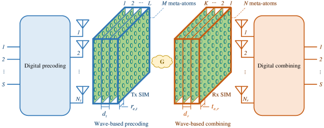
Figure 1: A SIM-assisted HMIMO system.

According to Fig. 1, which illustrates the SIM-assisted HMIMO system supporting precoding and combining in the wave domain, we rely on the SIM design proposed in [29]. Specifically, we denote $L$ the number of metasurface layers at the transmitter and $K$ the number of metasurface layers at the receiver, while $\mathcal{L}=\{1,\ldots,L\}$ and $\mathcal{K}=\{1,\ldots,K\}$ represent their sets, respectively. Without any loss of generality, we assume that each metasurface layer at the transmitter and the receiver consists of an identical number of meta-atoms. In particular, we denote $M$ and $N$ the number of meta-atoms on each metasurface layer at the transmitter SIM and receiver SIM, respectively. The respective sets are denoted as $\mathcal{M}=\{1,\ldots,M\}$ and $\mathcal{N}=\{1,\ldots,N\}$. On this ground, we denote $\theta_{m}^{l}\in[0,2\pi),m\in\mathcal{M},l\in\mathcal{L}$ the phase shift by meta-atom $m$ on the transmit metasurface layer $l$ with $\phi_{m}^{l}=e^{j\theta_{m}^{l}}$ being the respective transmission coefficient. The transmission coefficient matrix, associated with the $l$-th transmit layer, is denoted by ${\bm{\Phi}}^{l}=\text{diag}\left(\right)({\bm{\phi}}^{l})\in\mathbb{C}^{M\times M}$, where ${\bm{\phi}}^{l}=[\phi^{l}_{1},\dots,\phi^{l}_{M}]^{{\scriptscriptstyle\mathsf{T}}}\in\mathbb{C}^{M\times 1}$. Similarly, we denote $\xi_{n}^{k}\in[0,2\pi),n\in\mathcal{N},k\in\mathcal{K}$ the phase shift by meta-atom $n$ on the receive metasurface layer $k$ with $\psi_{n}^{k}=e^{j\xi_{n}^{k}}$ being the corresponding transmission coefficient. The $k$-th receive coefficient matrix is denoted by ${\bm{\Psi}}^{k}=\text{diag}\left(\right)({\bm{\psi}}^{k})\in\mathbb{C}^{M\times N}$, where ${\bm{\psi}}^{k}=[\psi^{k}_{1},\dots,\psi^{k}_{M}]^{{\scriptscriptstyle\mathsf{T}}}\in\mathbb{C}^{N\times 1}$.

Remark 1

In this work, we assume continuously-adjustable phase shifts and constant modulus equal to $1$ to assess the performance of SIM-assisted HMIMO communications while maximizing the achievable rate as in [9]. Practical issues such as the assumption of coupled phase and magnitude [32] and the consideration of discrete phase shifts [27] will be studied in future work.

Remark 2

Note that our hybrid digital and wave architecture employing multiple-layer SIM significantly outperforms the conventional hybrid benchmarks whose performance is constrained by analog components, e.g., constant- modulus phase shifters. Remarkably, our hybrid architecture may approach the performance of an all-digital system, while the number of RF chains reduces from $M$ to $N_{t}$.

With all metasurface layers having an isomorphic lattice arrangement [27], we model each surface as a uniform planar array, where the element spacing between the $\tilde{m}$th and $m$th meta-atoms on the same transmit metasurface is given by [29]

$$r_{m,\tilde{m}}=r_{e,t}\sqrt{(m_{z}-\tilde{m}_{z})^{2}+(m_{x}-\tilde{m}_{x})^{2}}$$ (1)

with $r_{e,t}$ expressing the element spacing between adjacent meta-atoms on the same transmit metasurface. Moreover, $m_{x}$ and $m_{z}$ correspond to the $m$th meta-atom along the $x$-axis and the $z$-axis, respectively, which are given by

$$m_{x}=\!\!\!\!\!\mod(m-1,m_{\mathrm{max}})+1,~{}~{}~{}m_{z}=\lceil m/m_{\mathrm{max}}\rceil$$ (2)

with $m_{\mathrm{max}}$ being the highest number of meta-atoms included on each row of the transmit surface. In a similar way, the element spacing between the $n$th meta-atom and the $\tilde{n}$th one on the same receive metasurface can be described as

$$t_{\tilde{n},n}=t_{e,r}\sqrt{(\tilde{n}_{x}-n_{x})^{2}+(\tilde{n}_{z}-n_{z})^{2}},$$ (3)

where $t_{e,r}$ expresses the element spacing between adjacent meta-atoms on the same receive metasurface with $n_{x}$ and $n_{z}$ describing the indices of the $n$th meta-atom along the $x$-axis and the $z$-axis, respectively. These indices are given by

$$n_{x}=\!\!\!\!\!\mod(n-1,n_{\mathrm{max}})+1,~{}~{}~{}n_{z} =\lceil n/n_{\mathrm{max}}\rceil,$$ (4)

where $n_{\mathrm{max}}$ is the maximum number of meta-atoms on each row of the receive metasurface. For the sake of simplicity, we assume square surfaces at both the transmitter and receiver sides, i.e., $M=m_{\mathrm{max}}^{2}$ and $N=n_{\mathrm{max}}^{2}$.

By assuming uniform spacing among all surfaces and that all surfaces are parallel for the sake of simplicity, we define the transmission distance from meta-atom $\tilde{m}$ on the transmit metasurface $(l-1)$ to meta-atom $m$ on the transmit metasurface $l$ as

$$r_{m,\tilde{m}}^{l}=\sqrt{r_{m,\tilde{m}}^{2}+d_{t}^{2}},~{}l\ \in\mathcal{L}/\{1\},$$ (5)

where $d_{t}={D_{t}}/{L}$ is the spacing between any two adjacent metasurfaces at the transmitter SIM with $D_{t}$ describing the thickness of the transmitter SIM.

Similarly, we define the distance from meta-atom $\tilde{n}$ on the receive metasurface $k$ to meta-atom $\tilde{n}$ on the receive metasurface $(k-1)$ as

$$t_{\tilde{n},n}^{k}=\sqrt{d_{r}^{2}+t_{\tilde{n},n}^{2}},~{}k\ \in\mathcal{K}/\{1\},$$ (6)

where $d_{r}={D_{r}}/{L}$ is the spacing between any two adjacent metasurfaces at the receiver SIM with $D_{r}$ describing the thickness of the receiver SIM.

In addition, by assuming that the centers of the transmit and receive antenna arrays are aligned with the centers of all metasufaces while both antenna arrays are arranged in a uniform linear array with element spacing $\lambda/2$, the distances from the $s$th source to the $m$th meta-atom on the input metasurface of the transmitter SIM and from $n$th meta-atom on the output metasurface of the receiver SIM to the $s$th destination are provided by (7) and (8), respectively.

$$r_{m,s}^{1} =\sqrt{\left[\left(m_{z}-\frac{m_{\mathrm{max}+1}}{2}\right)r_{e,t}-\left(s-\frac{N_{t}+1}{2}\right)\frac{\lambda}{2}\right]^{2}+\left(m_{x}-\frac{m_{\mathrm{max}}+1}{2}\right)^{2}r_{e,t}^{2}+d_{t}^{2}},$$ (7)

$$t_{s,n}^{1} =\sqrt{\left[\left(n_{z}-\frac{n_{\mathrm{max}+1}}{2}\right)t_{e,r}-\left(s-\frac{N_{r}+1}{2}\right)\frac{\lambda}{2}\right]^{2}+\left(\frac{n_{\mathrm{max}}+1}{2}-n_{x}\right)^{2}t_{e,r}^{2}+d_{r}^{2}}.$$ (8)

II-B Channel Model

Regarding the transmission coefficient from meta-atom $\tilde{m}$ on the transmit metasurface layer $(l-1)$ to meta-atom $m$ on the transmit metasurface layer $l$, provided by the Rayleigh-Sommerfeld diffraction theory [33], it is given by

$$w_{m,\tilde{m}}^{l}=\frac{A_{t}cosx_{m,\tilde{m}}^{l}}{r_{m,\tilde{m}}^{l}}\left(\frac{1}{2\pi r^{l}_{m,\tilde{m}}}-j\frac{1}{\lambda}\right)e^{j2\pi r_{m,\tilde{m}}^{l}/\lambda},l\in\mathcal{L},$$ (9)

where $A_{t}$ denotes the meta-atom area at the transmitter SIM, $x_{m,\tilde{m}}^{l}$ is the angle between the propagation direction and the normal direction of the transmit metasurface layer $(l-1)$, and $r_{m,\tilde{m}}^{l}$, is the respective transmission distance. Hence, the effect of the transmitter SIM can be written as

$${\mathbf{P}}={\bm{\Phi}}^{L}{\mathbf{W}}^{L}\cdots{\bm{\Phi}}^{2}{\mathbf{W}}^{2}{\bm{\Phi}}^{1}{\mathbf{W}}^{1}\in\mathbb{C}^{M\times N_{t}},$$ (10)

where ${\mathbf{W}}^{l}\in\mathbb{C}^{M\times M},l\in\mathcal{L}/\{1\}$ is the transmission coefficient matrix between the transmit metasurface layer $(l-1)$ and the transmit metasurface layer $l$, while ${\mathbf{W}}^{1}\in\mathbb{C}^{M\times N_{t}}$ is the transmission coefficient matrix from the transmit antenna array to the input metasurface layer of the transmit SIM.

In the case of the transmission coefficient from meta-atom $n$ on the receive metasurface layer $k$ to the meta-atom $\tilde{n}$ on the receive metasurface layer $(k-1)$, it is given by

$$u_{\tilde{n},n}^{k}=\frac{A_{r}cos\zeta_{\tilde{n},n}^{k}}{t_{\tilde{n},n}^{k}}\left(\frac{1}{2\pi t^{k}_{\tilde{n},n}}-j\frac{1}{\lambda}\right)e^{j2\pi t_{\tilde{n},n}^{k}/\lambda},k\in\mathcal{K},$$ (11)

where $A_{r}$ is the meta-atom area in the receiver SIM, $\zeta_{\tilde{n},n}^{k}$ is the angle between the propagation direction and the normal direction of the receive metasurface layer $(k-1)$, and $t_{\tilde{n},n}^{k}$ is the corresponding transmission distance. Thus, the effect of the receiver SIM is expressed by

$${\mathbf{Z}}={\mathbf{U}}^{1}{\bm{\Psi}}^{1}{\mathbf{U}}^{2}{\bm{\Psi}}^{2}\cdots{\mathbf{U}}^{K}{\bm{\Psi}}^{K}\in\mathbb{C}^{N_{r}\times N},$$ (12)

where ${\mathbf{U}}^{k}\in\mathbb{C}^{N\times N},k\in\mathcal{K}/\{1\}$ is the transmission coefficient matrix between the receive metasurface layer $k$ to the receive metasurface layer $(k-1)$, and ${\mathbf{U}}^{1}\in\mathbb{C}^{N_{r}\times N}$ is the transmission coefficient matrix from the output metasurface layer of the receiver SIM to the receive antenna array.

Remark 3

Practical hardware imperfections such as innate modeling errors [27] may lead to deviation of the transmission coefficients between adjacent metasurface layers from those given by (9) and (11). In this case, calibration of these coefficients is necessary for each individual SIM. Although the calibration process is beyond the scope of this work, one solution suggests measuring the response at the receive panel after the transmission of a known signal as mentioned in [29]. Next, update of the transmission coefficients could take place after applying the standard error back-propagation algorithm [34].

Concerning the HMIMO channel between the transmitter and receiver SIMs, it is written as [35]

$${\mathbf{G}}={\mathbf{R}}^{1/2}_{\mathrm{R}}\tilde{{\mathbf{G}}}{\mathbf{R}}^{1/2}_{\mathrm{T}}\in\mathbb{C}^{N\times M},$$ (13)

where $\tilde{{\mathbf{G}}}\sim\mathcal{CN}({\mathbf{0}},\mathrm{PL}{\bm{\mathrm{I}}}_{N}\otimes{\bm{\mathrm{I}}}_{M})\in\mathbb{C}^{N\times M}$ denotes the independent and identically distributed (i.i.d.) Rayleigh fading channel, ${\mathbf{R}}_{\mathrm{T}}\in\mathbb{C}^{M\times M}$ is the spatial correlation matrix at the transmitter SIM, and ${\mathbf{R}}_{\mathrm{R}}\in\mathbb{C}^{N\times N}$ is the spatial correlation matrix at the receiver SIM. Note that $\mathrm{PL}$ corresponds to the average path loss between the transmitter and receiver SIMs. In particular, in the case of isotropic scattering and far-field propagation [24, 36], the spatial correlation matrices at the transmitter and receiver SIMs are given by [26]

$$[{\mathbf{R}}_{\mathrm{T}}]_{m,\tilde{m}} =\mathrm{sinc}(2r_{m,\tilde{m}}/\lambda),m\in\mathcal{M},\tilde{m}\in\mathcal{M},$$ (14)

$$[{\mathbf{R}}_{\mathrm{R}}]_{\tilde{n},n} =\mathrm{sinc}(2t_{\tilde{n},n}/\lambda),\tilde{n}\in\mathcal{N},n\in\mathcal{N},$$ (15)

respectively.

The path loss ,which attenuates the received signal is given by [37]

$$\mathrm{PL}(d)=\mathrm{PL}(d_{0})+10b\log_{10}\left(\frac{d}{d_{0}}\right)+X_{\delta},~{}d\geq d_{0},$$ (16)

where $X_{\delta}$ is a Gaussian random variable with a zero mean and a standard deviation $\delta$ that depends on shadow fading, $b$ is the path loss exponent, and $\mathrm{PL}(d_{0})=20\log_{10}(4\pi d_{0}/\lambda)~{}\mathrm{dB}$ denotes the free space path loss at the reference distance $d_{0}$.

The received signal vector at the destination is given by

$${\mathbf{y}}={\mathbf{H}}{\mathbf{x}}+{\mathbf{n}},$$ (17)

where ${\mathbf{x}}\in\mathbb{C}^{N_{t}\times 1}$ is the transmit signal vector, ${\mathbf{n}}\in\mathbb{C}^{N_{r}\times 1}$ is the noise vector distributed as $\mathcal{CN}\left({\mathbf{0}},N_{0}{\bm{\mathrm{I}}}\right)$, and ${\mathbf{H}}\in\mathbb{C}^{N_{r}\times N_{t}}$ is the end-to-end channel that can be written as

$${\mathbf{H}}={\mathbf{Z}}{\mathbf{G}}{\mathbf{P}},$$ (18)

We assume that $\mathbb{E}\{{\mathbf{x}}^{{\scriptscriptstyle\mathsf{H}}}{\mathbf{x}}\}\leq P$, where $P$ is the maximum average transmit power. Also, we denote ${\mathbf{Q}}=\mathbb{E}\{{\mathbf{x}}{\mathbf{x}}^{{\scriptscriptstyle\mathsf{H}}}\}$, where ${\mathbf{Q}}\succeq{\mathbf{0}}$ is the transmit covariance matrix. Note that the transmit power constraint can be rewritten as $\tr({\mathbf{Q}})\leq P$.

Remark 4

Please allow us to elaborate by mentioning that to the best of our knowledge, this is the first paper to leverage the hybrid digital and wave-based beamforming design. Hence, we focus on the point-to-point MIMO case and assume the channels associated with different meta-atoms have been estimated by existing methods, e.g., [38].

Remark 5

We highlight that the SIM aims to approach fully digital systems. The network performance and time-varying channel on point-to-point MIMO under the fully digital architecture have been well studied. Extending the proposed method to multicell networks relying on existing works, e.g., [39] is straightforward and would motivate future research. For example, in [40, 41] the authors have evaluated the performance of SIM under multiuser scenarios, demonstrating the capability of suppressing interference by leveraging the wave-based beamforming.

Remark 6

Furthermore, the time-varying channel condition would result in the wave-based beamforming design under imperfect or outdated CSI [6]. This requires the robust beamforming design by extending the proposed optimization method, which is beyond the scope of this paper and left for our future research.

II-C Problem Formulation

In this work, we aim at maximizing the achievable rate of the SIM-assisted HMIMO wireless communication system. For a given covariance matrix ${\mathbf{Q}}$, assuming Gaussian signaling, the achievable rate can be written as

$$R=\log_{2}\det\left({\bm{\mathrm{I}}}+\frac{1}{N_{0}}{\mathbf{H}}{\mathbf{Q}}{\mathbf{H}}^{{\scriptscriptstyle\mathsf{H}}}\right)(\mathrm{bit/s/Hz}),$$ (19)

where ${\mathbf{H}}$ is perfectly known at both the transmitter and the receiver, and depends on ${\bm{\phi}}^{l},l\in\mathcal{L}$ and ${\bm{\psi}}^{k},k\in\mathcal{K}$.

Mathematically, the optimization problem can be formulated as

(20a)

(20b)

(20c)

(20d)

(20e)

(20f)

where we have denoted $\bar{{\mathbf{H}}}={\mathbf{H}}/\sqrt{N_{0}}$.

III Achievable Rate Optimization

We observe that problem $(\mathcal{P})$ is nonconvex with an objective function being neither concave nor convex with respect to its variables and with non-convex constant modulus constraints. Hence, contrary to conventional MIMO systems, the water-filling algorithm cannot be used to obtain the maximum achievable rate. Also, previous proposed optimization methods on RIS-assisted systems have relied on the alternating optimization (AO) [9, 19], where the covariance matrix and the RIS phase shifts are optimized separately in an alternating fashion. However, despite the easy implementation of the AO method, its convergence may require many iterations, which increase with the number of RIS elements [20]. Given that SIM-assisted HMIMO systems suggest a case, where each metasurface has a large number of elements, AO is not recommended. These observations motivate us to propose to apply an efficient projected gradient method similar to [42, 20], where the covariance matrix and the phase shifts at the transmitter and receiver SIMs are optimized simultaneously.

III-A Proposed Algorithm

According to the proposed approach, we perform a simultaneous optimization of all variables in each iteration instead of optimizing them a single variable at a time. Section LABEL:Numerical will demonstrate the faster convergence compared to the AO method.

We outline the proposed algorithm solving (20) in Algorithm 1. The central concept assumes to start from an arbitrary point $({\mathbf{Q}}^{0},{\bm{\phi}}_{l}^{0},{\bm{\psi}}_{l}^{0})$, and move towards $\nabla f({\mathbf{Q}},{\bm{\phi}}_{l},{\bm{\psi}}_{k})$, i.e., the gradient of $f({\mathbf{Q}},{\bm{\phi}}_{l},{\bm{\psi}}_{k})$. The parameter $\mu_{n}^{q}>0$ for $q=1,2,3$ determines the step of this move.

For the description of the proposed algorithm, we make use of the following sets.

$$\mathcal{Q} =\{{\mathbf{Q}}\in\mathbb{C}:\tr({\mathbf{Q}})\leq P;{\mathbf{Q}}\succeq{\mathbf{0}}\},$$ (20u)

$$\Phi_{l} =\{{\bm{\phi}}_{l}\in\mathbb{C}^{M\times 1}:|\phi^{l}_{i}|=1,i=1,\ldots,M\},$$ (20v)

$$\Psi_{k} =\{{\bm{\psi}}_{k}\in\mathbb{C}^{N\times 1}:|\psi^{k}_{i}|=1,i=1,\ldots,N\}.$$ (20w)

Note that before each step towards the gradient of $f({\mathbf{Q}},{\bm{\phi}}_{l},{\bm{\psi}}_{k})$, the newly computed points ${\mathbf{Q}},{\bm{\phi}}_{l},{\bm{\psi}}_{k}$ are projected onto their feasible sets $\mathcal{Q}$, $\Phi_{l}$, and $\Psi_{k}$, respectively. Otherwise, the ensuing updated point may be found outside of the feasible set. Below, we provide $\nabla_{{\mathbf{Q}}}f({\mathbf{Q}},{\bm{\phi}}_{l},{\bm{\psi}}_{k})$, $\nabla_{{\bm{\phi}}_{l}}f({\mathbf{Q}},{\bm{\phi}}_{l},{\bm{\psi}}_{k})$, and $\nabla_{{\bm{\psi}}_{k}}f({\mathbf{Q}},{\bm{\phi}}_{l},{\bm{\psi}}_{k})$, which correspond to the directions where the rate of change of $f({\mathbf{Q}},{\bm{\phi}}_{l},{\bm{\psi}}_{k})$ becomes maximum [43, Theorem3.4].

Algorithm 1 Projected Gradient Ascent Method for SIM-assisted HMIMO Systems

1:  Input: ${\mathbf{Q}}^{0},{\bm{\phi}}_{l}^{0},{\bm{\psi}}_{k}^{0},\mu_{n}^{{\color[rgb]{0,0,1}q}}>0$ for $q=1,2,3$.

2:  for $n=1,2,\ldots\textbf{do}$

3:       ${\mathbf{Q}}^{n+1}=P_{Q}({\mathbf{Q}}^{n}+\mu_{n}^{{\color[rgb]{0,0,1}1}}\nabla_{\mathcal{Q}}f({\mathbf{Q}}^{n},{\bm{\phi}}_{l}^{n},{\bm{\psi}}_{k}^{n}))$

4:       ${\bm{\phi}}_{l}^{n+1}=P_{\Phi_{l}}({\bm{\phi}}_{l}^{n}+\mu_{n}^{{\color[rgb]{0,0,1}2}}\nabla_{{\bm{\phi}}_{l}}f({\mathbf{Q}}^{n},{\bm{\phi}}_{l}^{n},{\bm{\psi}}_{k}^{n}))$

5:       ${\bm{\psi}}_{k}^{n+1}=P_{\Psi_{k}}({\bm{\psi}}_{k}^{n}+\mu_{n}^{{\color[rgb]{0,0,1}3}}\nabla_{{\bm{\psi}}_{k}}f({\mathbf{Q}}^{n},{\bm{\phi}}_{l}^{n},{\bm{\psi}}_{k}^{n}))$

6:  end for

Note that $P_{Q}(\cdot)$, $P_{\Phi_{l}}(\cdot)$, and $P_{\Psi_{k}}(\cdot)$ denote the projections onto $\mathcal{Q}$, $\Phi_{l}$, and $\Psi_{k}$, respectively.

III-B Complex-Valued Gradients of $f({\mathbf{Q}},{\bm{\phi}}_{l},{\bm{\psi}}_{k})$

In this subsection, we provide the gradients of $f({\mathbf{Q}},{\bm{\phi}}_{l},{\bm{\psi}}_{k})$.

Lemma 1

The gradients of $f({\mathbf{Q}},{\bm{\phi}}_{l},{\bm{\psi}}_{k})$ with respect to ${\mathbf{Q}}^{*}$, ${\bm{\phi}}_{l}^{*}$, and ${\bm{\psi}}_{k}^{*}$ are given by

Figure 2: Convergence of the proposed algorithm and dependence on the initialization.

In Fig. III-B.(a), we depict the convergence of the proposed algorithm, i.e., Algorithm 1. Specifically, we have drawn the achievable rate of the proposed SIM-assisted HMIMO versus the number of iterations for various sets of meta-atoms per metasurface. Notably, we observe the fast convergence of the algorithm in all cases. For example, when $M=N=100$, the algorithm converges in $60$ iterations. Furthermore, we notice that by increasing the number of meta-atoms, more iterations are required to reach convergence. The reason behind this observation is that the amount of optimization variables increases and the relevant search space is enlarged. Apart from this, we note that these increases, i.e., in terms of the number of meta-atoms lead to higher complexity of each iteration of Algorithm 1 as mentioned in Sec. III. Furthermore, it is shown that the gradient-based optimization method converges quickly to the optimum rate, while the AO method requires many iterations. Note that as the parameter values $M,N$ increase, the AO method approaches the optimum rate slower.

In addition, the non-convexity of the optimization problem means that its result depends on the initial point. In other words, different initial points lead to different locally optimal solutions. Fig. III-B.(b) explores this dependence on the initialization by executing the algorithm for $30$ channel realizations. According to its description, the initialization of Algorithm 1 assumes that ${\mathbf{Q}}^{0}={\bm{\mathrm{I}}}_{S},{\bm{\phi}}_{l}^{0}=\exp\left(j\pi/2\right){\bm{\mathrm{1}}}_{M}$, ${\bm{\psi}}_{k}^{0}=\exp\left(j\pi/2\right){\bm{\mathrm{1}}}_{N}$. “Alg. 1-Test” in the figure considers the best initial point out of $50$ random initial points for each channel instance. The figure reveals that different initializations lead to different solutions. Also, it is shown that the achievable rate in both cases is almost the same. This means that the selection of these initial values for initialization is a good decision. In the same figure, we have plotted the case corresponding to different step sizes during the optimization of the three variables, where $L_{o}^{3}=0.5L_{o}^{1}$ and $L_{o}^{2}=0.1L_{o}^{1}$ with $L_{0}^{1}=10^{4}$. As can be seen, in this case, the optimal value is achieved for sooner.

In practice, we do not wait an optimization algorithm to reach a critical point but a close value. For this reason, in the following table, we present the computational complexity between the proposed projected gradient ascent method and the AO method to acquire an achievable rate that is equal to $95\,\%$ of the average achievable rate at the $100$th iteration. The complexity of the AO is characterized in terms of the number of outer iterations $I_{\mathrm{OI}}$, which is required to obtain the optimal achievable rate. Note that one outer iteration is actually a sequence of $M+N+1$ conventional iterations, where ${\bm{\phi}}^{l}=\{\phi_{m}^{l}\}_{m=1}^{M}$, ${\bm{\psi}}^{l}=\{\psi_{n}^{l}\}_{n=1}^{N}$, and ${\mathbf{Q}}$. $C_{\mathrm{Alg.}1,\mathrm{IT}}$ is the computational complexity per iteration while $I_{\mathrm{Alg.}1}$ expresses the number of iterations required to obtain the optimal achievable rate. Their product results in the total computational complexity $C_{\mathrm{Alg.}1}$ of the proposed projected gradient ascent method. The computational complexity of the AO is described by $C_{AO}.$ Table I presents the computational complexity of the proposed algorithm and the AO method for varying $M$. We observe that $C_{\mathrm{Alg.}1}$ becomes larger with an increase of $M$. Moreover, the computational complexity of AO increases in proportion to $M$. However, as can be seen, the complexity in the AO case is greater than the proposed algorithm.

TABLE I: Computational complexity comparison between the proposed projected gradient ascent method and the AO method to reach 95 % of the average achievable rate at the 100th iteration.

$M$	$I_{\mathrm{Alg.}1}$	$C_{\mathrm{Alg.}1,\mathrm{IT}}$	$C_{\mathrm{Alg.}1}$	$I_{\mathrm{OI}}$	$C_{\mathrm{AO}}$
5	97	11357	1101629	1	1648395
25	86	20114	1729804	1	2793758
60	71	32646	2317866	1	3594682
100	62	51476	3208252	1	4732857

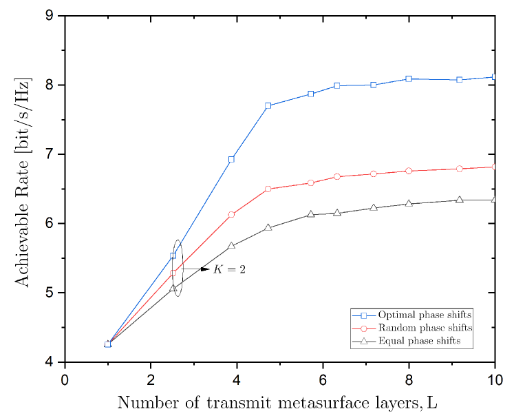
Figure 3: Achievable rate versus the number of transmit metasurfaces layers $L$ for $K=2$ layers of receive metasurfaces. Impact of phase shifts optimization of the SIMs.

In Fig. 3, we show the achievable rate versus the number of transmit metasurfaces layers $L$ for $K=2$ layers of receive metasurfaces, and we focus on the impact of optimizing the phase shifts of the SIMs. The case of optimal phase shifts achieves the best performance, while the cases random phase shifts and equal phase shifts achieve lower rate. In particular, the line, corresponding to equal phase shifts, presents the worst performance.

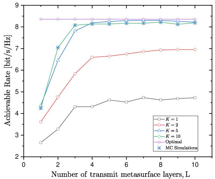
Figure 4: Achievable rate versus the number of transmit metasurfaces layers $L$ while varying the number of receiver metasurface layers $K$.

In Fig. 4, we depict the achievable rate versus the number of transmit metasurfaces layers $L$ while varying the number of receiver metasurface layers $K$. We observe that the achievable rate saturates as the number of transmit metasurface layers increases, i.e., $L\geq 3$. Also, it is shown that after a certain number of metasurfaces, the system approaches the rate obtained with only digital precoding. Digital precoding (conventional MIMO system) has been implemented for the sake of comparison. Of course, care should be taken regarding the thickness of the SIM since densely implemented metasurfaces may lead to performance loss. This can be met if their number is increased after a threshold. Notably, under these values, by increasing $L$ and $K$ after $3$ and $6$, respectively, does not improve the achievable rate.

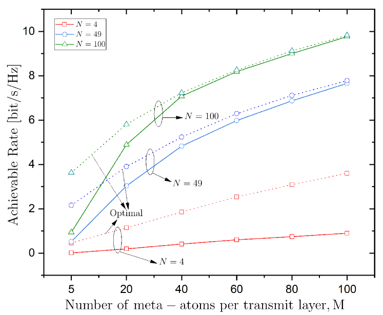
(a) Achievable rate versus the number of meta-atoms per transmit layer.

Figure 5: Impact of the numbers of meta-atoms per transmit layer and transmit antennas.

In Fig. III-B.(a), we illustrate the achievable rate versus the number of meta-atoms per transmit layer. As can be seen, the rate increases monotonically when the number of meta-atoms increase at the transmitter and receiver SIMs. Moreover, it is better to employ the receiver SIM with more meta-atoms per surface. For example, the case $M=49,N=100$ performs better than $M=100,N=49$. In Fig. III-B.(b), we show the achievable rate versus the number of transmit antennas $N_{t}$ for varying number of meta-atoms $M,N$. The rate saturates for large values of data streams due to increasing multiplexing gain. Moreover, as the number of meta-atoms increase, the rate is improved.

VI Conclusion

In this paper, we proposed a SIM-assisted HMIMO communication system, where the transmitter and the receiver are implemented by SIMs that enhance the wave-based analog precoding and combining. Specifically, we formulated the achievable rate problem, and we proposed an efficient gradient ascent algorithm that optimizes the covariance matrix of the transmitted signal and the SIM phase shifts at both sides of the transceiver simultaneously. Moreover, we obtained a Lipschitz constant guaranteeing the convergence of the proposed iterative algorithm. Numerical results confirmed that the proposed algorithm requires a lower number of iterations compared to the usually used AO approach. Finally, we showed the outperformance of the architecture with respect to its single-RIS counterpart and conventional MIMO system.

Appendix A Proof of Lemma 1

For the derivation of $\nabla_{{\mathbf{Q}}}f({\mathbf{Q}},{\bm{\phi}}_{l},{\bm{\psi}}_{k})$, we start by deriving first its differential. We have

$$d(f({\mathbf{Q}},{\bm{\phi}}_{l},{\bm{\psi}}_{k})) =\tr({\mathbf{K}}({\mathbf{Q}},{\bm{\phi}}_{l},{\bm{\psi}}_{k})d(\bar{{\mathbf{H}}}{\mathbf{Q}}\bar{{\mathbf{H}}}^{{\scriptscriptstyle\mathsf{H}}}))$$ (20bg)

$$=\tr(\bar{{\mathbf{H}}}^{{\scriptscriptstyle\mathsf{H}}}{\mathbf{K}}({\mathbf{Q}},{\bm{\phi}}_{l},{\bm{\psi}}_{k})\bar{{\mathbf{H}}}d({\mathbf{Q}})),$$ (20bh)

where, in (20bg), we have applied the property $d(\det({\mathbf{X}}))=\det({\mathbf{X}})\tr({\mathbf{X}}^{-1}d({\mathbf{X}}))$, and in (20bh), we have applied the property $\tr({\mathbf{A}}{\mathbf{B}})=\tr({\mathbf{B}}{\mathbf{A}})$. Note that we have denoted ${\mathbf{K}}({\mathbf{Q}},{\bm{\phi}}_{l},{\bm{\psi}}_{k})=\left({\bm{\mathrm{I}}}+\bar{{\mathbf{H}}}{\mathbf{Q}}\bar{{\mathbf{H}}}^{{\scriptscriptstyle\mathsf{H}}}\right)^{-1}$.

From (20bh), we obtain $\nabla_{{\mathbf{Q}}}f({\mathbf{Q}},{\bm{\phi}}_{l},{\bm{\psi}}_{k})$ by applying the suitable property from [43, Table 3.2]. Hence, we obtain

$$\nabla_{{\mathbf{Q}}}f({\mathbf{Q}},{\bm{\phi}}_{l},{\bm{\psi}}_{k}) =\frac{\partial}{{\mathbf{Q}}^{*}}f({\mathbf{Q}},{\bm{\phi}}_{l},{\bm{\psi}}_{k})$$ (20bi)

$$=\left(\frac{\partial}{{\mathbf{Q}}}f({\mathbf{Q}},{\bm{\phi}}_{l},{\bm{\psi}}_{k})\right)^{{\scriptscriptstyle\mathsf{T}}}$$ (20bj)

$$=\left(\bar{{\mathbf{H}}}^{{\scriptscriptstyle\mathsf{T}}}\left({\bm{\mathrm{I}}}+\bar{{\mathbf{H}}}^{*}{\mathbf{Q}}^{{\scriptscriptstyle\mathsf{T}}}\bar{{\mathbf{H}}}^{{\scriptscriptstyle\mathsf{T}}}\right)^{-1}\bar{{\mathbf{H}}}^{*}\right)^{{\scriptscriptstyle\mathsf{T}}}$$ (20bk)

$$=\bar{{\mathbf{H}}}^{{\scriptscriptstyle\mathsf{H}}}\left({\bm{\mathrm{I}}}+\bar{{\mathbf{H}}}{\mathbf{Q}}\bar{{\mathbf{H}}}^{{\scriptscriptstyle\mathsf{H}}}\right)^{-1}\bar{{\mathbf{H}}},$$ (20bl)

where, in the last step, we have used that ${\mathbf{Q}}^{*}={\mathbf{Q}}^{{\scriptscriptstyle\mathsf{T}}}$.

For the derivation of $\nabla_{{\bm{\phi}}_{l}}f({\mathbf{Q}},{\bm{\phi}}_{l},{\bm{\psi}}_{k})$, we focus on its differential. We have

$$d(f({\mathbf{Q}},{\bm{\phi}}_{l},{\bm{\psi}}_{k}))\!=\!\tr({\mathbf{K}}({\mathbf{Q}},{\bm{\phi}}_{l},{\bm{\psi}}_{k})(d(\bar{{\mathbf{H}}}){\mathbf{Q}}\bar{{\mathbf{H}}}^{{\scriptscriptstyle\mathsf{H}}}\!+\!\bar{{\mathbf{H}}}{\mathbf{Q}}d(\bar{{\mathbf{H}}}^{{\scriptscriptstyle\mathsf{H}}}))),$$ (20bm)

$$=\tr({\mathbf{Q}}\bar{{\mathbf{H}}}^{{\scriptscriptstyle\mathsf{H}}}{\mathbf{K}}({\mathbf{Q}},{\bm{\phi}}_{l},{\bm{\psi}}_{k})d(\bar{{\mathbf{H}}})+{\mathbf{K}}({\mathbf{Q}},{\bm{\phi}}_{l},{\bm{\psi}}_{k})\bar{{\mathbf{H}}}{\mathbf{Q}}d(\bar{{\mathbf{H}}}^{{\scriptscriptstyle\mathsf{H}}})).$$ (20bn)

From (18), it is easy to check that

$$d(\bar{{\mathbf{H}}})={\mathbf{Z}}\bar{{\mathbf{G}}}d({\mathbf{P}}),$$ (20bo)

where $\bar{{\mathbf{G}}}={\mathbf{G}}/\sqrt{N_{0}}$. Also, the differential of (10) can be written as

$$d({\mathbf{P}}) ={\bm{\Phi}}^{L}{\mathbf{W}}^{L}\cdots{\bm{\Phi}}^{l+1}{\mathbf{W}}^{l+1}d({\bm{\Phi}}^{l}){\mathbf{W}}^{l}{\bm{\Phi}}^{l-1}$$

$$\times{\mathbf{W}}^{l-1}\cdots{\bm{\Phi}}^{1}{\mathbf{W}}^{1}.$$ (20bp)

Substituting (20bp) and (20bo) into (20bn), we obtain

$$d(f({\mathbf{Q}},{\bm{\phi}}_{l},{\bm{\psi}}_{k})) =\tr({\mathbf{A}}_{l}d({\bm{\Phi}}^{l})+{\mathbf{A}}_{l}^{{\scriptscriptstyle\mathsf{H}}}d(({\bm{\Phi}}^{l})^{{\scriptscriptstyle\mathsf{H}}})),$$ (20bq)

where

$${\mathbf{A}}_{l} ={\mathbf{W}}^{l}{\bm{\Phi}}^{l-1}{\mathbf{W}}^{l-1}\cdots{\bm{\Phi}}^{1}{\mathbf{W}}^{1}{\mathbf{Q}}\bar{{\mathbf{H}}}^{{\scriptscriptstyle\mathsf{H}}}{\mathbf{K}}{\mathbf{Z}}\bar{{\mathbf{G}}}{\bm{\Phi}}^{L}$$

$$\times{\mathbf{W}}^{L}\cdots{\bm{\Phi}}^{l+1}{\mathbf{W}}^{l+1}.$$ (20br)

Now, using the property $\tr\left({\mathbf{A}}{\mathbf{B}}\right)=(\left(\text{diag}\left(\right)\left(\mathbf{A}\right)\right)^{{\scriptscriptstyle\mathsf{T}}}d(\text{diag}\left(\right)({\mathbf{B}}))$ for any matrices ${\mathbf{A}},{\mathbf{B}}$ with ${\mathbf{B}}$ being a diagonal matrix, (20bq) becomes

From (A), we can conclude that

Similar to the derivation of (A), we obtain

$$\nabla_{{\bm{\psi}}_{k}}f({\mathbf{Q}},{\bm{\phi}}_{l},{\bm{\psi}}_{k})$$

where

$${\mathbf{C}}_{k} ={\mathbf{U}}^{k}{\bm{\Psi}}^{k-1}{\mathbf{U}}^{k-1}\cdots{\bm{\Psi}}^{1}{\mathbf{U}}^{1}{\mathbf{K}}\bar{{\mathbf{H}}}{\mathbf{Q}}{\mathbf{P}}^{{\scriptscriptstyle\mathsf{H}}}\bar{{\mathbf{G}}}^{{\scriptscriptstyle\mathsf{H}}}{\bm{\Psi}}^{K}$$

$$\times{\mathbf{U}}^{K}\cdots{\bm{\Psi}}^{k+1}{\mathbf{U}}^{k+1}.$$ (20bs)

Appendix B Proof of Proposition LABEL:proposition1

During the proof, we will use the following inequalities

$$\|{\mathbf{A}}{\mathbf{B}}\| \leq\lambda_{\mathrm{max}}({\mathbf{A}})\|{\mathbf{B}}\|,$$ (20bt)

$$\|{\mathbf{A}}{\mathbf{B}}{\mathbf{C}}\| \leq\lambda_{\mathrm{max}}({\mathbf{A}})\lambda_{\mathrm{max}}({\mathbf{C}})\|{\mathbf{B}}\|,$$ (20bu)

where $\lambda_{\mathrm{max}}({\mathbf{X}})$ is the largest singular value of ${\mathbf{X}}$. Also, we have $\lambda_{\mathrm{max}}({\mathbf{Q}})\leq P$, and ${\mathbf{K}}({\mathbf{Q}},{\bm{\phi}}_{l},{\bm{\psi}}_{k})=\left({\bm{\mathrm{I}}}+\bar{{\mathbf{H}}}{\mathbf{Q}}\bar{{\mathbf{H}}}^{{\scriptscriptstyle\mathsf{H}}}\right)^{-1}\preceq{\bm{\mathrm{I}}}$, which gives

$$\lambda_{\mathrm{max}}({\mathbf{K}}({\mathbf{Q}},{\bm{\phi}}_{l},{\bm{\psi}}_{k}))\leq 1.$$ (20bv)

Making use of (LABEL:gradient1), we can write

$$\|\nabla_{{\mathbf{Q}}}f({\mathbf{Q}}^{1},{\bm{\phi}}_{l}^{1},{\bm{\psi}}_{k}^{1})-\nabla_{{\mathbf{Q}}}f({\mathbf{Q}}^{2},{\bm{\phi}}_{l}^{2},{\bm{\psi}}_{k}^{2})\|$$

$$=\|\bar{{\mathbf{H}}}_{1}^{{\scriptscriptstyle\mathsf{H}}}{\mathbf{K}}({\mathbf{Q}}^{1},{\bm{\phi}}_{l}^{1},{\bm{\psi}}_{k}^{1})\bar{{\mathbf{H}}}_{1}-\bar{{\mathbf{H}}}_{2}^{{\scriptscriptstyle\mathsf{H}}}{\mathbf{K}}({\mathbf{Q}}^{2},{\bm{\phi}}_{l}^{2},{\bm{\psi}}_{k}^{2})\bar{{\mathbf{H}}}_{2}\|$$

$$\leq\|({\mathbf{P}}^{1})^{{\scriptscriptstyle\mathsf{H}}}{\mathbf{G}}^{{\scriptscriptstyle\mathsf{H}}}({\mathbf{Z}}^{1})^{{\scriptscriptstyle\mathsf{H}}}{\mathbf{K}}({\mathbf{Q}}^{1},{\bm{\phi}}_{l}^{1},{\bm{\psi}}_{k}^{1}){\mathbf{Z}}^{1}{\mathbf{G}}{\mathbf{P}}^{1}-$$

$$({\mathbf{P}}^{1})^{{\scriptscriptstyle\mathsf{H}}}{\mathbf{G}}^{{\scriptscriptstyle\mathsf{H}}}({\mathbf{Z}}^{1})^{{\scriptscriptstyle\mathsf{H}}}{\mathbf{K}}({\mathbf{Q}}^{1},{\bm{\phi}}_{l}^{1},{\bm{\psi}}_{k}^{1}){\mathbf{Z}}^{1}{\mathbf{G}}{\mathbf{P}}^{2}\|$$

$$+\|({\mathbf{P}}^{1})^{{\scriptscriptstyle\mathsf{H}}}{\mathbf{G}}^{{\scriptscriptstyle\mathsf{H}}}({\mathbf{Z}}^{1})^{{\scriptscriptstyle\mathsf{H}}}{\mathbf{K}}({\mathbf{Q}}^{1},{\bm{\phi}}_{l}^{1},{\bm{\psi}}_{k}^{1}){\mathbf{Z}}^{1}{\mathbf{G}}{\mathbf{P}}^{2}$$

$$-({\mathbf{P}}^{2})^{{\scriptscriptstyle\mathsf{H}}}{\mathbf{G}}^{{\scriptscriptstyle\mathsf{H}}}({\mathbf{Z}}^{2})^{{\scriptscriptstyle\mathsf{H}}}{\mathbf{K}}({\mathbf{Q}}^{2},{\bm{\phi}}_{l}^{2},{\bm{\psi}}_{k}^{2}){\mathbf{Z}}^{2}{\mathbf{G}}{\mathbf{P}}^{2}\|,$$ (20bw)

where, in (20bw), we have used (18).

The first term of (20bw) can be upper-bounded as

$$\|({\mathbf{P}}^{1})^{{\scriptscriptstyle\mathsf{H}}}{\mathbf{G}}^{{\scriptscriptstyle\mathsf{H}}}({\mathbf{Z}}^{1})^{{\scriptscriptstyle\mathsf{H}}}{\mathbf{K}}({\mathbf{Q}}^{1},{\bm{\phi}}_{l}^{1},{\bm{\psi}}_{k}^{1}){\mathbf{Z}}^{1}{\mathbf{G}}{\mathbf{P}}^{1}$$

$$-({\mathbf{P}}^{1})^{{\scriptscriptstyle\mathsf{H}}}{\mathbf{G}}^{{\scriptscriptstyle\mathsf{H}}}({\mathbf{Z}}^{1})^{{\scriptscriptstyle\mathsf{H}}}{\mathbf{K}}({\mathbf{Q}}^{1},{\bm{\phi}}_{l}^{1},{\bm{\psi}}_{k}^{1}){\mathbf{Z}}^{1}{\mathbf{G}}{\mathbf{P}}^{2}\|$$

$$\leq\frac{d^{2}b^{2}f}{c^{2}}\|{\mathbf{P}}^{1}-{\mathbf{P}}^{2}\|,$$ (20bx)

where, in (20bx), we have used (LABEL:bg), (LABEL:Eqf), and (20bv).

We upper bound the second term in (20bx) as

$$\|({\mathbf{P}}^{1})^{{\scriptscriptstyle\mathsf{H}}}{\mathbf{G}}^{{\scriptscriptstyle\mathsf{H}}}({\mathbf{Z}}^{1})^{{\scriptscriptstyle\mathsf{H}}}{\mathbf{K}}({\mathbf{Q}}^{1},{\bm{\phi}}_{l}^{1},{\bm{\psi}}_{k}^{1}){\mathbf{Z}}^{1}{\mathbf{G}}{\mathbf{P}}^{2}$$

$$-({\mathbf{P}}^{2})^{{\scriptscriptstyle\mathsf{H}}}{\mathbf{G}}^{{\scriptscriptstyle\mathsf{H}}}({\mathbf{Z}}^{2})^{{\scriptscriptstyle\mathsf{H}}}{\mathbf{K}}({\mathbf{Q}}^{2},{\bm{\phi}}_{l}^{2},{\bm{\psi}}_{k}^{2}){\mathbf{Z}}^{2}{\mathbf{G}}{\mathbf{P}}^{2}\|$$

$$\leq bf\|({\mathbf{P}}^{1})^{{\scriptscriptstyle\mathsf{H}}}{\mathbf{G}}^{{\scriptscriptstyle\mathsf{H}}}({\mathbf{Z}}^{1})^{{\scriptscriptstyle\mathsf{H}}}{\mathbf{K}}({\mathbf{Q}}^{1},{\bm{\phi}}_{l}^{1},{\bm{\psi}}_{k}^{1}){\mathbf{Z}}^{1}$$

$$-({\mathbf{P}}^{2})^{{\scriptscriptstyle\mathsf{H}}}{\mathbf{G}}^{{\scriptscriptstyle\mathsf{H}}}({\mathbf{Z}}^{2})^{{\scriptscriptstyle\mathsf{H}}}{\mathbf{K}}({\mathbf{Q}}^{2},{\bm{\phi}}_{l}^{2},{\bm{\psi}}_{k}^{2}){\mathbf{Z}}^{2}\|$$ (20by)

$$\leq bf\big{(}\|({\mathbf{P}}^{1})^{{\scriptscriptstyle\mathsf{H}}}{\mathbf{G}}^{{\scriptscriptstyle\mathsf{H}}}({\mathbf{Z}}^{1})^{{\scriptscriptstyle\mathsf{H}}}{\mathbf{K}}({\mathbf{Q}}^{1},{\bm{\phi}}_{l}^{1},{\bm{\psi}}_{k}^{1}){\mathbf{Z}}^{1}$$

$$-({\mathbf{P}}^{2})^{{\scriptscriptstyle\mathsf{H}}}{\mathbf{G}}^{{\scriptscriptstyle\mathsf{H}}}({\mathbf{Z}}^{1})^{{\scriptscriptstyle\mathsf{H}}}{\mathbf{K}}({\mathbf{Q}}^{1},{\bm{\phi}}_{l}^{1},{\bm{\psi}}_{k}^{1}){\mathbf{Z}}^{1}\|$$

$$+\|({\mathbf{P}}^{2})^{{\scriptscriptstyle\mathsf{H}}}{\mathbf{G}}^{{\scriptscriptstyle\mathsf{H}}}({\mathbf{Z}}^{1})^{{\scriptscriptstyle\mathsf{H}}}{\mathbf{K}}({\mathbf{Q}}^{1},{\bm{\phi}}_{l}^{1},{\bm{\psi}}_{k}^{1}){\mathbf{Z}}^{1}$$

$$-({\mathbf{P}}^{2})^{{\scriptscriptstyle\mathsf{H}}}{\mathbf{G}}^{{\scriptscriptstyle\mathsf{H}}}({\mathbf{Z}}^{2})^{{\scriptscriptstyle\mathsf{H}}}{\mathbf{K}}({\mathbf{Q}}^{2},{\bm{\phi}}_{l}^{2},{\bm{\psi}}_{k}^{2}){\mathbf{Z}}^{2}\|\big{)},$$ (20bz)

where, in (20by), we have used (LABEL:bg) and (LABEL:Eqd).

The first term of (20bz) results in

$$\!\!\!\|({\mathbf{P}}^{1})^{{\scriptscriptstyle\mathsf{H}}}{\mathbf{G}}^{{\scriptscriptstyle\mathsf{H}}}({\mathbf{Z}}^{1})^{{\scriptscriptstyle\mathsf{H}}}{\mathbf{K}}({\mathbf{Q}}^{1},{\bm{\phi}}_{l}^{1},{\bm{\psi}}_{k}^{1}){\mathbf{Z}}^{1}$$

$$\!\!-({\mathbf{P}}^{2})^{{\scriptscriptstyle\mathsf{H}}}{\mathbf{G}}^{{\scriptscriptstyle\mathsf{H}}}({\mathbf{Z}}^{1})^{{\scriptscriptstyle\mathsf{H}}}{\mathbf{K}}({\mathbf{Q}}^{1},{\bm{\phi}}_{l}^{1},{\bm{\psi}}_{k}^{1}){\mathbf{Z}}^{1}\|\leq\frac{bd^{2}}{c^{2}}\|{\mathbf{P}}^{1}-{\mathbf{P}}^{2}\|,$$ (20ca)

where we have used (20bv).

The second term in (20bz) becomes

$$\|({\mathbf{P}}^{2})^{{\scriptscriptstyle\mathsf{H}}}{\mathbf{G}}^{{\scriptscriptstyle\mathsf{H}}}({\mathbf{Z}}^{1})^{{\scriptscriptstyle\mathsf{H}}}{\mathbf{K}}({\mathbf{Q}}^{1},{\bm{\phi}}_{l}^{1},{\bm{\psi}}_{k}^{1}){\mathbf{Z}}^{1}$$

$$-({\mathbf{P}}^{2})^{{\scriptscriptstyle\mathsf{H}}}{\mathbf{G}}^{{\scriptscriptstyle\mathsf{H}}}({\mathbf{Z}}^{2})^{{\scriptscriptstyle\mathsf{H}}}{\mathbf{K}}({\mathbf{Q}}^{2},{\bm{\phi}}_{l}^{2},{\bm{\psi}}_{k}^{2}){\mathbf{Z}}^{2}\|$$

$$\leq bf\|({\mathbf{Z}}^{1})^{{\scriptscriptstyle\mathsf{H}}}{\mathbf{K}}({\mathbf{Q}}^{1},{\bm{\phi}}_{l}^{1},{\bm{\psi}}_{k}^{1}){\mathbf{Z}}^{1}-({\mathbf{Z}}^{2})^{{\scriptscriptstyle\mathsf{H}}}{\mathbf{K}}({\mathbf{Q}}^{2},{\bm{\phi}}_{l}^{2},{\bm{\psi}}_{k}^{2}){\mathbf{Z}}^{2}\|$$ (20cb)

$$\leq bf\big{(}\|({\mathbf{Z}}^{1})^{{\scriptscriptstyle\mathsf{H}}}{\mathbf{K}}({\mathbf{Q}}^{1},{\bm{\phi}}_{l}^{1},{\bm{\psi}}_{k}^{1}){\mathbf{Z}}^{1}-({\mathbf{Z}}^{2})^{{\scriptscriptstyle\mathsf{H}}}{\mathbf{K}}({\mathbf{Q}}^{1},{\bm{\phi}}_{l}^{1},{\bm{\psi}}_{k}^{1}){\mathbf{Z}}^{1}\|$$

$$+\|({\mathbf{Z}}^{2})^{{\scriptscriptstyle\mathsf{H}}}{\mathbf{K}}({\mathbf{Q}}^{1},{\bm{\phi}}_{l}^{1},{\bm{\psi}}_{k}^{1}){\mathbf{Z}}^{1}-({\mathbf{Z}}^{2})^{{\scriptscriptstyle\mathsf{H}}}{\mathbf{K}}({\mathbf{Q}}^{2},{\bm{\phi}}_{l}^{2},{\bm{\psi}}_{k}^{2}){\mathbf{Z}}^{2}\|\big{)}$$ (20cc)

$$\leq\frac{2bfd}{c}\big{(}\|{\mathbf{Z}}^{1}-{\mathbf{Z}}^{2}\|,$$ (20cd)

where, in (20cb), we have used (LABEL:bg) and (20bv).

Substitution of (20ca) and (20cd) into (20by) gives

$$\|({\mathbf{P}}^{1})^{{\scriptscriptstyle\mathsf{H}}}{\mathbf{G}}^{{\scriptscriptstyle\mathsf{H}}}({\mathbf{Z}}^{1})^{{\scriptscriptstyle\mathsf{H}}}{\mathbf{K}}({\mathbf{Q}}^{1},{\bm{\phi}}_{l}^{1},{\bm{\psi}}_{k}^{1}){\mathbf{Z}}^{1}{\mathbf{G}}{\mathbf{P}}^{2}$$

$$-({\mathbf{P}}^{2})^{{\scriptscriptstyle\mathsf{H}}}{\mathbf{G}}^{{\scriptscriptstyle\mathsf{H}}}({\mathbf{Z}}^{2})^{{\scriptscriptstyle\mathsf{H}}}{\mathbf{K}}({\mathbf{Q}}^{2},{\bm{\phi}}_{l}^{2},{\bm{\psi}}_{k}^{2}){\mathbf{Z}}^{2}{\mathbf{G}}{\mathbf{P}}^{2}\|$$

$$\leq bf\big{(}\frac{bd^{2}}{c^{2}}\|{\mathbf{P}}^{1}-{\mathbf{P}}^{2}\|+\frac{2bfd}{c}\big{(}\|{\mathbf{Z}}^{1}-{\mathbf{Z}}^{2}\|\big{)}.$$ (20ce)

Now, inserting (20bx) and (20ce) into (20bw), we obtain

$$\|\nabla_{{\mathbf{Q}}}f({\mathbf{Q}}^{1},{\bm{\phi}}_{l}^{1},{\bm{\psi}}_{k}^{1})-\nabla_{{\mathbf{Q}}}f({\mathbf{Q}}^{2},{\bm{\phi}}_{l}^{2},{\bm{\psi}}_{k}^{2})\|$$

$$\leq bf\big{(}\frac{2bd^{2}}{c^{2}}\|{\mathbf{P}}^{1}-{\mathbf{P}}^{2}\|+\frac{2bfd}{c}\big{(}\|{\mathbf{Z}}^{1}-{\mathbf{Z}}^{2}\|\big{)}.$$ (20cf)

Using (LABEL:gradient2), we obtain

$$\|\nabla_{{\bm{\phi}}_{l}}f({\mathbf{Q}}^{1},{\bm{\phi}}_{l}^{1},{\bm{\psi}}_{k}^{1})-\nabla_{{\bm{\phi}}_{l}}f({\mathbf{Q}}^{2},{\bm{\phi}}_{l}^{2},{\bm{\psi}}_{k}^{2})$$

$$\|\leq\|{\mathbf{K}}({\mathbf{Q}}^{1},{\bm{\phi}}_{l}^{1},{\bm{\psi}}_{k}^{1}){\mathbf{A}}_{l,1}^{{\scriptscriptstyle\mathsf{H}}}-{\mathbf{K}}({\mathbf{Q}}^{2},{\bm{\phi}}_{l}^{2},{\bm{\psi}}_{k}^{2}){\mathbf{A}}_{l,2}^{{\scriptscriptstyle\mathsf{H}}}\|$$ (20cg)

$$\leq a_{l}b\|{\mathbf{Q}}^{1}\bar{{\mathbf{H}}}_{1}^{{\scriptscriptstyle\mathsf{H}}}{\mathbf{Z}}^{1}-{\mathbf{Q}}^{2}\bar{{\mathbf{H}}}_{2}^{{\scriptscriptstyle\mathsf{H}}}{\mathbf{Z}}^{2}\|$$ (20ch)

$$=a_{l}b\|{\mathbf{Q}}^{1}\bar{{\mathbf{H}}}_{1}^{{\scriptscriptstyle\mathsf{H}}}{\mathbf{Z}}^{1}-{\mathbf{Q}}^{2}\bar{{\mathbf{H}}}_{1}^{{\scriptscriptstyle\mathsf{H}}}{\mathbf{Z}}^{1}+{\mathbf{Q}}^{2}\bar{{\mathbf{H}}}_{1}^{{\scriptscriptstyle\mathsf{H}}}{\mathbf{Z}}^{1}-{\mathbf{Q}}^{2}\bar{{\mathbf{H}}}_{2}^{{\scriptscriptstyle\mathsf{H}}}{\mathbf{Z}}^{2}\|$$ (20ci)

$$\leq a_{l}b\big{(}\|{\mathbf{Q}}^{1}\bar{{\mathbf{H}}}_{1}^{{\scriptscriptstyle\mathsf{H}}}{\mathbf{Z}}^{1}-{\mathbf{Q}}^{2}\bar{{\mathbf{H}}}_{1}^{{\scriptscriptstyle\mathsf{H}}}{\mathbf{Z}}^{1}\|+\|{\mathbf{Q}}^{2}\bar{{\mathbf{H}}}_{1}^{{\scriptscriptstyle\mathsf{H}}}{\mathbf{Z}}^{1}-{\mathbf{Q}}^{2}\bar{{\mathbf{H}}}_{2}^{{\scriptscriptstyle\mathsf{H}}}{\mathbf{Z}}^{2}\|\big{)},$$ (20cj)

where, in (20cg), we have used that $\|\text{diag}\left(\right)({\mathbf{X}})\|\leq\|{\mathbf{X}}\|$. In (20ch), we have used (20bv), (LABEL:al), and (LABEL:bg).

We upper-bound the first term on the right-hand side of (20cj) as

$$\|{\mathbf{Q}}^{1}\bar{{\mathbf{H}}}_{1}^{{\scriptscriptstyle\mathsf{H}}}{\mathbf{Z}}^{1}-{\mathbf{Q}}^{2}\bar{{\mathbf{H}}}_{1}^{{\scriptscriptstyle\mathsf{H}}}{\mathbf{Z}}^{1}\|\leq c\|{\mathbf{Q}}^{1}-{\mathbf{Q}}^{2}\|,$$ (20ck)

where we have used (LABEL:Eqd).

The second term of (20cj) can be written

$$\|{\mathbf{Q}}^{2}\bar{{\mathbf{H}}}_{1}^{{\scriptscriptstyle\mathsf{H}}}{\mathbf{Z}}^{1}-{\mathbf{Q}}^{2}\bar{{\mathbf{H}}}_{2}^{{\scriptscriptstyle\mathsf{H}}}{\mathbf{Z}}^{2}\|\leq P\|\bar{{\mathbf{H}}}_{1}^{{\scriptscriptstyle\mathsf{H}}}{\mathbf{Z}}^{1}-\bar{{\mathbf{H}}}_{2}^{{\scriptscriptstyle\mathsf{H}}}{\mathbf{Z}}^{2}\|$$ (20cl)

$$=P\|\bar{{\mathbf{H}}}_{1}^{{\scriptscriptstyle\mathsf{H}}}{\mathbf{Z}}^{1}-\bar{{\mathbf{H}}}_{1}^{{\scriptscriptstyle\mathsf{H}}}{\mathbf{Z}}^{2}+\bar{{\mathbf{H}}}_{1}^{{\scriptscriptstyle\mathsf{H}}}{\mathbf{Z}}^{2}-\bar{{\mathbf{H}}}_{2}^{{\scriptscriptstyle\mathsf{H}}}{\mathbf{Z}}^{2}\|$$ (20cm)

$$\leq P\big{(}\|\bar{{\mathbf{H}}}_{1}^{{\scriptscriptstyle\mathsf{H}}}{\mathbf{Z}}^{1}-\bar{{\mathbf{H}}}_{1}^{{\scriptscriptstyle\mathsf{H}}}{\mathbf{Z}}^{2}\|+\|\bar{{\mathbf{H}}}_{1}^{{\scriptscriptstyle\mathsf{H}}}{\mathbf{Z}}^{2}-\bar{{\mathbf{H}}}_{2}^{{\scriptscriptstyle\mathsf{H}}}{\mathbf{Z}}^{2}\|\big{)}.$$ (20cn)

The first term in (20cn) can be written as

$$\|\bar{{\mathbf{H}}}_{1}^{{\scriptscriptstyle\mathsf{H}}}{\mathbf{Z}}^{1}-\bar{{\mathbf{H}}}_{1}^{{\scriptscriptstyle\mathsf{H}}}{\mathbf{Z}}^{2}\|\leq c\|{\mathbf{Z}}^{1}-{\mathbf{Z}}^{2}\|,$$ (20co)

where we have used (LABEL:Eqc).

Next, the second term in (20cn) becomes

$$\|\bar{{\mathbf{H}}}_{1}^{{\scriptscriptstyle\mathsf{H}}}{\mathbf{Z}}^{2}-\bar{{\mathbf{H}}}_{2}^{{\scriptscriptstyle\mathsf{H}}}{\mathbf{Z}}^{2}\|\leq\frac{d}{c}\|\bar{{\mathbf{H}}}_{1}-\bar{{\mathbf{H}}}_{2}\|$$ (20cp)

$$=\frac{d}{cN_{0}}\|{\mathbf{Z}}^{1}{\mathbf{G}}{\mathbf{P}}^{1}-{\mathbf{Z}}^{2}{\mathbf{G}}{\mathbf{P}}^{2}\|$$ (20cq)

$$=\frac{d}{cN_{0}}\|{\mathbf{Z}}^{1}{\mathbf{G}}{\mathbf{P}}^{1}-{\mathbf{Z}}^{2}{\mathbf{G}}{\mathbf{P}}^{1}+{\mathbf{Z}}^{2}{\mathbf{G}}{\mathbf{P}}^{1}-{\mathbf{Z}}^{2}{\mathbf{G}}{\mathbf{P}}^{2}\|$$ (20cr)

$$=\frac{d}{cN_{0}}\big{(}\|{\mathbf{Z}}^{1}{\mathbf{G}}{\mathbf{P}}^{1}-{\mathbf{Z}}^{2}{\mathbf{G}}{\mathbf{P}}^{1}\|+\|{\mathbf{Z}}^{2}{\mathbf{G}}{\mathbf{P}}^{1}-{\mathbf{Z}}^{2}{\mathbf{G}}{\mathbf{P}}^{2}\|\big{)},$$ (20cs)

where, in (20cp), we have used (LABEL:Eqd). In (20cq), we have inserted (18).

The first term in (20cs) becomes

$$\|{\mathbf{Z}}^{1}{\mathbf{G}}{\mathbf{P}}^{1}-{\mathbf{Z}}^{2}{\mathbf{G}}{\mathbf{P}}^{1}\|\leq bf\|{\mathbf{Z}}^{1}-{\mathbf{Z}}^{2}\|$$ (20ct)

where we have used (LABEL:Eqf). The second term in (20cs) yields

$$\|{\mathbf{Z}}^{2}{\mathbf{G}}{\mathbf{P}}^{1}-{\mathbf{Z}}^{2}{\mathbf{G}}{\mathbf{P}}^{2}\|\leq b\frac{d}{c}\|{\mathbf{P}}^{1}-{\mathbf{P}}^{2}\|.$$ (20cu)

By substituting (20ct) and (20cu) into (20cs), we obtain

$$\|\bar{{\mathbf{H}}}_{1}^{{\scriptscriptstyle\mathsf{H}}}{\mathbf{Z}}^{2}-\bar{{\mathbf{H}}}_{2}^{{\scriptscriptstyle\mathsf{H}}}{\mathbf{Z}}^{2}\| \leq\frac{bd}{cN_{0}}\big{(}f\|{\mathbf{Z}}^{1}-{\mathbf{Z}}^{2}\|+\frac{d}{c}\|{\mathbf{P}}^{1}-{\mathbf{P}}^{2}\|\big{)}.$$ (20cv)

Inserting (20co) and (20cv) into (20cn)

$$\|{\mathbf{Q}}^{2}\bar{{\mathbf{H}}}_{1}^{{\scriptscriptstyle\mathsf{H}}}{\mathbf{Z}}^{1}-{\mathbf{Q}}^{2}\bar{{\mathbf{H}}}_{2}^{{\scriptscriptstyle\mathsf{H}}}{\mathbf{Z}}^{2}\| \leq P\left(c+\frac{bdf}{cN_{0}}\right)\|{\mathbf{Z}}^{1}-{\mathbf{Z}}^{2}\|$$

$$+P\frac{bd^{2}}{c^{2}N_{0}}\|{\mathbf{P}}^{1}-{\mathbf{P}}^{2}\|.$$ (20cw)

Finally, substituting (20cw) and (20ck) into (20cj), we derive

$$\|\nabla_{{\bm{\phi}}_{l}}f({\mathbf{Q}}^{1},{\bm{\phi}}_{l}^{1},{\bm{\psi}}_{k}^{1})-\nabla_{{\bm{\phi}}_{l}}f({\mathbf{Q}}^{2},{\bm{\phi}}_{l}^{2},{\bm{\psi}}_{k}^{2})\|\leq a_{l}bc|{\mathbf{Q}}^{1}-{\mathbf{Q}}^{2}\|$$

$$+a_{l}bP\left(c+\frac{bdf}{cN_{0}}\right)\|{\mathbf{Z}}^{1}-{\mathbf{Z}}^{2}\|$$

$$+a_{l}P\frac{b^{2}d^{2}}{c^{2}N_{0}}\|{\mathbf{P}}^{1}-{\mathbf{P}}^{2}\|.$$ (20cx)

The inequality regarding $\nabla_{{\bm{\psi}}_{k}}f({\mathbf{Q}},{\bm{\phi}}_{l},{\bm{\psi}}_{k})$ can be written as

$$\|\nabla_{{\bm{\psi}}_{k}}f({\mathbf{Q}}^{1},{\bm{\phi}}_{l}^{1},{\bm{\psi}}_{k}^{1})-\nabla_{{\bm{\psi}}_{k}}f({\mathbf{Q}}^{2},{\bm{\phi}}_{l}^{2},{\bm{\psi}}_{k}^{2})\|$$

$$\leq\|{\mathbf{K}}({\mathbf{Q}}^{1},{\bm{\phi}}_{l}^{1},{\bm{\psi}}_{k}^{1}){\mathbf{C}}_{k,1}^{{\scriptscriptstyle\mathsf{H}}}-{\mathbf{K}}({\mathbf{Q}}^{2},{\bm{\phi}}_{l}^{2},{\bm{\psi}}_{k}^{2}{\mathbf{C}}_{k,2}^{{\scriptscriptstyle\mathsf{H}}})\|.$$ (20cy)

In a similar way, we can upper bound the previous inequality. We omit the details due to limited space. Hence, we conclude the proof.

Appendix C Proof of Theorem LABEL:Theorem1

According to Lemma (1), we can write

$$\|\nabla_{{\mathbf{Q}}}f({\mathbf{Q}}^{1},{\bm{\phi}}_{l}^{1},{\bm{\psi}}_{k}^{1})-\nabla_{{\mathbf{Q}}}f({\mathbf{Q}}^{2},{\bm{\phi}}_{l}^{2},{\bm{\psi}}_{k}^{2})\|^{2}$$

$$+\|\nabla_{{\bm{\phi}}_{l}}f({\mathbf{Q}}^{1},{\bm{\phi}}_{l}^{1},{\bm{\psi}}_{k}^{1})-\nabla_{{\bm{\phi}}_{l}}f({\mathbf{Q}}^{2},{\bm{\phi}}_{l}^{2},{\bm{\psi}}_{k}^{2})\|^{2}$$

$$+\|\nabla_{{\bm{\psi}}_{k}}f({\mathbf{Q}}^{1},{\bm{\phi}}_{l}^{1},{\bm{\psi}}_{k}^{1})-\nabla_{{\bm{\psi}}_{k}}f({\mathbf{Q}}^{2},{\bm{\phi}}_{l}^{2},{\bm{\psi}}_{k}^{2})\|$$

$$\leq\Lambda_{{\mathbf{Q}}}^{2}\|{\mathbf{Q}}^{1}-{\mathbf{Q}}^{2}\|^{2}+\Lambda_{{\bm{\phi}}_{l}}^{2}\|{\mathbf{P}}^{1}-{\mathbf{P}}^{2}\|^{2}+\Lambda_{{\bm{\psi}}_{k}}^{2}\|{\mathbf{Z}}^{1}-{\mathbf{Z}}^{2}\|^{2}$$

$$\leq\max(\Lambda_{{\mathbf{Q}}}^{2},\Lambda_{{\bm{\phi}}_{l}}^{2},\Lambda_{{\bm{\psi}}_{k}}^{2})\big{(}\|{\mathbf{Q}}^{1}-{\mathbf{Q}}^{2}\|^{2}+\|{\mathbf{P}}^{1}-{\mathbf{P}}^{2}\|^{2}$$

$$+\|{\mathbf{Z}}^{1}-{\mathbf{Z}}^{2}\|^{2}\big{)}.$$ (20cz)

Applying the square root on both sides of (20cz) together with the inequality

$$2\|{\mathbf{Q}}^{1}-{\mathbf{Q}}^{2}\|\cdot\|{\mathbf{P}}^{1}-{\mathbf{P}}^{2}\|+2\|{\mathbf{Z}}^{1}-{\mathbf{Z}}^{2}\|\cdot\|{\mathbf{P}}^{1}-{\mathbf{P}}^{2}\|$$

$$+2\|{\mathbf{Q}}^{1}-{\mathbf{Q}}^{2}\|\cdot\|{\mathbf{Z}}^{1}-{\mathbf{Z}}^{2}\|$$

$$\leq\|{\mathbf{Q}}^{1}-{\mathbf{Q}}^{2}\|^{2}+\|{\mathbf{P}}^{1}-{\mathbf{P}}^{2}\|+\|{\mathbf{Z}}^{1}-{\mathbf{Z}}^{2}\|,$$ (20da)

we observe that $\max(\Lambda_{{\mathbf{Q}}}^{2},\Lambda_{{\bm{\phi}}_{l}}^{2},\Lambda_{{\bm{\psi}}_{k}}^{2})$ is a Lipschitz constant of the gradient of $f({\mathbf{Q}},{\bm{\phi}}_{l},{\bm{\psi}}_{k})$, which concludes the proof.

Appendix D Proof of Theorem LABEL:Theorem2

The point ${\mathbf{Q}}^{n+1}$ can be projected onto $\mathcal{Q}$ according to the following equation.

$${\mathbf{Q}}^{n+1} =\arg\min_{{\mathbf{Q}}\in\mathcal{Q}}\|{\mathbf{Q}}-{\mathbf{Q}}^{n}-\mu_{n}^{1}\nabla_{\mathcal{Q}}f({\mathbf{Q}}^{n},{\bm{\phi}}_{l}^{n},{\bm{\psi}}_{k}^{n})\|^{2}$$

$$=\arg\max_{{\mathbf{Q}}\in\mathcal{Q}}\langle\nabla_{\mathcal{Q}}f({\mathbf{Q}}^{n},{\bm{\phi}}_{l}^{n},{\bm{\psi}}_{k}^{n}),{\mathbf{Q}}-{\mathbf{Q}}^{n}\rangle$$

$$-\frac{1}{2\mu_{n}^{1}}\|{\mathbf{Q}}-{\mathbf{Q}}^{n}\|^{2}.$$ (20db)

In the case of ${\mathbf{Q}}-{\mathbf{Q}}^{n}$, we meet that the objective is $0$, which means that

$$\!\!\!\!\!\langle\nabla_{\mathcal{Q}}f({\mathbf{Q}}^{n},{\bm{\phi}}_{l}^{n},{\bm{\psi}}_{k}^{n}),{\mathbf{Q}}-{\mathbf{Q}}^{n}\rangle-\frac{1}{2\mu_{n}^{1}}\|{\mathbf{Q}}-{\mathbf{Q}}^{n}\|^{2}\geq 0.$$ (20dc)

Similarly, we obtain

$$\langle\nabla_{{\bm{\phi}}_{l}}f({\mathbf{Q}}^{n},{\bm{\phi}}_{l}^{n},{\bm{\psi}}_{k}^{n}),{\bm{\phi}}_{l}-{\bm{\phi}}_{l}^{n}\rangle-\frac{1}{2\mu_{n}^{2}}\|{\bm{\phi}}_{l}-{\bm{\phi}}_{l}^{n}\|^{2}\geq 0,$$ (20dd)

$$\langle\nabla_{{\bm{\psi}}_{k}}f({\mathbf{Q}}^{n},{\bm{\phi}}_{l}^{n},{\bm{\psi}}_{k}^{n}),{\bm{\psi}}_{k}-{\bm{\psi}}_{k}^{n}\rangle-\frac{1}{2\mu_{n}^{3}}\|{\bm{\psi}}_{k}-{\bm{\psi}}_{k}^{n}\|^{2}\geq 0.$$ (20de)

Now, applying the following inequality

$$f({\mathbf{y}})\geq f({\mathbf{y}})+\langle\nabla f({\mathbf{x}}),{\mathbf{y}}-{\mathbf{x}}\rangle-\frac{\Lambda}{2}\|{\mathbf{y}}-{\mathbf{x}}\|^{2},$$ (20df)

which holds for any $\Lambda$-smooth function $f({\mathbf{x}})$, we obtain

$$f({\mathbf{Q}}^{n+1},{\bm{\phi}}_{l}^{n+1},{\bm{\psi}}_{k}^{n+1})\geq f({\mathbf{Q}}^{n},{\bm{\phi}}_{l}^{n},{\bm{\psi}}_{k}^{n})$$

$$+\langle\nabla_{\mathcal{Q}}f({\mathbf{Q}}^{n},{\bm{\phi}}_{l}^{n},{\bm{\psi}}_{k}^{n}),{\mathbf{Q}}-{\mathbf{Q}}^{n}\rangle$$

$$+\langle\nabla_{{\bm{\phi}}_{l}}f({\mathbf{Q}}^{n},{\bm{\phi}}_{l}^{n},{\bm{\psi}}_{k}^{n}),{\bm{\phi}}_{l}-{\bm{\phi}}_{l}^{n}\rangle$$

$$+\langle\nabla_{{\bm{\psi}}_{k}}f({\mathbf{Q}}^{n},{\bm{\phi}}_{l}^{n},{\bm{\psi}}_{k}^{n}),{\bm{\psi}}_{k}-{\bm{\psi}}_{k}^{n}\rangle$$

$$-\frac{\Lambda}{2}\|{\mathbf{Q}}^{n+1}-{\mathbf{Q}}^{n}\|^{2}-\frac{\Lambda}{2}\|{\bm{\phi}}_{l}^{n+1}-{\bm{\phi}}_{l}^{n}\|^{2}-\frac{\Lambda}{2}\|{\bm{\psi}}_{k}^{n+1}-{\bm{\psi}}_{k}^{n}\|^{2}$$

$$\geq f({\mathbf{Q}}^{n},{\bm{\phi}}_{l}^{n},{\bm{\psi}}_{k}^{n})+\left(\frac{1}{2\mu_{n}^{1}}-\frac{\Lambda}{2}\right)\|{\mathbf{Q}}^{n+1}-{\mathbf{Q}}^{n}\|^{2}$$

$$+\left(\frac{1}{2\mu_{n}^{2}}-\frac{\Lambda}{2}\right)\|{\bm{\phi}}_{l}^{n+1}-{\bm{\phi}}_{l}^{n}\|^{2}$$

$$+\left(\frac{1}{2\mu_{n}^{3}}-\frac{\Lambda}{2}\right)\|{\bm{\psi}}_{k}^{n+1}-{\bm{\psi}}_{k}^{n}\|^{2},$$ (20dg)

where, in the first inequality, we have applied Theorem 1.

From the above equation, when $\mu_{n}^{q}<\frac{1}{\Lambda}$ for $q=1,2,3$, we observe that $f({\mathbf{Q}}^{n+1},{\bm{\phi}}_{l}^{n+1},{\bm{\psi}}_{k}^{n+1})\geq f({\mathbf{Q}}^{n},{\bm{\phi}}_{l}^{n},{\bm{\psi}}_{k}^{n})$. Now, we denote $f^{\star}$ the value of $f$ at all accumulation points, and we write (20dg) as

$$f({\mathbf{Q}}^{n+1},{\bm{\phi}}_{l}^{n+1},{\bm{\psi}}_{k}^{n+1})-f({\mathbf{Q}}^{n},{\bm{\phi}}_{l}^{n},{\bm{\psi}}_{k}^{n})\geq\left(\frac{1}{2\mu_{n}^{1}}-\frac{\Lambda}{2}\right)$$

$$\times\|{\mathbf{Q}}^{n+1}-{\mathbf{Q}}^{n}\|^{2}+\left(\frac{1}{2\mu_{n}^{2}}-\frac{\Lambda}{2}\right)\|{\bm{\phi}}_{l}^{n+1}-{\bm{\phi}}_{l}^{n}\|^{2}$$

$$+\left(\frac{1}{2\mu_{n}^{3}}-\frac{\Lambda}{2}\right)\|{\bm{\psi}}_{k}^{n+1}-{\bm{\psi}}_{k}^{n}\|^{2},$$ (20dh)

which gives

$$\infty>f^{\star}-f({\mathbf{Q}}^{1},{\bm{\phi}}_{l}^{1},{\bm{\psi}}_{k}^{1})>\sum_{n=1}^{\infty}\Bigg{(}\left(\frac{1}{2\mu_{n}^{1}}-\frac{\Lambda}{2}\right)$$

$$\times\|{\mathbf{Q}}^{n+1}-{\mathbf{Q}}^{n}\|^{2}+\left(\frac{1}{2\mu_{n}^{2}}-\frac{\Lambda}{2}\right)\|{\bm{\phi}}_{l}^{n+1}-{\bm{\phi}}_{l}^{n}\|^{2}$$

$$+\left(\frac{1}{2\mu_{n}^{3}}-\frac{\Lambda}{2}\right)\|{\bm{\psi}}_{k}^{n+1}-{\bm{\psi}}_{k}^{n}\|^{2}\Bigg{)}.$$ (20di)

Given that $\mu_{n}^{q}<\frac{1}{\Lambda}$ for $q=1,2,3$, we result in

$$\|{\mathbf{Q}}^{n+1}-{\mathbf{Q}}^{n}\| \to 0,$$ (20dj)

$$\|{\bm{\phi}}_{l}^{n+1}-{\bm{\phi}}_{l}^{n}\| \to 0,$$ (20dk)

$$\|{\bm{\psi}}_{k}^{n+1}-{\bm{\psi}}_{k}^{n}\| \to 0.$$ (20dl)

The condition in (20db), concerning optimality, can be written as

$$\langle\frac{1}{\mu_{n}^{i}}\left({\mathbf{Q}}^{n+1}-{\mathbf{Q}}^{n}\right)-\nabla_{\mathcal{Q}}f({\mathbf{Q}}^{n},{\bm{\phi}}_{l}^{n},{\bm{\psi}}_{k}^{n}),{\mathbf{Q}}-{\mathbf{Q}}^{n+1}\rangle$$

$$\leq 0,\forall{\mathbf{Q}}\in\mathcal{Q}.$$ (20dm)

Similar inequalities hold for the other two parameters ${\bm{\phi}}_{l}$ and ${\bm{\psi}}_{k}$.

By setting $n\to\infty$ in (20dm), we obtain

$$\langle-\nabla_{\mathcal{Q}}f({\mathbf{Q}}^{*},{\bm{\phi}}_{l}^{*},{\bm{\psi}}_{k}^{*}),{\mathbf{Q}}-{\mathbf{Q}}^{\star}\rangle\leq 0,\forall{\mathbf{Q}}\in\mathcal{Q}$$ (20dn)

due to the continuity of the gradient of $f({\mathbf{Q}}^{n},{\bm{\phi}}_{l}^{n},{\bm{\psi}}_{k}^{n})$, i.e., $\nabla_{\mathcal{Q}}f({\mathbf{Q}}^{n},{\bm{\phi}}_{l}^{n},{\bm{\psi}}_{k}^{n})\to\nabla_{\mathcal{Q}}f({\mathbf{Q}}^{*},{\bm{\phi}}_{l}^{*},{\bm{\psi}}_{k}^{*})$.

In the case of ${\bm{\phi}}_{l}$ and ${\bm{\psi}}_{k}$, similar observations hold, which signifies that $({\mathbf{Q}}^{*},{\bm{\phi}}_{l}^{*},{\bm{\psi}}_{k}^{*})$ is a critical point of Problem $(\mathcal{P})$, and this concludes the proof.

solutionfile

References

• [1] K. B. Letaief et al., “The roadmap to 6G: AI empowered wireless networks,” IEEE Commun. Mag., vol. 57, no. 8, pp. 84–90, 2019.
• [2] S. Dang et al., “What should 6G be?” Nature Electronics, vol. 3, no. 1, pp. 20–29, 2020.
• [3] J. G. Andrews et al., “What will 5G be?” IEEE J. Sel. Areas Commun., vol. 32, no. 6, pp. 1065–1082, 2014.
• [4] M. Di Renzo et al., “Smart radio environments empowered by reconfigurable intelligent surfaces: How it works, state of research, and the road ahead,” IEEE J. Sel. Areas Commun., vol. 38, no. 11, pp. 2450–2525, 2020.
• [5] Q. Wu and R. Zhang, “Towards smart and reconfigurable environment: Intelligent reflecting surface aided wireless network,” IEEE Commun. Mag., vol. 58, no. 1, pp. 106–112.
• [6] A. Papazafeiropoulos et al., “Intelligent reflecting surface-assisted MU-MISO systems with imperfect hardware: Channel estimation and beamforming design,” IEEE Trans. Wireless Commun., vol. 21, no. 3, pp. 2077–2092, 2021.
• [7] ——, “Cooperative RIS and STAR-RIS assisted mMIMO communication: Analysis and optimization,” vol. 72, no. 9, pp. 11 975–11 989.
• [8] C. Huang et al., “Holographic MIMO surfaces for 6G wireless networks: Opportunities, challenges, and trends,” IEEE Wireless Commun., vol. 27, no. 5, pp. 118–125, 2020.
• [9] Q. Wu and R. Zhang, “Intelligent reflecting surface enhanced wireless network via joint active and passive beamforming,” IEEE Trans. Wireless Commun., vol. 18, no. 11, pp. 5394–5409, 2019.
• [10] E. Björnson, Ö. Özdogan, and E. G. Larsson, “Intelligent reflecting surface versus decode-and-forward: How large surfaces are needed to beat relaying?” vol. 9, no. 2, pp. 244–248.
• [11] Y. Yang et al., “Intelligent reflecting surface meets OFDM: Protocol design and rate maximization,” IEEE Trans. Commun., vol. 68, no. 7, pp. 4522–4535, 2020.
• [12] M.-M. Zhao et al., “Intelligent reflecting surface enhanced wireless networks: Two-timescale beamforming optimization,” IEEE Trans. Wireless Commun., vol. 20, no. 1, pp. 2–17, 2020.
• [13] X. Mu et al., “Simultaneously transmitting and reflecting (STAR) RIS aided wireless communications,” IEEE Trans. Wireless Commun., vol. 21, no. 5, pp. 3083–3098, 2021.
• [14] A. Papazafeiropoulos et al., “Achievable rate of a STAR-RIS assisted massive MIMO system under spatially-correlated channels,” IEEE Trans. Wireless Commun., pp. 1–1, 2023.
• [15] A. Papazafeiropoulos, P. Kourtessis, and S. Chatzinotas, “Max-Min SINR analysis of STAR-RIS assisted massive MIMO systems with hardware impairments,” IEEE Trans. Wireless Commun., pp. 1–1, 2023.
• [16] A. Papazafeiropoulos et al., “STAR-RIS assisted cell-free massive MIMO system under spatially-correlated channels,” pp. 1–16.
• [17] C. Pan et al., “Multicell MIMO communications relying on intelligent reflecting surfaces,” IEEE Trans. Wireless Commun., vol. 19, no. 8, pp. 5218–5233, 2020.
• [18] J. Ye, S. Guo, and M.-S. Alouini, “Joint reflecting and precoding designs for SER minimization in reconfigurable intelligent surfaces assisted MIMO systems,” IEEE Trans. Wireless Commun., vol. 19, no. 8, pp. 5561–5574, 2020.
• [19] S. Zhang and R. Zhang, “Capacity characterization for intelligent reflecting surface aided MIMO communication,” IEEE J. Sel. Areas Commun., vol. 38, no. 8, pp. 1823–1838.
• [20] N. S. Perović et al., “Achievable rate optimization for MIMO systems with reconfigurable intelligent surfaces,” IEEE Trans. Wireless Commun., vol. 20, no. 6, pp. 3865–3882, 2021.
• [21] T. L. Marzetta et al., Fundamentals of Massive MIMO.   Cambridge University Press, 2016.
• [22] Z. Wan et al., “Terahertz massive MIMO with holographic reconfigurable intelligent surfaces,” IEEE Trans. Commun., vol. 69, no. 7, pp. 4732–4750, 2021.
• [23] S. Hu, F. Rusek, and O. Edfors, “Beyond massive MIMO: The potential of data transmission with large intelligent surfaces,” IEEE Trans. Signal Process., vol. 66, no. 10, pp. 2746–2758, 2018.
• [24] A. Pizzo, T. L. Marzetta, and L. Sanguinetti, “Spatially-stationary model for holographic MIMO small-scale fading,” IEEE J. Sel. Areas Commun., vol. 38, no. 9, pp. 1964–1979, 2020.
• [25] A. Pizzo, L. Sanguinetti, and T. L. Marzetta, “Fourier plane-wave series expansion for holographic MIMO communications,” IEEE Trans. Wireless Commun., vol. 21, no. 9, pp. 6890–6905, 2022.
• [26] Ö. T. Demir, E. Björnson, and L. Sanguinetti, “Channel modeling and channel estimation for holographic massive MIMO with planar arrays,” IEEE Wireless Commun. Let., vol. 11, no. 5, pp. 997–1001, 2022.
• [27] C. Liu et al., “A programmable diffractive deep neural network based on a digital-coding metasurface array,” Nature Electronics, vol. 5, no. 2, pp. 113–122, 2022.
• [28] J. An et al., “Stacked intelligent metasurfaces for multiuser beamforming in the wave domain,” networks, vol. 7, p. 13, 2023.
• [29] ——, “Stacked intelligent metasurfaces for efficient holographic MIMO communications in 6G,” IEEE J. Sel. Areas Commun., 2023.
• [30] Ö. Özdogan, E. Björnson, and E. G. Larsson, “Using intelligent reflecting surfaces for rank improvement in MIMO communications,” in ICASSP 2020-2020 IEEE International Conference on Acoustics, Speech and Signal Processing (ICASSP).   IEEE, 2020, pp. 9160–9164.
• [31] N. S. Perović, M. Di Renzo, and M. F. Flanagan, “Channel capacity optimization using reconfigurable intelligent surfaces in indoor mmWave environments,” in ICC 2020-2020 IEEE International Conference on Communications (ICC).   IEEE, 2020, pp. 1–7.
• [32] S. Abeywickrama et al., “Intelligent reflecting surface: Practical phase shift model and beamforming optimization,” IEEE Trans. Commun., vol. 68, no. 9, pp. 5849–5863, 2020.
• [33] X. Lin et al., “All-optical machine learning using diffractive deep neural networks,” Science, vol. 361, no. 6406, pp. 1004–1008, 2018.
• [34] Y. LeCun, Y. Bengio, and G. Hinton, “Deep learning,” Nature, vol. 521, no. 7553, pp. 436–444, 2015.
• [35] X. Hu et al., “Holographic beamforming for ultra massive MIMO with limited radiation amplitudes: How many quantized bits do we need?” IEEE Commun. Let., vol. 26, no. 6, pp. 1403–1407, 2022.
• [36] L. Dai et al., “Reconfigurable intelligent surface-based wireless communications: Antenna design, prototyping, and experimental results,” IEEE Access, vol. 8, pp. 45 913–45 923, 2020.
• [37] T. S. Rappaport et al., “Wideband millimeter-wave propagation measurements and channel models for future wireless communication system design,” IEEE Trans. Commun., vol. 63, no. 9, pp. 3029–3056, 2015.
• [38] Q.-U.-A. Nadeem, J. An, and A. Chaaban, “Hybrid digital-wave domain channel estimator for stacked intelligent metasurface enabled multi-user MISO systems,” arXiv preprint arXiv:2309.16204.
• [39] H. ElSawy et al., “Modeling and analysis of cellular networks using stochastic geometry: A tutorial,” IEEE Commun. Surveys Tuts., vol. 19, no. 1, pp. 167–203, 2017.
• [40] J. An et al., “Stacked intelligent metasurfaces for multiuser downlink beamforming in the wave domain.”
• [41] ——, “Stacked intelligent metasurface-aided MIMO transceiver design.”
• [42] H. Li and Z. Lin, “Accelerated proximal gradient methods for nonconvex programming,” Advances in neural information processing systems, vol. 28, 2015.
• [43] A. Hjørungnes, Complex-Valued Matrix Derivatives: With Applications in Signal Processing and Communications.   Cambridge University Press, 2011.
• [44] T. M. Pham, R. Farrell, and L.-N. Tran, “Revisiting the MIMO capacity with per-antenna power constraint: Fixed-point iteration and alternating optimization,” IEEE Trans. Wireless Commun., vol. 18, no. 1, pp. 388–401, 2018.
\Closesolutionfile