Performance of Double-Stacked Intelligent Metasurface-Assisted Multiuser Massive MIMO Communications in the Wave Domain

Abstract

Although reconfigurable intelligent surface (RIS) is a promising technology for shaping the propagation environment, it consists of a single-layer structure within inherent limitations regarding the number of beam steering patterns. Based on the recently revolutionary technology, denoted as stacked intelligent metasurface (SIM), we propose its implementation not only on the base station (BS) side in a massive multiple-input multiple-output (mMIMO) setup but also in the intermediate space between the base station and the users to adjust the environment further as needed. For the sake of convenience, we call the former BS SIM (BSIM), and the latter channel SIM (CSIM). Hence, we achieve wave-based combining at the BS and wave-based configuration at the intermediate space. Specifically, we propose a channel estimation method with reduced overhead, being crucial for SIM-assisted communications. Next, we derive the uplink sum spectral efficiency (SE) in closed form in terms of statistical channel state information (CSI). Notably, we optimize the phase shifts of both BSIM and CSIM simultaneously by using the projected gradient ascent method (PGAM). Compared to previous works on SIMs, we study the uplink transmission, a mMIMO setup, channel estimation in a single phase, a second SIM at the intermediate space, and simultaneous optimization of the two SIMs. Simulation results show the impact of various parameters on the sum SE, and demonstrate the superiority of our optimization approach compared to the alternating optimization (AO) method.

I Introduction

In the pursuit of meeting the stringent demands of future wireless networks systems [1], massive multiple-input multiple-output (mMIMO) systems and millimeter-wave (mmWave) communications, suggested the previous years, have failed to meet the low energy consumption and the ubiquitous wireless connectivity requirements [2]. For example, mMIMO systems exhibit low performance in poor scattering conditions despite their implementation with a large number of active elements which may also consume excessive energy [3, 2]. In the case of mmWave communications, these require costly and power-hungry transceivers that can be easily blocked by common obstacles such as walls [4]. It is thus evident that it is crucial for next-generation networks to introduce a radical paradigm, which will give priority to energy sustainability and pervasive connectivity through the emergence of programmable wireless environments.

In this direction, a prominent technology that can dynamically control the wireless environment in an almost passive manner while enhancing significantly the wireless channel quality is the reconfigurable intelligent surface (RIS) [5, 6, 7, 8, 9]. Generally, a RIS consists of an artificial surface implemented by a large number of cost-efficient nearly passive element, which can induce independently phase shifts on the impinging electromagnetic (EM) waves through a smart controller. Thus, the RIS is capable of shaping dynamically the propagation environment and reducing the energy consumption [10].

Despite that RIS has been suggested for various communication scenarios because of its numerous advantages [5, 6, 11, 12, 13, 14, 8, 15, 16, 17], existing research works have mostly considered single-layer metasurface structures, which limit the degrees of freedom for managing the beams. Moreover, it has been shown that RIS cannot suppress the inter-user interference because of their single-layer configuration and hardware limitations [18]. The identification of these gaps made the authors in [18] propose a stacked intelligent metasurface (SIM) with remarkable signal processing capabilities compared to conventional RIS with a single layer. The proposed SIM is not a pure mathematical abstraction but it is based on tangible hardware prototypes [19, 20] and the technological advancements in wave-based computing. In particular, [19] proposed a deep neural network ($\mathrm{D}^{2}\mathrm{NN}$), which has a similar structure to a SIM to perform parallel calculations at the speed of light by employing three-dimensional (3D) printed optical lenses and taking advantage of the wave properties of photons. However, this fabrication is fixed and cannot be retrained to perform other tasks. To this end, in [20], a programmable ($\mathrm{D}^{2}\mathrm{NN}$), which is closer to a SIM was designed with each reprogrammable artificial neuron acting as the SIM meta-atoms. Hence, they demonstrated the execution of various tasks, e.g., image classification through the flexible manipulation of the propagation of the EM waves through its numerous layers.

These experimental results led to propose a SIM-based transceiver for point-to-point MIMO communications [18], where two SIMs are implemented at the transmitter and the receiver, respectively to perform precoding and combining without any digital hardware, which reduced the need for a large number of antennas while the EM signals propagate through them. Therein, the phase shifts of each SIM were optimised in an alternating optimisation (AO) manner based on instantaneous channel state information (CSI) conditions. In [16], we proposed a simultaneous optimization of the phase shifts of both the transmitter and the receiver. In [21], the authors deployed a SIM-enabled (base station) to perform dowlink beamforming in the EM wave domain to multiple users. However, these works relied on perfect CSI to design the SIMs. In [22], a digital wave-based channel estimator was proposed, where multiple subphases were first precoded in the wave domain, and then, in the digital domain.

I-A Contributions

The reflections above led us to the crux of this work, which is to introduce two SIMs in a mMIMO system with multiple users, one at the BS and one at the intermediate space under the assumptions of correlated fading and imperfect CSI, and study the uplink sum spectral efficiency (SE).

Our main contributions are summarised as follows:

• Under the general setup of a mMIMO BS, we propose a new architecture including two SIMs, and we obtain the uplink achievable SE with imperfect CSI and maximum-ratio combining (MRC) in closed form that hinges only on large-scale statistics based on the two time-scale protocol. Specifically, one SIM is integrated into the BS to enable decoding in the electromagnetic wave domain, and the other SIM is aimed to assist the communication between the users and the BS in the same domain.

• We perform channel estimation based on the linear minimum mean-squared error (LMMSE) method. We also remark that channel estimation of BSIM and CSIM-assisted mMIMO systems has not taken place before.

• Different from [21], not only do we consider a SIM-based BS, but we also consider a SIM in the intermediate space to aid the communication between the users and the BS. Also, we rely on statistical CSI instead of instantaneous-based analysis in [21]. Moreover, we consider imperfect CSI, which is of practical interest. Compared to [22], which considered several subfaces to estimate the channel in SIM-assisted multi-user systems, we manage to update the estimated channel in a single phase. Thus, the approach in [22], requiring too much overhead, reduces the SE, while our approach does not appear this significant disadvantage. Note that [22] assumes a simple SIM at the BS, while we consider an additional SIM at the intermediate space.

• The proposed optimization is based on statistical CSI, which means it can be executed at every several coherence intervals. As a result, we achieve reduced overhead and computational complexity. Previous works on SIM-based communications relied on instantaneous CSI, which changes at each coherence interval, and is not suitable for practical SIM-based systems that include many surfaces, and thus bring high burden.

• We conceive the problem optimizing the phase shifts of both SIMs. Despite the nonconvexity of this problem, we propose a projected gradient ancient method (PGAM), which optimises the phase shifts of both SIMs simultaneously. This is a noteworthy contribution since [18] optimized the phase shifts in an AO way. We perform a comparison between the two approaches, and show the superiority of our approach.

• Simulations show the superiority of the proposed architecture, examine which SIM has the greatest impact, and shed light on the effect of various system parameters on the sum SE.

Paper Outline: The remainder of this paper is organized as follows. Section II describes the system and channel models of a BSIM and CSIM-assisted mMIMO system. Section III elaborates on the CE and the uplink data transmission with the obtained uplink sum SE. In Section IV, we present the problem formulation and the simultaneous optimization of both BSIM and CSIM. The numerical results are discussed in Section LABEL:Numerical. Section VI concludes the paper.

Notation: Vectors and matrices are described by boldface lower and upper case symbols, respectively. The notations $(\cdot)^{\scriptscriptstyle\mathsf{T}}$, $(\cdot)^{\scriptscriptstyle\mathsf{H}}$, and $\tr\!\left({\cdot}\right)$ denote the transpose, Hermitian transpose, and trace operators, respectively. The notation $\mathbb{E}\left[\cdot\right]$ expresses the expectation operator, and $\text{diag}\left(\right)\left({\mathbf{A}}\right)$ describes a vector with elements equal to the diagonal elements of ${\mathbf{A}}$. The notation $\text{diag}\left(\right)\left({\mathbf{x}}\right)$ denotes a diagonal matrix whose elements are ${\mathbf{x}}$, while ${\mathbf{b}}\sim{\cal C}{\cal N}{({\mathbf{0}},\mathbf{\Sigma})}$ denotes a circularly symmetric complex Gaussian vector with zero mean and a covariance matrix $\mathbf{\Sigma}$. In the case of complex-valued $\mathbf{x}$ and ${\mathbf{y}}$, we denote $\langle\mathbf{x},\mathbf{y}\rangle=2\Re{\mathbf{x}^{{\scriptscriptstyle\mathsf{H}}}\mathbf{y}}$.

II System and Channel Models

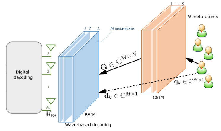
Figure 1: A BSIM and CSIM-assisted mMIMO system with multiple users.

II-A System Model

We consider the uplink of a multiuser MISO wireless system, where the BS is equipped with a large number of $M_{\mathrm{BS}}$ antennas that serve $K$ single-antennas users under the same time-frequency resources. In this context, we employ the BSIM, integrated into the BS to enable receive decoding in the EM wave domain, and the CSIM to enhance the communication between the users and the BS in the wave domain, as shown in Fig. 1. For the fabrication of BSIM, we utilize an array of $L$ metasurfaces, where each one of them consists of $M$ meta-atoms. The corresponding sets are $\mathcal{L}=\{1,\ldots,L\}$ and $\mathcal{M}=\{1,\ldots,M\}$. Similarly, the CSIM includes an array of $S$ metasurfaces, each including $N$ meta-atoms. The corresponding sets are $\mathcal{S}=\{1,\ldots,S\}$ and $\mathcal{N}=\{1,\ldots,N\}$. Both SIMs are connected to independent smart controllers, which can adjust the corresponding phase shifts of the EM waves that are transmitted through each of their meta-atoms. Note that the forward propagation process in each SIM resembles a fully connected ANN, where training the interconnection architecture of the BSIM enables uplink decoding, while the respective training of the CSIM enables shaping the propagation environment. We denote ${\bm{\Phi}}^{l}=\text{diag}\left(\right)({\bm{\phi}}^{l})\in\mathbb{C}^{M\times M}$, where ${\bm{\phi}}^{l}=[\phi^{l}_{1},\dots,\phi^{l}_{M}]^{{\scriptscriptstyle\mathsf{T}}}\in\mathbb{C}^{N\times 1}$ is the transmission coefficient matrix of the BSIM. Note that $\phi_{m}^{l}=e^{j\theta_{m}^{l}}$, where $\theta_{m}^{l}\in[0,2\pi),m\in\mathcal{M},l\in\mathcal{L}$ is the phase shift by the $m$-th meta-atom on the $k$-th transmit metasurface layer. Similarly, for the CSIM, we denote ${\bm{\Lambda}}^{s}=\text{diag}\left(\right)({\bm{\lambda}}^{s})\in\mathbb{C}^{M\times N}$, where ${\bm{\lambda}}^{s}=[\lambda^{s}_{1},\dots,\lambda^{s}_{M}]^{{\scriptscriptstyle\mathsf{T}}}\in\mathbb{C}^{N\times 1}$. Here, $\lambda_{n}^{s}=e^{j\xi_{n}^{s}}$ with $\xi_{n}^{s}\in[0,2\pi),n\in\mathcal{N},s\in\mathcal{S}$ being the phase shift by the $n$-th meta-atom on the $s$-th CSIM metasurface layer.

II-B Channel Model

The transmission coefficient from the $\tilde{m}$th meta-atom on the $(l-1)$st BSIM metasurface layer to the $m$th meta-atom on the $l$th BSIM metasurface layer, provided by the Rayleigh-Sommerfeld diffraction theory [19], is written as

$$w_{m,\tilde{m}}^{l}=\frac{A_{t}\cos x_{m,\tilde{m}}^{l}}{r_{m,\tilde{m}}^{l}}\left(\frac{1}{2\pi r^{l}_{m,\tilde{m}}}-j\frac{1}{\lambda}\right)e^{j2\pi r_{m,\tilde{m}}^{l}/\lambda},l\in\mathcal{L},$$ (1)

where $A_{t}$ expresses the area of each meta-atom, $x_{m,\tilde{m}}^{l}$ is the angle between the propagation direction and the normal direction of the $(l-1)$th BSIM metasurface layer, and $r_{m,\tilde{m}}^{l}$, is the corresponding transmission distance. As a result, the effect of the BSIM can be modeled as

$${\mathbf{P}}={\bm{\Phi}}^{L}{\mathbf{W}}^{L}\cdots{\bm{\Phi}}^{2}{\mathbf{W}}^{2}{\bm{\Phi}}^{1}\in\mathbb{C}^{M\times M},$$ (2)

where ${\mathbf{W}}^{l}\in\mathbb{C}^{M\times M},l\in\mathcal{L}/\{1\}$ is the transmission coefficient matrix between the $(l-1)st$ BSIM metasurface layer and the $l$th transmit metasurface layer. Regarding ${\mathbf{W}}^{1}\in\mathbb{C}^{M\times M_{\mathrm{BS}}}$, it is the transmission coefficient matrix between the $M_{\mathrm{BS}}$ transmit antennas and the first metasurface layer of the BSIM.

In the CSIM, the transmission coefficient from the $n$th meta-atom on the $s$th metasurface layer to the $\tilde{n}$th meta-atom on the $(s-1)$st metasurface layer can be written as

$$u_{\tilde{n},n}^{s}=\frac{A_{r}\cos\zeta_{\tilde{n},n}^{s}}{t_{\tilde{n},n}^{s}}\left(\frac{1}{2\pi t^{k}_{\tilde{n},n}}-j\frac{1}{\lambda}\right)e^{j2\pi t_{\tilde{n},n}^{s}/\lambda},s\in\mathcal{S},$$ (3)

where $A_{r}$ denotes the area of each meta-atom in the CSIM, $\zeta_{\tilde{n},n}^{s}$ expresses the angle between the propagation direction and the normal direction of the $(s-1)$th CSIM metasurface layer, and $t_{\tilde{n},n}^{s}$ is the corresponding transmission distance. In this case, the effect of the CSIM is described by

$${\mathbf{Z}}={\bm{\Lambda}}^{S}{\mathbf{U}}^{S}\cdots{\bm{\Lambda}}^{2}{\mathbf{U}}^{2}{\bm{\Lambda}}^{1}\in\mathbb{C}^{N\times N},$$ (4)

where ${\mathbf{U}}^{s}\in\mathbb{C}^{N\times N},s\in\mathcal{S}/\{1\}$ is the transmission coefficient matrix between the $s$th CSIM metasurface layer to the $(s-1)$st CSIM metasurface layer, and ${\mathbf{U}}^{1}\in\mathbb{C}^{N\times 1}$ is the transmission coefficient matrix from the output metasurface layer of the CSIM SIM to user $k$.

Based on narrowband quasi-static block fading channel modeling, we assume that the duration of each block is $\tau_{\mathrm{c}}$ channel uses. Also, by adopting the time-division-duplex (TDD) protocol as the recommended protocol for next-generation systems such as mMIMO systems, $\tau$ channel uses are allocated for the uplink training phase and $\tau_{\mathrm{c}}-\tau$ channel uses for the uplink data transmission phase.

Now, we denote ${\mathbf{G}}=[{\mathbf{g}}_{1}\ldots,{\mathbf{g}}_{N}]\in\mathbb{C}^{M\times N}$ the channel matrix between the BSIM and the CSIM, where ${\mathbf{g}}_{i}\in\mathbb{C}^{M\times 1}$ for $i\in\mathcal{N}$. Moreover, ${\mathbf{q}}_{k}\in\mathbb{C}^{N\times 1}$ expresses the channel between the CSIM and user $k$. Also, we assume the presence of a direct link between the BSIM and user $k$. We denote the corresponding link as ${\mathbf{d}}_{k}$. In this work, we assume the presence of realistic correlated Rayleigh fading, which occurs in practice [7]. The analysis with correlated Rician fading that includes a line-of-sight (LoS) component could be the topic of future work. Specifically, we have

$${\mathbf{G}} =\sqrt{\tilde{\beta}_{g}}{\mathbf{R}}_{\mathrm{BSIM}}^{1/2}{\mathbf{D}}{\mathbf{R}}_{\mathrm{CSIM}}^{1/2},$$ (5)

$${\mathbf{q}}_{k} =\sqrt{\tilde{\beta}_{k}}{\mathbf{R}}_{\mathrm{CSIM}}^{1/2}{\mathbf{c}}_{k},$$ (6)

$${\mathbf{d}}_{k} =\sqrt{\bar{\beta}_{k}}{\mathbf{R}}_{\mathrm{BSIM}}^{1/2}\bar{{\mathbf{c}}}_{k},$$ (7)

where ${\mathbf{R}}_{\mathrm{BSIM}}\in\mathbb{C}^{M\times M}$ and ${\mathbf{R}}_{\mathrm{CSIM}}\in\mathbb{C}^{N\times N}$ describe the correlation matrices at the BSIM and the CSIM respectively. Note that these matrices are deterministic Hermitian-symmetric positive semi-definite and are assumed to be known by the network. The spatial correlation matrices at the BSIM and CSIM are given by [7]

$$[{\mathbf{R}}_{\mathrm{BSIM}}]_{m,\tilde{m}} =\mathrm{sinc}(2r_{m,\tilde{m}}/\lambda),\tilde{m}\in\mathcal{M},m\in\mathcal{M},$$ (8)

$$[{\mathbf{R}}_{\mathrm{CSIM}}]_{\tilde{n},n} =\mathrm{sinc}(2t_{\tilde{n},n}/\lambda),n\in\mathcal{N},\tilde{n}\in\mathcal{N},$$ (9)

where $r_{m,\tilde{m}}$ and $t_{\tilde{n},n}$ are the corresponding meta-atom spacings. The path-losses $\tilde{\beta}_{g}$, $\bar{\beta}_{k}$, and $\tilde{\beta}_{k}$ correspond to BSIM-CSIM, CSIM-user $k$, and BSIM-user $k$ links, while ${\mathbf{c}}_{k}\sim\mathcal{CN}\left({\mathbf{0}},{\bm{\mathrm{I}}}_{N}\right)$, $\bar{{\mathbf{c}}}_{k}\sim\mathcal{CN}\left({\mathbf{0}},{\bm{\mathrm{I}}}_{M}\right)$, and $\mathrm{vec}({\mathbf{D}})\sim\mathcal{CN}\left({\mathbf{0}},{\bm{\mathrm{I}}}_{MN}\right)$ represent the small-scale fading parts. Contrary to most previous works, which assume that one of the links of the cascaded channels is deterministic, i.e., it represents a LoS component [24, 8], we consider a more general analysis, since we consider small-scale fading among all links.

By assuming that the phase shift matrices ${\bm{\Phi}}^{l},l\in\mathcal{L}$ and ${\bm{\Lambda}}^{s},s\in\mathcal{S}$ are given, the aggregated channel vector from the last BSIM layer to user $k$, includes the cascaded and direct channels, i.e., ${\mathbf{h}}_{k}={\mathbf{G}}{\mathbf{Z}}{\mathbf{U}}^{1}{\mathbf{q}}_{k}+{\mathbf{d}}_{k}\in\mathbb{C}^{M\times 1}$, which has a covariance matrix given by ${\mathbf{R}}_{k}=\mathbb{E}\{{\mathbf{h}}_{k}{\mathbf{h}}_{k}^{{\scriptscriptstyle\mathsf{H}}}\}$. Specifically, we have

$${\mathbf{R}}_{k} =\hat{\beta}_{k}\mathbb{E}\{{\mathbf{G}}{\mathbf{Z}}{\mathbf{U}}^{1}\mathbb{E}\{{\mathbf{q}}_{k}{\mathbf{q}}_{k}^{{\scriptscriptstyle\mathsf{H}}}\}{\mathbf{U}}^{1^{{\scriptscriptstyle\mathsf{H}}}}{\mathbf{Z}}^{{\scriptscriptstyle\mathsf{H}}}{\mathbf{G}}^{{\scriptscriptstyle\mathsf{H}}}\}+\bar{\beta}_{k}{\mathbf{R}}_{\mathrm{BSIM}}$$ (10)

$$=\hat{\beta}_{k}\mathbb{E}\{{\mathbf{G}}{\mathbf{Z}}{\mathbf{U}}^{1}{\mathbf{R}}_{\mathrm{CSIM}}{\mathbf{U}}^{1^{{\scriptscriptstyle\mathsf{H}}}}{\mathbf{Z}}^{{\scriptscriptstyle\mathsf{H}}}{\mathbf{G}}^{{\scriptscriptstyle\mathsf{H}}}\}+\bar{\beta}_{k}{\mathbf{R}}_{\mathrm{BSIM}}$$ (11)

$$=\hat{\beta}_{k}\tr({\mathbf{R}}_{\mathrm{CSIM}}{\mathbf{Z}}\bar{{\mathbf{R}}}_{\mathrm{CSIM}}{\mathbf{Z}}^{{\scriptscriptstyle\mathsf{H}}}){\mathbf{R}}_{\mathrm{BSIM}}+\bar{\beta}_{k}{\mathbf{R}}_{\mathrm{BSIM}},$$ (12)

where, in (10), we have applied the independence between ${\mathbf{G}}$ and ${\mathbf{q}}_{k}$, denoted $\hat{\beta}_{k}=\tilde{\beta}_{g}\tilde{\beta}_{k}$, and used $\mathbb{E}\{{\mathbf{d}}_{k}{\mathbf{d}}_{k}^{{\scriptscriptstyle\mathsf{H}}}\}=\bar{\beta}_{k}{\mathbf{R}}_{\mathrm{BSIM}}$. Next, we have used that $\mathbb{E}\{{\mathbf{q}}_{k}{\mathbf{q}}_{k}^{{\scriptscriptstyle\mathsf{H}}}\}=\tilde{\beta}_{k}{\mathbf{R}}_{\mathrm{CSIM}}$. In (12), we have denoted $\bar{{\mathbf{R}}}_{\mathrm{CSIM}}={\mathbf{U}}^{1}{\mathbf{R}}_{\mathrm{CSIM}}{\mathbf{U}}^{1^{{\scriptscriptstyle\mathsf{H}}}}$, and we have used the property $\mathbb{E}\{{\mathbf{V}}{\mathbf{U}}{\mathbf{V}}^{{\scriptscriptstyle\mathsf{H}}}\}=\tr({\mathbf{U}}){\bm{\mathrm{I}}}_{M}$, where ${\mathbf{U}}$ is a deterministic square matrix, and ${\mathbf{V}}$ is any matrix with independent and identically distributed (i.i.d.) entries of zero mean and unit variance.

III Channel Estimation and Uplink Data Transmission

III-A Channel Estimation

Given that perfect CSI is not attainable in practice, we employ the TDD protocol that considers an uplink training phase. In this phase, pilot symbols are transmitted to estimate the channel. However, a RIS has the peculiar characteristic that it cannot process any signals, i.e., it cannot obtain receive pilots and it cannot transmit them because it is implemented without any RF chains.

Herein, we propose a channel estimation method, where we estimate the aggregated channel as in [24, 8, 25] instead of the individual channels as in [13, 26, 27]. The latter approach comes with extra power and hardware cost. Moreover, the large dimension BSIM-CSIM channel would require a pilot overhead that would be prohibitively high if we estimated the individual channels. Also, we manage to express the estimated channel in closed form. Hence, the proposed method follows.

During the training phase, which lasts $\tau$ channel uses, it is assumed that all users send orthogonal pilot sequences. In particular, ${\mathbf{x}}_{k}=[x_{k,1},\ldots,x_{k,\tau}]^{{\scriptscriptstyle\mathsf{H}}}\in\mathbb{C}^{\tau\times 1}$ with ${\mathbf{x}}_{k}^{{\scriptscriptstyle\mathsf{H}}}{\mathbf{x}}_{l}=0~{}\forall k\neq l$ and ${\mathbf{x}}_{k}^{{\scriptscriptstyle\mathsf{H}}}{\mathbf{x}}_{k}=\tau\rho$ joules denotes the pilot sequence of user $k$, where all users use the same normalized signal-to-noise ratio (SNR) $\rho$ for transmitting each pilot symbol during the training phase.

Overall, the BS receives

$${\mathbf{Y}}^{\tr}=\sum_{i=1}^{K}{\mathbf{W}}^{1^{{\scriptscriptstyle\mathsf{H}}}}{\mathbf{P}}^{H}{\mathbf{h}}_{i}{\mathbf{x}}_{i}^{{\scriptscriptstyle\mathsf{H}}}+{\mathbf{Z}}^{\tr},$$ (13)

with ${\mathbf{Z}}^{\tr}\in\mathbb{C}^{M\times\tau}$ being the received AWGN matrix having independent columns with each one distributed as $\mathcal{CN}\left({\mathbf{0}},{\bm{\mathrm{I}}}_{M}\right)$.

By multiplying (13) with ${\mathbf{x}}_{k}$, we obtain

$${\mathbf{r}}_{k}={\mathbf{c}}_{k}+\frac{{\mathbf{z}}_{k}}{\tau\rho},$$ (14)

where ${\mathbf{c}}_{k}={\mathbf{W}}^{1^{{\scriptscriptstyle\mathsf{H}}}}{\mathbf{P}}^{H}{\mathbf{h}}_{k}$ and ${\mathbf{z}}_{k}={\mathbf{Z}}^{\tr}{\mathbf{x}}_{k}$.

Based on linear MMSE estimation, the overall perfect channel can be written as

$${\mathbf{c}}_{k}=\hat{{\mathbf{c}}}_{k}+\tilde{{\mathbf{c}}}_{k},$$ (15)

where $\hat{{\mathbf{c}}}_{k}$ and $\tilde{{\mathbf{c}}}_{k}$ are channel estimate and the estimation channel error vectors, respectively. The following lemma provides the linear MMSE estimated channel. Note that $\hat{{\mathbf{c}}}_{k}$ and $\tilde{{\mathbf{c}}}_{k}$ are uncorrelated and each of them has zero mean, but they are not independent [28].

Lemma 1

The linear MMSE estimated channel ${\mathbf{c}}_{k}$ of user $k$ at the BS is obtained as

$$\hat{{\mathbf{c}}}_{k}=\hat{{\mathbf{R}}}_{k}{\mathbf{Q}}_{k}{\mathbf{r}}_{k},$$ (16)

where $\hat{{\mathbf{R}}}_{k}={\mathbf{W}}^{1^{{\scriptscriptstyle\mathsf{H}}}}{\mathbf{P}}^{H}{\mathbf{R}}_{k}{\mathbf{W}}^{1}{\mathbf{P}}$, ${\mathbf{Q}}_{k}\!=\!\left(\!\hat{{\mathbf{R}}}_{k}\!+\!\frac{\sigma^{2}}{\tau\rho}{\bm{\mathrm{I}}}_{M}\!\right)^{\!-1}$, and ${\mathbf{r}}_{k}$ is the noisy channel given by (14).

Proof:

Please see Appendix A. ∎

The covariances of $\hat{{\mathbf{g}}}_{k}$ and $\tilde{{\mathbf{g}}}_{k}$ are easily obtained as

$${\bm{\Psi}}_{k}\! =\!\hat{{\mathbf{R}}}_{k}{\mathbf{Q}}_{k}\hat{{\mathbf{R}}}_{k},$$ (17)

$$\tilde{{\bm{\Psi}}}_{k} =\hat{{\mathbf{R}}}_{k}-{\bm{\Psi}}_{k}.$$ (18)

As can be seen, in this method, the length of the pilot sequence depends only on the number of users $K$, and is independent of the number of surfaces and elements at the BSIM and CSIM, which are generally large. Thus, we achieve substantial overhead reduction compared to estimating the individual channel, where the complexity would increase with increasing SIMs sizes. Also, we achieved to obtain the estimated overall channel in closed form instead of works such as [22] that cannot result in analytical expressions.

Another benefit of the proposed two-timescale method is that the channel is required to be estimated when the large-scale statistics (statistical CSI) varies, which is at every several coherence intervals. On the contrary, instantaneous CSI-based approaches would require channel estimation at every coherence interval that would result in high power consumption and computational complexity.

III-B Uplink Data Transmission

In this subsection, we provide the derivation of the uplink achievable sum SE of a SIM-assisted mMIMO system.

During the uplink data transmission phase, the BS receives

$${\mathbf{y}}=\sqrt{\rho}\sum_{i=1}^{K}{\mathbf{W}}^{1^{{\scriptscriptstyle\mathsf{H}}}}{\mathbf{P}}^{H}{\mathbf{h}}_{i}s_{i}+{\mathbf{n}},$$ (19)

where ${\mathbf{n}}\sim\mathcal{CN}\left({\mathbf{0}},{\bm{\mathrm{I}}}_{M}\right)$ is the AWGN at the BS, $s_{i}\sim\mathcal{CN}(0,1)$ is the transmit signal vector, $\rho$ is the uplink SNR, and ${\mathbf{h}}_{i}$ is the aggregated channel from the last BSIM layer to user $i$.

After application of a receive combining vector ${\mathbf{v}}_{k}$ as $\hat{s}_{k}={\mathbf{v}}_{k}^{{\scriptscriptstyle\mathsf{H}}}{\mathbf{y}}$, the BS obtains $s_{k}$ from user $k$ as

$$\hat{s}_{k} =\sqrt{\rho}\mathbb{E}\left\{{\mathbf{v}}_{k}^{{\scriptscriptstyle\mathsf{H}}}{\mathbf{W}}^{1^{{\scriptscriptstyle\mathsf{H}}}}{\mathbf{P}}^{H}{{\mathbf{h}}}_{k}\right\}s_{k}$$

$$+\sqrt{\rho}\left({\mathbf{v}}_{k}^{{\scriptscriptstyle\mathsf{H}}}{\mathbf{W}}^{1^{{\scriptscriptstyle\mathsf{H}}}}{\mathbf{P}}^{H}{{\mathbf{h}}}_{k}-\mathbb{E}\left\{{\mathbf{v}}_{k}^{{\scriptscriptstyle\mathsf{H}}}{\mathbf{W}}^{1^{{\scriptscriptstyle\mathsf{H}}}}{\mathbf{P}}^{H}{{\mathbf{h}}}_{k}\right\}\right)s_{k}$$

$$+\sum_{i\neq k}^{K}\sqrt{\rho}{\mathbf{v}}_{k}^{{\scriptscriptstyle\mathsf{H}}}{\mathbf{W}}^{1^{{\scriptscriptstyle\mathsf{H}}}}{\mathbf{P}}^{H}{{\mathbf{h}}}_{i}s_{i}+{\mathbf{v}}_{k}^{{\scriptscriptstyle\mathsf{H}}}{\mathbf{n}},$$ (20)

where we have also accounted for channel hardening, which is applicable in mMIMO systems with $M>8$ [28]. In (20), the first term is the desired signal, the second term is the beamforming gain uncertainty, the third term is multiuser interference, and the last term is the post-processed AWGN noise.

Next, we derive the use-and-then-forget bound on the uplink average SE, which is a lower bound [28]. For this reason, we assume the worst-case uncorrelated additive noise scenario for the inter-user interference and the AWGN noise. In this case, the achievable SE can be written as

$$\mathrm{SE}_{k}=\frac{\tau_{\mathrm{c}}-\tau}{\tau_{\mathrm{c}}}\log_{2}\left(1+\gamma_{k}\right)\!,$$ (21)

where the fraction represents the percentage of samples transmitted during the uplink data transmission, and $\gamma_{k}=\frac{S_{k}}{I_{k}}$ denotes the uplink signal-to-interference-plus-noise ratio (SINR). Here, $S_{k}$ and $I_{k}$ describe the desired signal power and the interference plus noise power. In terms of ${\mathbf{g}}_{k}$, we have

$$S_{k} =\rho|\mathbb{E}\left\{{\mathbf{v}}_{k}^{{\scriptscriptstyle\mathsf{H}}}{\mathbf{c}}_{k}\right\}|^{2},$$ (22)

$$I_{k} =\mathbb{E}\left\{|{\mathbf{v}}_{k}^{{\scriptscriptstyle\mathsf{H}}}{\mathbf{c}}_{k}-\mathbb{E}\left\{{\mathbf{v}}_{k}^{{\scriptscriptstyle\mathsf{H}}}{\mathbf{c}}_{k}\right\}|^{2}\right\}+\sum_{i\neq k}^{K}\mathbb{E}\left\{|{\mathbf{v}}_{k}^{{\scriptscriptstyle\mathsf{H}}}{\mathbf{c}}_{i}|^{2}\right\}$$

$$+\!\mathbb{E}\left\{|{\mathbf{v}}_{k}^{{\scriptscriptstyle\mathsf{H}}}{\mathbf{n}}|^{2}\right\}\!.$$ (23)

In this work, we assume MRC decoding to provide a closed-form SE, i.e., ${\mathbf{v}}_{k}=\hat{{\mathbf{c}}}_{k}$.

Theorem 1

The uplink SINR of user $k$ for given SIMs in a BSIM and CSIM assisted mMIMO system is tightly approximated as

$$\gamma_{k}\ {\color[rgb]{0,0,0}\approx}\ \frac{S_{k}}{\color[rgb]{0,0,0}\tilde{I}_{k}},$$ (24)

where

$${S}_{k} =\tr^{2}\left({\bm{\Psi}}_{k}\right)\!,$$ (25)

$$\tilde{I}_{k} =\sum_{i=1}^{K}\tr\!\left(\hat{{\mathbf{R}}}_{i}{\bm{\Psi}}_{k}\right)-\tr\left({\bm{\Psi}}_{k}^{2}\right)+\frac{1}{\rho}\tr({\bm{\Psi}}_{k}).$$ (26)

Proof:

Please see Appendix B. ∎

Theorem 1 provides a tight approximation as the numerical results in Section LABEL:Numerical reveal. The tightness is also expected because it comes as a result of the exploitation of channel hardening appearing in mMIMO systems [28].

IV Problem Formulation and Optimization

It is crucial to optimize the sum SE in terms of the phase shift matrices of the SIMs included in the proposed architecture.

IV-A Problem Formulation

By assuming infinite-resolution phase shifters, the formulation of the optimization problem follows as

(27a)

(27b)

(27c)

(27d)

(27e)

In problem $(\mathcal{P})$, we have denote $f({\bm{\phi}}_{l},{\bm{\lambda}}_{s})$ the objective function that includes the approximate of the SINR provided by Theorem (1).

IV-B Simultaneous Optimization of Both SIMs

The non-convexity of problem $(\mathcal{P})$ and the coupling between the optimization variables of the two SIMs, which also have constant modulus constraints lead us to seek a locally optimal solution. Note that many previous optimization methods on RIS-aided systems have applied alternating optimization (AO) to optimize the relevant variables in each case [5, 32]. Although AO-based methods can be implemented easily, their convergence may require many iterations, which increase with increasing the size of RIS [33]. Since SIM-assisted systems are expected to include a large number of elements, the AO methods is not suggested.

Given that the projection operators can be obtained in closed form, we can apply the projected gradient ascent method (PGAM) [34, Ch. 2] for the simultaneous optimization of ${\bm{\phi}}_{l}$ and ${\bm{\lambda}}_{s}$ instead of the AO method. Numerical results in Section 27bk will demonstrate the superiority of the proposed approach.

IV-C Proposed Algorithm-PGAM

According to the proposed PGAM, starting from $({\bm{\phi}}_{l}^{0},{\bm{\lambda}}_{l}^{0})$, we shift towards the gradient of the objective function, i.e., $\nabla f({\bm{\phi}}_{l},{\bm{\lambda}}_{s})$, where the rate of change of $f({\bm{\phi}}_{l},{\bm{\lambda}}_{s})$ becomes maximum. The newly computed points ${\bm{\phi}}_{l}$ and ${\bm{\lambda}}_{s}$ are projected onto $\Phi_{l}$ and $\Lambda_{s}$, respectively to keep the updated points inside the feasible set.

The step size of this shift is determined by a parameter $\mu>0$. For the sake of description, we define the following sets.

$$\Phi_{l} =\{{\bm{\phi}}_{l}\in\mathbb{C}^{M\times 1}:|\phi^{l}_{i}|=1,i=1,\ldots,M\},$$ (27ab)

$$\Lambda_{s} =\{{\bm{\lambda}}_{s}\in\mathbb{C}^{N\times 1}:|\lambda^{s}_{i}|=1,i=1,\ldots,N\}.$$ (27ac)

The proposed PGAM solving (27) is outlined in Algorithm 1. As can be seen, the algorithm includes the following two iterations.

$${\bm{\phi}}_{l}^{i+1} =P_{\Phi_{l}}({\bm{\phi}}_{l}^{i}+\mu_{i}\nabla_{{\bm{\phi}}_{l}}f({\bm{\phi}}_{l}^{i},{\bm{\lambda}}_{s}^{i}))$$ (27ad)

$${\bm{\lambda}}_{s}^{i+1} =P_{\Lambda_{s}}({\bm{\lambda}}_{s}^{i}+\mu_{i}\nabla_{{\bm{\lambda}}_{s}}f({\bm{\phi}}_{l}^{i},{\bm{\lambda}}_{s}^{i})),$$ (27ae)

where $P_{\Phi_{l}}(\cdot)$ and $P_{\Lambda_{s}}(\cdot)$ are the projections onto $\Phi_{l}$ and $\Lambda_{s}$, respectively. Also, to find the step size, we apply the Armijo-Goldstein backtracking line search. For this reason, we define the quadratic approximation of $f({\bm{\phi}}_{l},{\bm{\lambda}}_{s})$ as

$$Q_{\mu}({\bm{\phi}}_{l},{\bm{\lambda}}_{s};{\mathbf{x}},{\mathbf{y}})=f({\bm{\phi}}_{l},{\bm{\lambda}}_{s})+\langle\nabla_{{\bm{\phi}}_{l}}f({\bm{\phi}}_{l},{\bm{\lambda}}_{s}),{\mathbf{x}}-{\bm{\phi}}_{l}\rangle$$

$$-\frac{1}{\mu}\|{\mathbf{x}}-{\bm{\phi}}_{l}\|^{2}_{2}+\langle\nabla_{{\bm{\lambda}}_{s}}f({\bm{\phi}}_{l},{\bm{\lambda}}_{s}),{\mathbf{y}}-{\bm{\lambda}}_{s}\rangle$$

$$-\frac{1}{\mu}\|{\mathbf{y}}-{\bm{\lambda}}_{s}\|^{2}_{2}.$$ (27af)

The step size in (27ad) and (27ae) can be found as $\mu_{i}=L_{i}\kappa^{m_{i}}$ with $L_{i}>0$, and $\kappa\in(0,1)$, where the parameter $m_{n}$ is the smallest nonnegative integer satisfying

$$f({\bm{\phi}}_{l}^{i+1},{\bm{\lambda}}_{s}^{i+1})\geq Q_{L_{i}\kappa^{m_{i}}}({\bm{\phi}}_{l}^{i},{\bm{\lambda}}_{s}^{i};{\bm{\phi}}_{l}^{i+1},{\color[rgb]{0,0,0}{\bm{\lambda}}_{s}^{i+1}}),$$ (27ag)

which can be performed by an iterative procedure.

Algorithm 1 Simultaneous PGAM for both SIMS

1:  Input: ${\bm{\phi}}_{l}^{0},{\bm{\lambda}}_{s}^{0},\mu_{1}>0$, $\kappa\in(0,1)$

2:  $i\leftarrow 1$

3:  repeat

4:     repeat

5:        ${\bm{\phi}}_{l}^{i+1}=P_{\Phi_{l}}({\bm{\phi}}_{l}^{i}+\mu_{ni}\nabla_{{\bm{\phi}}_{l}}f({\bm{\phi}}_{l}^{i},{\bm{\lambda}}_{s}^{i}))$

6:        ${\bm{\lambda}}_{s}^{i+1}=P_{\Lambda_{s}}({\bm{\lambda}}_{s}^{i}+\mu_{i}\nabla_{{\bm{\lambda}}_{s}}f({\bm{\phi}}_{l}^{i},{\bm{\lambda}}_{s}^{i}))$

7:        if  $f({\bm{\phi}}_{l}^{i+1},{\bm{\lambda}}_{s}^{i+1})\leq Q_{\mu_{i}}({\bm{\phi}}_{l}^{i},{\bm{\lambda}}_{s}^{i};{\bm{\phi}}_{l}^{i+1},{\color[rgb]{0,0,0}{\bm{\lambda}}_{s}^{i+1}})$ then

8:           $\mu_{i}=\mu_{i}\kappa$

9:        end if

10:     until  $f({\bm{\phi}}_{l}^{i+1},{\bm{\lambda}}_{s}^{i+1})>Q_{\mu_{i}}({\bm{\phi}}_{l}^{i},{\bm{\lambda}}_{s}^{i};{\bm{\phi}}_{l}^{i+1},{\bm{\lambda}}_{s}^{i+1})$

11:     $\mu_{i+1}\leftarrow\mu_{i}$

12:     $i\leftarrow i+1$

13:  until  convergence

14:  Output: ${\bm{\phi}}_{l}^{i+1},{\bm{\lambda}}_{s}^{i+1}$

IV-D Complex-valued Gradients

Below, we present the gradients $\nabla_{{\bm{\phi}}_{l}}f({\bm{\phi}}_{l},{\bm{\lambda}}_{s})$ and $\nabla_{{\bm{\lambda}}_{s}}f({\bm{\phi}}_{l},{\bm{\lambda}}_{s})$.

Proposition 1

The gradients of $f({\bm{\phi}}_{l},{\bm{\lambda}}_{s})$ regarding ${\bm{\phi}}_{l}^{*}$ and ${\bm{\lambda}}_{s}^{*}$ are provided closed-forms by

$$\nabla_{{\bm{\phi}}_{l}}f({\bm{\phi}}_{l},{\bm{\lambda}}_{s}) =\frac{\tau_{c}-\tau}{\tau_{c}\log_{2}(e)}\sum_{k=1}^{K}\frac{\tilde{I}_{k}\nabla_{{\bm{\phi}}_{l}}S_{k}-S_{k}\nabla_{{\bm{\phi}}_{l}}\tilde{I}_{k}}{(1+\gamma_{k})\tilde{I}_{k}},$$ (27ah)

$$\nabla_{{\bm{\lambda}}_{s}}f({\bm{\phi}}_{l},{\bm{\lambda}}_{s}) =\frac{\tau_{c}-\tau}{\tau_{c}\log_{2}(e)}\sum_{k=1}^{K}\frac{\tilde{I}_{k}\nabla_{{\bm{\lambda}}_{s}}S_{k}-S_{k}\nabla_{{\bm{\lambda}}_{s}}\tilde{I}_{k}}{(1+\gamma_{k})\tilde{I}_{k}},$$ (27ai)

where

Figure 2:

V-C Sum SE Performance Evaluation

First, Figs. V-C.(a) and V-C.(b) illustrate the sum SE versus the numbers of meta-atoms $M$ and $N$ on each metasurface layer of the BSIM and CSIM, respectively. In both figures, we observe an increase in the sum SE with the sizes of the corresponding surfaces. However, the impact of the CSIM is greater since a double increase in $N$ results in $170\%$ improvement compared to $200\%$ improvement when $M$ becomes almost double (from $40$ to $100$). Also, in Fig.V-C.(b), we observe the impact of the CSIM. In particular, we have shown the SE when the CSIM is absent, and only the direct signal exists, the performance is quite low.

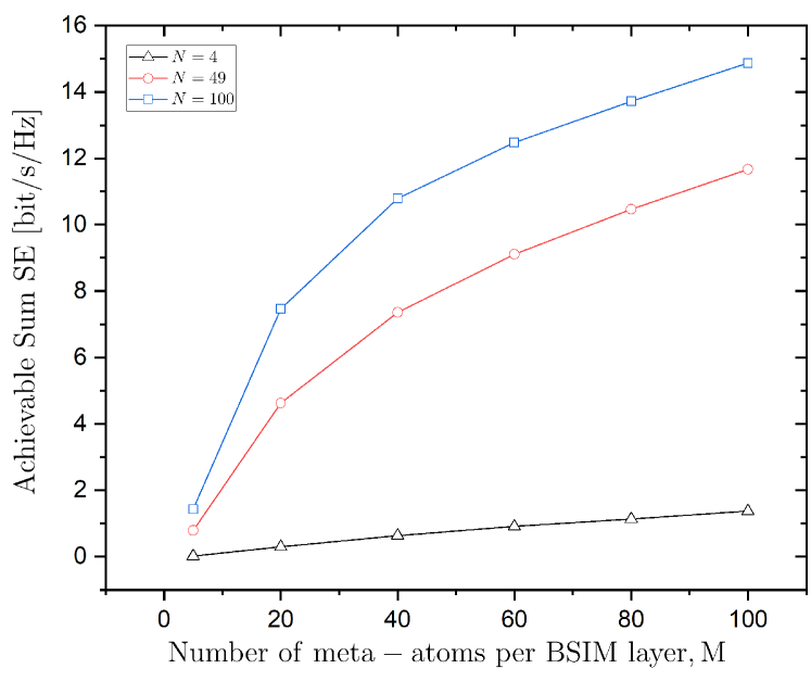
(a) Achievable sum SE of the proposed double-SIM mMIMO architecture versus the number of meta-atoms of the BSIM $M$ while varying the number of meta-atoms of the CSIM $N$.

Figure 3:

Figs. V-C.(a) and V-C.(b) depict the sum SE versus the numbers of layers $L$ and $S$ of the BSIM and CSIM, respectively. In Fig. V-C.(a), we observe that the sum SE improves until $L=4$ because of the ability of the BSIM to mitigate the inter-user interference in the EM wave domain. In Fig. V-C.(b), it is shown that the sum SE increases with the number of metasurfaces $S$ due to increasing array and multiplexing gains. In both figures, a significant improvement is observed compared to the single-layer BSIM and CSIM, respectively. However, this improvement in the BSIM is greater.

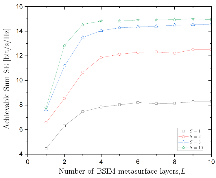
(a) Achievable sum SE of the proposed double-SIM mMIMO architecture versus the number of metasurfaces of the BSIM $L$ while varying the number of metasurfaces of the CSIM $S$.

Figure 4:

In Fig. 7, we show the sum SE versus the number of users $K$. We observe that the sum SE grows with $K$ at the beginning but decreases after a certain value of $K$. The reason behind this observation is that the increase in the beginning comes from the increase of the spatial multiplexing gain with $K$. Later, the increase of inter-user interference due to increasing $K$ cannot be mitigated by the BSIM and its wave-based decoding. Based on our setup, the BSIM can mitigate the multiuser interference of maximum $K=5$ users. Moreover, we observe that an increase in the number of meta-atoms $M$ of the BSIM can serve a larger number of users.

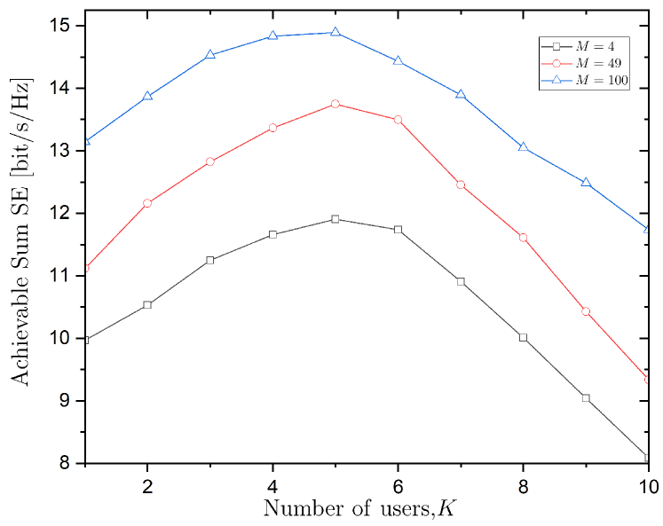
Figure 5: Achievable sum SE of the proposed double-SIM mMIMO architecture versus the number of users $K$ while varying the number of BCSIM meta-atoms $M$.

Fig. 6 depicts the sum SE versus the transmit SNR for various cases regarding the values of the phase shifts of the BSIM. The optimal phase shifts design achieves the best performance as expected. The designs with random phase shifts and equal phase shifts follow with lower performance. In parallel, Monte Carlo simulations verify the analytical results.

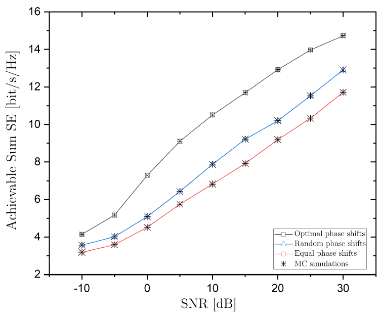
Figure 6: Achievable sum SE of the proposed double-SIM mMIMO architecture versus the SNR for different cases regarding the phase shifts.

In Fig. 7, we present a comparison between the BCIM and CSIM-assisted mMIMO system with the case where the BSIM is replaced by a conventional BS that employs a conventional zero-forcing (ZF) decoder for mitigating the multiuser interference. For the sake of a fair comparison, we assume that the path loss corresponding to user $k$ is $d_{k}=\sqrt{H_{\mathrm{BS}^{2}}+(d_{0}(k-1))^{2}}$. The conventional BS requires $M_{\mathrm{BS}}=16$ antennas to exhibit better performance than the BSIM with $M_{\mathrm{BS}}=64$ and $M=49$ elements. In other words, we can remove completely the digital decoding at the BS while equipping each antenna with low-resolution ADCs/DACs that can reduce overall the energy consumption and hardware cost.

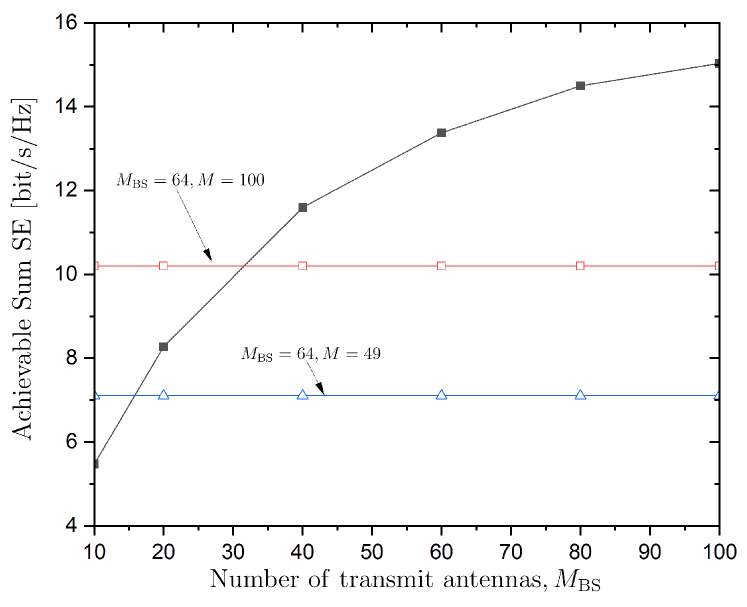
Figure 7: Achievable sum SE of the proposed double-SIM mMIMO architecture versus the number of BS antennas $M_{\mathrm{BS}}$ while varying the number of receiver metasurface layers $K$.

VI Conclusion

In this paper, a novel SIM-assisted mMIMO architecture was proposed. In particular, a SIM enables wave-based decoding in the uplink, and another SIM is used at the intermediate space between the users and the BS to increase further the ability of the proposed configuration to reshape the surrounding EM environment. We first suggested a channel estimation scheme, which obtains the estimated channel in closed form in a single phase. Then, we derived the uplink sum SE, and optimized both SIMs simultaneously. Simulations showed the superiority of the proposed architecture compared to counterparts, demonstrated the impact of various parameters on the sum SE, and exhibited outperformance against the AO method, where the SIMs are optimized separately. For example, an increase in the numbers of layers and meta-atoms increases the performance. Especially, the BSIM exhibits interference cancellation. Also, the proposed architecture is superior to the conventional digital MISO counterpart, which means that SIM-based designs could lead to next-generation energy-efficient networks.

Appendix A Proof of Lemma 1

The LMMSE estimator of ${\mathbf{c}}_{k}={\mathbf{W}}^{1^{{\scriptscriptstyle\mathsf{H}}}}{\mathbf{P}}^{H}{\mathbf{h}}_{k}$ is derived according to according to [35, Ch. 12] as

$$\hat{{\mathbf{c}}}_{k}=\mathbb{E}\{{\mathbf{r}}_{k}{\mathbf{g}}_{k}^{{\scriptscriptstyle\mathsf{H}}}\}\left(\mathbb{E}\{{\mathbf{r}}_{k}{\mathbf{r}}_{k}^{{\scriptscriptstyle\mathsf{H}}}\}\right)^{-1}.$$ (27at)

The first term of (27at) is written as

$$\mathbb{E}\{{\mathbf{r}}_{k}{\mathbf{c}}_{k}^{{\scriptscriptstyle\mathsf{H}}}\} =\mathbb{E}\big{[}\big{(}{\mathbf{W}}^{1^{{\scriptscriptstyle\mathsf{H}}}}{\mathbf{P}}^{H}{\mathbf{c}}_{k}+\frac{{\mathbf{z}}_{k}}{\tau\rho}\big{)}{\mathbf{c}}_{k}^{{\scriptscriptstyle\mathsf{H}}}{\mathbf{W}}^{1}{\mathbf{P}}\big{]}$$ (27au)

$$={\mathbf{W}}^{1^{{\scriptscriptstyle\mathsf{H}}}}{\mathbf{P}}^{H}\mathbb{E}\{{\mathbf{c}}_{k}{\mathbf{c}}_{k}^{{\scriptscriptstyle\mathsf{H}}}\}{\mathbf{W}}^{1}{\mathbf{P}}={\mathbf{W}}^{1^{{\scriptscriptstyle\mathsf{H}}}}{\mathbf{P}}^{H}{\mathbf{R}}_{k}{\mathbf{W}}^{1}{\mathbf{P}}.$$ (27av)

The second term is obtained as

$$\mathbb{E}\{{\mathbf{r}}_{k}{\mathbf{r}}_{k}^{{\scriptscriptstyle\mathsf{H}}}\} ={\mathbf{W}}^{1^{{\scriptscriptstyle\mathsf{H}}}}{\mathbf{P}}^{H}{\mathbf{R}}_{k}{\mathbf{W}}^{1}{\mathbf{P}}+\frac{\sigma^{2}}{\tau\rho}{\bm{\mathrm{I}}}_{M}.$$ (27aw)

By inserting (27av) and (27aw) into (27at), we obtain

$$\hat{{\mathbf{c}}}_{k}=\hat{{\mathbf{R}}}_{k}{\mathbf{Q}}_{k}{\mathbf{r}}_{k},$$ (27ax)

where $\hat{{\mathbf{R}}}_{k}={\mathbf{W}}^{1^{{\scriptscriptstyle\mathsf{H}}}}{\mathbf{P}}^{H}{\mathbf{R}}_{k}{\mathbf{W}}^{1}{\mathbf{P}}$ and ${\mathbf{Q}}_{k}\!=\!\left(\!\hat{{\mathbf{R}}}_{k}\!+\!\frac{\sigma^{2}}{\tau\rho}{\bm{\mathrm{I}}}_{M}\!\right)^{\!-1}$.

Appendix B Proof of Theorem 1

Regarding the desired signal power part, we have

$$\mathbb{E}\left\{{\mathbf{v}}_{k}^{{\scriptscriptstyle\mathsf{H}}}{\mathbf{c}}_{k}\right\} =\tr(\mathbb{E}\{{\mathbf{c}}_{k}\hat{{\mathbf{c}}}_{k}\})$$

$$=\tr(\mathbb{E}\{{\mathbf{c}}_{k}\hat{{\mathbf{R}}}_{k}{\mathbf{Q}}_{k}{\mathbf{r}}_{k}\})$$ (27ay)

$$=\tr({\bm{\Psi}}_{k}),$$ (27az)

where, in (27ay), we have inserted (20), while in the last equation, we have computed the expectation between ${\mathbf{c}}_{k}$ and ${\mathbf{r}}_{k}$, and we have used (17).

In the case of $I_{k}$, the first term can be written as

$$\!\!\mathbb{E}\left\{|\hat{{\mathbf{c}}}_{k}^{{\scriptscriptstyle\mathsf{H}}}{\mathbf{c}}_{k}-\mathbb{E}\left\{\hat{{\mathbf{c}}}_{k}^{{\scriptscriptstyle\mathsf{H}}}{\mathbf{c}}_{k}\right\}|^{2}\right\}\!=\!\mathbb{E}\big{\{}\big{|}\hat{{\mathbf{c}}}_{k}^{{\scriptscriptstyle\mathsf{H}}}{\mathbf{c}}_{k}\big{|}^{2}\big{\}}\!-\!\big{|}\mathbb{E}\left\{\hat{{\mathbf{c}}}_{k}^{{\scriptscriptstyle\mathsf{H}}}{\mathbf{c}}_{k}\right\}\big{|}^{2}$$ (27ba)

$$=\mathbb{E}\big{\{}\big{|}\hat{{\mathbf{c}}}_{k}^{{\scriptscriptstyle\mathsf{H}}}\hat{{\mathbf{c}}}_{k}+\hat{{\mathbf{c}}}_{k}^{{\scriptscriptstyle\mathsf{H}}}\tilde{{\mathbf{c}}}_{k}\big{|}^{2}\big{\}}-\big{|}\mathbb{E}\big{\{}\hat{{\mathbf{c}}}_{k}^{{\scriptscriptstyle\mathsf{H}}}\hat{{\mathbf{c}}}_{k}\big{\}}\big{|}^{2}$$ (27bb)

$$=\mathbb{E}\big{\{}\big{|}\hat{{\mathbf{c}}}_{k}^{{\scriptscriptstyle\mathsf{H}}}\tilde{{\mathbf{c}}}_{k}\big{|}^{2}\big{\}}+2\real\{\mathbb{E}\{\hat{{\mathbf{c}}}_{k}^{{\scriptscriptstyle\mathsf{H}}}\hat{{\mathbf{c}}}_{k}\hat{{\mathbf{c}}}_{k}^{{\scriptscriptstyle\mathsf{H}}}\tilde{{\mathbf{c}}}_{k}\}\}$$ (27bc)

where in (27bb), we have substituted (15). The second term in (27bc) goes to zero according to the channel hardening property in mMIMO, which gives with high accuracy $\hat{{\mathbf{c}}}_{k}^{{\scriptscriptstyle\mathsf{H}}}\hat{{\mathbf{c}}}_{k}\approx\mathbb{E}\{\hat{{\mathbf{c}}}_{k}^{{\scriptscriptstyle\mathsf{H}}}\hat{{\mathbf{c}}}_{k}\}$ [28]. Specifically, the second term becomes

$$\mathbb{E}\{\hat{{\mathbf{c}}}_{k}^{{\scriptscriptstyle\mathsf{H}}}\hat{{\mathbf{c}}}_{k}\hat{{\mathbf{c}}}_{k}^{{\scriptscriptstyle\mathsf{H}}}\tilde{{\mathbf{c}}}_{k}\}\approx\mathbb{E}\{\hat{{\mathbf{c}}}_{k}^{{\scriptscriptstyle\mathsf{H}}}\hat{{\mathbf{c}}}_{k}\}\mathbb{E}\{\hat{{\mathbf{c}}}_{k}^{{\scriptscriptstyle\mathsf{H}}}\tilde{{\mathbf{c}}}_{k}\}=0.$$ (27bd)

Hence, (27bc) becomes

$$\!\!\mathbb{E}\big{\{}\big{|}\hat{{\mathbf{c}}}_{k}^{{\scriptscriptstyle\mathsf{H}}}{\mathbf{c}}_{k}-\mathbb{E}\big{\{}\hat{{\mathbf{c}}}_{k}^{{\scriptscriptstyle\mathsf{H}}}{\mathbf{c}}_{k}\big{\}}\big{|}^{2}\big{\}}\!\approx\!\mathbb{E}\big{\{}|\hat{{\mathbf{c}}}_{k}^{{\scriptscriptstyle\mathsf{H}}}\tilde{{\mathbf{c}}}_{k}|^{2}\big{\}}$$ (27be)

$$=\tr\!\left(\hat{{\mathbf{R}}}_{k}{\bm{\Psi}}_{k}\right)-\tr\left({\bm{\Psi}}_{k}^{2}\right).$$ (27bf)

For the derivation of (27bf), we apply the approximations $\hat{{\mathbf{c}}}_{k}^{{\scriptscriptstyle\mathsf{H}}}\hat{{\mathbf{c}}}_{k}\approx\mathbb{E}\{\hat{{\mathbf{c}}}_{k}^{{\scriptscriptstyle\mathsf{H}}}\hat{{\mathbf{c}}}_{k}\}$ and $\tilde{{\mathbf{c}}}_{k}^{{\scriptscriptstyle\mathsf{H}}}\tilde{{\mathbf{c}}}_{k}\approx\mathbb{E}\{\tilde{{\mathbf{c}}}_{k}^{{\scriptscriptstyle\mathsf{H}}}\tilde{{\mathbf{c}}}_{k}\}$ due to channel hardening. Thus, we result in

$$\mathbb{E}\{|\hat{{\mathbf{c}}}_{k}^{{\scriptscriptstyle\mathsf{H}}}\tilde{{\mathbf{c}}}_{k}|^{2}\} =\tr(\mathbb{E}\{\hat{{\mathbf{c}}}_{k}\hat{{\mathbf{c}}}_{k}^{{\scriptscriptstyle\mathsf{H}}}\tilde{{\mathbf{c}}}_{k}\tilde{{\mathbf{c}}}_{k}^{{\scriptscriptstyle\mathsf{H}}}\})$$ (27bg)

$$\approx\tr(\mathbb{E}\{\hat{{\mathbf{c}}}_{k}\hat{{\mathbf{c}}}_{k}^{{\scriptscriptstyle\mathsf{H}}}\}\mathbb{E}\{\tilde{{\mathbf{c}}}_{k}\tilde{{\mathbf{c}}}_{k}^{{\scriptscriptstyle\mathsf{H}}}\})$$ (27bh)

$$=\tr((\hat{{\mathbf{R}}}_{k}-{\bm{\Psi}}_{k}){\bm{\Psi}}_{k}).$$ (27bi)

The multiuser interference term in (23) becomes

$$\mathbb{E}\left\{|\hat{{\mathbf{c}}}_{k}^{{\scriptscriptstyle\mathsf{H}}}{\mathbf{c}}_{i}|^{2}\right\}=\mathbb{E}\big{\{}\big{|}\hat{{\mathbf{c}}}_{k}^{{\scriptscriptstyle\mathsf{H}}}(\hat{{\mathbf{c}}}_{i}+\tilde{{\mathbf{c}}}_{i})\big{|}^{2}\big{\}}$$ (27bj)

$$=\mathbb{E}\big{\{}\big{|}\hat{{\mathbf{c}}}_{k}^{{\scriptscriptstyle\mathsf{H}}}\hat{{\mathbf{c}}}_{i}\big{|}^{2}\big{\}}+\mathbb{E}\big{\{}\big{|}\hat{{\mathbf{c}}}_{k}^{{\scriptscriptstyle\mathsf{H}}}\tilde{{\mathbf{c}}}_{i}\big{|}^{2}\big{\}}+2\real\{\mathbb{E}\{\hat{{\mathbf{c}}}_{k}^{{\scriptscriptstyle\mathsf{H}}}\hat{{\mathbf{c}}}_{i}\tilde{{\mathbf{c}}}_{i}^{{\scriptscriptstyle\mathsf{H}}}\hat{{\mathbf{c}}}_{k}\}\}$$ (27bk)

$$=\tr\!\left({\bm{\Psi}}_{k}\hat{{\mathbf{R}}}_{i}\right),$$ (27bl)

where the third term in (27bl) is zero because it holds that

$$2\real\{\mathbb{E}\{\hat{{\mathbf{c}}}_{k}^{{\scriptscriptstyle\mathsf{H}}}\hat{{\mathbf{c}}}_{i}\tilde{{\mathbf{c}}}_{i}^{{\scriptscriptstyle\mathsf{H}}}\hat{{\mathbf{c}}}_{k}\}\} \!=\!2\real\left\{\mathbb{E}\{\tr\!\left(\!\left(\hat{{\mathbf{c}}}_{k}\hat{{\mathbf{c}}}_{k}^{{\scriptscriptstyle\mathsf{H}}}\right)\!\!\left(\tilde{{\mathbf{c}}}_{i}\hat{{\mathbf{c}}}_{i}^{{\scriptscriptstyle\mathsf{H}}}\right)\!\right)\!\right\}$$ (27bm)

$$\!=\!2\real\left\{\tr\!\left(\mathbb{E}\{\hat{{\mathbf{c}}}_{k}\hat{{\mathbf{c}}}_{k}^{{\scriptscriptstyle\mathsf{H}}}\}\mathbb{E}\{\tilde{{\mathbf{c}}}_{i}\hat{{\mathbf{c}}}_{i}^{{\scriptscriptstyle\mathsf{H}}}\}\right)\!\right\}$$ (27bn)

$$=0,$$ (27bo)

where, first, we used that $\hat{{\mathbf{c}}}_{k}$ and $\hat{{\mathbf{c}}}_{i}$ are independent, and next that $\tilde{{\mathbf{c}}}_{i}$ and $\hat{{\mathbf{c}}}_{i}$ are uncorrelated.

The last term in (23) is written as

$$\mathbb{E}\left\{|\hat{{\mathbf{c}}}_{k}^{{\scriptscriptstyle\mathsf{H}}}{\mathbf{n}}|^{2}\right\} =\tr(\mathbb{E}\{\hat{{\mathbf{c}}}_{k}\hat{{\mathbf{c}}}_{k}^{{\scriptscriptstyle\mathsf{H}}}\})$$ (27bp)

$$=\tr({\bm{\Psi}}_{k}),$$ (27bq)

where, in (27bp), we have used that $\hat{{\mathbf{c}}}_{k}$ and ${\mathbf{n}}$ are uncorrelated.

The combination of (27bf), (27bl), and (27bp) provides the approximate of ${I}_{k}$, which is $\tilde{I}_{k}$, and concludes the proof.

Appendix C Proof of Proposition 1

First, we focus on the derivation of $\nabla_{{\bm{\phi}}_{l}}f({\bm{\phi}}_{l},{\bm{\lambda}}_{s})$. From (27a), we can easily obtain

$$\nabla_{{\bm{\phi}}_{l}}f({\bm{\phi}}_{l},{\bm{\lambda}}_{s})=\frac{\tau_{c}-\tau}{\tau_{c}\log_{2}(e)}\sum_{k=1}^{K}\frac{\tilde{I}_{k}\nabla_{{\bm{\phi}}_{l}}S_{k}-S_{k}\nabla_{{\bm{\phi}}_{l}}\tilde{I}_{k}}{(1+\gamma_{k})\tilde{I}_{k}}.$$ (27br)

For the computation of $\nabla_{{\bm{\phi}}_{l}}S_{k}$, we obtain its differential as

$$d(S_{k}) =d\bigl{(}\tr(\bm{\Psi}_{k})^{2}\bigr{)}$$

$$=2\tr(\bm{\Psi}_{k})d\tr(\bm{\Psi}_{k})$$

$$=2\tr(\bm{\Psi}_{k})\tr(d\bm{\Psi}_{k}).$$ (27bs)

Application of [36, Eq. (3.35)] gives

$$d(\bm{\Psi}_{k})=d(\hat{\mathbf{R}}_{k}\mathbf{Q}_{k}\hat{\mathbf{R}_{k}})$$

$$=d(\hat{\mathbf{R}_{k}})\mathbf{Q}_{k}\hat{\mathbf{R}}_{k}+\hat{\mathbf{R}}_{k}d(\mathbf{Q}_{k})\hat{\mathbf{R}}_{k}+\hat{\mathbf{R}}_{k}\mathbf{Q}_{k}d(\hat{\mathbf{R}}_{k}).$$ (27bt)

To this end, we have to derive $d(\hat{\mathbf{R}_{k}})$ and $d(\mathbf{Q}_{k})$. The former can be written as

$$d(\hat{\mathbf{R}}_{k}) ={\mathbf{W}}^{1^{{\scriptscriptstyle\mathsf{H}}}}d({\mathbf{P}}^{H}){\mathbf{R}}_{k}{\mathbf{W}}^{1}{\mathbf{P}}+{\mathbf{W}}^{1^{{\scriptscriptstyle\mathsf{H}}}}{\mathbf{P}}^{H}{\mathbf{R}}_{k}{\mathbf{W}}^{1}d({\mathbf{P}}).$$ (27bu)

The latter is derived based on [36, eqn. (3.40)] as

$$d(\mathbf{Q}_{k})=d\bigl{(}\hat{\mathbf{R}}_{k}+\frac{\sigma}{\tau P}\mathbf{I}_{M}\bigr{)}^{-1}$$

$$=-\bigl{(}\hat{\mathbf{R}}_{k}+\frac{\sigma^{2}}{\tau P}\mathbf{I}_{M}\bigr{)}^{-1}d\bigl{(}\hat{\mathbf{R}}_{k}+\frac{\sigma^{2}}{\tau P}\mathbf{I}_{M}\bigr{)}\bigl{(}\hat{\mathbf{R}}_{k}+\frac{\sigma}{\tau P}\mathbf{I}_{M}\bigr{)}^{-1}$$

$$=-\mathbf{Q}_{k}d(\hat{\mathbf{R}}_{k})\mathbf{Q}_{k}.$$ (27bv)

Substitution of (27bu) and (27bv) into (27bt) allows to obtain $d(S_{k})$ from (27bs) as

where ${\mathbf{B}}_{k}=\mathbf{Q}_{k}\hat{\mathbf{R}}_{k}-\mathbf{Q}_{k}\hat{\mathbf{R}}^{2}_{k}\mathbf{Q}_{k}+\hat{\mathbf{R}}_{k}\mathbf{Q}_{k}$, ${\mathbf{A}}_{l}={\bm{\Phi}}^{L}{\mathbf{W}}^{L}\cdots{\bm{\Phi}}^{l+1}{\mathbf{W}}^{l+1}$, and ${\mathbf{C}}_{l}={\mathbf{W}}^{l}{\bm{\Phi}}^{l-1}{\mathbf{W}}^{l-1}\cdots{\bm{\Phi}}^{1}$. In (C), we have also used (2) by writing its differential as $d({\mathbf{P}})={\mathbf{A}}_{l}{\bm{\Phi}}_{l}{\mathbf{C}}_{l}$

It can be easily obtained from (C) that

Regarding $\nabla_{{\bm{\phi}}_{l}}\tilde{I}_{k}$, we obtain the differential from (26) as

$$d(\tilde{I}_{k})=\tr(\bm{\Psi}d(\hat{\mathbf{R}}_{k}))+\sum\nolimits_{i=1}^{K}\tr(\hat{\mathbf{R}}_{k}d(\bm{\Psi}_{i}))+\tr\bigl(\bar{\bm{\Psi}}_{k}d(\bm{\Psi}_{k})\bigr{missing}),$$ (27bw)

where $\bm{\Psi}=\sum\nolimits_{i=1}^{K}\bm{\Psi}_{i}$, $\bar{\bm{\Psi}}_{k}=\frac{1}{\rho}{\bm{\mathrm{I}}}-2\bm{\Psi}_{k}$. Having obtained the differentials in (27bw) previously and after several algebraic manipulations, we obtain

$$\nabla_{{\bm{\phi}}_{l}}\tilde{I}_{k} =\frac{\partial}{\partial{\bm{\phi}}_{l}^{*}}\tilde{I}_{k}$$ (27bx)

$$=\text{diag}\left(\right)\big{(}{\mathbf{A}}_{l}^{{\scriptscriptstyle\mathsf{H}}}\big{(}{\mathbf{R}}_{k}{\mathbf{W}}^{1}{\mathbf{P}}\big{(}{{\bm{\Psi}}}+\bar{{\bm{\Psi}}}_{k}{\mathbf{B}}_{k}$$

$$+\sum\nolimits_{i=1}^{K}{\mathbf{R}}_{i}{\mathbf{W}}^{1}{\mathbf{P}}{\mathbf{B}}_{i}\big{)}{\mathbf{W}}^{1^{{\scriptscriptstyle\mathsf{H}}}}{\mathbf{C}}_{l}^{{\scriptscriptstyle\mathsf{H}}}\big{)}.$$ (27by)

In the case of $\nabla_{{\bm{\lambda}}_{s}}f({\bm{\phi}}_{l},{\bm{\lambda}}_{s})$, we obtain similar expressions, but now $d(\hat{\mathbf{R}}_{k})$ is derived as

$$d(\hat{\mathbf{R}}_{k})={\mathbf{W}}^{1^{{\scriptscriptstyle\mathsf{H}}}}{\mathbf{P}}^{H}d({\mathbf{R}}_{k}){\mathbf{W}}^{1}{\mathbf{P}}$$

$$=\hat{\beta}_{k}{\mathbf{W}}^{1^{{\scriptscriptstyle\mathsf{H}}}}{\mathbf{P}}^{H}$$R_BSIMW^1P

$$=\hat{\beta}_{k}{\mathbf{W}}^{1^{{\scriptscriptstyle\mathsf{H}}}}{\mathbf{P}}^{H}$$R_BSIMW^1P,

where, in (27bk), we have substituted (12). We have also denoted ${\mathbf{D}}_{s}={\mathbf{U}}^{s-1}{\bm{\Lambda}}^{s-1}\cdots{\mathbf{U}}^{2}{\bm{\Lambda}}^{1}$ and ${\mathbf{F}}_{s}={\bm{\Lambda}}^{S}{\mathbf{U}}^{S}\cdots{\bm{\Lambda}}^{s+1}{\mathbf{U}}^{s+1}$. In (C), we have used (4) by writing its differential as $d({\mathbf{Z}})={\mathbf{D}}_{s}{\bm{\Lambda}}_{s}{\mathbf{F}}_{s}$.

Substitution of (C) and (27bv) into (27bt) allows to obtain $d(S_{k})$ from (27bs) as

Thus, we obtain

$$\nabla_{{\bm{\lambda}}_{s}}S_{k} =2\hat{\beta}_{k}\tr(\bm{\Psi}_{k})\tr({\mathbf{W}}^{1^{{\scriptscriptstyle\mathsf{H}}}}{\mathbf{P}}^{H}{\mathbf{R}}_{\mathrm{BSIM}}{\mathbf{W}}^{1}{\mathbf{P}}{\mathbf{B}}_{k})$$

$$\times\text{diag}\left(\right)({\mathbf{F}}_{s}\bar{{\mathbf{R}}}_{\mathrm{CSIM}}{\mathbf{Z}}^{{\scriptscriptstyle\mathsf{H}}}{\mathbf{R}}_{\mathrm{CSIM}}{\mathbf{D}}_{s})^{{\scriptscriptstyle\mathsf{H}}}$$

Similar to (27by), we obtain from (27bw) and (C) and after some algebraic manipulations

$$\nabla_{{\bm{\lambda}}_{s}}\tilde{I}_{k} =2$$

$$\times\text{diag}\left(\right)({\mathbf{F}}_{s}\bar{{\mathbf{R}}}_{\mathrm{CSIM}}{\mathbf{Z}}^{{\scriptscriptstyle\mathsf{H}}}{\mathbf{R}}_{\mathrm{CSIM}}{\mathbf{D}}_{s})^{{\scriptscriptstyle\mathsf{H}}}$$

which concludes the proof.

solutionfile

References

• [1] F. Boccardi et al., “Five disruptive technology directions for 5G,” IEEE Commun. Mag., vol. 52, no. 2, pp. 74–80, 2014.
• [2] J. Zhang et al., “Prospective multiple antenna technologies for beyond 5G,” IEEE J. Sel. Areas Commun., vol. 38, no. 8, pp. 1637–1660, 2020.
• [3] F. Sohrabi and W. Yu, “Hybrid digital and analog beamforming design for large-scale antenna arrays,” IEEE J. Sel. Top. Signal Proc., vol. 10, no. 3, pp. 501–513, 2016.
• [4] T. S. Rappaport et al., “Wideband millimeter-wave propagation measurements and channel models for future wireless communication system design,” IEEE Trans. Commun., vol. 63, no. 9, pp. 3029–3056, 2015.
• [5] Q. Wu and R. Zhang, “Intelligent reflecting surface enhanced wireless network via joint active and passive beamforming,” IEEE Trans. Wireless Commun., vol. 18, no. 11, pp. 5394–5409, 2019.
• [6] E. Basar et al., “Wireless communications through reconfigurable intelligent surfaces,” IEEE Access, vol. 7, pp. 116 753–116 773, 2019.
• [7] E. Björnson and L. Sanguinetti, “Rayleigh fading modeling and channel hardening for reconfigurable intelligent surfaces,” IEEE Wireless Commun. Lett., vol. 10, no. 4, pp. 830–834, 2021.
• [8] A. Papazafeiropoulos et al., “Intelligent reflecting surface-assisted MU-MISO systems with imperfect hardware: Channel estimation and beamforming design,” IEEE Trans. Wireless Commun., vol. 21, no. 3, pp. 2077–2092, 2021.
• [9] A. Papazafeiropoulos, “Ergodic capacity of IRS-assisted MIMO systems with correlation and practical phase-shift modeling,” IEEE Wireless Commun. Lett., vol. 11, no. 2, pp. 421–425, 2022.
• [10] C. Huang et al., “Reconfigurable intelligent surfaces for energy efficiency in wireless communication,” IEEE Transa. Wireless Commun., vol. 18, no. 8, pp. 4157–4170, 2019.
• [11] M. Di Renzo et al., “Smart radio environments empowered by reconfigurable intelligent surfaces: How it works, state of research, and the road ahead,” IEEE J. Sel. Areas Commun., vol. 38, no. 11, pp. 2450–2525, 2020.
• [12] Q. U. A. Nadeem et al., “Asymptotic max-min SINR analysis of reconfigurable intelligent surface assisted MISO systems,” IEEE Trans. Wireless Commun., vol. 19, no. 12, pp. 7748–7764, 2020.
• [13] Y. Yang et al., “Intelligent reflecting surface meets OFDM: Protocol design and rate maximization,” IEEE Trans. Commun., vol. 68, no. 7, pp. 4522–4535, 2020.
• [14] C. Pan et al., “Multicell MIMO communications relying on intelligent reflecting surfaces,” IEEE Trans. Wireless Commun., vol. 19, no. 8, pp. 5218–5233, 2020.
• [15] A. Papazafeiropoulos et al., “Coverage probability of distributed IRS systems under spatially correlated channels,” IEEE Wireless Commun. Lett., vol. 10, no. 8, pp. 1722–1726, 2021.
• [16] ——, “Achievable rate of a STAR-RIS assisted massive MIMO system under spatially-correlated channels,” IEEE Trans. Wireless Commun., pp. 1–1, 2023.
• [17] A. Papazafeiropoulos, P. Kourtessis, and S. Chatzinotas, “Max-Min SINR analysis of STAR-RIS assisted massive MIMO systems with hardware impairments,” IEEE Trans. Wireless Commun., pp. 1–1, 2023.
• [18] J. An et al., “Stacked intelligent metasurfaces for efficient holographic MIMO communications in 6G,” IEEE J. Sel. Areas Commun., 2023.
• [19] X. Lin et al., “All-optical machine learning using diffractive deep neural networks,” Science, vol. 361, no. 6406, pp. 1004–1008, 2018.
• [20] C. Liu et al., “A programmable diffractive deep neural network based on a digital-coding metasurface array,” Nature Electronics, vol. 5, no. 2, pp. 113–122, 2022.
• [21] J. An et al., “Stacked intelligent metasurfaces for multiuser downlink beamforming in the wave domain,” arXiv preprint arXiv:2309.02687, 2023.
• [22] Q.-U.-A. Nadeem, J. An, and A. Chaaban, “Hybrid digital-wave domain channel estimator for stacked intelligent metasurface enabled multi-user MISO systems,” arXiv preprint arXiv:2309.16204, 2023.
• [23] S. Abeywickrama et al., “Intelligent reflecting surface: Practical phase shift model and beamforming optimization,” IEEE Trans. Commun., vol. 68, no. 9, pp. 5849–5863, 2020.
• [24] Q. Nadeem et al., “Intelligent reflecting surface-assisted multi-user MISO Communication: Channel estimation and beamforming design,” IEEE Open J. Commun. Soc., vol. 1, pp. 661–680, 2020.
• [25] N. V. Deshpande et al., “Spatially-correlated irs-aided multiuser FD mMIMO systems: Analysis and optimization,” IEEE Trans. Commun., vol. 70, no. 6, pp. 3879–3896, 2022.
• [26] C. Wu et al., “Channel estimation for STAR-RIS-aided wireless communication,” IEEE Commun. Letters, vol. 26, no. 3, pp. 652–656, 2021.
• [27] B. Zheng et al., “A survey on channel estimation and practical passive beamforming design for intelligent reflecting surface aided wireless communications,” IEEE Commun. Sur. & Tut., vol. 24, no. 2, pp. 1035–1071, 2022.
• [28] E. Björnson et al., “Massive MIMO networks: Spectral, energy, and hardware efficiency,” Foundations and Trends® in Signal Processing, vol. 11, no. 3-4, pp. 154–655, 2017.
• [29] J. Hoydis, S. ten Brink, and M. Debbah, “Massive MIMO in the UL/DL of cellular networks: How many antennas do we need?” IEEE J. Select. Areas Commun., vol. 31, no. 2, pp. 160–171, 2013.
• [30] A. K. Papazafeiropoulos and T. Ratnarajah, “Deterministic equivalent performance analysis of time-varying massive MIMO systems,” IEEE Trans. Wireless Commun., vol. 14, no. 10, pp. 5795–5809, 2015.
• [31] A. K. Papazafeiropoulos, “Impact of general channel aging conditions on the downlink performance of massive MIMO,” IEEE Trans. Veh. Tech., vol. 66, no. 2, pp. 1428–1442, Feb 2017.
• [32] S. Zhang and R. Zhang, “Capacity characterization for intelligent reflecting surface aided MIMO communication,” IEEE J. Sel. Areas Commun., vol. 38, no. 8, pp. 1823–1838.
• [33] N. S. Perović et al., “Achievable rate optimization for MIMO systems with reconfigurable intelligent surfaces,” IEEE Trans. Wireless Commun., vol. 20, no. 6, pp. 3865–3882, 2021.
• [34] D. Bertsekas, Nonlinear Programming, 2nd ed., M. A. Scientific, Ed., 1999.
• [35] S. M. Kay, Fundamentals of statistical signal processing: Estimation theory.   Upper Saddle River: Prentice Hall PTR, 1993.
• [36] A. Hjørungnes, Complex-Valued Matrix Derivatives: With Applications in Signal Processing and Communications.   Cambridge University Press, 2011.
\Closesolutionfile