Analysis of Embeddings Learned by End-to-End Machine Learning Eye Movement-driven Biometrics Pipeline

Abstract

This paper expands on the foundational concept of temporal persistence in biometric systems, specifically focusing on the domain of eye movement biometrics facilitated by machine learning. Unlike previous studies that primarily focused on developing biometric authentication systems, our research delves into the embeddings learned by these systems, particularly examining their temporal persistence, reliability, and biometric efficacy in response to varying input data. Utilizing two publicly available eye-movement datasets, we employed the state-of-the-art Eye Know You Too machine learning pipeline for our analysis. We aim to validate whether the machine learning-derived embeddings in eye movement biometrics mirror the temporal persistence observed in traditional biometrics. Our methodology involved conducting extensive experiments to assess how different lengths and qualities of input data influence the performance of eye movement biometrics more specifically how it impacts the learned embeddings. We also explored the reliability and consistency of the embeddings under varying data conditions. Three key metrics (kendall’s coefficient of concordance, intercorrelations, and equal error rate) were employed to quantitatively evaluate our findings. The results reveal while data length significantly impacts the stability of the learned embeddings, however, the intercorrelations among embeddings show minimal effect.

Keywords: Eye movements, biometric authentication, embedding, temporal persistence

1 Introduction

Biometric systems have become a preferred security solution due to their enhanced reliability and convenience [1]. In the biometric authentication field, it is axiomatically recognized that human traits characterized by enhanced temporal persistence (temporal stability and permanence), confer better performance to biometric systems as opposed to those exhibiting temporal variability. Prior research [2, 3] introduced the intraclass correlation coefficient as an index of temporal persistence and stated temporal persistence of the biometric features is highly important and carries relevant information for biometric authentication.

Building on this foundation, our study shifts the focus to machine learning-based biometric systems, particularly those that analyze eye movement. Over the past two decades, eye movement has emerged as a promising behavioral biometric modality, attracting significant attention in research [4, 5]. Unique and consistent patterns of eye movement offer advantages like high specificity[6], disorder detection [7, 8], gender prediction [9, 10], user identification [11, 12], resistance to impersonation [13, 14], and liveness detection [15, 16]. This ensures not only the user’s physical presence but also enables seamless continuous authentication.

The transition from traditional biometric systems to machine learning driven biometrics raises intriguing questions about the applicability of temporal persistence in this new domain. This shift necessitates a fresh investigation of temporal persistence, particularly in the context of embeddings learned from the machine learning pipeline (embeddings offer a way for machine learning models to represent complex data in a simplified, lower-dimensional space, preserving inherent patterns and relationships).

Several research teams are currently working on eye movement-based biometrics (EMB) to create an advanced machine-learning approach that can be applied in practical situations [17, 18, 19, 20, 21, 22]. The development of the Eye Know You Too (EKYT) [22] model by Lohr et al. represents a significant advancement. As per our knowledge, EKYT is a state-of-the-art (SOTA) user authentication system based on eye movement data. EKYT is developed in such a way that it is capable of learning meaningful embeddings. This approach allows the model to group similar data points closer together in a vector space, facilitating the discovery of underlying patterns that might be challenging for humans to identify directly. Unlike traditional feature extraction, embeddings enable the model to learn these representations, potentially unveiling complex relationships within the data that enhance authentication processes. Once learned, these embeddings can be used in classification problems such as the authors did for eye-movement-based biometric authentication in [22].

As the researchers claimed in [2, 3] biometric features from traditional biometric authentication pipelines are highly temporally persistent and weakly correlated. Our research aims to investigate the embeddings learned by the EKYT model, with a particular interest in whether these learned embeddings follow a similar pattern as the biometric features from the traditional biometric authentication pipeline.

Our contributions are threefold:

• Firstly, we aim to validate whether the embeddings learned from machine learning mirror the temporal persistence observed in traditional biometric features in EMB.

• Secondly, we will examine the influence of input data variations (such as sampling rate, data length, and data quality) on the embeddings’ temporal stability and the overall system reliability.

• Lastly, we seek to understand how these input variations affect the performance of EMB, providing insights into the adaptability and consistency of machine learning models in response to diverse data scenarios.

This paper provides a review of the relevant literature in Section II. Our methodology is detailed in Section III. The design of our experiments is outlined in Section IV. Section V delves into the results obtained from these experiments. Analysis of these results and key insights are discussed in Section VI. The paper concludes with final remarks in Section VII.

2 Prior Work

Kasprowski and Ober’s introduction of eye movement as a biometric modality for human authentication [4] marked a significant milestone. This spurred extensive research in the field of eye movement biometrics [23, 24, 25], primarily aimed at developing a SOTA approach for eye movement-based user authentication.

Two primary approaches have emerged in this domain: the statistical feature-based approach and the machine learning-based approach. In the statistical feature-based approach, a standardized processing sequence is employed. It involves segmenting recordings into distinct eye movement events using event classification algorithms, followed by the creation of a biometric template comprising a vector of discrete features from each event [26]. However, the challenge lies in the classification of events, which can vary in effectiveness depending on the classification algorithm used [27]. Various algorithms for classifying eye-movement events have been suggested [28, 29, 30, 31], aiming to enhance biometric performance. Several studies have utilized this approach, including [18, 2, 32, 33, 34, 35]. Meanwhile, there’s been a significant increase in the application of end-to-end machine learning approaches in eye movement biometrics. Recent studies have focused on deep learning, adopting two main approaches: processing pre-extracted features as in [36, 17], and learning embeddings directly from the raw eye tracking signals [37, 19, 20, 21, 38]. One of the most recent advancements in eye movement biometrics is the SOTA user authentication system known as EKYT [22]. This system, based on eye movement data, surpasses the performance of existing eye movement-based authentication systems. EKYT is designed to effectively learn meaningful embeddings, enhancing its authentication capabilities.

Concluding our review, it’s important to note that, based on our current understanding, there has been no investigation into the analysis of embeddings derived from a machine learning model in an EMB-driven pipeline. This paper will specifically address and explore this area.

3 Methodology

3.1 Dataset

We have employed two large datasets in our study. One was collected with a high-end eye-tracker and the other was collected with an eye-tracking-enabled virtual reality (VR) headset. The reason behind using two datasets is to ensure the generalizability of the study.

The first dataset, we used in this study is the publicly available GazeBase dataset [39]. Eye movement recordings of this dataset are collected with a high-end eye-tracker, EyeLink 1000 at a sampling rate of 1000Hz. It includes 12,334 monocular recordings (left eye only) from 322 college-aged subjects. The data was collected over three years in nine rounds (Round 1 to Round 9). Each recording captures both horizontal and vertical movements of the left eye in degrees of visual angle (dva). Participants completed seven eye movement tasks: random saccades (RAN), reading (TEX), fixation (FXS), horizontal saccades (HSS), two video viewing tasks (VD1 and VD2), and a video-gaming task (Balura game, BLG). Each round comprised two recording sessions of the same tasks per subject, spaced by 20 minutes. Further details about the dataset and recording procedure are available in [39].

The second dataset is GazeBaseVR [40], a GazeBase-inspired dataset collected with an eye-tracking-enabled virtual reality (VR) headset. It includes 5020 binocular recordings from a diverse population of 407 college-aged subjects. The data was collected over 26 months in three rounds (Round 1 to Round 3). All the eye movements were recorded at 250 Hz sampling rate. Each recording captures both horizontal and vertical movements of both eyes in dva. Each participant completed a series of five eye movement tasks: vergence (VRG), horizontal smooth pursuit (PUR), reading (TEX), video-viewing (VD), and a random saccade task (RAN). More details about the dataset and how data were collected are available in [40].

3.2 Model Architecture and Data Handling

3.2.1 Data Preprocessing

All the recordings from each dataset underwent a series of pre-processing steps before being introduced to the neural network architecture. EyeLink 1000 is unable to estimate gaze during blinks. In these instances, the device returns a Not a Number (NaN) for the affected samples. Additionally, the range of possible horizontal and vertical gaze coordinates is limited to -23.3° to +23.3° and -18.5° to 11.7°, respectively. Any gaze samples that fell outside these bounds were also set to NaN. Two velocity channels (horizontal and vertical) were derived from the raw gaze data using the Savitzky-Golay filter [41] with a window size of 7 and order of 2 [2]. Subsequently, the recordings were segmented into non-overlapping 5-second (5000-sample) windows using a rolling window method. Twelve of these 5-second segments were then combined into a single 60-second data stream for further analysis. To mitigate the impact of noise on the data, velocity values were clamped between ±1000°/s. Finally, all velocity channels across all segments and subjects were standardized using z-score normalization. Any remaining NaN values were replaced with 0, as recommended by Lohr et al. [19]. Further details regarding data pre-processing are provided in Lohr et al. [22].

3.2.2 Network Architecture

In this research, we used Eye Know You Too (EKYT) network architecture for eye-movement-based biometric authentication[22]. This denseNet-based [42] architecture achieves SOTA performance in the biometric authentication on high-quality data ( collected at 1000 Hz). The EKYT architecture incorporates eight convolutional layers. In this design, the feature maps generated by each convolutional layer are concatenated with those from all preceding layers before advancing to the subsequent convolutional layer. This process culminates in a set of concatenated feature maps, which are then flattened. These flattened maps undergo processing through a global average pooling layer and are subsequently input into a fully connected layer, resulting in a 128-dimensional embedding of the input sequence. The 128-dimensional embedding generated by this architecture serves as the fundamental component for our analysis in this research. For a more comprehensive understanding of the network architecture, readers are directed to Lohr et al. (2022) [22].

3.2.3 Dataset Split & Training

For the GazeBase dataset, there were 322 participants in Round 1 and 59 participants in Round 6. All 59 participants from Round 6 are a subset of all subjects in Round 1. All the participants (59) common through Round 1 to 6 were treated as a held-out dataset and not used for the training and validation step. The model underwent training using all data (except for heldout data) from Rounds 1-5, except the BLG task. Similarly, for the GazeBaseVR dataset, Round 1 saw participation from 407 individuals, with Round 3 retaining 60 of these initial participants. These 60 participants, who were consistent from Rounds 1 to 3, were also set aside as a held-out dataset, not contributing to the model’s training and validation processes.

We divided the participants from training data into four non-overlapping folds for cross-validation. The training set is divided into four folds, each containing distinct classes. The goal is to distribute the number of participants and recordings as evenly as possible across folds. The algorithm used for assigning folds is discussed in [19].

Four distinct models were trained, with each model using a different fold for validation and the remaining three folds for training. For learning rate scheduling, we used the Adam[43] optimizer, and PyTorch’s OneCycleLR with cosine annealing [44] in the training process. We used the weighted sum of categorical cross-entropy loss (CE) and multi-similarity loss (MS) loss [45] in the training procedure. We adhered to the default values for the hyperparameters of the MS loss and other optimizer hyperparameters as recommended in [22].

Our input samples had both horizontal and vertical velocity channels. In both the GazeBase and GazeBase VR datasets, the duration for each input sample was set to five seconds. Given that GazeBase was collected at a sampling rate of 1000 Hz, each input sample in this dataset includes a window encompassing 5000-time steps. Conversely, for the GazeBase VR dataset, which has a sampling rate of 250 Hz, each input sample comprises 1250 time steps. The model was trained over 100 epochs. During the initial 30 epochs, the learning rate was gradually increased to $10^{-2}$ from the initial rate of $10^{-4}$. In the subsequent 70 epochs, the learning rate was gradually reduced to a minimum of $10^{-7}$. Each batch contained 64 samples (classes per batch = 8 $\times$ samples per class per batch = 8).

3.2.4 Embedding Generation

The method focused on creating centroid embeddings by averaging multiple subsequence embeddings from the first ‘n’ windows of a recording. Although the model wasn’t trained directly on these centroid embeddings, it was designed to foster a well-clustered embedding space, ensuring that embeddings from the same class are closely grouped and distinct from others. The primary process involved embedding the first 5-second window of an eye-tracking signal, with the possibility of aggregating embeddings across multiple windows. The training phase did not exclude subsequences with high NaNs, and each subsequence was treated individually.

In our approach, we formed the enrollment dataset by using the first 60 seconds of the session-1 TEX task from Round 1 for each subject in the test set. For the authentication dataset, we used the first 60 seconds of the session-2 TEX task from Round 1 for each subject in the test set. It is to be noted that we did not use 60 seconds at once, we split 60 seconds into 5-second subsequences, getting embeddings for each subsequence, and then computed the centroid of those embeddings. For each window in the enrollment and authentication sets, 128-dimensional embeddings were computed with four different models trained using 4-fold cross-validation. For simplicity, we are using 128-dimensional embeddings generated from a single-fold model in our study. This model was then used to compute pairwise cosine similarities between the embeddings in different sets.

3.3 Evaluation Metrics

To analyze the generated embeddings and compare the performance of our models under various experimental conditions, we utilized three distinct metrics: the first two were for analyzing the generated embeddings, while the third metric was employed to compare the biometric performance of the models trained under different constraints.

We incorporated the Intraclass Correlation Coefficient (ICC) as a measure of temporal persistence in biometric features (in our case embeddings), as suggested by [2]. However, due to the prevalence of non-normal features in our data, we opted for the Kendall Coefficient of Concordance (KCC) [46] over the ICC. KCC does not require the assumption of normality in the data, making it a more suitable choice for evaluating the stability and permanence of features across different experimental conditions. Additionally, we employed Pearson R intercorrelation as a metric in our study. It helps to understand the relationships and associations between embeddings in different embedding analysis scenarios. Embeddings were calculated for both the sessions of the data per subject per task. So, we used embedding generated in two sessions as two raters in KCC calculation. KCC is calculated using the traditional approach mentioned in [46].

Equal error rate (EER) is the metric used in the study to compare the biometric performance of the models. The EER is the location on a receiver operating characteristic (ROC) curve where the False Rejection Rate and False Acceptance Rate are equal. The lower the EER value, the better the performance of the biometric system is. It is an indicator of biometric performance, usually when performed for authentication/verification tasks. To calculate the EER, we need both enrollment and authentication set (or verification). As we mentioned in the previous section, enrollment and authentication datasets were formed using the TEX task (reading task) only, the biometric assessment was exclusively based on those TEX task recordings.

By employing these three metrics, we aim to provide a comprehensive analysis of the embeddings generated from the deep learning model across different conditions along with their biometric performance.

3.4 Hardware & Software

All training procedures were conducted on Dell Precision 3660. The workstation was equipped with NVIDIA GeForce RTX 3080, an Intel i5-12600K CPU @ 3.7 GHz (10 cores), and 32 GB RAM. The compatible Anaconda environment was set up with Python 3.7.11, PyTorch 1.10.0 (Torchvision 0.11.0, Torchaudio 0.10.0), Cudatoolkit 11.3.1, and Pytorch Metric Learning(PML) [47] version 0.9.99.

4 Experiment Design

4.1 Effect on Embedding Calculated Over various Sequence sizes

In this experiment, we have analyzed the impact of embedding calculated over various sequence sizes. Our model generates 128-dimensional embeddings in each fold. Specifically, we focused on embeddings computed over a 5-second interval, which we define as the sequence size. Thus, each sequence represents 5 seconds, which we consistently refer to as a ‘window’ in our paper. To analyze embeddings over 60 seconds, we averaged 12 consecutive 5-second windows. This averaging method was applied across various data lengths. We then analyzed key metrics such as Kendall’s Coefficient of Concordance (KCC), Equal Error Rate (EER), and the intercorrelation among embeddings derived from differing sequence sizes.

4.2 Role of Sampling Rate on Embedding

In this experiment, the raw collected data was subjected to various levels of decimation. GazeBase, initially collected at a frequency of 1000Hz, the data was subsequently reduced to frequencies of 500Hz, 333Hz, 250Hz, 100Hz, 50Hz, 25Hz, and 10Hz. GazeBaseVR was initially collected at a frequency of 250Hz, the data was subsequently reduced to frequencies of 125Hz, 50Hz, 25Hz, and 10Hz. The decimation process was carried out using the scipy.signal.decimate function, which downsamples the signal after implementing an anti-aliasing filter. The model in use was then trained on these downsampled datasets to produce 128-dimensional embeddings at each decimation level. Following this, KCC, intercorrelation, and EER were calculated based on the model and the generated embeddings.

4.3 Effect of Reduced Sample Length during training

In this analysis, we reduced the sample length from each window. The entire recording was taken as 100% of the data. We then progressively reduced this to 50%, 33%, 25%, 10%, 5%, 2.5%, and 1%. This reduction was applied to each 5-second window of data. For example, in the case of 50% data reduction, we retained the first 2.5 seconds of data in each window, setting the remaining part to zero. A similar method was employed for other percentages, such as keeping the first 0.05 seconds for 1% and zeroing the rest. The model was then trained on these processed datasets to generate embeddings at each level of reduction. Following this, we calculated the EER, KCC, and intercorrelation based on the model and the derived embeddings.

4.4 Impact of Eye tracking Signal Quality on Embedding

In this experiment, we performed two types of analyses to assess the effect of data quality on embedding: 1) spatial precision-based analysis, and 2) spatial accuracy-based analysis.

For the spatial precision-based analysis, we calculated the precision of the random saccade (RAN) task recordings. The entire raw recording was segmented into 80-sample (80 ms) intervals, as referenced in [48]. Segments containing any invalid samples were excluded. We computed the Root Mean Square (RMS) for each valid segment. The spatial precision for each recording was determined by calculating the median RMS, considering only the lowest fifth percentile of all RMS values for that recording. We then calculated the spatial precision for each subject by taking the median of the spatial precision values from each of their recordings. All 322 subjects from Round 1 in GazeBase and 407 subjects from GazeBaseVR were sorted based on their RMS values, from smaller to larger. The first 15% of total subjects with smaller RMS values were grouped into lower-RMS-subset, the last 15% of total subjects with larger RMS values into higher-RMS-subset, and the remaining subjects (70% of total subjects) formed the training dataset for this analysis.

In the spatial accuracy-based analysis, we utilized recordings from the random saccade (RAN) task, as this task includes both target and raw positional values. In spatial accuracy computation, we need a task that has target values along with the raw positional values. The recording was divided into 80-sample (80 ms) segments, following the method described in [48]. Segments with invalid samples or target channel movements were discarded. The angular offset for each valid segment was calculated, and the median angular offset was determined using the lowest 5% of these values. This provided the spatial accuracy for each recording. Subjects were sorted based on their angular offset values, from smaller to larger. The first 15% of total subjects with smaller angular offsets were classified as lower-angular-offset-subset, the last 15% of total subjects with larger offsets as higher-angular-offset-subset, and the remaining subjects were used to form the training dataset for this analysis.

Subsequently, the model was trained using these processed datasets to create embeddings corresponding to each level of data quality. After the training phase, we evaluated the model and the resulting embeddings by calculating EER, KCC, and the intercorrelation.

5 Results

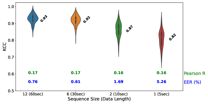
Figure 1: KCC violin plots for different data lengths with GazeBase dataset. Sequence size - Data length is on the x-axis. A sequence is of 5000 time steps. The KCC is plotted on the y-axis, and Intercorrelation (Pearson R) and EER are annotated on the plot in green and blue respectively.

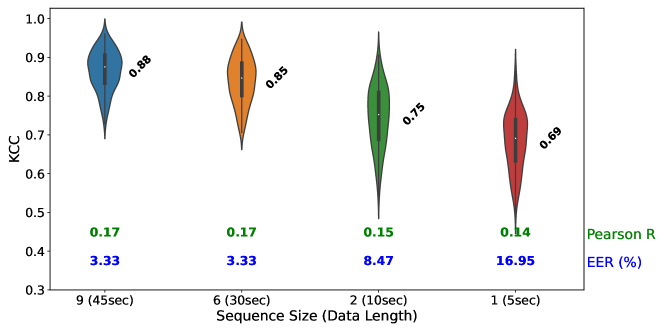
Figure 2: KCC violin plots for different data lengths with GazeBaseVR dataset. Sequence size - Data length is on the x-axis. KCC is plotted on the y-axis. The annotation on the plot is same as Fig. 1.

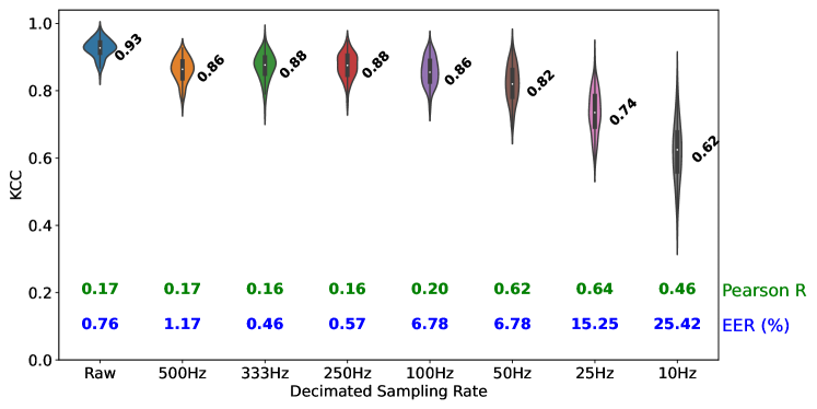
Figure 3: KCC violin plots for decimated sampling rates using GazeBase dataset. Decimated Sampling Rate levels are presented on the x-axis. KCC is plotted on the y-axis. The annotation on the plot is same as Fig. 1.

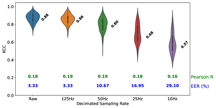
Figure 4: KCC violin plots for decimated sampling rates using GazeBaseVR dataset. Decimated Sampling Rate levels are presented on the x-axis. KCC is plotted on the y-axis. The annotation on the plot is same as Fig. 1.

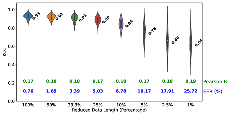
Figure 5: KCC violin plots using various percentages of each recording of the GazeBase dataset. Reduced data length in percentage is on the x-axis. KCC is plotted on the y-axis. The annotation on the plot is same as Fig. 1.

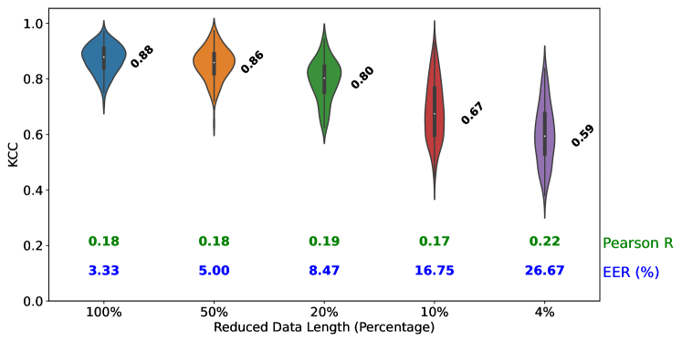
Figure 6: KCC violin plots using various percentages of each recording of the GazeBaseVR dataset. Reduced data length in percentage is on the x-axis. KCC is plotted on the y-axis. The annotation on the plot is same as Fig. 1.

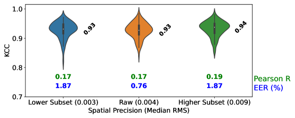
Figure 7: KCC violin plots comparison between higher spatial precision data subset and lower spatial precision data subset of the GazeBase dataset. The median RMS of different levels is on the x-axis. KCC is plotted on the y-axis. The annotation on the plot is same as Fig. 1.

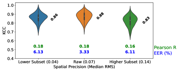
Figure 8: KCC violin plots comparison between higher spatial precision data subset and lower spatial precision data subset of the GazeBaseVR dataset. The median RMS of different levels is on the x-axis. KCC is plotted on the y-axis. The annotation on the plot is same as Fig. 1.

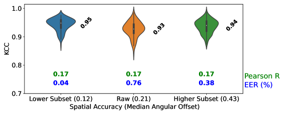
Figure 9: KCC violin plots comparison between higher spatial accuracy data subset and lower spatial accuracy data subset of the GazeBase dataset. The median angular offset of different levels is on the x-axis. KCC is plotted on the y-axis. The annotation on the plot is same as Fig. 1.

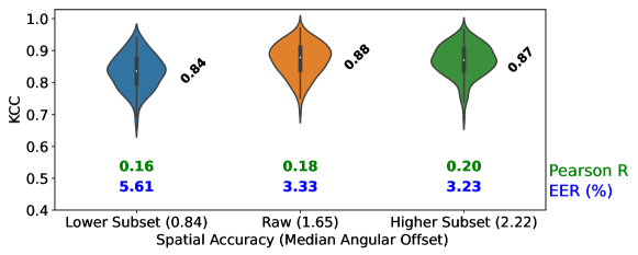
Figure 10: KCC violin plots comparison between higher spatial accuracy data subset and lower spatial accuracy data subset of the GazeBaseVR dataset. The median angular offset of different levels is on the x-axis. KCC is plotted on the y-axis. The annotation on the plot is same as Fig. 1.

5.1 Effect on Embedding Calculated Over various Sequence sizes

We have demonstrated the effect of embedding calculated over various sequence sizes in Fig. 1, 2 in terms of KCC, Pearson R, and EER.

The blue, orange, green, and red violins represent the distribution of KCC values at different data lengths. The values above each violin represent the median KCC value for that data length. KCC values are between 0 and 1, with 1 indicating perfect agreement among raters.

For the GazeBase dataset, KCC is notably high for 12 sequences of a 5-second window, totaling 60 seconds of analyzed data. A decline in KCC values is observed as the data length is reduced, indicating a decrease in raters’ agreement and suggesting less stability in the embedding with shorter lengths. Despite this, the median KCC values remain high (above 0.8), indicating a consistent strong agreement among raters for various data lengths. The Equal Error Rate (EER) percentages, marked in blue on the plot, reveal an increase in EER as the data length shortens from 60 seconds to 5 seconds, implying a degradation in biometric performance with reduced data lengths except for 30 seconds data length. The EER at 60 seconds stands at a low 0.61%, indicating strong performance, whereas at 5 seconds, it rises to 3.51%, highlighting a significant decline in biometric performance. In short, the graph illustrates an increase in EER for embeddings generated from shorter data lengths compared to those derived from longer segments. The Pearson correlation coefficient remains nearly unchanged across different data lengths.

A similar pattern is observed in the GazeBaseVR dataset, as depicted in Fig. 2. Here, KCC is high for 9 sequences of a 5-second window, equating to 45 seconds of data. The reduction in data length leads to a downward trend in KCC values for GazeBaseVR as well. The trend of increasing EER with decreasing data length is also evident in this dataset, indicating a decrease in biometric performance with shorter data spans. Thus, the plot for the GazeBaseVR dataset similarly demonstrates higher EER for embeddings calculated from shorter data lengths, with the Pearson correlation coefficient maintaining consistency across various data lengths with a slightly downward trend.

5.2 Effect of Sampling Rate

In Fig. 3, 4, the x-axis of the plot shows different sampling rates, from ‘Raw’ to ‘10Hz’ for GazeBase and GazeBaseVR datasets respectively. ‘Raw’ indicates the original sampling rate without decimation. The other labels (500Hz, 333Hz, 250Hz, etc.) suggest that the original signal has been decimated to these lower rates. Each violin plot corresponds to a different sampling rate, with the width of each plot representing the density of the KCC values at that sampling rate. Within each violin plot, the number indicates the median KCC value. Below the x-axis, the blue and green numbers correspond to the Pearson R and EER, respectively, at each decimated level.

In Fig. 3, the KCC starts high at ‘Raw’ and decreases slightly but remains relatively stable until the sampling rate is decreased to 50 Hz, beyond which there is a marked decrease. The Pearson R remains relatively consistent until 250 Hz and then we see a rise in the Pearson R among the lower sampling rates, without following a particular trend. The EER starts low at ‘Raw’ but lowest at 333 Hz (0.46) and increases with each step of decimation after that, indicating that the error rate increases as the sampling rate decreases. The result suggests that intercorrelation (as measured by Pearson R) increases as the sampling rate is reduced, while the KCC decreases and the error rate increases, particularly at lower sampling rates. It means that embeddings can tolerate some reduction in sampling rate without significant loss of reliability up to a point, after which the reliability decreases significantly.

A similar pattern is observed in the GazeBaseVR dataset, as depicted in Fig. 4. In the GazeBaseVR dataset, a high median KCC is observed at the ‘Raw’ sampling rate (0.88). As the sampling rate decreases, the KCC values exhibit a gradual decline, mirroring the trend seen in the GazeBase dataset. This decline becomes more pronounced at lower sampling rates, indicating a loss in temporal persistence as the data’s temporal resolution diminishes. The Pearson R values in the GazeBaseVR dataset maintain a remarkable consistency across all levels of decimation, unlike the GazeBase dataset. However, the EER metric tells a different story. Starting from a low baseline at the ‘Raw’ sampling rate, the EER steadily increases with each reduction in sampling rate after 125Hz. This upward trend in EER highlights a growing disparity in the biometric performance of the dataset, where lower sampling rates correlate with higher error rates.

5.3 Effect of Reduced Sample Length during Training

In Fig. 5, the colored violins represent the distribution of KCC values using various percentages of data in the training process with GazeBase dataset. At 100% data length, the KCC is quite high (median-0.93), and the Pearson R is low (0.17), with a very low EER (0.76%). This suggests strong agreement and low error with the full data. As data is reduced, KCC starts to decline and reaches 0.64 for 1% of data. The Pearson R values in the GazeBase dataset maintain a remarkable consistency across all levels. The EER increases as the data is reduced, suggesting a rise in error rate with less data.

Turning to Figure 6, which explores the GazeBaseVR dataset, a similar pattern emerges. The KCC values commence a descent as the dataset is progressively reduced, reaching a median of 0.59 at just 4% of the data. This decline mirrors the trend observed in the GazeBase dataset, highlighting a loss in agreement with decreasing data sizes. Similar to the GazeBase dataset, the Pearson R values in the GazeBaseVR analysis exhibit remarkable stability across all data percentages with a slight upward trend, suggesting that the linear correlation among variables remains unaffected by the reduction in data size. The EER rises as less data is utilized, reinforcing the correlation between reduced dataset sizes and increased error rates in biometric authentication processes.

5.4 Effect of Eye Tracking Signal Quality

5.4.1 Comparison in terms of Precision

In Fig. 7, ‘KCC’ is labeled in y-axis, ranges from 0.7 to 1.0, indicating that all KCC values are relatively high, which implies generally higher reliability across all precision levels. The lower Subset is the subset of the raw data with the lowest median RMS value and the higher subset is the highest median RMS. KCC is very high and stable for all three levels of comparison (Lower RMS subset vs Raw data vs Higher RMS subset). In short, negligible differences can be seen in terms of KCC. The Pearson correlation coefficients, annotated on the plot in green, also remain stable despite being in the smaller range between 0.16 to 0.19. The EER percentages at the bottom of the plot indicate that as precision changes, the equal error rate increases. Overall, the plot shows that while precision does have a negligible impact on the KCC and intercorrelation but affects biometric performance.

Exactly similar pattern is seen in Fig. 8 where we used the GazeBaseVR dataset.

5.4.2 Comparison in terms of Spatial Accuracy

In Fig. 9 y-axis, labeled ‘KCC’, all above 0.9, indicating that there is no change in the KCC median values, which indicates stable reliability. The Pearson correlation coefficients, annotated on the plot in green, suggest a relationship with the accuracy of the data. The EER percentages at the bottom of the plot indicate that as accuracy drops, the equal error rate increases. Best EER is achieved with lower-angular-offset-subset for GazeBase. Overall, the plot shows that any change in the accuracy does not impact the KCC calculated on the embeddings and intercorrelation.

Fig. 10 where we used the GazeBaseVR dataset shows a different trend in terms of EER. Interestingly, the higher-angular-offset-subset outperforms both the lower subset and raw data in terms of EER. Pearson R increases with the increase in median angular offset.

6 Discussion

Table 1 shows the effect of input data variability on embeddings in terms of performance metrics. The key facts of the paper are discussed in the following subsections:

Table 1: Impact on Embeddings: Performance Metrics Variation. Symbols: $\times$ indicates a significant effect due to input variability; - denotes negligible impact.

Experiments	KCC	Pearson R	EER
Various Sequence sizes	$\times$	-	$\times$
Reducing Sampling rate (Decimation)	$\times$	$\times$	$\times$
Reduced data length during training (Percentage)	$\times$	-	$\times$
Spatial Precision based analysis	-	-	$\times$
Spatial Accuracy based analysis	-	-	$\times$

6.1 Summary of Findings

1. We found that varying sequence sizes significantly influenced the embeddings. Longer sequences generally resulted in more reliable and consistent embeddings, as evidenced by higher Kendall’s Coefficient of Concordance (KCC) values for 12 consecutive sequences (60 seconds) compared to 1 sequence (5 seconds) of data. However, there was a diminishing return on increasing data length beyond a certain point. The most significant impact was observed when comparing very short data sequences to moderately long ones. The improvement in embedding reliability was marked, as evidenced by a noticeable shift in key metrics. A significant drop in biometric performance in terms of Equal Error Rate (EER) is also seen in the results.

2. 1. The impact of different sampling rates on embeddings was profound. Our experiments showed that while embeddings maintained a degree of stability up to moderate reductions in sampling rate (as indicated by stable KCC and Pearson R values), further reduction led to a noticeable decrease in reliability and an increase in EER. This suggests that while some degree of decimation is tolerable, excessively low sampling rates compromise the efficacy of the biometric system by a heavy margin. A critical point was identified where further reduction in the rate led to a disproportionate decrease in the quality of embeddings. This threshold point was a key finding, indicating the minimum viable sampling rate for effective biometric authentication.

   2. We also found that reduced data length from the recording during taing process significantly influenced the embeddings. Lowering the given data percentages resulted in less reliable embeddings, as evidenced by a downward trend of KCC from 100% to 1 % of data. A significant drop in biometric performance in terms of Equal Error Rate (EER) is also seen in the results.

3. The study also delved into how eye-tracking signal quality affects embeddings. We distinguished between spatial precision and spatial accuracy, noting their influence on the KCC, intercorrelations, and EER of the embeddings. Results indicated that while there was a slight decrease in KCC with reduced signal quality, the overall impact was not as significant as might be expected.

6.2 Methodological Strengths & Limitations

The Eye Know You Too (EKYT) network architecture was chosen for our study due to its state-of-the-art performance in biometric authentication, particularly with high-quality data. The EKYT architecture is based on a DenseNet framework, which is known for its efficiency in handling complex data structures. The EKYT model is specifically optimized for high-quality data (like data collected at 1000 Hz), making it suitable for the datasets used in our study. This ensures that the model can leverage the detailed information available in high-quality eye movement data for better authentication performance. The output of the EKYT is a 128-dimensional embedding of the eye-tracking signal given as the input sequence. These embeddings are critical for biometric authentication as they represent a compact and informative representation of the original eye movement data.

Our research involved 322 participants in Round 1 and 59 in Round 6, with the latter being a subset of the former. This may still be limited for capturing the full variability in a general population. However, this size is reasonably large from the eye-tracking research perspective. The limited dataset size can impact the scalability of the findings. For instance, the system’s performance might vary when exposed to a more diverse and larger population, where new and unforeseen patterns of eye movements could emerge. The reader should keep this in mind.

6.3 Future Research Direction

This research highlights crucial future research directions, particularly in understanding the significance of the embeddings learned through deep learning in biometric authentication. A key focus should be on enhancing these embeddings to improve the temporal persistence of the EMB system, while simultaneously maintaining its biometric performance. This should involve exploring methods to optimize the learning process within the deep learning pipeline, ensuring that the reliability and accuracy of the biometric system are not compromised.

7 Conclusion

In this paper, we aimed to explore if the embeddings learned from machine learning pipeline exhibit the same level of temporal stability as seen in traditional biometric features in eye movement biometrics. Our study also focused on the influence of varying input data on the persistence, and reliability of embeddings and stability and consistency of the biometric performance in the context of eye movement biometrics. Additionally, our research sought to understand the relationship between the variability of eye-tracking signal quality and the overall reliability of eye movement biometric system. We have utilized the state-of-the-art EKYT architecture in this paper and designed multiple experiments with the above goal in mind. All of the three metrics (KCC, Pearson R, and EER) provide us with a clear indication of how conducting various analyses impacts the learned embeddings. The results suggest that reliability is directly related to the data length and data sampling rate. Any variation in the data length in any manner affects the learned embeddings from the temporal persistence and biometric efficacy perspective. Intercorrelations do not vary much throughout the conducted research. To summarize, our study not only validates the relevance of the temporal persistence of embeddings to the biometric authentication system but also underscores minimal variations in intercorrelations, consistent with our initial hypotheses.

References

- [1] R. Alrawili, A. A. S. AlQahtani, and M. K. Khan, “Comprehensive survey: Biometric user authentication application, evaluation, and discussion,” arXiv preprint arXiv:2311.13416, 2023.
- [2] L. Friedman, M. S. Nixon, and O. V. Komogortsev, “Method to assess the temporal persistence of potential biometric features: Application to oculomotor, gait, face and brain structure databases,” PLOS ONE, vol. 12, no. 6, pp. 1–42, 06 2017. [Online]. Available: https://doi.org/10.1371/journal.pone.0178501
- [3] L. Friedman, H. S. Stern, L. R. Price, and O. V. Komogortsev, “Why temporal persistence of biometric features, as assessed by the intraclass correlation coefficient, is so valuable for classification performance,” Sensors, vol. 20, no. 16, p. 4555, 2020.
- [4] P. Kasprowski and J. Ober, “Eye movements in biometrics,” Lecture Notes in Computer Science (including subseries Lecture Notes in Artificial Intelligence and Lecture Notes in Bioinformatics), vol. 3087, pp. 248–258, 2004. [Online]. Available: https://doi.org/10.1007/978-3-540-25976-3_23
- [5] C. Katsini, Y. Abdrabou, G. E. Raptis, M. Khamis, and F. Alt, “The Role of Eye Gaze in Security and Privacy Applications: Survey and Future HCI Research Directions,” in Proceedings of the 2020 CHI Conference on Human Factors in Computing Systems, ser. CHI ’20. Honolulu, HI, USA: Association for Computing Machinery, Apr. 2020, pp. 1–21. [Online]. Available: https://doi.org/10.1145/3313831.3376840
- [6] G. Bargary, J. M. Bosten, P. T. Goodbourn, A. J. Lawrance-Owen, R. E. Hogg, and J. D. Mollon, “Individual differences in human eye movements: An oculomotor signature?” Vision Research, vol. 141, pp. 157–169, Dec. 2017. [Online]. Available: http://www.sciencedirect.com/science/article/pii/S0042698917300391
- [7] M. Nilsson Benfatto, G. Öqvist Seimyr, J. Ygge, T. Pansell, A. Rydberg, and C. Jacobson, “Screening for dyslexia using eye tracking during reading,” PloS one, vol. 11, no. 12, p. e0165508, 2016.
- [8] L. Billeci, A. Narzisi, A. Tonacci, B. Sbriscia-Fioretti, L. Serasini, F. Fulceri, F. Apicella, F. Sicca, S. Calderoni, and F. Muratori, “An integrated eeg and eye-tracking approach for the study of responding and initiating joint attention in autism spectrum disorders,” Scientific Reports, vol. 7, no. 1, p. 13560, 2017.
- [9] B. A. Sargezeh, N. Tavakoli, and M. R. Daliri, “Gender-based eye movement differences in passive indoor picture viewing: An eye-tracking study,” Physiology & behavior, vol. 206, pp. 43–50, 2019.
- [10] S. M. K. Al Zaidawi, M. H. Prinzler, C. Schröder, G. Zachmann, and S. Maneth, “Gender classification of prepubescent children via eye movements with reading stimuli,” in Companion Publication of the 2020 International Conference on Multimodal Interaction, 2020, pp. 1–6.
- [11] C. Schröder, S. M. K. Al Zaidawi, M. H. Prinzler, S. Maneth, and G. Zachmann, “Robustness of eye movement biometrics against varying stimuli and varying trajectory length,” in Proceedings of the 2020 CHI Conference on Human Factors in Computing Systems, 2020, pp. 1–7.
- [12] I. Rigas and O. V. Komogortsev, “Current research in eye movement biometrics: An analysis based on bioeye 2015 competition,” Image and Vision Computing, vol. 58, pp. 129–141, 2017.
- [13] S. Eberz, K. Rasmussen, V. Lenders, and I. Martinovic, “Preventing lunchtime attacks: Fighting insider threats with eye movement biometrics,” in Network and Distributed System Security (NDSS) Symposium. Internet Society, 2015. [Online]. Available: http://dx.doi.org/10.14722/ndss.2015.23203
- [14] O. V. Komogortsev, A. Karpov, and C. D. Holland, “Attack of mechanical replicas: Liveness detection with eye movements,” IEEE Transactions on Information Forensics and Security, vol. 10, no. 4, pp. 716–725, 2015. [Online]. Available: https://doi.org/10.1109/TIFS.2015.2405345
- [15] I. Rigas and O. V. Komogortsev, “Eye Movement-Driven Defense against Iris Print-Attacks,” Pattern Recogn. Lett., vol. 68, no. P2, p. 316–326, dec 2015. [Online]. Available: http://dx.doi.org/10.1016/j.patrec.2015.06.011
- [16] M. H. Raju, D. J. Lohr, and O. Komogortsev, “Iris print attack detection using eye movement signals,” in 2022 Symposium on Eye Tracking Research and Applications, ser. ETRA ’22. New York, NY, USA: Association for Computing Machinery, 2022. [Online]. Available: https://doi.org/10.1145/3517031.3532521
- [17] D. Lohr, H. Griffith, S. Aziz, and O. Komogortsev, “A metric learning approach to eye movement biometrics,” in 2020 IEEE International Joint Conference on Biometrics (IJCB). IEEE, 2020, pp. 1–7. [Online]. Available: http://dx.doi.org/10.1109/IJCB48548.2020.9304859
- [18] D. J. Lohr, S. Aziz, and O. Komogortsev, “Eye movement biometrics using a new dataset collected in virtual reality,” in ACM Symposium on Eye Tracking Research and Applications, ser. ETRA ’20 Adjunct. New York, NY, USA: Association for Computing Machinery, 2020. [Online]. Available: https://doi.org/10.1145/3379157.3391420
- [19] D. Lohr, H. Griffith, and O. V. Komogortsev, “Eye know you: Metric learning for end-to-end biometric authentication using eye movements from a longitudinal dataset,” IEEE Transactions on Biometrics, Behavior, and Identity Science, 2022.
- [20] L. A. Jäger, S. Makowski, P. Prasse, S. Liehr, M. Seidler, and T. Scheffer, “Deep eyedentification: Biometric identification using micro-movements of the eye,” in Machine Learning and Knowledge Discovery in Databases: European Conference, ECML PKDD 2019, Würzburg, Germany, September 16–20, 2019, Proceedings, Part II. Springer, 2020, pp. 299–314.
- [21] S. Makowski, P. Prasse, D. R. Reich, D. Krakowczyk, L. A. Jäger, and T. Scheffer, “Deepeyedentificationlive: Oculomotoric biometric identification and presentation-attack detection using deep neural networks,” IEEE Transactions on Biometrics, Behavior, and Identity Science, vol. 3, no. 4, pp. 506–518, 2021.
- [22] D. Lohr and O. V. Komogortsev, “Eye know you too: Toward viable end-to-end eye movement biometrics for user authentication,” IEEE Transactions on Information Forensics and Security, vol. 17, pp. 3151–3164, 2022.
- [23] A. R. A. Brasil, J. O. Andrade, and K. S. Komati, “Eye movements biometrics: A bibliometric analysis from 2004 to 2019,” arXiv preprint arXiv:2006.01310, 2020.
- [24] Y. Zhang and X. Mou, “Survey on eye movement based authentication systems,” in Computer Vision: CCF Chinese Conference, CCCV 2015, Xi’an, China, September 18-20, 2015, Proceedings, Part I. Springer, 2015, pp. 144–159.
- [25] Y. Zhang and M. Juhola, “On biometrics with eye movements,” IEEE journal of biomedical and health informatics, vol. 21, no. 5, pp. 1360–1366, 2016.
- [26] I. Rigas and O. V. Komogortsev, “Current research in eye movement biometrics: An analysis based on BioEye 2015 competition,” Image and Vision Computing, vol. 58, pp. 129–141, 2017.
- [27] R. Andersson, L. Larsson, K. Holmqvist, M. Stridh, and M. Nyström, “One algorithm to rule them all? An evaluation and discussion of ten eye movement event-detection algorithms,” Behavior Research Methods, vol. 49, no. 2, pp. 616–637, 2017. [Online]. Available: https://doi.org/10.3758/s13428-016-0738-9
- [28] M. Nyström and K. Holmqvist, “An adaptive algorithm for fixation, saccade, and glissade detection in eyetracking data,” Behavior research methods, vol. 42, no. 1, pp. 188–204, 2010.
- [29] J. Pekkanen and O. Lappi, “A new and general approach to signal denoising and eye movement classification based on segmented linear regression,” Scientific reports, vol. 7, no. 1, p. 17726, 2017.
- [30] A. H. Dar, A. S. Wagner, and M. Hanke, “Remodnav: robust eye-movement classification for dynamic stimulation,” Behavior research methods, vol. 53, no. 1, pp. 399–414, 2021.
- [31] L. Friedman, I. Rigas, E. Abdulin, and O. V. Komogortsev, “A novel evaluation of two related and two independent algorithms for eye movement classification during reading,” Behavior Research Methods, vol. 50, no. 4, pp. 1374–1397, 08 2018. [Online]. Available: https://doi.org/10.3758/s13428-018-1050-7
- [32] C. Li, J. Xue, C. Quan, J. Yue, and C. Zhang, “Biometric recognition via texture features of eye movement trajectories in a visual searching task,” PLoS ONE, vol. 13, no. 4, p. e0194475, apr 2018. [Online]. Available: https://dx.plos.org/10.1371/journal.pone.0194475
- [33] I. Rigas, G. Economou, and S. Fotopoulos, “Biometric identification based on the eye movements and graph matching techniques,” Pattern Recognition Letters, vol. 33, no. 6, pp. 786–792, 2012.
- [34] I. Rigas, O. Komogortsev, and R. Shadmehr, “Biometric recognition via eye movements: Saccadic vigor and acceleration cues,” ACM Transactions on Applied Perception (TAP), vol. 13, no. 2, pp. 1–21, 2016.
- [35] C. D. Holland and O. V. Komogortsev, “Complex eye movement pattern biometrics: Analyzing fixations and saccades,” in 2013 International conference on biometrics (ICB). IEEE, 2013, pp. 1–8.
- [36] A. George and A. Routray, “A score level fusion method for eye movement biometrics,” Pattern Recognition Letters, vol. 82, pp. 207–215, 2016.
- [37] S. Jia, D. H. Koh, A. Seccia, P. Antonenko, R. Lamb, A. Keil, M. Schneps, and M. Pomplun, “Biometric recognition through eye movements using a recurrent neural network,” in Proceedings - 9th IEEE International Conference on Big Knowledge, ICBK 2018. Institute of Electrical and Electronics Engineers Inc., dec 2018, pp. 57–64.
- [38] A. Abdelwahab and N. Landwehr, “Deep distributional sequence embeddings based on a wasserstein loss,” Neural Processing Letters, vol. 54, no. 5, pp. 3749–3769, 2022.
- [39] H. Griffith, D. Lohr, E. Abdulin, and O. Komogortsev, “Gazebase, a large-scale, multi-stimulus, longitudinal eye movement dataset,” Scientific Data, vol. 8, no. 1, p. 184, 2021.
- [40] D. Lohr, S. Aziz, L. Friedman, and O. V. Komogortsev, “Gazebasevr, a large-scale, longitudinal, binocular eye-tracking dataset collected in virtual reality,” Scientific Data, vol. 10, no. 1, 2023.
- [41] A. Savitzky and M. J. Golay, “Smoothing and differentiation of data by simplified least squares procedures.” Analytical chemistry, vol. 36, no. 8, pp. 1627–1639, 1964.
- [42] G. Huang, Z. Liu, L. Van Der Maaten, and K. Q. Weinberger, “Densely connected convolutional networks,” in Proceedings of the IEEE conference on computer vision and pattern recognition, 2017, pp. 4700–4708.
- [43] D. P. Kingma and J. Ba, “Adam: A method for stochastic optimization,” arXiv preprint arXiv:1412.6980, 2014.
- [44] L. N. Smith and N. Topin, “Super-convergence: Very fast training of neural networks using large learning rates,” in Artificial intelligence and machine learning for multi-domain operations applications, vol. 11006. SPIE, 2019, pp. 369–386.
- [45] X. Wang, X. Han, W. Huang, D. Dong, and M. R. Scott, “Multi-similarity loss with general pair weighting for deep metric learning,” in 2019 IEEE/CVF Conference on Computer Vision and Pattern Recognition (CVPR), 2019, pp. 5017–5025.
- [46] A. P. Field, “Kendall’s coefficient of concordance,” Encyclopedia of Statistics in Behavioral Science, vol. 2, pp. 1010–11, 2005.
- [47] K. Musgrave, S. Belongie, and S.-N. Lim, “Pytorch metric learning,” 2020.
- [48] D. J. Lohr, L. Friedman, and O. V. Komogortsev, “Evaluating the data quality of eye tracking signals from a virtual reality system: Case study using smi’s eye-tracking htc vive,” arXiv preprint arXiv:1912.02083, 2019.