Information Theory Unification
of
Epidemiological and Population Dynamics
Abstract
We reformulate models in epidemiology and population dynamics in terms of probability distributions. This allows us to construct the Fisher information, which we interpret as the metric of a one-dimensional differentiable manifold. For systems that can be effectively described by a single degree of freedom, we show that their time evolution is fully captured by this metric. In this way, we discover universal features across seemingly very different models. This further motivates a reorganisation of the dynamics around zeroes of the Fisher metric, corresponding to extrema of the probability distribution. Concretely, we propose a simple form of the metric for which we can analytically solve the dynamics of the system that well approximates the time evolution of various established models in epidemiology and population dynamics, thus providing a unifying framework.
11footnotemark: 122footnotemark: 2 Univ Lyon, Univ Claude Bernard Lyon 1, CNRS/IN2P3, IP2I Lyon, UMR 5822, F-69622, Villeurbanne, France
22footnotemark: 233footnotemark: 3 Dept. of Physics E. Pancini, Università di Napoli Federico II, via Cintia, 80126 Napoli, Italy
33footnotemark: 3 INFN sezione di Napoli, via Cintia, 80126 Napoli, Italy
33footnotemark: 3 Quantum Theory Center (QTC) & D-IAS, Southern Denmark Univ., Campusvej 55, 5230 Odense M, Denmark
1 Introduction
Describing the probabilities for a discrete set of events to happen, is an important question, both in mathematics and physics. In most cases, these probabilities depend on a number of discrete or continuous parameters, related to the system under consideration. Capturing these dependences in an efficient manner is for example the basis for optimisation strategies and therefore the foundation for many practical applications. The field of information geometry, as part of information theory, proposes to describe probability distributions in a geometric fashion. Indeed, in the pioneering works [1, 2, 3, 4], the question how to quantify the difference of two sets of probabilities as a function of external parameters, has been approached using geometric tools: concretely, a Riemannian manifold has been introduced, which is equipped with a metric (called the Fisher information metric) and a geodesic distance (called the Fisher-Rao distance). These works have further been generalised in [5, 6, 7, 8, 9, 10] by adding additional structure to the manifold, such as conjugate pairs of connections and higher order tensors, leading to a more refined geometric realisation and description of probability distributions.
In this paper, we propose to apply the ideas of information theory to (at least partially) describe and in fact capture the time evolution of simple systems that are relevant for population dynamics and epidemiology. The models under consideration group a given population (of potentially variable size) into different classes, e.g. ’predator’ and ’prey’ (in the case of the Lotka-Volterra model [11, 12]) or ’susceptible’ and ’infectious’ (in the case of the epidemiological SI-model [13]). The dynamics of each system is captured by describing the size of these classes as a function of time , which is encoded in a set of coupled, non-linear, first-order differential equations, supplemented by suitable initial conditions. Within this framework, we can naturally444In fact, in many examples, we can study different probability distributions, which exhibit different aspects of the system under consideration. define a probability distribution (for ) as a set of normalised (i.e. such that ) fractions of these classes within the population. Following [1, 2, 3], we can construct a 1-dimensional differentiable manifold that represents the time-dependence of these probabilities. This manifold is concretely given through the Fisher information metric , which is a non-negative, differentiable function of time.555Following the original definition in [1], is often simply called Fisher information. Although here it is the metric for ’only’ a 1-dimensional manifold, in the following we shall continue to refer to it as ’Fisher (information) metric’ (or simply ’metric’ for short) to highlight its property to provide a notion of ’distance’ between probability distributions at different times, which is its essential property for our discussion.
Notice that the Fisher metric is a priori calculated from the time-dependence of the probability distribution, which itself is determined by other means. In this paper we are interested in the inverse problem, i.e. to fix the time evolution of the probability distribution from the metric , which serves as input for the dynamics. We first argue that under certain conditions, the time dependence of the system can in fact be fully described in terms of the Fisher metric: indeed, in cases where only two of the probabilities vary strongly with time, while the remaining ones remain approximately static (such that the full time evolution can be encoded in a single, bounded function for ), we can re-write the equation of motion for the dynamical probabilities completely in terms of the Fisher metric . Such a scenario is trivially realised in models with , which is the case of the Lotka-Volterra or SI-model. We also provide further, more sophisticated, examples in which such a scenario can be realised, namely compartmental models in epidemiology (see [14, 15, 16, 17, 18, 19, 20] for reviews), particularly with multiple competing variants of a pathogen (see e.g. [21]).
An important step for the metric to capture the full dynamics of the system is to re-write as a function of rather than a(n explicit) function of . For the examples mentioned above, this requires partially solving the original equations of motion and in particular to incorporate the initial conditions of the problem. In the case of the Lotka-Volterra model, the SIR model and a simple compartmental model with competing variants, we manage to perform this step analytically and write a closed form expression of the metric as a function of . For further examples, we provide numerical solutions that allow to study the re-organisations of the time evolution in terms of the metric. Comparing the specific form of obtained in this way, we find strong similarities among a priori very different systems, which can be summarised as follows:
-
(i)
real zeroes of the metric correspond to extrema of the probability
-
(ii)
the metric can be described piecewise between two consecutive extrema of the probability (, such that ),i.e. in regimes where is a monotonic function
-
•
in the simplest case, the metric is a convex function and can be very well approximated in a simple form , where are suitable fitting coefficients (with the powers of order )
-
•
the metric can have local minima, in which case it can be well approximated to include factors with complex zeroes, e.g. with (and ) and
-
•
-
(iii)
by gluing together branches of the metric along their (real) zeroes, non-monotonic behaviour of the probability can be described, notably periodic and oscillating solutions as in the case of the Lotka-Volterra model and the SIR-model respectively.
Motivated by these common properties of different types of systems, we propose a universal description of the dynamics of the probability distribution, which uses the metric as external input (supplemented by suitable initial conditions): the monotonic evolution of can be described by a metric that is proportional to (products of) monomials of its zeroes. For the simplest choice as the product of two simple, real zeroes at , we provide an analytic, closed form solution for the monotonic time evolution of from its initial value to one of its extrema at . By gluing metrics of this form together, we can describe explicitly more general solutions, notably periodic or oscillating types, which are capable of approximating the dynamics of more complicated systems. Due to the universality of our approach, it can be used to model various different phenomena in a common form thereby unifying them within the information theory framework.
This paper is organised as follows: in Section 2 we review important aspects of Information Theory, defining notably the Fisher information metric. In Section 3 we study simple theoretical models (i.e. the Lotka-Volterra model and the SIR model as well as generalisations thereof that allow for multiple variants of a disease to spread among the population): we calculate their Fisher information metric and re-write it in terms of the probability distribution, thereby uncovering its universal features. In Section 4 we provide an analytic solution of the time evolution of a monotonic probability distribution provided that a simple metric is given as input. Based on this, we can describe more complicated behaviours by gluing together solutions of this form, thereby providing a simple approximation to the systems studied in Section 3. Finally, Section 5 contains our conclusions.
2 Review of Information Theory
In this Section we introduce and review a number of mathematical tools that are aimed at quantifying the ’unevenness’ [22] in a probability distribution and its characterisation in geometric terms. We follow, in particular, the Riemannian approach advocated in [1, 2, 3, 4] and further generalised in [5, 6].
2.1 Information Geometry
Let be a discrete set and define a probability distribution as a map [23, 6]
| such that | (2.1) |
Given two such distributions and on the same set , their ’difference’ can be captured by various divergences [24, 25] (see also [7, 6, 22, 26]), e.g. the Kullback-Leibler divergence [27]666In information theoretical works, the base of the logarithm is usually chosen to be 2. In this paper we shall use the natural logarithm with base .
| (2.2) |
which is non-negative () and vanishes only if the probability distributions are identical. However, it is not symmetric (i.e. in general ) and also does not satisfy the triangle inequality and therefore does not constitute a distance function, which makes a geometric interpretation difficult.
To remedy this, we shall follow the initial work of [1, 2, 3, 4, 28] to provide a Riemann geometric interpretation of (families of) probability distributions, which was further extended in [5, 6, 7] (see also [8, 9, 10]). To this end, we first generalise the definition (2.1) by allowing to depend on a number of (continuous) parameters. Let (which we assume to be an open subset of ) with (and ) and consider the probability distributions
| with | (2.3) |
which we assume to be (infinitely continuously) differentiable with respect to .777We shall also implicitly assume that the derivatives commute with integration. Following [6], we furthermore call a family of probability distributions
| (2.4) |
such that is injective , a statistical model. It was shown in [6] that can be endowed with the structure of a differentiable manifold (also called statistical manifold) and equipped with a Riemannian metric, called the Fisher information metric888When simply viewed as a matrix, this quantity is also called the Fisher information matrix or in the case simply the Fisher information. [3, 4, 28, 6, 26]
| (2.5) |
For a given , this metric can be used to define a distance between two probability distributions [3, 4] (see also [26, 29]): let be a curve in (parametrised by ). Such a curve is a geodesic if it satisfies
| with | (2.8) |
where is the inverse of the metric (2.5). We can then define the Fisher-Rao distance of the probability distributions and for as
| (2.9) |
where is the geodesic such that and .
2.2 Time Evolution and Flow Equations
In this paper, we shall exclusively be interested in the one-dimensional case , where we shall interpret as a time variable. In this case, we use the following notation for the one-dimensional metric (following from the general definition (2.5)).
| with | (2.10) |
with an infinitesimal time element.999As remarked before, is the Fisher information, originally introduced in [1]. In the following, to highlight its property to keep track of changes or differences of , we shall refer to it as ’Fisher (information) metric’ (or simply ’metric’ for short). We first remark that the metric element can in fact be related to the Kullback-Leibler divergence (2.2) of and (see [22]))
| (2.11) |
Furthermore, the Fisher-Rao distance (2.9) becomes the (absolute value) of the proper time
| (2.12) |
Moreover, we shall argue that (2.10) can be used to describe the time evolution of the probability distribution , at least in certain cases. To this end, we focus on a finite set of cardinality and define the probability distribution
| with | ||||||
| (2.13) | ||||||
We resolve the normalisation condition by defining (with ), such that
| and | (2.14) |
The Fisher information metric (2.10) can then be written as (with )
| (2.15) |
Rather than calculating the metric for a (given) probability distribution, we shall in the following try to extract information about in terms of the metric , taking the latter as an input. In general, it is not possible to extract the time evolution for all in this manner, however, by making further assumptions on the form of the dynamics, we can derive certain insights. As an example, consider the case in which one of the probabilities is very close to zero, e.g. without loss of generality . In this case, the metric (2.15) is dominated by a single term
| such that | (2.16) |
The sign in the last equation cannot be uniquely fixed due to time inversion symmetry and is determined whether the probability is growing or diminishing. Notice, that (2.16) is an effective description of the time evolution of , where the entire dynamics of the rest of the system (i.e. ) is encoded in the metric .
In the remainder of this paper, we shall study in detail a different scenario than (2.16): consider the case where the time derivative of one probability is much larger than the others101010From the perspective of the , the condition (2.17) implies that grows (diminishes) at the expense of , while the remaining probabilities remain essentially constant. This scenario therefore corresponds to a competition between two probabilities, which can both take values in the interval ., thus, without loss of generality
| such that | (2.17) |
In this case, the metric can be approximated by
| (2.18) |
This equation can be re-written in the following fashion
| with | (2.19) |
where the sign cannot be fixed and is determined by whether the probability is growing or diminishing. If is considered as an (external) input, equation (2.19) can be understood as an effective description of the dynamics for . In particular, in the case that is given as a function of (thereby encoding the influence of the remainder of the system on ), (2.19) uniquely fixes the time evolution of . In this case, (2.19) plays a similar role to the flow equations in epidemiology discussed in [21]. Notice in this respect that and denote the extremal values can take.
We furthermore remark, that in the particular case (2.17) the dynamics of can in fact be solved in terms of the proper time, which is the Fisher-Rao distance (2.9) in its form (2.12). To this end, we rewrite the flow equation (2.19)
| (2.20) |
Integrating this equation, with initial condition (with ), we obtain
| (2.21) |
which can be inverted to give
| (2.22) |
where the sign determines whether is growing or decreasing as a function of .
In the following Sections 3 we shall consider simple models in epidemiology and population dynamics and show that their dynamics can indeed be re-written in the form (2.19). In particular, we shall provide an explicit form of the metric in terms of (either analytically or, in more complicated cases, numerically). Based on these examples, we shall propose in Section 4 a unified description of the various examples discussed in Sections 3, which in its simplest form allows a completely analytic solution.
3 Information Theory in Simple Theoretical Models
In this Section we first discuss as simple examples the Lotka-Volterra model [11, 12] in Subsection 3.1 and the SIR-model [13] in Subsection 3.2. The latter shall be generalised in Subsections 3.3 and 3.4 to include multiple variants of a pathogen.
3.1 Lotka-Volterra Model
A simple model for population dynamics are the Lotka-Volterra equations. They describe the time evolution of two species, usually referred to as ’prey’ and ’predator’, whose population growth depends on each other: denoting the respective size of their population (as a function of time ) by , the dynamics is described by
| with | (3.1) |
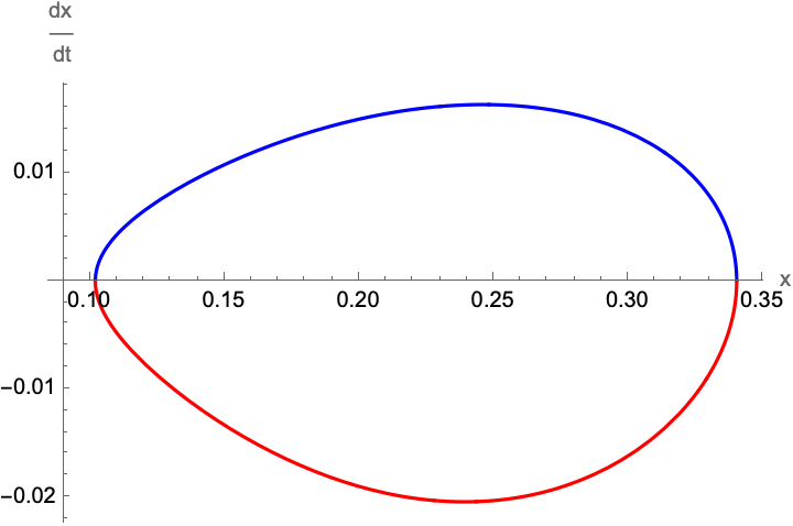
In short, the population of prey animals () grows exponentially on its own, but is limited by the presence of the predators (). The latter in turn decline exponentially on their own and only grow depending on the available prey. An exemplary numerical solution for is shown in Figure 1: the solutions never reach one of the equilibrium points at or but are in fact periodic, as can be seen from the trajectory of the system in the -plane in the right panel of Figure 1.
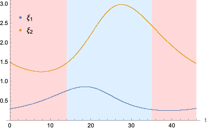
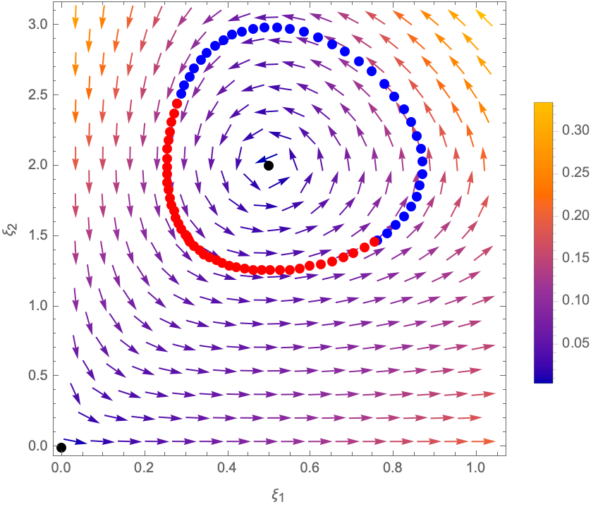
To facilitate the further discussion, we have divided the trajectory in Figure 1 into two parts (coloured red and blue respectively): to explain this, we first define the probability distribution with
| (3.2) |
The probability (which depends on time ) takes values only in a finite interval and has extrema for
| (3.3) |
On the blue portion of the trajectory, is monotonically decreasing, while on the red portion of the trajectory, is monotonically increasing, as can be seen in the left panel of Figure 2. The respective regimes in the time-evolution of the system are also indicated in red and blue respectively in the left panel of Figure 1 (and all subsequent Figures).

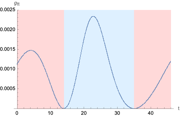
Using the probabilities (3.2), we can calculate the Fisher information metric (2.10) (which is plotted as a function of time in the right panel of Figure 2):
| (3.4) |
Following (2.19), extrema of the probability correspond to zeroes of the Fisher metric. Instead of writing the latter as a function of time , we shall now re-write it as a function of . To this end, as a first step, we can express as a function of and to obtain
| (3.5) |
However, to further express in terms of , we need to solve the dynamics of the system by integrating the quotient of the two equations in (3.1)
| (3.6) |
where is a constant that is determined by the initial conditions. Equation (3.6) can be solved to express as a function of
| (3.7) |
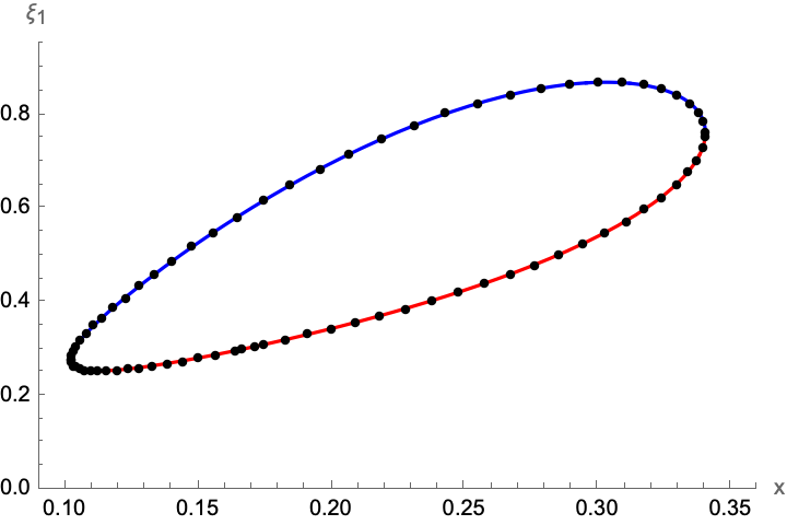
where is the Lambert function. Notice that (3.7) are in fact two solutions, corresponding to the two branches of the Lambert function, as is schematically shown in the left panel of Figure 3. These two branches are again related to the sign of (as indicated by the colouring of the plot in Figure 3). The Fisher information metric (3.5) then takes the form
| (3.8) |
which (as (3.7)) has two branches, as can be seen from the right panel of Figure 3. The zeroes of the metric are the solutions of the equation
| (3.9) |
which cannot be solved analytically for generic values of . We note, however, that the form of the metric (3.8) can be very well approximated by a function of the form
| (3.10) |
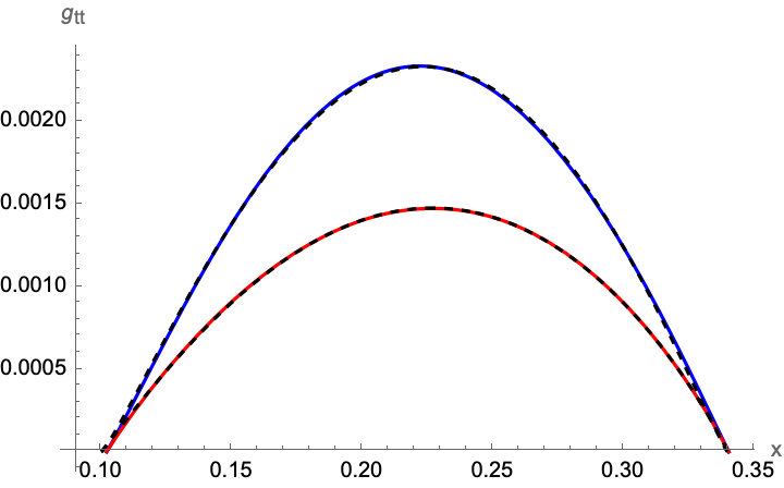
where (with ) are two real solutions of (3.9) (which are independent of time ) and suitable fitting coefficients of order 1. Indeed, an approximation of this form is shown in Figure 4, along with the flow equation
| (3.11) |
following from (2.19) (with ).
To make this approximation more tangible, we shall consider a concrete example, namely111111By defining , and , the equations (3.1) can always be brought into the form and (3.12) with . (3.13) is therefore the particular choice .
| (3.13) |
In this case, relation (3.6) allows for real solutions in terms of only for . Furthermore, (3.9) has two real solutions in the interval 121212For we have . Furthermore, the only real solutions of (3.6) arise for or , in which case, the system is in one of the two equilibrium points. In the following, we shall therefore implicitly assume .
| (3.14) |
Furthermore, the metric (3.8) takes the simpler form

| (3.15) |
which can be approximated by
| (3.16) |
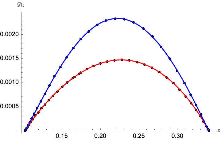
where are fit parameters that depend on : The best fits are plotted schematically in Figure 5, while explicit plots of the metric (for ) are shown in Figure 6.
3.2 SIR(S) Model
We next consider a simple compartmental model in epidemiology that describes the spread of a pathogen through a population. Here, we only consider the spread of a single pathogen, while in the following Subsections, we shall consider multiple different variants at the same time.
We assume a(n isolated) population of constant size (normalised to 1), which we group into different compartments, regarding to their state of affliction with the pathogen: we denote with the number of susceptible individuals, with the number of infectious individuals and with the number of removed individuals at time .131313Here we define as a susceptible an individual, who is currently not infectious (i.e. not inflicted by the pathogen), but may become so if in contact with an infectious individual. In contrast, a removed individual is also not currently infectious but may also not become infectious upon contact with an infectious one. We assume these numbers to be (differentiable) functions of time , whose evolution is governed by [13]
| (3.17) |
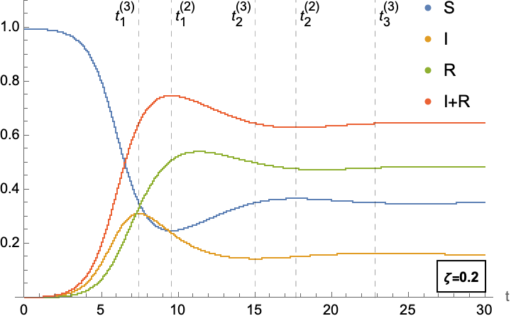
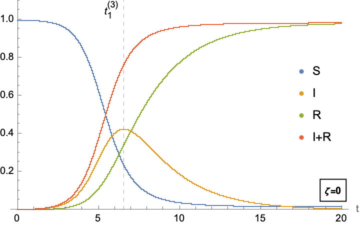
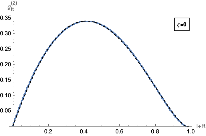
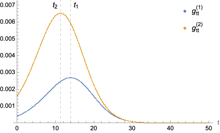
and we choose initial conditions such that . Furthermore, , , are constant parameters, which denote the rate at which susceptible individuals are infected, the rate at which infectious individuals become removed and the rate at which removed individuals become susceptible again141414The model with is usually referred to as the SIR model [13], while the model with , i.e. with the possibility of re-infection, is sometimes called the SIRS model (see e.g. [20] for a review)., respectively. A numerical solution of (3.17) (distinguishing and =0) is shown in Figure 7.
Given the initial condition (and the fact that (3.17) preserves the size of the population), such that , we can define different probability distributions that satisfy the normalisation condition (2.1). While a natural choice is to define (using the definition (2.13))
| with | (3.18) |
in order to make contact with the formalism described in Section 2.2, we shall be more interested in probability distributions as maps . Concretely, we shall consider two particular choices
| with | ||||||
| with | (3.19) |
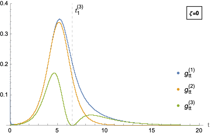
Notice, in the case , describes the cumulative number of infected individuals, which has been the object of study in the eRG approach (see e.g. [30, 31, 32, 33, 34, 35, 36, 37, 21, 38, 39, 40]). For each of the probability distributions, we also introduce the Fisher information metrics (2.10)

| (3.20) |
which are plotted as functions of time in Figure 8.151515Notice that (blue curve in Figure 8) is always large than or (orange and green curve). This follows on general grounds, since can be obtained as sums of : indeed, following [6, 41, 42] let , be discrete sets and a map, which allows to associate with each probability distribution on a probability distribution on . If we denote by the induced Fisher metric associated with , then is positive semidefinite. Since and are probability distributions defined on a set of cardinality , the flow equation (2.19) (with ) can be applied without any additional approximations (since (2.17) is automatically satisfied). Indeed, we can write
| (3.21) | |||
| (3.22) |
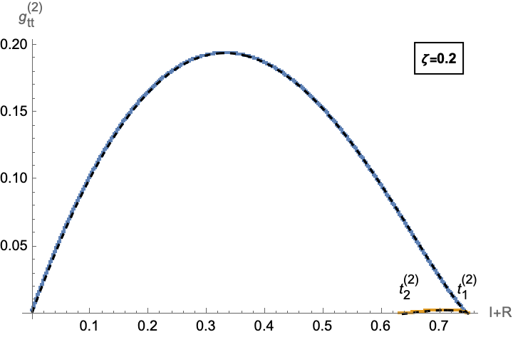
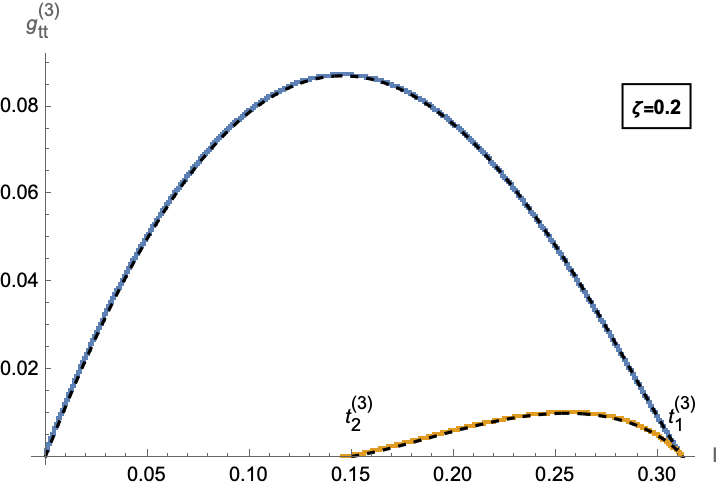
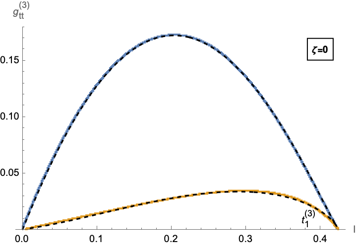
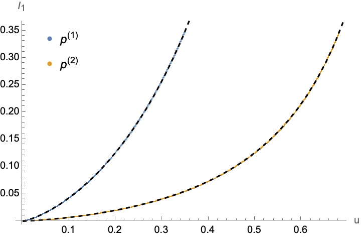
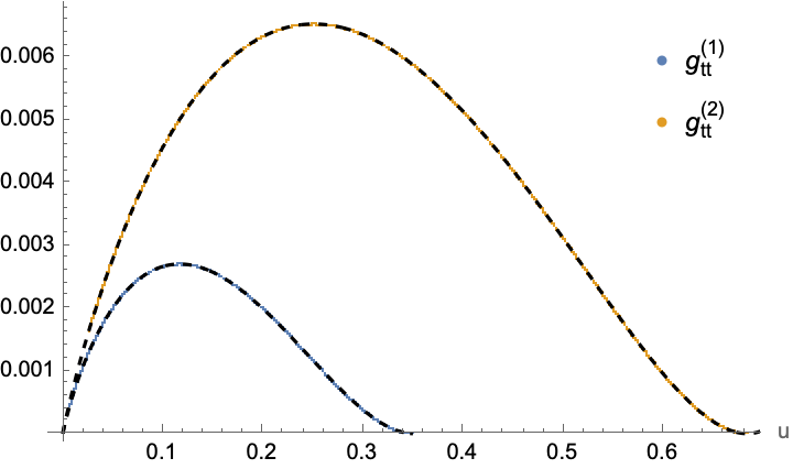
where the sign can change during the different phases of the spread of the disease. In order for these equations to fully encode (part of) the dynamics of the system, the metrics need to be expressed in terms of the probabilities themselves. This is shown for a numerical solution in Figure 9 for a model with reinfection and Figure 10 for a model without reinfection. We remark, although the model is not periodic, the schematic form of the metrics is similar to the shape found in Figure 4 in the Lotka Volterra model: indeed the dashed black lines give interpolations of all cuves with functions of the form (3.10). At least for the blue curves (which describe the initial phase of the epidemic, in which or are monotonically growing), the powers and are close to .
For both and , the exact form of the metrics in Figures 9 and 10 depends not only on the parameters , and , but also on the exact initial conditions. In the case of (i.e. a model without re-infection) we can make this concrete by solving the dynamics analytically. To this end, we consider the two probability distributions and separately:
-
•
metric : We start with the discussion of the metric in the second line of (3.20). Let , such that for
(3.23) which is not only a function of due to the presence of the factor : in fact, precisely by replacing this factor by a function of we encode the non-trivial dynamics and turn (2.19) into a non-trivial flow equation (rather than a mere definition of ). To obtain , we divide the second and third equations in (3.17)
such that (3.24) This differential equation can be integrated by taking into account the initial conditions (since we are assuming )
(3.25) Inserting this into (3.23) we therefore find the metric as a function of as well as and the initial conditions
(3.26) We have verified that the dynamics (3.25) is indeed compatible with the numerics discussed above and in particular that the form of the metric (3.26) indeed matches the numerical form plotted in the left panel of Figure 10. Notice in particular, since is monotonically growing for the entire dynamics, the metric has only a single branch. Furthermore, the metric has zeroes at
(3.27) which are in fact two values due to the two branches of the Lambert function.
-
•
metric : We can repeat the above analysis for the metric in the third line of (3.20). Let this time , such that for
(3.28) In order to express entirely in terms of , we need to resolve the dynamics by expressing as a function of . To this end, we divide the first and third equation in (3.17)
such that (3.29) This differential equation can be integrated, where we consider the initial conditions
(3.30) This relation can be inverted to express as a function of
(3.31) where is the Lambert function. Notice, however, that this solution is not unique, but has two branches, reflecting the fact that is not a monotonic function throughout the entire time evolution. Indeed, the metric takes the form
(3.32) and also has two different branches. This is indeed, what we find from the numerical solution of (3.17), which is plotted in the right panel of Figure 10.
We only briefly remark that generalising the discussion for the case (for example for the metric ) is more difficult, due to the fact that the differential equation (3.24) becomes
| (3.33) |
which is no longer directly integrable. However, a numerical solutions (see Figure 9) can nevertheless be obtained, which again reveals a metric that is piecewise of the form (3.10).
3.3 S Model
Combining (and generalising) the ideas of both the Lotka-Volterra model in Section 3.1 and the SIR model in Section 3.2, we next consider a simple compartmental model with multiple variants of the pathogen. Concretely, we denote the number of susceptible individuals at time and the number of infectious individuals who are infected with the th variant, with (for with ). We assume that each infectious carries exactly one variant and cannot be infected with any of the other variants. Here, we also exclude the possibility of recovery (we shall discuss the generalisation in the next Subsection), such that the dynamics of the epidemiological process is described by the following coupled differential equations
| and | (3.34) |
Here are constants that describe the infection rate of the th variant. We furthermore consider initial conditions at such that and therefore (since ), the size of the population remains constant. For the system (3.34) we can define various different probability distributions. Here we shall be interested in two in particular
| with | |||||
| with | (3.35) |
corresponding to the (normalised) distribution of (all) infectious individuals or individuals newly becoming infectious at time (’newly infected’) among all variants, respectively. The metrics (2.10) associated with these probability distributions can be expressed explicitly in terms of as follows
| and | (3.36) |
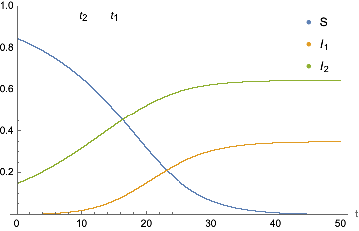
A typical time evolution of a solution of (3.34) for the simplest example (of multiple variants) is schematically shown in the left panel of Figure 11 and the metrics (3.36) are plotted in the right panel: here variant 2 was chosen to be more infectious than variant 1, but has a much lower initial condition. Such a setup models the emergence of a new variant (the more infectious variant 2) in a population where variant 1 is already established. One can generalise such a scenario to simulate the emergence of a new variant in a population where already several others are circulating. To this end we shall label the number of infectious in (3.34) in a slightly different fashion: let with and let
| (3.37) |
which simulates the emergence of a more infectious variant (called variant 1) in the presence of an already established class of very similar variants. In this case, the summations in (3.36) can be approximated by
| and | (3.38) |
where we have defined
| and | (3.39) |
which are respectively the average infection rate of the variants and their combined number of infectious individuals. The metrics (3.38), however, are exactly the Fisher metrics for two variants . Thus, from the perspective of the information in the system, the variants combined behave essentially as a single one (which justifies the use of clustering tools as used for example in [40]).
We next model the dynamics of the emergence of a new variant using the flow equation (2.19) by expressing the metrics in(3.39) as a function of the probability distributions. As explained above, we shall consider the case in (3.34) as approximation for a new variant (variant 1) emerging among already established ones, which collectively behave as variant 2. We can treat both probability distributions in (3.35) in parallel by defining
| (3.42) |
and therefore the metric becomes
| (3.43) |
To write these metrics entirely as functions of or , we need to resolve the dynamics of the system to express as a function of or respectively. To this end, we divide the two equations (3.34)
| (3.46) |
such that
| with | (3.49) |
We can integrate this equation with the initial conditions
| and | (3.52) |
to find
| (3.53) |
which leads to
| (3.54) |
The form of this solution is compared with the numerical solutions discussed above in the left panel of Figure 12. Furthermore, the metrics become
| (3.55) |
which are compared to the numerical results in the right panel of Figure 12. We note that the metrics (3.55) can be well approximated by a function of the form (3.10) with
| (3.58) |
3.4 SR(S) Model
As a generalisation of the S model discussed in the previous Subsection, we now consider an SR(S) model, in which infectious individuals may recover (and potentially may become re-infected at a later time). To this end, in addition to and (with ) we introduce as further compartment the number of removed (recovered) individuals at time . As before, we consider variants, with (slightly) different properties regarding infection and removal:
| (3.59) |
with denoting the infection and recovery rates of the th variant and the rate at which removed individuals become susceptible again. We furthermore assume initial conditions at time such that . For the model (3.59) we shall consider the following various probability distributions
| with | |||||
| with | |||||
| with | (3.60) |
corresponding to the normalised distribution of infectious individuals, individuals becoming infectious (’newly infected’) and individuals recovering, respectively. The associated Fisher information metrics (2.10) take the form
| (3.61) |
These metrics can be written in a unified form as a function of the probabilities
| (3.62) |
where we have used for the probabilities (3.60). The combinations
| (3.63) |
depend on , such that (3.62) is not a function of the (and thus the ) alone. Following (2.15), the metric can also be represented in the following factorised form
| (3.64) |
Comparing (3.64) with (3.62) indeed allows to express the dynamics of the as161616Since (3.64) is bilinear in the derivatives of , there remains a sign ambiguity which is related to the direction of time.
| (3.67) |
which still implicitly depends on . Notice also that the probabilities are not necessarily monotonic functions. For , this can be seen by writing the time-derivatives in the following manner171717Here we implicitly assume .
| (3.68) |
Since is not positive definite, but , the sign of the time-derivatives of the probabilities are not fixed.
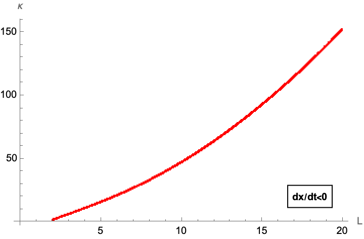
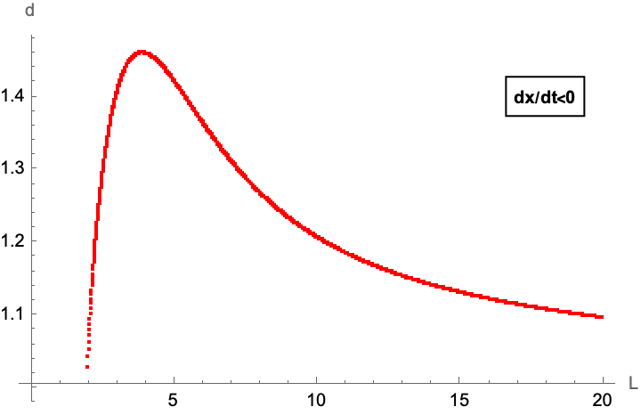
As in the previously discussed examples, in order to write (3.67) as an effective model for the dynamics of the system, we need to resolve the dynamics. In the present case, we shall do so in the particular case and provide numerical solutions of the metric as functions of in Figure 13. The dashed black lines give approximations of the metrics following (3.10). Specifically, for (left panel) we find as best fits
| (3.69) |
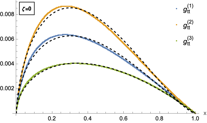
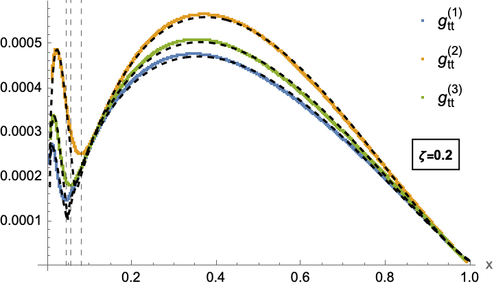
while for (right panel) we find the approximation
| (3.72) | ||||
| (3.75) | ||||
| (3.78) |
We remark that another way to fit these metrics is of the form
| (3.79) |
with real- and a complex zero (and suitable fitting parameters). Concretely, for the right panel of Figure 13 we find
| (3.80) |
Finally, before closing this Section we remark that for ,181818Similarly we may assume as in (3.37) that several variants behave very similarly and can thus be modelled collectively. we can find exact expressions of as functions of respectively in particular cases: for example we may impose that and remain (approximately) constant
| and | (3.81) |
In this case the overall number of infectious individuals remains constant and only the distribution between the two variants changes. The conditions (3.81) are solved by
| and | (3.82) |
which allows us to simplify the expressions for the metrics:
| with | ||||||
| with | ||||||
| with | (3.83) |
In all three cases, the solution of (2.19) (with ) yields the following transcendental equations for as a function of time
| (3.84) |
4 General Metric
In the previous Section, we have re-organised the dynamics of a number of simple examples in the form of the flow equation (2.19). To this end, we have defined probability distributions for this models of the form with and have expressed the metric as a function of . In all cases, we have seen that the latter can (at least piecewise) be very well approximated by a function of the form (3.10) with constants of order . In this Section we consider the inverse problem, i.e. we start with the simplest form of the metric (3.10) and develop the corresponding dynamics in an analytic fashion.
4.1 Monotonic Evolution
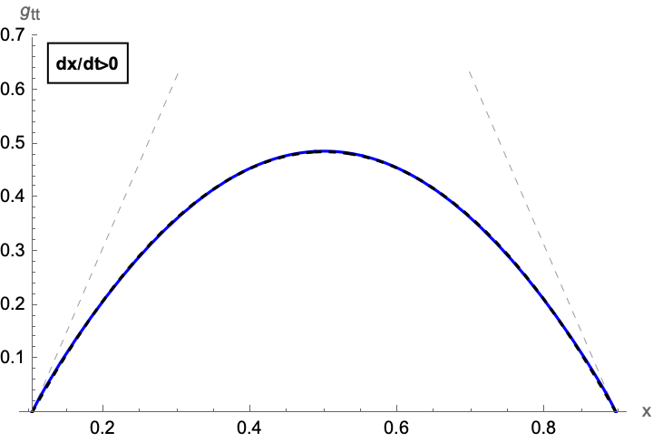
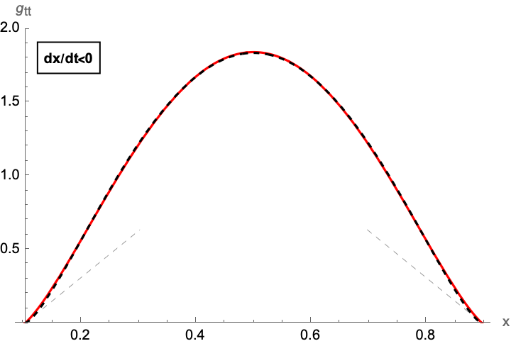
We start by considering the following simple form of the metric
| for | (4.3) |
i.e. (3.10) for the simplest case . We assume this metric as the defining input for the dynamics, which fixes according to the flow equation (2.19) for . Assuming the initial condition 191919The case or needs particular care, as we shall discuss below., the flow equation can be integrated
| (4.4) |
where we have assumed that the sign of the first derivative of remains constant for all times in the interval and . Furthermore, in (4.4) is the incomplete elliptic integral of the first kind
| (4.5) |
with the arguments
| and | (4.6) |
The relation (4.4) can be solved to express as a function of time
| (4.7) |
where sn is a Jacobi elliptic function, which can be expressed in terms of Jacobi theta-functions
| with | (4.8) |
The solution (4.7) is periodic in with periodicity
| (4.9) |
where is the complete elliptic integral of the first kind
| (4.10) |
In the case of and care needs to be taken that only is allowed (i.e. notably ). In this case, the integral in (4.4) simplifies
| (4.11) |
such that
| (4.12) |
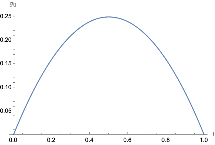
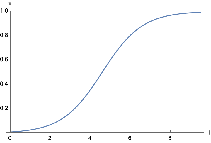
which corresponds to a logistic function and is plotted schematically in Figure 14. Notice that
| (4.15) |
such that the function is monotonic for the entire time evolution.
4.2 Full Time Evolution
Using the result of the previous Subsection, we can construct more complicated time evolutions, by defining the metric to be piecewise of the form (4.3).
4.2.1 Flow Between Real Zeroes of the Metric
Notice that the integral (4.4) is only defined for (since outside of this interval the integrand becomes imaginary) and for fixed sign of the time derivative . In the examples of Section 3, we have seen that the zeroes of the metric or , correspond to points, where the sign of changes, which also leads to a change in the metric. Thus, in this case, we can describe the time evolution by defining the metric piecewise, for fixed sign of . In the following we discuss two examples in more detail: the first one inspired by the Lotka-Volterra equation in Section (3.1) and the second one inspired by the SIR model in Section 3.2:
-
1.
Periodic Time Evolution: We first shall consider a metric of the form
(4.20) where both zeroes of the two branches of the metric coincide (see left panel of Figure 15).
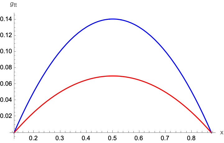
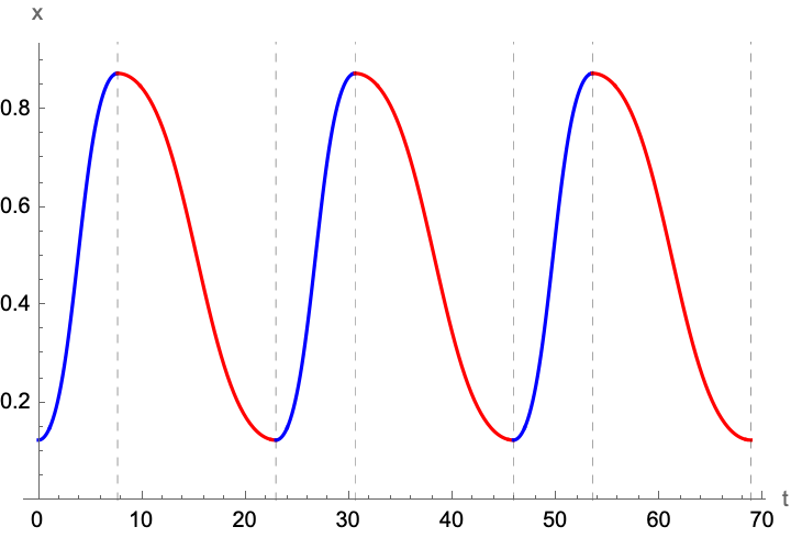
Figure 15: Left panel: Metric (4.20) for , , (blue curve) and (red curve). Right panel: corresponding dynamics (4.12) for and . The dashed lines indicate extrema of , corresponding to zeroes of the metric (i.e. points where the branch of the metric changes). The colours of the dynamics in the right panel match the colours of the branch of the metric in the left panel. -
2.
Oscillating Time Evolution: Let and be two (convergent) series of real integers, such that and . Then consider the series of metrics
(4.26) This series of metrics then describes a time evolution, where oscillates around and is piecewise described by (4.7). An example for the series
(4.27) (and ) is shown in Figure 16, leading to a solution oscillating around .
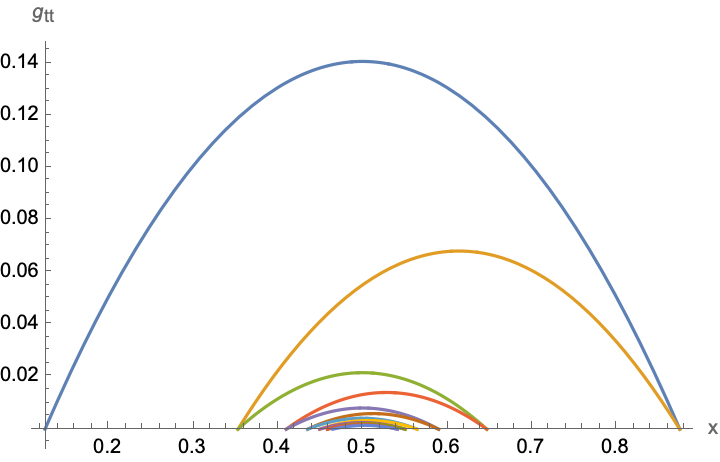
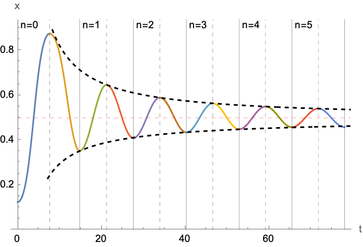
Figure 16: Metric (4.26) (left) and evolution of (right) using the series (4.27) and initial conditions and . The black vertical lines indicate extrema of , corresponding to zeroes of the metric: solid lines mark the increase , while the dashed lines mark the switch of the branch of the metric in (4.26). The colours of the dynamics in the right panel match the colours of the branch of the metric in the left panel.
4.2.2 Flow Between Imaginary Zeroes of the Metric
Before closing this Section, we want to remark on another possibility for defining metrics that are piecewise of the form (4.3): in the previous examples, we have glued metrics at their (real) zeros, corresponding to extrema of . In principle, we can also glue metrics along points with , an example of which we have encountered in Section 3.4 (see right panel of Figure 13) in the time evolution of the SR model with re-infection. A simpler example is given by the dashed black curve in the left panel of Figure 17 (black dashed curve). This metric is approximated by a function of the form
| with | (4.30) |
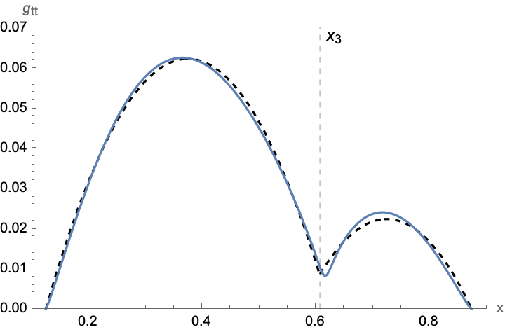
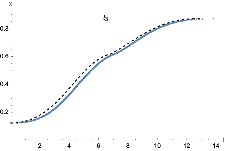
where are suitable fitting parameters and real zeroes of , while (and its conjugate ) are complex zeroes. From this perspective, the metric is joined along a complex zero and is not convex on the entire interval . The solution of (2.19) for the piecewise defined is shown in the right panel of Figure 17 (black dashed curve), along with a numerical solution using the approximated metric (4.30). Indeed, the sign of remains positive for the entire time evolution, consistent with the fact that the metric never vanishes. Such a behaviour was used in [34] to model periods between two waves of a SARS-CoV-2 epidemic. This behaviour was re-interpreted in [21] as a system coming close to a(n unstable) fixed point in the context of multiple variants of SARS-CoV-2.
5 Conclusions
In this paper we have studied a reformulation of simple epidemiological- and population dynamical processes in terms of the Fisher information (metric). To this end, we have first re-organised the degrees of freedom of the system into (normalised) probability distributions (in the sense of (2.1)) that are functions of time. This is a natural step in epidemiology or population dynamics, since in many approaches a given population is grouped into distinct classes (see e.g. compartmental models [13]) and probabilities can be defined as normalised ratios of their sizes. We have associated the Fisher information [1] with a chosen probability distribution, which (following [2, 3, 4, 5, 6]) we have interpreted as a metric of a one-dimensional Riemannian manifold, to highlight its property to capture the distance between the state of the system at different times. In fact, for configurations where the entire probability distribution can be described by a single bounded function (with ), we have shown that the dynamics can be re-cast in the flow equation (2.19), which is entirely determined by the metric. Partially resolving the dynamics of various different models, namely the Lotka-Volterra model (Section 3.1), the SIR(S) model (Section 3.2) and compartmental models describing the evolution of two (or more) variants of a disease (Sections 3.3 and 3.4), such that can be expressed as a function of alone, has revealed strong similarities between the different models: the time evolution of can be described piecewise for regimes in which is a monotonic function, i.e. between two of its local extrema, which correspond to real zeroes of . Moreover, in any such regime the metric can be very well approximated simply through powers of its zeroes: if is a convex function it can be approximated through the form (3.10), which can be generalised by including imaginary zeroes (see (4.30)) if has one or more local minima. The complete dynamics of the system can be described by gluing such metrics together at their zeroes. In fact, using such a metric as a full input for the flow equation (2.19) and focusing on the simplest type of metric (i.e. (4.3)) we have provided an analytic, closed form solution of the monotonic time evolution for in (4.7). By gluing this solution, we have constructed more general periodic and oscillating solutions in Section 4.2.
Our approach highlights that the Fisher information metric not only describes families of probabilities, but in fact is capable of capturing their full time evolution provided that enough information about the dynamics of the system can be encoded in it. In our current setting, where the probability distribution is described as a single function , this is tantamount to re-writing as a function of alone, rather than an explicit function of . The emerging dynamics is quite similar among very different looking models, since details of the system have been resolved, thus revealing universal properties of the underlying time evolution. Specifically, our analysis reveals the importance of zeroes of the metric, both real and imaginary: real zeroes correspond to extrema of the probability distribution and specifying the metric between two zeroes fixes a monotonic time evolution of . Complex zeroes (or local minima) of provide additional structure (resembling saddle points) to this monotonic time evolution, as can be seen in the right panel of Figure 17.
The importance of (quasi) fixed points in the time evolution was previously pointed out in [34, 21] in a concrete epidemiological system: inspired by ideas of renormalisation group methods [43, 44, 45, 46, 47, 48] the (M)eRG (Mutation epidemiological Renormalisation Group) model (based on an original proposal in [30, 31]) conjectured a (set of) first order differential equations (called -functions or flow equations) that interpolate the cumulative number of individuals infected with (a variant of) a disease between two (disease free) fixed points. This simple model was very successful in describing individual waves of Covid-19 in various regions of the world [32, 33, 36, 37, 39] (see also the review [38]), while the multi-wave structure was attributed to unstable fixed points of the system [35, 34] which were linked to the appearance of new variants of SARS-CoV-2 replacing previous ones [21]. Our current analysis is not only in line with this interpretation, but in fact gives a clearer picture of how to describe the notion of ’fixed point’ in a more general class of systems: by reducing the dynamics of quite different models (with conceptually different degrees of freedom) to a common form (2.19), we can translate the notion of a ’fixed point’ (in the language of [34, 21]) to (complex) zeroes of the Fisher information, for which moreover a geometric interpretation exists. This allows to re-organise the dynamics of a much larger class of quite different models around these ’fixed points’, as is evidenced by our simple approximations in (3.10). Moreover, this re-formulation leads to a potentially simpler description (focused on properties of the system around highly symmetric points), as is showcased by the analytic solutions we have found for the simplest approximation in Section 4.
For the future, we anticipate further applications and generalisations of our work. First of all it will be interesting to extend the description to include cases where the (effective) probability distribution is described by more than one function . Similarly, the inclusion of additional parameters beyond the time-variable will lead to more refined Fisher metrics, capable of describing more sophisticated models and their fixed points.
Acknowledgements
This study is supported by Ministero dell’Università e della Ricerca (Italy), Piano Nazionale di Ripresa e Resilienza, and EU within the Extended Partnership initiative on Emerging Infectious Diseases project number PE00000007 (One Health Basic and Translational Actions Addressing Unmet Needs on Emerging Infectious Diseases). The work of F.S. is partially supported by the Carlsberg Foundation, semper ardens grant CF22-0922.
References
- [1] R. A. Fisher and E. J. Russell, “On the mathematical foundations of theoretical statistics,” Philosophical Transactions of the Royal Society of London. Series A, Containing Papers of a Mathematical or Physical Character, vol. 222, no. 594-604, pp. 309–368, 1922.
- [2] H. Hotelling, “Spaces of statistical parameters,” Bulletin of the American Mathematical Society (AMS), vol. 36, p. 191, 1930.
- [3] R. C. Rao, “Information and the accuracy attainable in the estimation of statistical parameters,” Bulletin of the Calcutta Mathematical Society, vol. 37, pp. 81–91, 1945.
- [4] H. Jeffreys, “An invariant form for the prior probability in estimation problems,” Proc. R. Soc. Lond. A, vol. 186(1007), pp. 453–461, 1946.
- [5] S. L. Lauritzen, “Statistical manifolds,” Differential geometry in statistical inference, vol. 10, pp. 163–216, 1987.
- [6] S. Amari and H. Nagaoka, Methods of Information Geometry. Translations of mathematical monographs, American Mathematical Society, 2000.
- [7] S.-I. Amari, “A foundation of information geometry,” Electronics and Communications in Japan (Part I: Communications), vol. 66, no. 6, pp. 1–10, 1983.
- [8] S. Amari, “Information geometry,” Contemporary Mathematics, vol. 203, pp. 81–96, 1997.
- [9] S. Amari, Differential-Geometrical Methods in Statistics. Lecture Notes in Statistics, Springer New York, 2012.
- [10] S.-i. Amari, Information Geometry and Its Applications. Springer Publishing Company, Incorporated, 1st ed., 2016.
- [11] A. J. Lotka, “Contribution to the theory of periodic reactions,” The Journal of Physical Chemistry, vol. 14, pp. 271–274, 1909.
- [12] V. Volterra, “Variazioni e fluttuazioni del numero d’individui in specie animali conviventi.,” Mem. Acad. Lincei Roma., vol. 2, pp. 31–113, 1926.
- [13] W. O. Kermack, A. McKendrick, and G. T. Walker, “A contribution to the mathematical theory of epidemics,” Proceedings of the Royal Society A, vol. 115, pp. 700–721, 1927.
- [14] N. Bailey, The Mathematical Theory of Infectious Diseases, 2nd ed. Hafner, New York, 1975.
- [15] N. Becker, “The use of epidemic models,” Biometrics, vol. 35, pp. 295–305, 1978.
- [16] K. Dietz and D. Schenzle, “Mathematical models for infectious disease statistics, in: A. Atkinson (Ed.), A Celebration of Statistics,” Springer, pp. 167–204, 1985.
- [17] C. Castillo-Chavez, “Mathematical and Statistical Approaches to AIDS Epidemiology, Lecture Notes in Biomath,” Springer-Verlag, Berlin, vol. 83, 1989.
- [18] K. Dietz, “Epidemics and rumours: A survey,” J. Roy. Statist. Soc. Ser. A, vol. 130, pp. 505–528, 1967.
- [19] K. Dietz, “Density dependence in parasite transmission dynamics,” Parasit. Today, vol. 4, pp. 91–97, 1988.
- [20] H. Hethcote, “A thousand and one epidemic models, in Frontiers in Theoretical Biology, S.A. Levin, ed., Lecture Notes in Biomath.,” Springer-Verlag, Berlin, vol. 100, pp. 504–515, 1994.
- [21] G. Cacciapaglia, C. Cot, A. de Hoffer, S. Hohenegger, F. Sannino, and S. Vatani, “Epidemiological theory of virus variants,” Physica A, vol. 596, p. 127071, 2022.
- [22] A. Lesne, “Shannon entropy: a rigorous notion at the crossroads between probability, information theory, dynamical systems and statistical physics,” Mathematical Structures in Computer Science, vol. 24, no. 3, p. e240311, 2014.
- [23] T. M. Cover and J. A. Thomas, Elements of Information Theory (Wiley Series in Telecommunications and Signal Processing). USA: Wiley-Interscience, 2006.
- [24] I. Csiszár, “Information-type measures of differences of probability distributions and indirect observations,” Studia Sci. Math. Hungarica, vol. 2, pp. 299 – 318, 1967.
- [25] I. Csiszár, “On topological properties of -divergence,” Studia Sci. Math. Hungarica, vol. 2, pp. 329 – 339, 1967.
- [26] F. Nielsen, “An elementary introduction to information geometry,” Entropy, vol. 22, no. 10, 2020.
- [27] S. Kullback and R. A. Leibler, “On Information and Sufficiency,” The Annals of Mathematical Statistics, vol. 22, no. 1, pp. 79 – 86, 1951.
- [28] J. Burbea and C. Rao, “Entropy differential metric, distance and divergence measures in probability spaces: A unified approach,” Journal of Multivariate Analysis, vol. 12, no. 4, pp. 575–596, 1982.
- [29] H. K. Miyamoto, F. C. C. Meneghetti, and S. I. R. Costa, “On closed-form expressions for the fisher-rao distance,” 2023.
- [30] M. Della Morte, D. Orlando, and F. Sannino, “Renormalization Group Approach to Pandemics: The COVID-19 Case,” Front. in Phys., vol. 8, p. 144, 2020.
- [31] M. Della Morte and F. Sannino, “Renormalisation Group approach to pandemics as a time-dependent SIR model,” Front. in Phys., vol. 8, p. 583, 2021.
- [32] G. Cacciapaglia, C. Cot, and F. Sannino, “Second wave covid-19 pandemics in europe: A temporal playbook,” Sci Rep, vol. 10, p. 15514, 2020.
- [33] G. Cacciapaglia, C. Cot, and F. Sannino, “Mining google and apple mobility data: Temporal anatomy for covid-19 social distancing,” Scientific Reports, vol. 11, p. 4150, 2021.
- [34] G. Cacciapaglia and F. Sannino, “Evidence for complex fixed points in pandemic data,” Front. Appl. Math. Stat., vol. 7, p. 659580, 2021.
- [35] G. Cacciapaglia, C. Cot, and F. Sannino, “Multiwave pandemic dynamics explained: How to tame the next wave of infectious diseases,” Scientific Reports, vol. 11, p. 6638, 2021.
- [36] G. Cacciapaglia and F. Sannino, “Interplay of social distancing and border restrictions for pandemics (COVID-19) via the epidemic Renormalisation Group framework,” Sci Rep, vol. 10, p. 15828, 5 2020.
- [37] G. Cacciapaglia, C. Cot, A. S. Islind, M. Óskarsdóttir, and F. Sannino, “Impact of us vaccination strategy on covid-19 wave dynamics,” Scientific Reports, vol. 11(1), pp. 1–11, 2021.
- [38] G. Cacciapaglia, C. Cot, M. Della Morte, S. Hohenegger, F. Sannino, and S. Vatani, “The field theoretical ABC of epidemic dynamics,” 1 2021.
- [39] S. Hohenegger, G. Cacciapaglia, and F. Sannino, “Effective mathematical modelling of health passes during a pandemic,” Scientific Reports, vol. 12, p. 6989, 2022.
- [40] A. de Hoffer, S. Vatani, C. Cot, G. Cacciapaglia, M. L. Chiusano, A. Cimarelli, F. Conventi, A. Giannini, S. Hohenegger, and F. Sannino, “Variant-driven multi-wave pattern of covid-19 via a machine learning analysis of spike protein mutations,” Sci Rep, vol. 12, p. 9275, 2022.
- [41] S. Amari, O. E. Barndorff-Nielsen, R. E. Kass, S. L. Lauritzen, and C. R. Rao, “Differential Geometry in Statistical Inference,” Lecture Notes-Monograph Series, vol. 10, pp. i – 240.
- [42] S.-I. Amari, “Differential Geometry of Curved Exponential Families-Curvatures and Information Loss,” The Annals of Statistics, vol. 10, no. 2, pp. 357 – 385, 1982.
- [43] G. Barenblatt, “Self-similarity: Similarity and intermediate asymptotic form,” Radiophysics and Quantum Electronics, vol. 19, pp. 643–664, 1976.
- [44] G. I. Barenblatt, Scaling, Self-similarity, and Intermediate Asymptotics: Dimensional Analysis and Intermediate Asymptotics. Cambridge Texts in Applied Mathematics, Cambridge University Press, 1996.
- [45] N. Goldenfeld, O. Martin, and Y. Oono, “Intermediate asymptotics and renormalization group theory,” J. Sci. Comput., vol. 4, pp. 355–372, 12 1989.
- [46] N. Goldenfeld, Lectures On Phase Transitions And The Renormalization Group. CRC Press, 2018.
- [47] L.-Y. Chen, N. Goldenfeld, and Y. Oono, “Renormalization group and singular perturbations: Multiple scales, boundary layers, and reductive perturbation theory,” Physical Review E, vol. 54, p. 376–394, Jul 1996.
- [48] Y. Oono, In Advances in Chemical Physics; Prigogine, I., Rice, S. A., Eds. Wiley: New York, 1985.