Uncertainty Quantification in Anomaly Detection
with Cross-Conformal $p$-Values

Abstract

Given the growing significance of reliable, trustworthy, and explainable machine learning, the requirement of uncertainty quantification for anomaly detection systems has become increasingly important. In this context, effectively controlling Type I error rates ($\alpha$) without compromising the statistical power ($1-\beta$) of these systems can build trust and reduce costs related to false discoveries, particularly when follow-up procedures are expensive. Leveraging the principles of conformal prediction emerges as a promising approach for providing respective statistical guarantees by calibrating a model’s uncertainty.
This work introduces a novel framework for anomaly detection, termed cross-conformal anomaly detection, building upon well-known cross-conformal methods designed for prediction tasks. With that, it addresses a natural research gap by extending previous works in the context of inductive conformal anomaly detection, relying on the split-conformal approach for model calibration. Drawing on insights from conformal prediction, we demonstrate that the derived methods for calculating cross-conformal $p$-values strike a practical compromise between statistical efficiency (full-conformal) and computational efficiency (split-conformal) for uncertainty-quantified anomaly detection on benchmark datasets.

1 Introduction

The field of anomaly detection, also referred to as novelty detection, has been steadily gaining interest in both the scientific community (Pimentel et al., 2014; Pang et al., 2021) and wider industry, with critical applications in fraud detection (Hilal et al., 2022), cybersecurity (Evangelou & Adams, 2020), predictive maintenance (Carrasco et al., 2021) and health care (Fernando et al., 2021), among others. Despite the general interest and importance for many industry applications, the necessity of uncertainty quantification in this context has only recently been recognized, with the emergence of reliable (Smuha, 2019), trustworthy (Chen et al., 2022), and explainable machine learning (Belle & Papantonis, 2021).

In this work, we primarily focus on the unsupervised approach of one-class-classification (Petsche & Gluck, 1994; Japkowicz et al., 1999; Tax, 2001) for anomaly detection — in the sense that only non-anomalous observations are used to train an anomaly detection model. This approach is particularly suitable when a representative set of anomalous observations is not available, as to be expected in most anomaly detection settings.

One problem most algorithms commonly used for one-class-classification share, is that they do not come with statistical guarantees regarding their anomaly estimates. With that, an estimator’s uncertainty and resulting error probabilities can not be quantified, undermining its trustworthiness.
Conformal anomaly detection can address this problem by leveraging the non-parametric and model-agnostic framework provided by conformal prediction (Papadopoulos et al., 2002; Vovk et al., 2005; Lei & Wasserman, 2013), which has recently gained renewed attention as a reliable approach to uncertainty quantification. As shown in preceding works, corresponding conformalized methods for prediction tasks can in principle be adapted for the application in anomaly detection without compromising the statistical validity of the underlying concept (Laxhammar & Falkman, 2010; Laxhammar, 2014).

Conformal prediction was originally proposed to allow for distribution-free uncertainty quantification for regression tasks (using prediction intervals) and classification tasks (using prediction sets) that guarantees a $1-\alpha$ coverage of the true value or class given a significance level $\alpha$. Guarantees by conformal methods hold when training and test data are said to be exchangeable. Exchangeability is a statistical term, closely related but weaker than the assumption of independent and identically distributed variables ($i.i.d.$).
In one of the most basic approaches of conformal prediction, the so-called (non-)conformity scores (e.g. residual values, class probability scores, …) obtained by a scoring function (an estimator) are calibrated on a hold-out set, separated from the training data, providing a means to assess the model’s confidence in its predictions objectively. This approach is said to be split-conformal, otherwise known as inductive conformal prediction.

In this work we focus on cross-conformal methods, which represent a “hybrid of the methods of inductive conformal prediction and cross-validation” (Vovk, 2013a). With that, cross-conformal methods address notorious problems like overfitting and estimator instability (Andrews, 1986) due to data variability. Respective methods also make more efficient use of available training data, since the dedicated holdout set of the inductive approach becomes dispensable. Cross-conformal methods may particularly be interesting when working with smaller training datasets ($n\ll 10.000$).

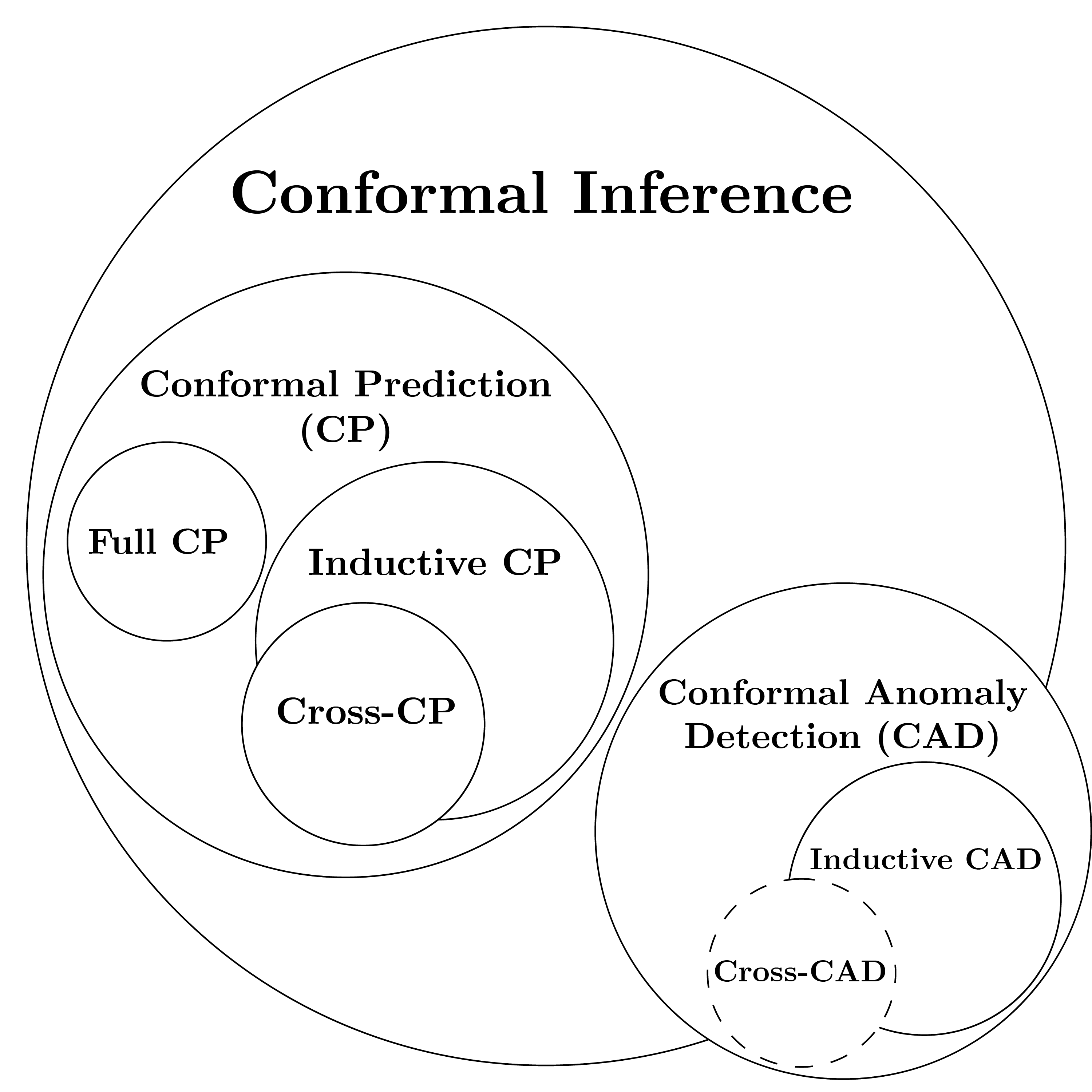
Figure 1: Non-exhaustive taxonomy of conformal inference with conformal prediction and the derived conformal anomaly detection including the current research gap of cross-conformal anomaly detection based on cross-conformal prediction.

The majority of (cross-)conformal prediction methods can be adapted for the application within the field of anomaly detection while maintaining statistical validity, as we demonstrate in this work. The lack of respective mathematical formulations and practical demonstrations, particularly for cross-conformal anomaly detectors, represents a natural research gap (see Figure 1).

The general necessity of conformalized methods for anomaly detection and other areas arises from the lack of non-parametric models, often subject to a priori assumptions, and the abundance of parameter-laden algorithms — both prone to either misspecification or overfitting (Keogh et al., 2007). Beyond that, critical (hyper-)parameters like anomaly thresholds and resulting false discovery rates (FDR) often decide whether the anomaly detection system at hand is deemed practical or not.

Contributions. Within the given context, the main contributions of this work may be summarized as follows:

• Proposal of a novel cross-conformal framework for anomaly detection, based on cross-conformal prediction, offering reliable (marginal) FDR-control while yielding more powerful anomaly detectors than the inductive conformal approach of related works.

• Derivation of five cross-conformal anomaly detection methods in analogy to their existing counterparts for conformal prediction, namely $\text{Jackknife}_{\text{AD}}$ and $\text{Jackknife+}_{\text{AD}}$, $\text{CV}_{\text{AD}}$ and $\text{CV+}_{\text{AD}}$ and the $\text{Jackknife+-after-Bootstrap}_{\text{AD}}$.

• Empirical evaluation testifying overall superior statistical power (sensitivity) of cross-conformal detectors, without breaking the (marginal) FDR-control at given nominal levels by the Benjamini-Hochberg procedure.

2 Related Work

Beyond the seminal works regarding conformal inference (Gammerman et al., 1998; Papadopoulos et al., 2002; Vovk et al., 2005; Lei & Wasserman, 2013) the term conformal anomaly detection was first introduced in (Laxhammar & Falkman, 2010) and later revisited and extended in (Bates et al., 2023), among others.

In (Laxhammar & Falkman, 2010; Laxhammar, 2014) conformal anomaly detection was initially applied for detecting anomalous trajectories in maritime surveillance applications. Both works formalized and discussed the principles of conformal prediction applied to an anomaly detection task. As part of (Laxhammar, 2014), conformal anomaly detection and inductive conformal anomaly detection were proposed without further assessing strategies beyond the inductive procedure.
Other works relying on the application of conformal anomaly detection or related (conformal) concepts are (Smith et al., 2015; Guan & Tibshirani, 2022; Haroush et al., 2022) complemented by (Fedorova et al., 2012; Ishimtsev et al., 2017; Cai & Koutsoukos, 2020; Vovk, 2020, 2021; Vovk et al., 2021), specifically dedicated to online settings. None of these works explicitly referred to or assessed variants of cross-conformal anomaly detection.

Cross-conformal methods, to be adapted for the application in anomaly detection, are namely Jackknife (Steinberger & Leeb, 2016, 2023), Jackknife+, CV, CV+ (Vovk, 2013a; Barber et al., 2021) and Jackknife+-after-Bootstrap (Kim et al., 2020). All of these methods were derived in the context of cross-conformal prediction.

The overarching framework, and the derived methods, are model-agnostic, so it is generally possible to conformalize any given anomaly detector that outputs suitable anomaly scores (see Section 3). Most well-known methods for anomaly detection (Aggarwal, 2013; Agrawal & Agrawal, 2015) adhere to this requirement.

3 Background

First, we briefly examine the widely applied and already well-described split-conformal approach for computing conformal $p$-values in the context of anomaly detection — synonymous with inductive conformal anomaly detection (Laxhammar & Falkman, 2010; Laxhammar, 2014). Establishing the fundamentals will serve as a starting point for deriving the cross-conformal methods in Section 4.

We consider an anomaly detection task given a set of observations $\mathcal{D}=\{x_{1},x_{2},...,x_{n}\}=\{X_{i}\}_{i=1}^{n}$ used for training, comprising $n$ observations $X_{i}\in\mathbb{R}^{d}$ in a $d$-dimensional feature space, sampled from an unknown continuous, discrete, or mixed distribution $P_{X}$ considered to be non-anomalous. We aim to test an unseen (non-empty) set of observations $\mathcal{D}_{\text{test}}=\{x_{n+1},x_{n+2},...,x_{n_{\text{test}}}\}=\{X_{n+i}\}_{i=1}^{n_{\text{test}}}$ assumed to be sampled from $P_{X}$ for potential anomalies.
In this context, anomalies may be characterized as either unusual (see novelty detection) or out-of-distribution, arising from a distinct underlying data-generating process.

Inductive Conformal Anomaly Detection. Initially, an anomaly scoring function $\hat{s}:\mathbb{R}^{d}\rightarrow\mathbb{R}$ is fitted on $\mathcal{D}_{\text{train}}\subset\mathcal{D}$ and subsequently calibrated on $\mathcal{D}_{\text{cal}}\subset\mathcal{D}$ which is disjoint from $\mathcal{D}_{\text{train}}$ with $\mathcal{D}_{\text{cal}}\cap\mathcal{D}_{\text{train}}=\emptyset$. Depending on the number of observations $m$ assigned to the training set $\mathcal{D}_{\text{train}}$ with $m<n$, the scoring function $\hat{s}$ is fitted on $\mathcal{D}_{\text{train}}=\{x_{1},x_{2},...,x_{m}\}=\{X_{i}\}_{i=1}^{m}$ by a suitable anomaly detection algorithm $\mathcal{A}$ as $\hat{s}=\mathcal{A}(X_{i})$ for all $X_{i}\in\mathcal{D}_{\text{train}}$.
Subsequently, $\hat{s}$ is calibrated on the remaining observations in the hold-out set $\mathcal{D}_{\text{cal}}=\{x_{m+1},x_{m+2},...,x_{n}\}=\{X_{m+i}\}_{i=1}^{n}$ by computing the calibration set as ${\hat{s}(X_{i})}$ for all $X_{i}\in\mathcal{D}_{\text{cal}}$. In practice, a calibration set of size $n-m\geq 1000$ is deemed to be sufficient for most applications (Angelopoulos & Bates, 2021).
For inference, the calibrated scoring function then assigns a score $\hat{s}(x)$, as a scalar estimate for anomalousness, to an unseen $x\in\mathcal{D}_{\text{test}}$. In this work, smaller scores $\hat{s}(x)$ indicate that $x$ might be an anomaly. The obtained score $\hat{s}(x)$ is then compared to the calibration set.
With that, the (split-)conformal $p$-values of any new observation $x$ is computed by

$$p(x)=\frac{\lvert\{i\in\mathcal{D}_{\text{cal}}\ :\ \hat{s}(X_{i})\leq\hat{s}(x)\}\rvert+1}{\lvert\mathcal{D}_{\text{cal}}\rvert+1}$$ (1)

with applied additively smoothing adjustment function

$$p(x)=\frac{nx+1}{n+1}$$ (2)

to ensure the superuniform nature of computed $p$-values, as discussed in the following (see Marginally Superuniform Conformal $p$-Values).

The provided equation computes the conformal $p$-value as the probability of observing a test score $\hat{s}(x)$ as extreme as or more extreme than the entire calibration set of ${\hat{s}(X_{i})}$ for all $X_{i}\in\mathcal{D}_{\text{cal}}$. Given a defined level of significance $\alpha=0.05$, a score outside the quantile range $Q_{\alpha}$ as $\hat{s}(x)\leq Q_{\alpha}[\hat{s}(X_{i})]$ would be considered statistically significant and labeled as an anomaly.
Consequently, for anomaly scores that would increase with the estimated anomalousness (i.e. reconstruction errors, Mahalanobis distances, …), the test scores $\hat{s}(x)\geq Q_{1-\alpha}[\hat{s}(X_{i})]$ would be considered statistically significant and labeled as an anomaly, respectively.

For comparison, a non-conformal (naïve) alternative approach might be to solely rely on scores as observed on the training data itself. This procedure would most likely underestimate the scores obtained on newly observed (non-anomalous) data and result in an increased FDR.

Marginally Superuniform Conformal $p$-Values. The inductive conformal inference procedure, as described previously, calculates marginally super-uniform (conservative) $p$-values $p_{\text{(marg)}}(x)$. The same applies in principle to $p$-values obtained by the later described cross-conformal methods. With that, the $p$-values are super-uniformly distributed when there is no true effect ($\mathcal{H}_{0}$ is true), which is a desired property for being able to control the false positive rate reliably. Consequently, computed conformal $p$-values satisfy

$$\mathbb{P}_{\mathcal{H}_{0}}[p_{\text{(marg)}}(x)\leq t]\leq t$$ (3)

for any non-anomalous $x$ drawn from $P(X)$, with $t\in[0,1]$, as implied by (1). This applies as $p_{\text{(marg)}}(X)$ becomes uniform on $\{\frac{1}{n+1},\frac{2}{n+1},...,1\}$ (compare Equation 2) when $\hat{s}(X)$ follows a continuous distribution.
However, since this does not necessarily hold in practice, resulting $p$-values are considered to be marginally valid because of their dependence on observations in $\mathcal{D}_{\text{cal}}$, with $\mathcal{D}_{\text{cal}}$ and $x$ being random. With $\mathcal{D}=\mathcal{D}_{\text{train}}\cup\mathcal{D}_{\text{test}}$, this condition can lead to $p_{\text{(marg)}}(x)$ becoming anti-conservative (smaller than they should be) because of random fluctuations in the scores of $\mathcal{D}_{\text{cal}}$ due to unlucky splits. This results in the $p$-values only being valid on average when observations in $\mathcal{D}_{\text{cal}}$ are considered to be random.

It should be noted that, for highly critical applications, the resulting guarantees regarding the control of false positives may be too weak and are a direct consequence of relying on $\mathcal{D}_{\text{cal}}$. Beyond this constraint, the conformal inference procedure comes with the limitation that obtained $p$-values can never be $<\frac{1}{n+1}$. This circumstance prevents highly confident estimates for small sets of data.

Multiple Testing and Benjamini-Hochberg Procedure. Controlling the number of false discoveries (false positives), when working with $p$-values, necessarily requires the adoption of a multiple testing perspective (Tukey, 1953). The problem of multiple testing applies when $p$-values fail to provide an informative quantification in the context of large numbers of tests performed simultaneously. In these cases, the probability of obtaining false positives inevitably increases without additional post hoc adjustments. The false discovery rate (FDR) helps to control Type I errors by measuring the proportion of (significant) discoveries (rejecting $\mathcal{H}_{0}$) that are actually (non-significant) false positives.
Several methods exist that seek to control the FDR, with the Benjamini-Hochberg procedure (Benjamini & Hochberg, 1995) being one of the more advanced and popular methods. As demonstrated in (Bates et al., 2023), marginally conformal $p$-values do not invalidate the Benjamini-Hochberg procedure on inliers ($\mathcal{H}_{\text{0}}$ being true), as they are assumed to be positive regression dependent on a subset (PRDS) (Benjamini & Yekutieli, 2001). PRDS translates to a rather restrictive positive dependence assumption implying a positive correlation structure within a subset of variables. The Benjamini-Hochberg procedure, known to be robust to PRDS, effectively controls the (marginal) FDR. This is important to note, since the mutual dependence of obtained $p$-values on $\mathcal{D}_{\text{cal}}$ may invalidate certain multiplicity adjustments (Bates et al., 2023).

Multiple testing approaches and error control can be sensible when the number of conducted tests for potential anomalies is large and controlling the FDR is required. This can be the case when actions taken upon the presumed discovery of a significant observation are costly or otherwise critical.

Calibration-Conditional Conformal $p$-Values

For highly critical applications, such as clinical trials, the marginal guarantees provided by marginal conformal $p$-values and resulting marginal FDR-control might not suffice. Although the evaluation of calibration-conditional conformal $p$-values is out of the scope of this paper, we want to mention the possibility of computing this kind of $p$-values, as described in (Bates et al., 2023). Respective $p$-values provide stronger Type I error guarantees by controlling the stricter family-wise error rate (FWER) as defined by the probability of any Type I errors at all (Tukey, 1953).
Given the evaluation results, as presented in this paper, valid (and more powerful) calibration-conditional conformal $p$-values may also be obtained by our proposed cross-conformal methods, although this has to be empirically demonstrated as part of future works.

4 Cross-Conformal Anomaly Detection

Cross-conformal anomaly detectors are based on the idea of cross-conformal predictors (Vovk, 2013a) that in turn extend the split-conformal approach of inductive conformal prediction by cross-validation (CV) and leave-one-out-validation (LOOV) schemes. Without a dedicated calibration set, cross-conformal approaches make more efficient use of available training data, which may be difficult or expensive to obtain in certain contexts. Beyond that, resulting anomaly estimators are less prone to unstable estimates due to unlucky splits regarding training and calibration set that may lead to the violation of underlying assumptions in practice (see Section 3). With that, they have the potential to mitigate implications by the dependence on $\mathcal{D}_{\text{cal}}$.

In the following, five well-known cross-conformal methods for prediction are reformulated for the application in anomaly detection as so-called cross-conformal anomaly detectors.

4.1 $\text{Jackknife}_{\text{AD}}$

The term Jackknife (Quenouille, 1949, 1956; Tukey, 1958) primarily denotes a statistical procedure encompassing general resampling techniques for estimating bias and variance of a (statistical) estimator (Shao & Tu, 1995). In contrast, the well-known leave-one-out-validation (LOOV) can be viewed as a specific implementation of the Jackknife method for model evaluation in machine learning.
The $\text{Jackknife}_{\text{AD}}$ ($\text{J}_{\text{AD}}$), analogously described in (Barber et al., 2021; Steinberger & Leeb, 2016, 2023) for predictive tasks, gathers a set of $n$ calibration scores by $n$ leave-one-out scoring functions $\hat{s}_{-i}$ for all observations $X_{i}\in\mathcal{D}$ as

$$\hat{s}_{-i}:=\mathcal{A}(x_{1},...,x_{i-1},x_{i+1},...,x_{n}).$$

Scores for unseen observations $\hat{s}(x)$ are calculated by a single classifier $\hat{s}$ eventually trained on all $X_{i}\in\mathcal{D}$ as $\hat{s}=\mathcal{A}(x_{1},...,x_{n})=\mathcal{A}(\mathcal{D})$ and compared to the set of $n$ leave-one-out calibration scores $\hat{s}_{-i}(X_{i})$ as

$$p(x)=\frac{\lvert\{\hat{s}_{-i}(X_{i})\leq\hat{s}(x)\}\rvert+1}{n+1}.$$ (4)

Like the split-conformal approach (see Section 3) and the cross-conformal methods introduced in the following, the $\text{J}_{\text{AD}}$ computes (cross-)conformal $p$-values as the probability of observing a test score $\hat{s}(x)$ as extreme as or more extreme than the entire calibration set of ${\hat{s}_{-\textit{i}}(X_{i})}$ for all $X_{i}\in\mathcal{D}$.

4.2 $\text{Jackknife+}_{\text{AD}}$

In contrast to the standard Jackknife, that calculates $\hat{s}(x)$ with $\hat{s}$ fitted on all $X_{i}\in\mathcal{D}$ observations, the Jackknife+ (Barber et al., 2021) retains each fitted leave-one-out scoring function $\hat{s}_{-i}$ for eventual inference on $x$. By taking the median estimate $\text{Median}(\{\hat{s}_{-i}(x)\})$ as

$$\text{Median}\left(\hat{s}_{-1}(x),\hat{s}_{-2}(x),...,\hat{s}_{-n}(x)\right)$$

of the set of leave-one-out estimates, the $p$-value is calculated by the $\text{Jackknife+}_{\text{AD}}$ ($\text{J+}_{\text{AD}}$) as

$$p(x)=\frac{\lvert\{\hat{s}_{-i}(X_{i})\leq\text{Median}(\{\hat{s}_{-i}(x)\})\ \}\rvert+1}{n+1}.$$ (5)

The $\text{J+}_{\text{AD}}$ is an extension of $\text{J}_{\text{AD}}$ and gives a more stable estimate by accounting for the variability of the fitted $\hat{s}_{-i}$, depending on $\mathcal{D}$.
In case all fitted $\hat{s}_{-i}$ would resemble $\hat{s}$, the obtained estimates will be similar to the ones of $\text{J}_{\text{AD}}$. However, in settings where the estimator is highly sensitive to certain subsets of $\mathcal{D}$ the resulting output can vary considerably. This may be the case when removing a single observation $X_{i}\in\mathcal{D}$ can significantly influence the predicted value $\hat{s}(x)$.

Both $\text{J}_{\text{AD}}$ and $\text{J+}_{\text{AD}}$ become computationally prohibitive for large datasets.

4.3 $\text{CV}_{\text{AD}}$

The $\text{J}_{\text{AD}}$ method can be seen as a special case of the $\text{CV}_{\text{AD}}$ method that relies on $k$-fold cross-validation, instead of leave-one-out-validation, to compute a calibration set.
For $\text{CV}_{\text{AD}}$, the observations $X_{i}\in\mathcal{D}$ are split into $k$ disjoint subsets $S_{1},S_{2},...S_{k}$, each of size $l=\nicefrac{{n}}{{k}}$. With that, $k$ scoring functions

$$\hat{s}_{-S_{k}}:=\hat{s}(x_{h}\ :\ h\in\{1,2,...,n\}\backslash S_{k})$$

are fitted on $X_{i}\in\mathcal{D}$ with observations of the $k$^th fold $S_{k}$ removed. Like for $\text{J}_{\text{AD}}$, every $x$ is eventually scored by an estimator $\hat{s}$, fitted on all $X_{i}\in\mathcal{D}$, as

$$p(x)=\frac{\lvert\left\{\hat{s}_{-S_{k}}\left(S_{k}\right)\leq\hat{s}(x)\right\}\rvert+1}{n+1}.$$ (6)

4.4 $\text{CV+}_{\text{AD}}$

As with Jackknife and Jackknife+, the CV+ (Barber et al., 2021) extends the idea of CV by additionally retaining each fitted (in-fold) estimator for eventual inference on $x$.
Analogous to the procedure for $\text{CV}_{\text{AD}}$, the $p$-value for an unseen observation is calculated as the median value $\text{Median}\left(\left\{\hat{s}_{-S_{k}}(x)\right\}\right)$ of the estimates for $x$ obtained from each fitted and retained (in-fold) estimator $\hat{s}_{-S_{k}}$ that gets compared to the out-of-fold calibration values in the calibration set $\hat{s}_{-S_{k}}\left(S_{k}\right)$ as

$$p(x)=\frac{\ \lvert\left\{\hat{s}_{-S_{k}}\left(S_{k}\right)\leq\text{Median}\left(\left\{\hat{s}_{-S_{k}}(x)\right\}\right)\ \right\}\rvert+1}{n+1}.$$ (7)

4.5 $\text{Jackknife+-after-Bootstrap}_{\text{AD}}$

The Jackknife+-after-Bootstrap (Kim et al., 2020) is based on the idea of Jackknife-after-bootstrap (Efron, 1992) following a bootstrapping approach. The derived $\text{Jackknife+-after-Bootstrap}_{\text{AD}}$ ($\text{J+aB}_{\text{AD}}$) provides for resampling with replacement of $X_{i}\in\mathcal{D}$ to obtain $b$ non-disjoint bootstraps $B_{1},B_{2},...,B_{b}$ of equal size, leaving a complementing set of out-of-bag observations $-B_{1},-B_{2},...,-B_{b}$, respectively. With that, $b$ scoring functions

$$\hat{s}_{B_{b}}:=\hat{s}(x_{g}\ :\ g\in\{1,2,...,n\}\backslash-B_{b})$$ (8)

are fitted on $X_{i}\in\mathcal{D}$ with observations of $b$^th bootstrap $B_{b}$.

For calibration, the scores are computed on the out-of-bag sets $-B_{b(g)}$ that complement the bootstraps used for training. The in-bag estimates $\hat{s}_{B_{b}}(x)$ are aggregated and compared to the out-of-bag calibration set $\hat{s}_{B_{b}}\left(-B_{b}\right)$ as

$$p(x)=\frac{\lvert\left\{\hat{s}_{B_{b}}\left(-B_{b}\right)\leq\text{Agg.}\left(\left\{\hat{s}_{B_{b}}(x)\right\}\right)\ \right\}\rvert+1}{b\times\lvert-B_{b}\rvert+1}.$$ (9)

As for $\text{J+}_{\text{AD}}$ and $\text{CV+}_{\text{AD}}$, the $b$ fitted and retained estimators $\hat{s}_{B_{b}}$ are used for inference with their estimates being aggregated into a single score. Following the original paper, any aggregation function (Agg.) may be used — typically the mean, median, or trimmed mean (Kim et al., 2020).
Naturally, the $\text{J+aB}_{\text{AD}}$ may be parameterized more freely regarding the size of the resulting calibration set by the number of created bootstraps ($b$) and their size ($|B_{b}|$).

5 Evaluation

In this section, we compare the derived cross-conformal methods with the split-conformal approach to assess their effectiveness in providing valid uncertainty quantification and overall sensitivity across a range of benchmark datasets.

In our evaluation we exemplarily applied Isolation Forest (Liu et al., 2008) with its default parameters as implemented by sklearn (Pedregosa et al., 2011).

We omitted $\text{J+aB}_{\text{AD}}$ for the final evaluation since the method has more degrees of freedom regarding its parameters, as previously mentioned. With that, it’s difficult to strike a fair balance with the other methods that by definition yield calibration set sizes of $n$ ($|\mathcal{D}|$) each. Nonetheless, the core principle of all cross-conformal methods remains the same so that provided insights in general also apply to $\text{J+aB}_{\text{AD}}$.

Table 1: Performance of split- and cross-conformal anomaly detection methods regarding their FDR at the nominal level $\alpha=0.2$ on given benchmark datasets. Split- and cross-conformal methods are reliably controlled by the Benjamini-Hochberg procedure in a marginal sense. Beyond the marginal case at the 90-th quantile ($P_{90}$; lower than Split-Conformal${}_{\text{AD}}$ is better) of the empirical FDR distribution, the cross-conformal methods tend to give lower values with increasing dataset size while showing overall lower variability ($\sigma$).

	False Discovery Rate
	Split-Conformal${}_{\text{AD}}$			CV${}_{\text{AD}}$			CV+${}_{\text{AD}}$			Jackknife${}_{\text{AD}}$			Jackknife+${}_{\text{AD}}$
	$\bar{x}$	$P_{90}$	$\sigma$	$\bar{x}$	$P_{90}$	$\sigma$	$\bar{x}$	$P_{90}$	$\sigma$	$\bar{x}$	$P_{90}$	$\sigma$	$\bar{x}$	$P_{90}$	$\sigma$
WBC	.128	.279	.146	.134	.295	.137	.127	.282	.135	.133	.284	.133	.133	.289	.132
Ionosph.	.044	.087	.120	.093	.284	.139	.068	.204	.119	.103	.290	.133	.095	.269	.126
Breast	.178	.312	.112	.181	.326	.102	.176	.322	.096	.178	.324	.096	.176	.318	.094
Cardio	.160	.298	.098	.159	.290	.094	.154	.287	.088	.159	.293	.089	.140	.274	.087
Musk	.116	.205	.117	.145	.288	.152	.050	.109	.065	.114	.200	.160	—	—	—
Thyroid	.130	.230	.099	.143	.265	.112	.115	.199	.091	.134	.241	.115	—	—	—
Gamma	.172	.243	.062	.163	.231	.061	.158	.226	.043	—	—	—	—	—	—
Shuttle	.175	.208	.025	.177	.210	.029	.174	.206	.010	—	—	—	—	—	—
Mammo.	.163	.248	.076	.169	.257	.072	.134	.218	.058	—	—	—	—	—	—
Fraud	.180	.223	.033	.179	.220	.016	.175	.216	.006	—	—	—	—	—	—

Table 2: Performance of split- and cross-conformal anomaly detection methods regarding their statistical power ($\bar{x}$ and $P_{90}$; higher is better), and respective variability ($\sigma$; lower is better) as given by the standard deviation, on given benchmark datasets. Overall, cross-conformal methods outperform when applied to small datasets, with the tendency to outperform when applied to medium and large datasets. Both, $\text{CV}_{\text{AD}}$ and $\text{CV+}_{\text{AD}}$ are trained with $k=20$ on large datasets. Higher values for $k$ (tending towards $\text{J}_{\text{AD}}$ and $\text{J+}_{\text{AD}}$) may increase performance but represent a trade-off between statistical efficiency and computational efficiency.

	Statistical Power
	Split-Conformal${}_{\text{AD}}$			CV${}_{\text{AD}}$			CV+${}_{\text{AD}}$			Jackknife${}_{\text{AD}}$			Jackknife+${}_{\text{AD}}$
	$\bar{x}$	$P_{90}$	$\sigma$	$\bar{x}$	$P_{90}$	$\sigma$	$\bar{x}$	$P_{90}$	$\sigma$	$\bar{x}$	$P_{90}$	$\sigma$	$\bar{x}$	$P_{90}$	$\sigma$
WBC	.315	.627	.315	.666	.913	.273	.641	.877	.295	.756	.970	.202	.760	.963	.203
Ionosph.	.046	.105	.105	.089	.288	.093	.074	.237	.091	.152	.468	.130	.150	.518	.127
Breast	.787	.960	.232	.852	.982	.176	.866	.994	.119	.878	.997	.101	.881	.999	.094
Cardio	.285	.449	.141	.298	.450	.142	.297	.460	.114	.298	.455	.125	.273	.446	.093
Musk	.259	.319	.344	.249	.320	.336	.195	.259	.300	.185	.227	.304	—	—	—
Thyroid	.121	.179	.112	.130	.189	.125	.115	.176	.095	.114	.173	.108	—	—	—
Gamma	.180	.231	.036	.180	.231	.022	.181	.229	.012	—	—	—	—	—	—
Shuttle	.981	.992	.002	.981	.992	.003	.982	.993	.001	—	—	—	—	—	—
Mammo.	.150	.187	.103	.135	.175	.078	.111	.149	.049	—	—	—	—	—	—
Fraud	.666	.721	.103	.677	.728	.062	.684	.733	.013	—	—	—	—	—	—

5.1 Data

Derived methods, and the split-conformal approach for reference, were applied to ten benchmark datasets as found in ADBench (Han et al., 2022) — a collection of benchmark datasets for anomaly detection. The utilized datasets aimed to encompass a diverse range of data in terms of (i) size, (ii) dimensionality, and (iii) class imbalance. Additionally, the overall suitability of the data for the application of Isolation Forest, as measured by statistical power, was taken into account. This was done since the general effectiveness of conformal methods (for anomaly detection and prediction) strongly depends on the overall appropriateness of the estimator and the choice of the non-conformity measure. With that, datasets that resulted in observed statistical powers of $<0.05$ were categorically excluded. Given the nature of Isolation Forest, datasets with at least a certain number of global outliers were typically considered for evaluation.

5.2 Setup

Following the general setup as described in (Bates et al., 2023), we created $J$ distinct datasets $\mathcal{D}_{\text{1}},...,\mathcal{D}_{j}$ with $j\in J$, comprising exclusively observations of inliers. Each dataset $\mathcal{D}_{j}$ represents an independent set of data for training and calibration. Each $\mathcal{D}_{j}$ comes with $L$ test sets $\mathcal{D}_{j,1}^{\text{test}},...,\mathcal{D}_{j,l}^{\text{test}}$ with $l\in L$. While $\mathcal{D}_{j}$ is fixed regarding its respective test sets, the test sets themselves are drawn randomly and are not necessarily disjoint from each other. With that, each $\mathcal{D}_{j,l}^{\text{test}}$ represents the test set for a training set $\mathcal{D}_{j}$ under scenario $l$.
For the evaluation, we are interested in the FDR conditional on $\mathcal{D}_{j}$ defined as the expectation value

$$\text{cFDR}(\mathcal{D}_{j}):=\mathbb{E}\left[\text{FDP}\left(\mathcal{D}^{\text{test}};\mathcal{D}_{j}\right)\ |\ \mathcal{D}_{j}\right],$$ (10)

with $\text{FDP}\left(\mathcal{D}^{\text{test}};\mathcal{D}_{j}\right)$ as the false discovery proportion of inliers in the test set that was incorrectly reported as outliers.
The results for any given $j\in J$ will be evaluated by the FDR

$$\widehat{\text{cFDR}(\mathcal{D}_{j})}:=\frac{1}{L}\sum_{l=1}^{L}\text{FDP}\left(\mathcal{D}_{j,l}^{\text{test}};\mathcal{D}_{j}\right)$$ (11)

and the statistical power

$$\widehat{\text{cPower}(\mathcal{D}_{j})}:=\frac{1}{L}\sum_{l=1}^{L}\text{Power}\left(\mathcal{D}_{j,l}^{\text{test}};\mathcal{D}_{j}\right)$$ (12)

where $\text{Power}(\mathcal{D}_{j,l}^{\text{test}};\mathcal{D}_{j})$ is defined as the proportion of total outliers in $\mathcal{D}_{j,l}^{\text{test}}$ correctly identified as outliers. Our experiments demonstrate that the marginal FDR as $\widehat{\text{mFDR}(\mathcal{D}_{j})}=\frac{1}{J}\sum_{j=1}^{J}\widehat{\text{cFDR}}(\mathcal{D}_{j})$ is controlled.

With this combination of evaluation measures, we cover the two errors that may typically occur during the classification of an observation in the context of anomaly detection. A normal observation (inlier) can either incorrectly be labeled as an anomaly (a false alarm) or an anomaly goes unrecognized (a missed detection).

5.3 Implementation Details

For training and calibration, $n_{\text{Inlier}}/2$ observations were used with $n_{\text{train}}$ and $n_{\text{cal}}=\text{min}\{2000,\nicefrac{{n_{\text{train}}}}{{2}}\}$, following the split configuration in (Bates et al., 2023). For each of the resulting $J=100$ subsets for training and calibration, $L=100$ test sets $\mathcal{D}_{j,l}^{\text{test}}$ of size $n_{\text{test}}=\text{min}\{2000,\nicefrac{{n_{\text{train}}}}{{3}}\}$ were sampled, each with 90% inliers and 10% outliers that may overlap between the test sets due to the finite (test) data. The FDR was controlled at the nominal (marginal) level $\alpha=0.2$ by the Benjamini-Hochberg procedure.

For the final evaluation, the datasets were grouped into small ($\text{CV}_{\text{AD}}$, $\text{CV+}_{\text{AD}}$ and $\text{J}_{\text{AD}}$, $\text{J+}_{\text{AD}}$), medium ($\text{CV}_{\text{AD}}$, $\text{CV+}_{\text{AD}}$ and $\text{J}_{\text{AD}}$) and large ($\text{CV}_{\text{AD}}$ and $\text{CV+}_{\text{AD}}$) datasets since $\text{J}_{\text{AD}}$ and $\text{J+}_{\text{AD}}$ became computationally prohibitive with increasing size of data, given available computing capacities.
For the small ($n\leq 2,000$) and medium datasets ($n\leq 10,000$), the size of $k$ for $\text{CV}_{\text{AD}}$ and $\text{CV+}_{\text{AD}}$ was chosen to create folds of the size of the calibration sets as created by the split-conformal reference procedure. For the large datasets, $\text{CV}_{\text{AD}}$ and $\text{CV+}_{\text{AD}}$ followed the variant with $k=20$.

The experiments and respective results may exactly be reproduced by the code provided (see Software and Data).

6 Results

The results presented in Table 1 confirm the findings described in (Bates et al., 2023), concerning the efficacy of FDR control in split-conformal methods, which may also be transferred to our derived cross-conformal methods. As all evaluated methods are reliably controlled marginally ($\bar{x}<0.2$), the results obtained by the cross-conformal methods are generally more stable, as indicated by a lower standard deviation ($\sigma$), compared to those obtained by the split-conformal method. Within the group of cross-conformal methods, $\text{CV+}_{\text{AD}}$ and $\text{J+}_{\text{AD}}$ exhibit smaller FDR, and smaller (uncontrolled) FDR at the 90^th-percentile ($P_{90}$), beyond the marginal case — at least for larger datasets.
While the FDR is reliably controlled marginally ($\bar{x}$) for every evaluated method, the ability to control the FDR of conformal methods has to be necessarily seen in the context of the observed statistical power since low FDR and high statistical power often represent a trade-off in practice.

Beyond the ability to reliably quantify the uncertainty of obtained anomaly estimates, the results in Table 2 indicate that cross-conformal detectors tend to overall outperform split-conformal detectors regarding their statistical power. They seem to particularly outperform on smaller datasets, as to be expected due to the proportionally larger calibration set with respect to available training data (see Subsection 5.3). Respective results for the larger datasets with $k=20$, resulting in weaker models trained with fewer data (but calibrated on more data) than the split-conformal method, while the split-conformal method is potentially more sensitive to the performed splits. This is also the reason why the results for cross-conformal methods are more stable making them more manageable and reliable for critical applications. It is interesting to note that $\text{J}_{\text{AD}}$ and $\text{J+}_{\text{AD}}$ do not consistently outperform $\text{CV}_{\text{AD}}$ and $\text{CV+}_{\text{AD}}$ for small datasets, although there is a clear trend favoring the LOO approaches.

With the overall evaluation setup regarding parameterization (see Subsection 5.3) we tried to seek a compromise between comparability and practicability by distinguishing between small, medium, and large datasets. A natural limitation of our evaluation is the inherent differences between the cross-conformal methods and the split-conformal procedure. The increased calibration set sizes of cross-conformal methods affect observed $p$-values that in turn affect the adjusted $p$-values by the Benjamini-Hochberg procedure. With that, cross-conformal methods allow for the computation of smaller $p$-values, potentially indicating greater certainty for significant instances (see Section 3).
Furthermore, $\text{CV}_{\text{AD}}$ and $\text{CV+}_{\text{AD}}$ are sensitive to their parameterization regarding $k$. In general, the smaller the proportion of the fold size(s) to the total training size (i.e. the larger $k$), the better cross-conformal approaches perform. With that, especially $\text{J}_{\text{AD}}$ and $\text{J+}_{\text{AD}}$ have limited use cases that are primarily restricted to working with small data sets. Nonetheless, computation time is an important factor to be considered, although it is mostly a one-off cost at the model training stage. A more flexible approach might be offered by J+aB although different parameterizations should be thoroughly evaluated in future works.

In general, the effectiveness of all mentioned conformal methods for anomaly detection (and beyond) highly depends on the ability of the underlying estimator(s) and the suitability of the chosen anomaly measure to capably separate normal from anomalous instances.
Despite the findings, the inductive approach still offers a good ratio of cost to benefit, demonstrating the sufficiency of a rather small amount of data used for calibration, particularly when available training datasets are large. This generally underlines the effectiveness of the underlying principles of conformal inference — at least when the assumption of exchangeability is not violated in practice.

7 Conclusion

As demonstrated in this work, the derived cross-conformal methods represent a natural and effective addition to the field of conformal anomaly detection. Cross-conformal methods are particularly helpful for anomaly detection tasks that require the quantification of an estimator’s uncertainty in critical application contexts by an additional layer of safety in the form of model calibration. Respective methods overall outperform the split-conformal approaches that related works relied on in the past. By framing (batch-wise) inference, in the context of anomaly detection, as a multiple testing problem, the marginal FDR of cross-conformal anomaly detectors can reliably be controlled by the Benjamini-Hochberg procedure, while typically exhibiting higher statistical power and estimator stability.
Due to the inherent model agnosticism of (cross-)conformal methods, they may be easily integrated into existing anomaly detection systems offering high practicability. Constraints are mainly the increased need for computational capacities, at least at the model training stage, and the exchangability assumption. Furthermore, since FDR control is inherently tied to the adoption of a multiple-testing perspective, the general approach does not directly apply to an online anomaly detection setting.
Beyond that, conformal anomaly detection methods integrate elegantly with algorithms like Isolation Forest, among others, that require the definition of a threshold value.

Overall, the results provided in this work affirm the effectiveness of the overarching principles of conformal inference in a wider range of applications beyond conformal prediction. In summary, the presented work formally defined the field of cross-conformal anomaly detection in analogy to the existing field of cross-conformal prediction and respective cross-conformal methods, closing a natural research gap.

Software and Data

An implementation of the methods and experiments, as described in this paper, is available on Github, accessible under github.com/OliverHennhoefer/cross-conformal-anomaly-detection (Python). The implementation allows for an exact reproduction of all the results as stated in this paper.
The utilized datasets are included in the linked repository but may also be found as part of ADBench on GitHub under github.com/Minqi824/ADBench.

Appendix A Benchmark Datasets

The benchmark datasets, as used for evaluation (see Section 5), are part of a collection of datasets, namely ADBench (Han et al., 2022), for benchmarking anomaly detection algorithms. Respective data may vary in certain instances from data found in other sources, despite being labeled with the same name.

Table 3: Key figures of benchmark datasets as found in ADBench and used for evaluation of proposed methods.

Dataset (Abbrev.)	$n$	$n_{\text{feature}}$	$n_{\text{inlier}}$	$n_{\text{outlier}}$	$\nicefrac{{n_{\text{outlier}}}}{{n}}$	Subject Area	Source
White Blood Cells	223	9	213	10	.045	Health/Medicine	(Han et al., 2022)
Ionosphere	351	32	225	126	.359	Physics/Chemistry	— ” —
Breast Cancer (W.)	683	9	444	239	.350	Health/Medicine	— ” —
Cardio	1,831	21	1,655	176	.096	Health/Medicine	— ” —
Musk	3,062	166	2,965	97	.032	Physics/Chemistry	— ” —
Thyroid	7,200	6	6,666	534	.074	Health/Medicine	— ” —
Mammography	11,183	6	10,923	260	.023	Health/Medicine	— ” —
MAGIC Gamma Tel.	19,020	10	12,332	6,688	.352	Physics/Chemistry	— ” —
Statlog (Shuttle)	49,097	9	45,586	3,511	.072	Physics/Chemistry	— ” —
Credit Card Fraud	284,807	29	284,315	492	.002	Finance/Economics	— ” —

Appendix B Super-Uniformity in Hypothesis Testing

Super-uniformity describes a property of $p$-values in (frequentist) hypothesis testing, that may also be defined as conservative (Zhao et al., 2018), stochastically larger than uniform (Quirk & Saposnik, 1962) or stochastically lower bounded by a uniform (Blanchard & Roquain, 2008) in corresponding literature.

Starting with the fundamental definition, a $p$-value can be defined as follows:

Definition B.1.

A random value $X$ can be considered as being a $p$-value if, under $\mathcal{H}_{0}$, the probability $\mathbb{P}_{\mathcal{H}_{0}}(X\leq t)\leq t$ for all $t\in[0,1]$. With that, $X$ is said to be super-uniformly distributed $[0,1]$.

By the given definition, a $p$-value can be considered as random variable since the underlying data is a random variable itself. This applies provided the population parameters are fixed (e.g. the population mean).
To build intuition, a constant $c=1$ (representing a $p$-value) is super-uniform since it is greater than any draw from a uniformly distributed [0,1] random variable — although uninformative in the particular case. This is sometimes also referred to as generally being stochastically larger or stochastically dominating as in stochastically dominates a standard uniform random variable — see above stochastically larger than uniform (Quirk & Saposnik, 1962). In the context of distributions, super-uniform distributions stochastically dominate uniform distributions.
Note that the given descriptions are under $\mathcal{H}_{0}$ being true, as $p$-values under $\mathcal{H}_{1}$ being true can assume any value in principle. With that, super-uniformity makes it possible to control the FDR, making it a desired property of $p$-values.

The following distinctions can be made based on the provided explanations:

Definition B.2.

A random value $X$ within $[0,1]$ is said to be super-uniform if [its cumulative distribution function (CDF) is given by] $\mathbb{P}_{\mathcal{H}_{0}}(X\leq t)\leq t$ for all $t\in[0,1]$. This implies that $X$ is super-uniformly distributed $[0,1]$.

Definition B.3.

A random value $X$ within $[0,1]$ is said to be standard-uniform if $\mathbb{P}_{\mathcal{H}_{0}}(X\leq t)=t$ for all $t\in[0,1]$. This implies that $X$ is standard-uniformly distributed $[0,1]$.

Definition B.4.

A random value $X$ within $[0,1]$ is said to be sub-uniform if $\mathbb{P}_{\mathcal{H}_{0}}(X\leq t)\geq t$ for all $t\in[0,1]$. This implies that $X$ is sub-uniformly distributed $[0,1]$.

Appendix C Multiple Testing and the Benjamini-Hochberg Procedure

In hypotheses testing, there are generally three types of error that may occur:

• Type I errors refer to false positives. The $\mathcal{H}_{0}$ is actually true, but we reject it, based on our test result. In our given case, we flag a normal instance, as being anomalous.

• Type II errors refer to false negatives. The $\mathcal{H}_{0}$ is actually false, but we reject it, based on our test result. In our given case, we fail to detect an anomalous instance, falsely flagging it as being normal.

• Type III (and IV) errors refer to more systematic errors like correctly rejecting $\mathcal{H}_{0}$ but for the wrong reason, among other examples (Mitroff & Silvers, 2009). This may occur due to poor or incomplete data or confirmation bias and shall only be mentioned for the sake of completeness.

In the context of hypothesis testing, the problem of multiple testing (Tukey, 1953) occurs when carrying out multiple (simultaneous) statistical tests (a dozen to thousands), and each of them has the potential to produce a discovery. The actual problem arises since each test increases the chance of observing a seemingly significant result just by mere chance — a Type I error. Concerning obtained $p$-values and particularly respective thresholds (e.g. $\alpha=0.05$), used to determine whether a result is deemed as statistically significant or not, the chances for a Type I error are proportional to the number of tests carried out. For $1,000$ tests with $\alpha=0.05$, the expected number of false positives is naturally $50$ (or $5\%$ in relative terms).

A popular approach to address this kind of problem, without compromising statistical power (or sensitivity) by also minimizing Type II errors, is to control the false discovery rate (FDR) (Benjamini & Hochberg, 1995). The FDR can be thought of as a quality criterion for multiple testing (adjustments) that aims to strike a balance between minimizing Type I errors and Type II errors.
Specifically, the FDR is defined as the expected proportion of false discoveries ($Q$) as defined by the proportion of total discoveries ($R$) to erroneous discoveries ($V$), given $R>0$ (else $\mathbb{E}(Q)=0$) with

$$\text{FDR}=\mathbb{E}(Q)=\mathbb{E}\left[\left(\frac{\text{V}}{\text{R}}\right)\mid R>0\right],$$

or put practically, in context of discussed anomaly detection systems, as

$$\text{FDR}=\mathbb{E}\left(\frac{\text{efforts wasted on false alarms}}{\text{total efforts}}\right),$$

both following the definitions as provided in (Benjamini et al., 2009).

A popular method for adjusting obtained $p$-values to control the FDR is the Benjamini-Hochberg procedure (Benjamini & Hochberg, 1995). The general idea behind most adjustment methods (including Benjamini-Hochberg), is to first sort obtained $p$-values since the smallest usually provide the strongest evidence to reject the $\mathcal{H}_{0}$. With that, the methods determine the adjusted threshold value (or rank $k$) to distinct between significance and non-significance.
The Benjamini-Hochberg procedure computes adjusted $p$-values $p^{\text{BH}}_{(i)}$ for $m$ tested hypotheses $\{\mathcal{H}_{\text{0}1},\mathcal{H}_{\text{0}2},...,\mathcal{H}_{\text{0}i}\}=\{\mathcal{H}_{\text{0}i}\}_{i=1}^{m}$ and corresponding $p$-values $\{p_{1},p_{2},...,p_{i}\}=\{p_{i}\}_{i=1}^{m}$ by sorting respective $p$-values as $p_{(1)}\leq p_{(2)}\leq...\leq p_{(m)}$. Now let $p_{k}$ be the largest value, so that $p_{k}\leq\nicefrac{{k\alpha}}{{m}}$. In case no respective $k$ exists, no actual discovery is among the obtained results. Otherwise, in case a respective $k$ exists, reject the $k$ hypotheses $\mathcal{H}_{\text{0}i}$ that belong to $p_{(1)},...,p_{(k)}$, formally defined as

$$p^{\text{BH}}_{(i)}=\text{Minimum}\left(\left(\underset{j\geq i}{\text{Minimum}}\ \nicefrac{{mp_{(j)}}}{{j}}\right),1\right).$$

With that, $p^{\text{BH}}_{(i)}\leq\alpha$ only if respective $\mathcal{H}_{i}$ was among the discoveries prior to the adjustment.

Appendix D The Assumption of the Positive Regression Dependence on (each one from) a Subset

To provide context, we assume testing $N$ hypotheses $\mathcal{H}_{\text{0}}$, each of them being true (no discoveries). Given the definitions in Appendix B, all $N$ obtained $p$-values are random variables. With that, repeating the experiments, that underlie the tested hypotheses, would result in different $p$-values, forming a distribution of $p$-values.
In (frequentist) hypothesis testing, $p$-values under the $\mathcal{H}_{\text{0}}$ must be at least (standard-)uniformly distributed [0,1]. This includes the definition for super-uniformity (compare Definition B.2 and Definition B.3) in the context of the reliable control of the FDR. In the context of multiple testing (see Appendix C), the respective $N$ observed marginal distributions also follow a uniform distribution.

In the case of the data and the hypotheses tests being independent, the joint $N$-dimensional distribution of all obtained $p$-values will naturally be also uniformly distributed [0,1]. Originally, Benjamini-Hochberg method was developed under the assumption of described independencies, so controlling the FDR with Benjamini-Hochberg method, under given circumstances, would be valid (Benjamini & Hochberg, 1995). However, in practice, more often than not, test statistics and respective (pairs of) $p$-values may be positively or negatively correlated in some way. Therefore, the Benjamini-Hochberg method was proved to be also robust against (i) “positively correlated normally distributed”, and (ii) “positively dependent test statistics” while it may be “easily modified” to control the FDR for other cases of dependency — although conservatively (Benjamini & Yekutieli, 2001).

Here, positively dependent test statistics may also be described as the property of positive regression dependency on each one from a subset (PRDS), with subset $I_{\text{0}}$, as a relaxed form of the related positive regression dependency (PDS) that in turn implies PRDS (Benjamini & Yekutieli, 2001).

Remark D.1.

A set $\mathcal{D}$ is said to be increasing if $x\in\mathcal{D}$ with $y\geq x$ with the implication of $y\in\mathcal{D}$.

Remark D.2.

For any increasing set $\mathcal{D}$, and for each $i\in I_{\text{0}},\ \mathbb{P}(X\in\mathcal{D}\ |\ X_{i}=x)$ is non-decreasing in x.

In simple terms, PRDS describes the positive dependency between the rank (see Appendix C) and the failure to reject $\mathcal{H}_{0}$. The lower the rank of a test statistics, the more likely it is to be significant. With that, PRDS is related to the modus operandi of e.g. the Benjamini-Hochberg procedure to sort the $p$-values. Here, the subsets refer to testing the series of subsets of $k$ and below (see Appendix C). The positive dependence results from the acceptance of $\mathcal{H}_{\text{0}}$ for one $p$-value, for that the $\mathcal{H}_{\text{0}}$ for all other (higher) $p$-values with higher rank $k$ is accepted — with a dependence on the $k$^th result. Vice versa, when the $\mathcal{H}_{\text{1}}$ of a particular test result is accepted, it only affects higher $p$-values by the rise of the (significance) threshold, to be more lenient — as an expression of the positive dependence, making it more (not less) likely to reject the $\mathcal{H}_{\text{0}}$ for other $p$-values.

Theorem D.3.

If the joint distribution of the $p$-values (or test statistics) is PRDS on the subset of $p$-values (or test statistics) corresponding to true $\mathcal{H}_{\text{0}}$, the Benjamini Hochberg procedure controls the FDR at levels $\leq\frac{|\mathcal{H}_{\text{0}}|}{|\mathcal{H}|}\alpha$.

References

- Aggarwal (2013) Aggarwal, C. C. Outlier Analysis. Springer, 2013. ISBN 978-1-4614-6396-2. URL http://dx.doi.org/10.1007/978-1-4614-6396-2.
- Agrawal & Agrawal (2015) Agrawal, S. and Agrawal, J. Survey on Anomaly Detection using Data Mining Techniques. Procedia Computer Science, 60:708–713, 2015. ISSN 1877-0509. doi: 10.1016/j.procs.2015.08.220. URL http://dx.doi.org/10.1016/j.procs.2015.08.220.
- Andrews (1986) Andrews, D. W. K. Stability Comparison of Estimators. Econometrica, 54(5):1207–1235, 1986. ISSN 00129682, 14680262. URL http://www.jstor.org/stable/1912329. p. 1.
- Angelopoulos & Bates (2021) Angelopoulos, A. N. and Bates, S. A Gentle Introduction to Conformal Prediction and Distribution-free Uncertainty Quantification. CoRR, abs/2107.07511, 2021. URL https://arxiv.org/abs/2107.07511. pp. 14–15.
- Barber et al. (2021) Barber, R. F., Candès, E. J., Ramdas, A., and Tibshirani, R. J. Predictive Inference with the Jackknife+. The Annals of Statistics, 49(1), February 2021. ISSN 0090-5364. doi: 10.1214/20-aos1965. URL http://dx.doi.org/10.1214/20-AOS1965.
- Bates et al. (2023) Bates, S., Candès, E., Lei, L., Romano, Y., and Sesia, M. Testing for Outliers with Conformal p-Values. The Annals of Statistics, 51(1):149 – 178, 2023. doi: 10.1214/22-AOS2244. URL https://doi.org/10.1214/22-AOS2244.
- Belle & Papantonis (2021) Belle, V. and Papantonis, I. Principles and Practice of Explainable Machine Learning. Frontiers in Big Data, 4, July 2021. ISSN 2624-909X. doi: 10.3389/fdata.2021.688969. URL http://dx.doi.org/10.3389/fdata.2021.688969.
- Benjamini & Hochberg (1995) Benjamini, Y. and Hochberg, Y. Controlling the False Discovery Rate: A Practical and Powerful Approach to Multiple Testing. Journal of the Royal Statistical Society. Series B (Methodological), 57(1):289–300, 1995. ISSN 00359246. doi: 10.2307/2346101. URL http://dx.doi.org/10.2307/2346101.
- Benjamini & Yekutieli (2001) Benjamini, Y. and Yekutieli, D. The Control of the False Discovery Rate in Multiple Testing under Dependency. The Annals of Statistics, 29(4), August 2001. ISSN 0090-5364. doi: 10.1214/aos/1013699998. URL http://dx.doi.org/10.1214/aos/1013699998. p. 1168.
- Benjamini et al. (2009) Benjamini, Y., Heller, R., and Yekutieli, D. Selective Inference in Complex Research. Philosophical Transactions of the Royal Society A: Mathematical, Physical and Engineering Sciences, 367(1906):4255–4271, November 2009. ISSN 1471-2962. doi: 10.1098/rsta.2009.0127. URL http://dx.doi.org/10.1098/rsta.2009.0127. pp. 4257–4259.
- Blanchard & Roquain (2008) Blanchard, G. and Roquain, E. Two simple sufficient Conditions for FDR Control. Electronic Journal of Statistics, 2, January 2008. ISSN 1935-7524. doi: 10.1214/08-ejs180. URL http://dx.doi.org/10.1214/08-EJS180.
- Cai & Koutsoukos (2020) Cai, F. and Koutsoukos, X. Real-time Out-of-distribution Detection in Learning-enabled Cyber-physical Systems. In 2020 ACM/IEEE 11th International Conference on Cyber-Physical Systems (ICCPS), pp. 174–183, 2020. doi: 10.1109/ICCPS48487.2020.00024.
- Carrasco et al. (2021) Carrasco, J., López, D., Aguilera-Martos, I., García-Gil, D., Markova, I., García-Barzana, M., Arias-Rodil, M., Luengo, J., and Herrera, F. Anomaly Detection in Predictive Maintenance: A new Evaluation Framework for Temporal Unsupervised Anomaly Detection Algorithms. Neurocomputing, 462:440–452, October 2021. ISSN 0925-2312. doi: 10.1016/j.neucom.2021.07.095. URL http://dx.doi.org/10.1016/j.neucom.2021.07.095.
- Chen et al. (2022) Chen, C., Murphy, N., Parisa, K., Sculley, D., and Underwood, T. Reliable Machine Learning: Applying SRE Principles to ML in Production. O’Reilly Media, Incorporated, 2022. ISBN 9781098106225. URL https://books.google.de/books?id=1rvHzgEACAAJ.
- Efron (1992) Efron, B. Jackknife-After-Bootstrap Standard Errors and Influence Functions. Journal of the Royal Statistical Society. Series B (Methodological), 54(1):83–127, 1992. ISSN 00359246. URL http://www.jstor.org/stable/2345949.
- Evangelou & Adams (2020) Evangelou, M. and Adams, N. M. An Anomaly Detection Framework for Cyber-Security Data. Computers & Security, 97:101941, 2020. ISSN 0167-4048. doi: https://doi.org/10.1016/j.cose.2020.101941. URL https://www.sciencedirect.com/science/article/pii/S0167404820302170.
- Fedorova et al. (2012) Fedorova, V., Gammerman, A., Nouretdinov, I., and Vovk, V. Plug-in martingales for testing exchangeability on-line. In Proceedings of the 29th International Coference on International Conference on Machine Learning, ICML’12, pp. 923–930, Madison, WI, USA, 2012. Omnipress. ISBN 9781450312851.
- Fernando et al. (2021) Fernando, T., Gammulle, H., Denman, S., Sridharan, S., and Fookes, C. Deep Learning for Medical Anomaly Detection – A Survey. ACM Comput. Surv., 54(7), jul 2021. ISSN 0360-0300. doi: 10.1145/3464423. URL https://doi.org/10.1145/3464423.
- Gammerman et al. (1998) Gammerman, A., Vovk, V., and Vapnik, V. Learning by Transduction. In Proceedings of the Fourteenth Conference on Uncertainty in Artificial Intelligence, UAI’98, pp. 148–155, San Francisco, CA, USA, 1998. Morgan Kaufmann Publishers Inc. ISBN 155860555X.
- Guan & Tibshirani (2022) Guan, L. and Tibshirani, R. Prediction and Outlier Detection in Classification Problems. Journal of the Royal Statistical Society Series B: Statistical Methodology, 84(2):524–546, February 2022. ISSN 1467-9868. doi: 10.1111/rssb.12443. URL http://dx.doi.org/10.1111/rssb.12443.
- Han et al. (2022) Han, S., Hu, X., Huang, H., Jiang, M., and Zhao, Y. ADBench: Anomaly Detection Benchmark. Advances in Neural Information Processing Systems, 35:32142–32159, 2022.
- Haroush et al. (2022) Haroush, M., Frostig, T., Heller, R., and Soudry, D. A statistical framework for efficient out of distribution detection in deep neural networks. In International Conference on Learning Representations, 2022. URL https://openreview.net/forum?id=Oy9WeuZD51.
- Hilal et al. (2022) Hilal, W., Gadsden, S. A., and Yawney, J. Financial Fraud: A Review of Anomaly Detection Techniques and Recent Advances. Expert Systems with Applications, 193:116429, 2022. ISSN 0957-4174. doi: https://doi.org/10.1016/j.eswa.2021.116429. URL https://www.sciencedirect.com/science/article/pii/S0957417421017164.
- Ishimtsev et al. (2017) Ishimtsev, V., Bernstein, A., Burnaev, E., and Nazarov, I. Conformal -NN anomaly detector for univariate data streams. In Gammerman, A., Vovk, V., Luo, Z., and Papadopoulos, H. (eds.), Proceedings of the Sixth Workshop on Conformal and Probabilistic Prediction and Applications, volume 60 of Proceedings of Machine Learning Research, pp. 213–227. PMLR, 13–16 Jun 2017. URL https://proceedings.mlr.press/v60/ishimtsev17a.html.
- Japkowicz et al. (1999) Japkowicz, N., Myers, C., and Gluck, M. A novelty detection approach to classification. Proceedings of the Fourteenth Joint Conference on Artificial Intelligence, 10 1999.
- Keogh et al. (2007) Keogh, S., Lonardi, E. A., Ratanamahatana, C., Wei, L., Lee, S.-H., and Handley, J. Compression-based Data Mining of Sequential Data. Data Mining and Knowledge Discovery, 14(1):99–129, 2007. pp. 1–3.
- Kim et al. (2020) Kim, B., Xu, C., and Barber, R. F. Predictive Inference is Free with the Jackknife+-after-Bootstrap. In Proceedings of the 34th International Conference on Neural Information Processing Systems, NIPS’20, Red Hook, NY, USA, 2020. Curran Associates Inc. ISBN 9781713829546. p. 3.
- Laxhammar (2014) Laxhammar, R. Conformal Anomaly Detection: Detecting Abnormal Trajectories in Surveillance Applications. PhD thesis, University of Skövde, Sweden, 2014. URL https://urn.kb.se/resolve?urn=urn:nbn:se:his:diva-8762. pp. 45 – 58.
- Laxhammar & Falkman (2010) Laxhammar, R. and Falkman, G. Conformal Prediction for Distribution-independent Anomaly Detection in Streaming Vessel Data. In Proceedings of the First International Workshop on Novel Data Stream Pattern Mining Techniques, StreamKDD ’10, pp. 47–55, New York, NY, USA, 2010. Association for Computing Machinery. ISBN 9781450302265. doi: 10.1145/1833280.1833287. URL https://doi.org/10.1145/1833280.1833287.
- Lei & Wasserman (2013) Lei, J. and Wasserman, L. Distribution-free Prediction Bands for Non-parametric Regression. Journal of the Royal Statistical Society Series B: Statistical Methodology, 76(1):71–96, 07 2013. ISSN 1369-7412. doi: 10.1111/rssb.12021. URL https://doi.org/10.1111/rssb.12021.
- Liu et al. (2008) Liu, F. T., Ting, K. M., and Zhou, Z.-H. Isolation Forest. In 2008 Eighth IEEE International Conference on Data Mining. IEEE, December 2008. doi: 10.1109/icdm.2008.17. URL http://dx.doi.org/10.1109/ICDM.2008.17.
- Mitroff & Silvers (2009) Mitroff, I. and Silvers, A. Dirty Rotten Strategies. Stanford University Press, Redwood City, 2009. ISBN 9781503627260. doi: doi:10.1515/9781503627260. URL https://doi.org/10.1515/9781503627260.
- Pang et al. (2021) Pang, G., Shen, C., Cao, L., and Hengel, A. Deep Learning for Anomaly Detection: A Review. ACM Computing Surveys, 54:1–38, 03 2021. doi: 10.1145/3439950.
- Papadopoulos et al. (2002) Papadopoulos, H., Proedrou, K., Vovk, V., and Gammerman, A. Inductive Confidence Machines for Regression, pp. 345–356. Springer Berlin Heidelberg, 2002. ISBN 9783540367550. doi: 10.1007/3-540-36755-1˙29. URL http://dx.doi.org/10.1007/3-540-36755-1_29.
- Pedregosa et al. (2011) Pedregosa, F., Varoquaux, G., Gramfort, A., Michel, V., Thirion, B., Grisel, O., Blondel, M., Prettenhofer, P., Weiss, R., Dubourg, V., Vanderplas, J., Passos, A., Cournapeau, D., Brucher, M., Perrot, M., and Duchesnay, E. Scikit-learn: Machine Learning in Python. Journal of Machine Learning Research, 12:2825–2830, 2011.
- Petsche & Gluck (1994) Petsche, T. and Gluck, M. Workshop on Novelty Detection and Adaptive System Monitoring. In NIPS, 1994. URL https://www.cs.cmu.edu/Groups/NIPS/1994/94workshops-schedule.html.
- Pimentel et al. (2014) Pimentel, M. A., Clifton, D. A., Clifton, L., and Tarassenko, L. A Review of Novelty Detection. Signal Processing, 99:215–249, 2014. ISSN 0165-1684. doi: https://doi.org/10.1016/j.sigpro.2013.12.026. URL https://www.sciencedirect.com/science/article/pii/S016516841300515X.
- Quenouille (1949) Quenouille, M. H. Approximate Tests of Correlation in Time-series. Mathematical Proceedings of the Cambridge Philosophical Society, 45(3):483–484, July 1949. ISSN 1469-8064. doi: 10.1017/s0305004100025123. URL http://dx.doi.org/10.1017/s0305004100025123.
- Quenouille (1956) Quenouille, M. H. Notes on Bias in Estimation. Biometrika, 43(3/4):353, December 1956. ISSN 0006-3444. doi: 10.2307/2332914. URL http://dx.doi.org/10.2307/2332914.
- Quirk & Saposnik (1962) Quirk, J. P. and Saposnik, R. Admissibility and Measurable Utility Functions. The Review of Economic Studies, 29(2):140, February 1962. ISSN 0034-6527. doi: 10.2307/2295819. URL http://dx.doi.org/10.2307/2295819.
- Schmit (2023) Schmit, S. The useful useless p-value, May 17 2023. URL https://www.geteppo.com/blog/the-useful-useless-p-value. Accessed on 27.01.2024.
- Shao & Tu (1995) Shao, J. and Tu, D. The Jackknife and Bootstrap. Springer New York, 1995. ISBN 9781461207955. doi: 10.1007/978-1-4612-0795-5. URL http://dx.doi.org/10.1007/978-1-4612-0795-5. p. 414.
- Smith et al. (2015) Smith, J., Nouretdinov, I., Craddock, R., Offer, C. R., and Gammerman, A. Conformal anomaly detection of trajectories with a multi-class hierarchy. In Gammerman, A., Vovk, V., and Papadopoulos, H. (eds.), Statistical Learning and Data Sciences, pp. 281–290, Cham, 2015. Springer International Publishing. ISBN 978-3-319-17091-6.
- Smuha (2019) Smuha, N. A. The EU Approach to Ethics Guidelines for Trustworthy Artificial Intelligence. Computer Law Review International, 20(4):97–106, 2019. doi: doi:10.9785/cri-2019-200402. URL https://doi.org/10.9785/cri-2019-200402.
- Steinberger & Leeb (2016) Steinberger, L. and Leeb, H. Leave-one-out Prediction Intervals in Linear Regression Models with many Variables. arXiv: Statistics Theory, 2016. URL https://api.semanticscholar.org/CorpusID:88514378.
- Steinberger & Leeb (2023) Steinberger, L. and Leeb, H. Conditional Predictive Inference for Stable Algorithms. The Annals of Statistics, 51(1), February 2023. ISSN 0090-5364. doi: 10.1214/22-aos2250. URL http://dx.doi.org/10.1214/22-AOS2250.
- Tax (2001) Tax, D. One-class Classification. PhD thesis, Delft University of Technology, June 2001.
- Tukey (1958) Tukey, J. Bias and Confidence in not quite large Samples. Annals of Mathematical Statistics, 29:614, 1958.
- Tukey (1953) Tukey, J. W. The Problem of Multiple Comparisons. Unpublished manuscript. See Braun (1994), pp. 1-300., 1953.
- Vovk (2013a) Vovk, V. Cross-conformal Predictors. Annals of Mathematics and Artificial Intelligence, 74(1–2):9–28, July 2013a. ISSN 1573-7470. doi: 10.1007/s10472-013-9368-4. URL http://dx.doi.org/10.1007/s10472-013-9368-4. p. 1.
- Vovk (2013b) Vovk, V. Transductive Conformal Predictors. In 9th Artificial Intelligence Applications and Innovations (AIAI), pp. 348–360, Paphos, Greece, September 2013b. doi: 10.1007/978-3-642-41142-7˙36. URL https://hal.archives-ouvertes.fr/hal-01459630.
- Vovk (2020) Vovk, V. Testing for Concept Shift Online. ArXiv, abs/2012.14246, 2020. URL https://api.semanticscholar.org/CorpusID:229678222.
- Vovk (2021) Vovk, V. Testing Randomness Online. Statistical Science, 36(4):595–611, 2021. doi: 10.1214/20-STS817. URL https://doi.org/10.1214/20-STS817.
- Vovk et al. (2005) Vovk, V., Gammerman, A., and Shafer, G. Algorithmic Learning in a Random World. Springer-Verlag, Berlin, Heidelberg, 2005. ISBN 0387001522.
- Vovk et al. (2021) Vovk, V., Petej, I., Nouretdinov, I., Ahlberg, E., Carlsson, L., and Gammerman, A. Retrain or not retrain: Conformal Test Martingales for Change-point Detection. In Carlsson, L., Luo, Z., Cherubin, G., and An Nguyen, K. (eds.), Proceedings of the Tenth Symposium on Conformal and Probabilistic Prediction and Applications, volume 152 of Proceedings of Machine Learning Research, pp. 191–210. PMLR, 08–10 Sep 2021. URL https://proceedings.mlr.press/v152/vovk21b.html.
- Zhao et al. (2018) Zhao, Q., Small, D. S., and Su, W. Multiple Testing when many p-Values are Uniformly Conservative, with Application to Testing Qualitative Interaction in Educational Interventions. Journal of the American Statistical Association, 114(527):1291–1304, October 2018. ISSN 1537-274X. doi: 10.1080/01621459.2018.1497499. URL http://dx.doi.org/10.1080/01621459.2018.1497499.