Solution to the Proton Spin Puzzle

Abstract

We show that description of the quark and gluon helicities in the Double-Logarithmic Approximation (DLA) solves the proton spin puzzle. First we explain how to solve this problem in the straightforward way by combining the RHIC data and expressions for the helicities calculated in DLA. These expressions are complicated to use, so we approximate the helicities by simpler DL expressions and obtain a tentative solution to the puzzle.

I Introduction

The proton spin puzzle was first reported in EMC publications Refs. [1, 2] and then continued in Refs. [3] - [11]. The point is that the experimental data on the spin content of quarks and gluons in the proton disagreed with the obvious requirement

$$S_{P}=S_{q}+S_{g}=1/2,$$ (1)

where $S_{P}$ is the proton spin and $S_{q},S_{g}$ are the quark and gluon spin contributions respectively. In order to cure the situation, it was suggested in Refs. [12, 13] to add the quark and gluon Orbital Angular Momentum (OAM) contributions, $L_{q,g}$ to the rhs of Eq. (1). $S_{q,g}$ are expressed through the helicity distributions $\Delta\Sigma(x)$ (for quarks) and $\Delta G(x)$ (for gluons):

$$S_{q} = \frac{1}{2}\int_{0}^{1}dx\Delta\Sigma(x),$$ (2)

$$S_{g} = \int_{0}^{1}dx\Delta G(x).$$

The recent RHIC data[14, 15] are

$$0.15\leq\bar{S}_{q}\leq 0.20,~{}~{}~{}0.13\leq\bar{S}_{g}\leq 0.26,$$ (3)

where the range of involved values of $x$ is

$$1\geq x\geq x_{1}=0.001$$ (4)

for $\bar{S}_{q}$ and

$$1\geq x\geq x_{2}=0.05$$ (5)

for $\bar{S}_{g}$.

We name $\Delta\bar{S}_{q}$ and $\Delta\bar{S}_{g}$ the intervals of $S_{q,g}$ corresponding to Eq. (3). Values of $S_{q,g}$ from the intervals $\Delta\bar{S}_{q,g}$ are incompatible with Eq. (1) as illustrated in Fig. 1.

Figure 1: Projections of $\Delta\bar{S}_{q}$ and $\Delta\bar{S}_{g}$ on the line $\bar{S}_{q}+\bar{S}_{g}=1/2$ do not overlap, i.e. the values of $S_{q,g}$ from these intervals do not obey the requirement $S_{q}+S_{g}=1/2$.

On the other hand, substituting $\bar{S}_{q}$ and $\bar{S}_{g}$ in Eq. (1) instead of $S_{q}$ and $S_{g}$ is obviously inconsistent because the RHIC data (3) leave uninspected the intervals $x<x_{1}$ for quarks and $x<x_{2}$ for gluons.

Accounting for these missing contributions to $S_{q,g}$ together with the problem of incorporating OAM contribution have been recently the subject of intensive investigation in Refs. [16]-[21]. These papers use the small-$x$ asymptotics of the spin structure function $g_{1}$ as an approximation for the quark and gluon helicities at $x<x_{1,2}$ and do the same for OAM. The method of calculations (KSPCTT) in Refs. [16]-[21] was originally suggested in Refs. [22]-[24] and then was improved in Refs. [25]-[29]. Solutions to the evolution equations constructed in this method are represented in the form of the small-$x$ asymptotics of the helicities. In this regard the method KSPCTT is designed similarly to BFKL, where solution to the BFKL equation is expressed through the sum of the asymptotics.

In contrast to Refs. [16]-[21], we describe the quark and gluon helicities by expressions (see Refs. [30, 31, 32]) calculated in Double-Logarithmic Approximation (DLA) and in addition these expressions account for the running $\alpha_{s}$ effects. We used in Refs. [30, 31, 32, 33] the Infra-Red Evolution Equations (IREE) approach. Solutions to the IREEs represent the structure function $g_{1}$ in DLA while the parton helicities play the role of auxiliary amplitudes for constructing the IREEs. In the present paper we prefer to deal with these expressions instead of their asymptotics. Indeed, the small-$x$ asymptotics of $g_{1}$ are obtained by applying the Saddle-Point Method to $g_{1}$. The asymptotics are represented by elegant expressions which agree with the Regge theory based on such profound concepts as Analyticity and Causality, in addition they are convenient to use. However, they should be used within their applicability region only. Our estimates in Ref. [32] demonstrate that the small-$x$ asymptotics of $g_{1}$ can reliably represent $g_{1}$ at $x\leq 10^{-5}$ which is much smaller than $x_{1,2}$. For instance, the asymptotics of $g_{1}$ is almost twice less than $g_{1}$ at $x\approx 10^{-3}$. The same is true for the helicities. On the other hand, we are allowed to keep DL accuracy because $x_{1,2}\ll 1$, so DL terms in this kinematic region dominate over other contributions.

Our paper is organized as follows: in Sect. II we introduce all necessary notations and definitions and then demonstrate how to calculate $S_{q,g}$ in DLA in the straightforward way, i.e. with using the parton helicities obtained in Refs. [31, 32]. However, these expressions are quite complicated, so in Sect. III we suggest a shortcut to obtaining estimates for $S_{q,g}$. By doing so, we suggest a simple but consistent approximation for the parton helicities at small $x$. Combining them with the RHIC data, we arrive at $S_{q,g}$ obeying Eq. (1). In other words, we obtain in Sec. III a tentative solution to the proton spin puzzle. Finally, Sect. IV is for concluding remarks.

II Evolution of helicity at small $x$

II.1 Notations and definitions

For the sake of convenience, we will use throughout the paper the following notations instead of $\Delta\Sigma(x)$ and $\Delta G(x)\equiv h_{g}(x)$:

$$\Delta\Sigma(x)\equiv h_{q}(x),~{}~{}~{}\Delta G(x)\equiv h_{g}(x)$$ (6)

and define

$$H_{q}(a,b) = \int_{a}^{b}dxh_{q}(x),$$ (7)

$$H_{g}(a,b) = \int_{a}^{b}dxh_{g}(x),$$

where $h_{q}$ and $h_{g}$ are evolved helicity distributions for quarks and gluons respectively. Throughout the paper we will address $H_{q,g}(a,b)$ as the integral helicities. So, the quark and gluon spins in terms of the integral helicities are:

$$S_{q} = \frac{1}{2}H_{q}(0,1),$$ (8)

$$S_{g} = H_{g}(0,1).$$

Then express $\bar{S}_{q}$ and $\bar{S}_{g}$ of Eq. (3) through the integral helicities:

$$\bar{S}_{q} = \frac{1}{2}H_{q}(x_{1},1),$$ (9)

$$\bar{S}_{g} = H_{g}(x_{2},1)$$

and similarly define $S^{\prime}_{q}$ and $S^{\prime}_{g}$:

$$S^{\prime}_{q} = \frac{1}{2}H_{q}(0,x_{1}),$$ (10)

$$S^{\prime}_{g} = H_{g}(0,x_{2}),$$

with $x_{1,2}$ corresponding to Eqs. (4,5) and

$$H_{q}(\emph{}x_{1},1) = \int_{x_{1}}^{1}dxh_{q}(x),$$ (11)

$$H_{g}(x_{2},1) = \int_{x_{2}}^{1}dxh_{g}(x),$$

$$H_{q}(0,x_{1}) = \int_{0}^{x_{1}}dxh_{q}(x),$$

$$H_{g}(0,x_{2}) = \int_{0}^{x_{2}}dxh_{g}(x).$$

Combining Eqs. (9) and (10), obtain

$$S_{q} = \bar{S}_{q}+S^{\prime}_{q},$$ (12)

$$S_{g} = \bar{S}_{g}+S^{\prime}_{g}.$$

So, the forthcoming problem is calculating $H_{q}(0,x_{1})$ and $H_{g}(0,x_{2})$.

II.2 Straightforward calculation of $S_{q}$ and $S_{g}$

Expressions for $h_{q}$ and $h_{g}$ contain contributions of large and small momenta of virtual partons, so they cannot be calculated in the framework of Perturbative QCD. As usual, we use the QCD Factorization concept. As is well-known, QCD Factorization represents $h_{q}$ and $h_{g}$ as convolutions of the perturbative parton-parton amplitudes $f_{ij}$ (where $i,j=q,g$) and non-perturbative parton distributions $\Phi_{q,g}$:

$$h_{q} = f_{qq}\otimes\Phi_{q}+f_{qg}\otimes\Phi_{g},$$ (13)

$$h_{g} = f_{gq}\otimes\Phi_{q}+f_{gg}\otimes\Phi_{g}.$$

For the sake of simplicity, we apply Collinear Factorization in the present paper but it is not a necessary restriction. In Eq. (13), $f_{ij}$ are imaginary parts of the longitudinal spin-flip amplitudes of the forward parton-parton scattering. They were calculated in Ref. [31] (see also the overview [32]), where they played the role of auxiliary amplitudes for studying the spin structure function $g_{1}$. There were obtained expressions for $g_{1}$ valid at any $x$ and arbitrary $Q^{2}$. The expressions for $f_{ij}$ of Ref. [31] contain the total resummation of DL contributions and at the same time account for the running QCD coupling effects.

In contrast to $f_{ij}$, the initial spin-dependent parton distributions $\Phi_{q,g}$ are constructed on basis of phenomenological considerations. It was shown in Ref. [33] that $\Phi_{q,g}$ at small $x$ and small $Q^{2}$ in the framework of Collinear Factorization (i.e. in both the COMPASS kinematic region and the case we consider) can be approximated by constants which we denote $N_{q}$ and $N_{g}$. Distributions $\Phi_{q,g}$ (and $N_{q,g}$) are of essentially non-perturbative origin. Because of that they cannot be calculated with regular QCD means, so they are fixed from experiment. We also follow this strategy and express the constants $N_{q,g}$ through the experimental data given by Eq. (3). Combining Eqs. (7,9) and (13) , we obtain

$$\bar{S}_{q} = \frac{N_{q}}{2}\int^{1}_{x_{1}}dxf_{qq}(x)+\frac{N_{g}}{2}\int^{1}_{x_{1}}dxf_{qg}(x),$$ (14)

$$\bar{S}_{g} = N_{q}\int^{1}_{x_{2}}dxf_{gq}(x)+N_{g}\int^{1}_{x_{2}}dxf_{gg}(x).$$

Numerical values of $\bar{S}_{q,g}$ are known from Eq. (3). So, performing integrations in (14), we arrive at the system of algebraic equations for $N_{q},N_{g}$. Solving it, we specify $N_{q}$ and $N_{g}$. Then, combining (11) and (13), obtain

$$2S^{\prime}_{q} = H_{q}(0,x_{1})=N_{q}\int_{0}^{x_{1}}dxf_{qq}(x)+N_{g}\int_{0}^{x_{1}}dxf_{qg}(x),$$ (15)

$$S^{\prime}_{g} = H_{g}(0,x_{2})=N_{q}\int_{0}^{x_{2}}dxf_{gg}(x)+N_{g}\int_{0}^{x_{2}}dxf_{gg}(x).$$

All ingredients in the rhs of the both equations in (15) are already known, so performing integrations over $x$, we obtain $H_{q}(0,x_{1})$ and $H_{g}(0,x_{2})$. Substituting them in (12) allows to specify $S_{q}$ and $S_{g}$.

Expressions for all $f_{ij}$ look similar to each other, though do not coincide, see Refs. [31, 32]. Despite that difference, $g_{1}$ and $f_{ij}$ manifest identical small-$x$ asymptotics of the Regge type:

$$g_{1}\sim f_{ij}\sim\xi^{-3/2}~{}x^{-\omega_{0}}=\xi^{-3/2}~{}e^{\omega_{0}\xi},$$ (16)

with $\xi=\ln\left(1/x\right)$ and $\omega_{0}$ being the intercept. When the running coupling effects are taken into account, $\omega_{0}$ can be found with numerical calculations only:

$$\omega_{0}=0.86.$$ (17)

This intercept involves both ladder and non-ladder contributions of both virtual quarks and gluons. It remarkably coincides with the estimate $\omega_{0}=0.88\pm 0.14$ obtained in Ref. [34] with extrapolating the HERA date to the region of $x\to 0$. Regge asymptotics of parton distributions, structure functions and other interesting objects are given by simple expressions like Eq. (16) and because of that they are often used instead of their parent amplitudes. However, this replacement is correct within the applicability region of the asymptotics, i.e. at $x\sim 10^{-5}$, otherwise the use of asymptotics becomes unreliable as shown in Fig. 2, where the ratio $R_{as}=$ (Asymptotics of $g_{1}/g_{1}$) is plotted against $x$.

Figure 2: Dependence of $R_{as}$ on $x$ at small $Q^{2}$

III Estimating $S_{q}$ and $S_{g}$

The straightforward way to estimate $S_{q,g}$ is applying Eqs. (14,15). They operate with the integral helicities $H_{q,g}(a,b)$ mostly at small $x$, where DL terms dominate over other contributions. However, the helicity amplitudes $f_{q,g}$ are given by quite complicated expressions (see Refs. [31, 32]) in the $\omega$-space. It makes technically difficult applying them, so we would like to approximate $H_{q,g}(a,b)$ by simpler expressions $\widetilde{H}_{q,g}(a,b)$ having maximal resemblance with $H_{q,g}(a,b)$. Unfortunately, $f_{q,g}$ cannot be approximated by their asymptotics because the integration region in (14,15) is pretty far from the applicability region of asymptotics. We suggest a simple approximation for $f_{ij}$. On one hand, it has the correct asymptotics (16) and on the other hand, it is pretty close to $f_{ij}$ within the integration region in (14,15). It exploits the fact that the most essential contributions to $f_{ij}$ in DLA are $\sim a_{ik}\phi(x)$, with $a_{ik}$ being numerical factors and $\phi(x)$ independent of $i,j$.

III.1 Approximation of $f_{ij}$

The starting point is the expression (see Refs. [31, 32]) for amplitude $M_{gg}$ of the elastic $2\to 2$ -scattering of gluons in the forward kinematics in the ladder approximation, with all virtual partons being gluons. We write it in terms of the Mellin transform:

$$M_{gg}=\int_{-\imath\infty+c}^{\imath\infty+c}\frac{d\omega}{2\pi\imath}x^{-\omega}F_{gg}(\omega),$$ (18)

where the Mellin amplitude $F_{gg}(\omega)$ in DLA is

$$F_{gg}(a,\omega)=4\pi^{2}\left[\omega-\sqrt{\omega^{2}-a}\right],$$ (19)

with $a=4\alpha_{s}N/\pi$. Integration over $\omega$ in Eq. (18) runs along the $\Im\omega$ axis to the right of the rightmost singularity $\omega_{0}=\sqrt{a}$. Let us notice that replacement of the ladder gluons by quarks results into replacement of $a$ by $2\alpha_{s}C_{F}/\pi$, with $C_{F}=4/3$. Integrating Eq. (18) over $\omega$ yields

$$M_{gg}(a,\xi)=-4\pi\frac{\sqrt{a}}{\xi}I_{1}\left(\xi\sqrt{a}\right),$$ (20)

where $I_{1}$ denotes the modified Bessel function. In order to obtain the imaginary part of $M_{gg}$, we should recover correct analytic properties of $M_{gg}$, i.e. replace $\xi$ by $\xi-\imath\pi$ and expand $M_{gg}(a,\xi-\imath\pi)$ in series:

$$M_{gg}(a,\xi-\imath\pi)\approx M_{g}g(a,\xi)-\imath\pi\frac{dM_{gg}(a,\xi)}{d\xi}.$$ (21)

As a result we obtain

$$\Im M_{gg}(a,\xi)=-\pi\frac{dM_{gg}(a,\xi)}{d\xi}=4\pi^{2}\sqrt{a}\frac{d}{d\xi}\left(\frac{I_{1}\left(\xi\sqrt{a}\right)}{\xi}\right)=4\pi^{2}\sqrt{a}~{}\frac{I_{2}\left(\xi\sqrt{a}\right)}{\xi}.$$ (22)

The small-$x$ asymptotics of the Bessel functions is well-known:

$$I_{\nu}(\xi\sqrt{a})/\xi\sim\xi^{-3/2}e^{\xi\sqrt{a}}$$ (23)

at any $\nu$, so the intercept of $\Im M_{gg}$ is $\sqrt{a}$. In order to include in $\Im M_{gg}$ in the simplest way the impact of non-ladder DL gluon contributions and quark DL contributions, and account for the running coupling effects at the same time, we replace $a$ in Eq. (22) by $\omega_{0}$ of Eq. (17). Now the modified $\Im M_{gg}(\omega_{0},\xi)$ has the small-$x$ asymptotics identical to the one of $g_{1}$, and $f_{ij}(\omega_{0},\xi)$ (cf. (16) and (23)). On the other hand, expanding $I_{2}\left(\xi\sqrt{\omega_{0}}\right)/\xi$ in the power series of DL contributions at $x\sim 0.05$, one can see that $I_{2}\left(\xi\sqrt{\omega_{0}}\right)/\xi$ approximates $f_{ij}$ much better than its small-$x$ asymptotics $e^{\xi\sqrt{\omega_{0}}}$ or the DGLAP expressions. The last point to fix is specifying the overall factors, which we deal with now. For the time being, we write our approximation of the helicities $\widetilde{h}_{q,g}(x)$ as follows:

$$\widetilde{h}_{q}(x)=C^{\prime}_{q}\frac{I_{2}\left(\xi\sqrt{\omega_{0}}\right)}{\xi},$$ (24)

$$\widetilde{h}_{g}(x)=C^{\prime}_{g}\frac{I_{2}\left(\xi\sqrt{\omega_{0}}\right)}{\xi},$$

where $C^{\prime}_{q.g}$ are arbitrary factors. They accommodate both perturbative and non-perturbative factors. Therefore, Eq. (7) takes the following form:

$$\widetilde{H}_{q}(a,b) = C^{\prime}_{q}\int_{a}^{b}dx\frac{I_{2}\left(\xi\sqrt{a}\right)}{\xi}=C_{q}\int_{z_{b}}^{z_{a}}dze^{-z/\omega_{0}}\frac{I_{2}\left(z\right)}{z},$$ (25)

$$\widetilde{H}_{g}(a,b) = C^{\prime}_{g}\int_{a}^{b}dx\frac{I_{2}\left(\xi\sqrt{a}\right)}{\xi}=C_{g}\int_{z_{b}}^{z_{a}}dze^{-z/\omega_{0}}\frac{I_{2}\left(z\right)}{z},$$

with $z=\omega_{0}\xi$ and $C_{q,g}=\omega_{0}C^{\prime}_{q,g}$ are arbitrary factors. It is convenient to represent both $\widetilde{H}_{q}(x_{1},1),\widetilde{H}_{g}(x_{2},1)$ and $\widetilde{H}_{q}(0,x_{1}),\widetilde{H}_{g}(0,x_{2})$ corresponding to Eq. (11) as follows:

$$\widetilde{H}_{q}(x_{1},1) = C_{q}A_{q},$$ (26)

$$\widetilde{H}_{g}(x_{2},1) = C_{g}A_{g},$$

$$\widetilde{H}_{q}(0,x_{1}) = C_{g}B_{g},$$

$$\widetilde{H}_{g}(0,x_{2}) = C_{g}B_{g},$$

where

$$A_{q} = \int_{0}^{z_{1}}dze^{-z/\omega_{0}}\frac{I_{2}(z)}{z},$$ (27)

$$A_{g} = \int_{0}^{z_{2}}dze^{-z/\omega_{0}}\frac{I_{2}(z)}{z},$$

$$B_{q} = \int^{\infty}_{z_{2}}dze^{-z/\omega_{0}}\frac{I_{2}(z)}{z},$$

$$B_{g} = \int^{\infty}_{z_{2}}dze^{-z/\omega_{0}}\frac{I_{2}(z)}{z}.$$

with

$$z_{1}=\omega_{0}\ln(1/x_{1}),~{}~{}z_{2}=\omega_{0}\ln(1/x_{2}).$$ (28)

We specify $C_{q,g}$ , using Eq. (3):

$$C_{q} = 2\bar{S}_{q}/A_{q},$$ (29)

$$C_{g} = \bar{S}_{g}/A_{g}$$

After $C_{q,g}$ have been specified, we can estimate $H_{q}(0,x_{1})$ and $H_{g}(0,x_{2})$:

$$\widetilde{H}_{q}(0,x_{1}) = C_{q}B_{q}=2\bar{S}_{q}\left(B_{q}/A_{q}\right),$$ (30)

$$\widetilde{H}_{q}(0,x_{2}) = C_{g}B_{g}=\bar{S}_{g}\left(B_{g}/A_{g}\right).$$

Therefore,

$$S_{q} = \bar{S}_{q}\left(1+B_{q}/A_{q}\right),$$ (31)

$$S_{g} = \bar{S}_{g}\left(1+B_{g}/A_{g}\right).$$

III.2 Numerical calculations

Substituting in Eq. (27) numerical values

$$\omega_{0}=0.86,~{}~{}z_{1}=\omega_{0}\ln\left(1/10^{-3}\right)=5.94,~{}~{}z_{2}=\omega_{0}\ln\left(1/(5.10^{-2})\right)=2.57,$$ (32)

we obtain

$$A_{q} = 0.138,$$ (33)

$$A_{g} = 0.0874,$$

$$B_{q} = 0.0243,$$

$$B_{g} = 0.0747.$$

Combining (33) with (31) leads to the following estimates for $S_{q},S_{g}$:

$$S_{q} = \bar{S}_{q}\left(1+0.0243/0.138\right)=1.18~{}\bar{S}_{q}$$ (34)

$$S_{g} = \bar{S}_{g}\left(1+0.0747/0.0874\right)=1.85~{}\bar{S}_{g}.$$

Using Eq. (3) for numerical estimates for $\bar{S}_{q,g}$, obtain

$$0.18\leq S_{q}\leq 0.24,$$ (35)

$$0.24\leq S_{g}\leq 0.72.$$

Adding up them, we conclude that the proton spin is within the following interval:

$$0.42\leq S_{P}\leq 0.72,$$ (36)

which is compatible with the fact $S_{P}=1/2$ as illustrated in Fig. 3, where the line $S_{q}+S_{g}=1/2$ contains the segment where the projections of $S_{q,g}$ overlap and therefore the values of $S_{q,g}$ within the intervals $\Delta S_{q}$ and $\Delta S_{g}$ correspond to $S_{P}=1/2$.

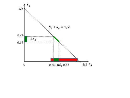
Figure 3: Projections of $\Delta S_{q}$ and $\Delta S_{g}$ on the line $S_{q}+S_{g}=1/2$ overlap, i.e. the values of $S_{q,g}$ of Eq. (35) within these intervals (green blocks) obey the requirement $S_{q}+S_{g}=1/2$.

IV Conclusions

We have demonstrated that the values of the parton helicities in the proton being calculated in DLA perfectly agree with the fact that the proton spin $=1/2$. In other words, the origin of the proton spin puzzle was the insufficient accuracy of the helicities description at small $x$.

In particular, using DGLAP or fixed-order calculations should have been complemented by resummation of DL corrections because the involved values of $x$ are small, $x\leq 0.05$, so DL terms dominate over other contributions.

The similar situation arises when the parton helicities are approximated by their small-$x$ asymptotics. The point is that the asymptotics reliably represent the parent amplitudes within their applicability region only, i.e. at $x\sim 10^{-5}$, whereas their values are small compared to the parent amplitudes outside the applicability region. For instance, the ratio $R_{as}=$ (Asymptotics of $g_{1}$)/$g_{1}$ plotted in Fig. 2 against $x$ drops when $x$ is getting smaller. Indeed, $R_{as}\approx 0.8$ at $x\sim 10^{-4}$ and $R_{as}\approx 0.6$ at $x\sim 10^{-3}$.

In the present paper we first have shown how to combine the RHIC data with the DL expressions for the helicities in order to get the straightforward solution of the problem in DLA. However, the helicities obtained in Refs. [31, 32] are represented by complicated expressions which are difficult to use. We postpone dealing with them for the future but for now we have suggested a shortcut by constructing the simple but realistic approximation for the quark and gluon helicities and obtained in Eq. (35) the tentative estimates of the parton helicities, which led to agreement with Eq. (1). Our results demonstrate that taking in consideration the Orbital Angular Momentum is not necessary for solving the proton spin problem.

V Acknowledgment

We are grateful to Yu.L. Kovchegov, M.A. Ivanov and S.M. Osipov for useful communications.

References

- [1] J. Ashman et. al., A measurement of the spin asymmetry and determination of the structure function g1 in deep inelastic muon-proton scattering, Physics Letters B 206 (1988) no. 2, 364.
- [2] J. Ashman et. al., An investigation of the spin structure of the proton in deep inelastic scattering of polarised muons on polarised protons, Nuclear Physics B 328. (1989) no. 1, 1.
- [3] C. A. Aidala, S. D. Bass, D. Hasch and G. K. Mallot, The Spin Structure of the Nucleon, Rev. Mod. Phys. 85 (2013) 655–691, [1209.2803].
- [4] A. Accardi et al., Electron Ion Collider: The Next QCD Frontier, Eur. Phys. J. A52 (2016) 268, [1212.1701].
- [5] E. Leader and C. Lorc´e, The angular momentum controversy: What’s it all about and does it matter?, Phys. Rept. 541 (2014) 163–248, [1309.4235].
- [6] E. C. Aschenauer et al., The RHIC Spin Program: Achievements and Future Opportunities, 1304.0079.
- [7] E.-C. Aschenauer et al., The RHIC SPIN Program: Achievements and Future Opportunities, 1501.01220.
- [8] D. Boer et al., Gluons and the quark sea at high energies: Distributions, polarization, tomography, 1108.1713.
- [9] A. Prokudin, Y. Hatta, Y. Kovchegov and C. Marquet, eds., Proceedings, Probing Nucleons and Nuclei in High Energy Collisions: Dedicated to the Physics of the Electron Ion Collider: Seattle (WA), United States, October 1 - November 16, 2018, WSP, 2020. 10.1142/11684.
- [10] X. Ji, F. Yuan and Y. Zhao, What we know and what we don’t know about the proton spin after 30 years, Nature Rev. Phys. 3 (2021) 27–38, [2009.01291].
- [11] R. Abdul Khalek et al., Science Requirements and Detector Concepts for the Electron-Ion Collider: EIC Yellow Report, 2103.05419.
- [12] R. L. Jaffe and A. Manohar, The G(1) Problem: Fact and Fantasy on the Spin of the Proton, Nucl. Phys. B337 (1990) 509.
- [13] X.-D. Ji, Gauge-Invariant Decomposition of Nucleon Spin, Phys. Rev. Lett. 78 (1997) 610, [hep-ph/9603249].
- [14] E. C. Aschenauer et. al., The RHIC Spin Program: Achievements and Future Opportunities, [arXiv:1304.0079 [nucl-ex]].
- [15] E. C. Aschenauer et. al., The RHIC SPIN Program: Achievements and Future Opportunities, [arXiv:1501.01220 [nucl-ex]].
- [16] Florian Cougoulic,1, Yuri V. Kovchegov, Andrey Tarasov and Yossathorn Tawabutr. Quark and Gluon Helicity Evolution at Small x: Revised and Updated. JHEP 07 (2022) 095.
- [17] Jeremy Borden and Yuri V. Kovchegov. Analytic Solution for the Revised Helicity Evolution at Small and Large : New Resummed Gluon-Gluon Polarized Anomalous Dimension and Intercept Phys.Rev.D 108 (2023) 1, 014001.
- [18] Daniel Adamiak, Yuri V. Kovchegov and Yossathorn Tawabutr. Helicity Evolution at Small : Revised Asymptotic Results at Large and Phys.Rev.D 108 (2023) 5, 5.
- [19] Yuri V. Kovchegov and Brandon Manley. Orbital angular momentum at small Revisited. JHEP 02 (2024) 060.
- [20] Renaud Boussarie, Yoshitaka Hatta, Feng Yuan. Proton Spin Structure at Small-x. Phys.Lett.B 797 (2019) 134817.
- [21] Yossathorn Tawabutr. eprint 2311.18185 [hep-ph].
- [22] Yuri V. Kovchegov, Daniel Pitonyak, Matthew D. Sivert. Helicity Evolution at Small : Flavor Singlet and Non-Singlet Observables Phys.Rev.D 95 (2017) 1, 014033.
- [23] Yuri V. Kovchegov, Daniel Pitonyak, Matthew D. Sivert. Small- asymptotics of the quark helicity distribution Phys.Rev.Lett. 118 (2017) 5, 052001.
- [24] Y. V. Kovchegov, D. Pitonyak and M. D. Sievert. Small- Asymptotics of the Gluon Helicity Distribution. JHEP 10 (2017) 198.
- [25] Y. V. Kovchegov and M. D. Sievert.Small- Helicity Evolution: an Operator Treatment Phys. Rev. D99 (2019) 054032.
- [26] Florian Cougoulic, Yuri V. Kovchegov. Helicity-dependent generalization of the JIMWLK evolution. Phys.Rev.D 100 (2019) 11, 114020.
- [27] Yuri V. Kovchegov, Andrey Tarasov, Yossathorn Tawabutr. Helicity evolution at small x: the single-logarithmic contribution. JHEP 03 (2022) 184.
- [28] F. Cougoulic, Y. V. Kovchegov, A. Tarasov and Y. Tawabutr. Quark and Gluon Helicity Evolution at Small x: Revised and Updated. JHEP 07 (2022) 095.
- [29] Jeremy Borden, Yuri V. Kovchegov. Analytic Solution for the Revised Helicity Evolution at Small x and Large Nc : New Resummed Gluon-Gluon Polarized Anomalous Dimension and Intercept. Phys.Rev.D 108 (2023) 1, 014001.
- [30] B.I. Ermolaev, M. Greco, S.I. Troyan. Intercepts of non-singlet structure functions. Nucl.Phys.B 594 (2001) 71.
- [31] B.I. Ermolaev, M. Greco, S.I. Troyan. Running coupling effects for the singlet structure function at small . Phys.Lett.B 579 (2004) 321.
- [32] B.I. Ermolaev, M. Greco, S.I. Troyan. Overview of the spin structure function at arbitrary and . Riv.Nuovo Cim. 33 (2010) 2, 57.
- [33] B.I. Ermolaev, M. Greco, S.I. Troyan. Comment on the recent COMPASS data on the spin structure function g(1). Eur.Phys.J.C 58 (2008) 29.
- [34] N.I. Kochelev, K. Lipka, W.D. Nowak, V. Vento, A.V. Vinnikov. Phys. Rev. D 67 (2003) 074014.