Self Supervised Correlation-based Permutations for Multi-View Clustering

Abstract

Fusing information from different modalities can enhance data analysis tasks, including clustering. However, existing multi-view clustering (MVC) solutions are limited to specific domains or rely on a suboptimal and computationally demanding two-stage procedure of representation and clustering. We propose an end-to-end deep learning-based MVC framework for general data (image, tabular, etc.). Our approach involves learning meaningful fused data representations with a novel permutation-based canonical correlation objective. Concurrently, we learn cluster assignments by identifying consistent pseudo-labels across multiple views. We demonstrate the effectiveness of our model using ten MVC benchmark datasets. Theoretically, we show that our model approximates the supervised linear discrimination analysis (LDA) representation. Additionally, we provide an error bound induced by false-pseudo label annotations.

1 Introduction

Clustering is a crucial technique in data-driven scientific discovery that helps to categorize samples into groups based on semantic relationships. This allows for a deeper understanding of complex datasets and is used in various domains such as gene expression analysis in Bioinformatics [1], efficient categorizing of large-scale medical images [2], and in collider physics [3]. Existing clustering approaches can be broadly categorized as centroid-based [4, 5, 6], density-based [7, 8, 9, 10], distribution-based [11, 12], hierarchical [13, 14] and deep learning model [15, 16]. Multi-view clustering is an extension of the clustering paradigm that simultaneously leverages diverse views of the same observations [17, 18, 19].

The main idea behind multi-view clustering is to combine information from multiple data facets (or views) to obtain a more comprehensive and accurate understanding of the underlying data structures. Each view may capture distinct aspects or facets of the data, and by integrating them, we can discover hidden patterns and relationships that might be obscured in any single view [20, 21]. This approach holds immense potential in various applications, from multimedia analysis [22] and bioinformatics [23] to social network analysis [24] and geophysics [25, 26].

Existing MVC methods can be divided into traditional (non-deep) and deep learning-based methods. Traditional MVC methods include: subspace methods [27, 28, 29], matrix factorization methods [30, 31, 32], and graph methods [33, 34, 35]. The main drawbacks of the traditional methods are poor representation ability, high computation complexity, and often limited performance in real-world data [36].

Recently, several deep learning-based MVC schemes have demonstrated promising representation and clustering capabilities [37, 38, 39, 40, 41, 42, 43]. Most of these methods adopt a two-stage approach, where they first learn representations, followed by clustering, as seen in works such as [44, 43, 37, 38, 39, 27, 45, 46, 47]. However, such a two-stage procedure can be computationally expensive and does not directly update the model’s weights based on cluster assignments; therefore, it may lead to suboptimal results.

A few studies presented an end-to-end scheme for MV representation learning and clustering [48, 49, 50, 51]). By performing both tasks simultaneously, MVC can improve the data embeddings by making them more suited for cluster assignments. However, the multi-view fusion process used in these studies may only be adaptable to some types of data, which can limit their generalization capabilities across a wide range of datasets.

We have introduced a new approach called COrrelation-based PERmutations (COPER) that aims to address the main challenges of multi-view clustering. Our deep learning model combines clustering and representation tasks, providing an end-to-end MVC framework for fusion and clustering. This eliminates the need for an additional step. The approach involves learning data representations with a novel self-supervision task. In this task, inter-class (within class) pseudo-labels are permuted (PER) across different views for canonical correlation (CO) analysis loss. The proposed framework maximizes intra-class (between class) variance and minimizes inter-class variation in the shared embedded space. Under mild assumptions, we demonstrate that our model approximates the same projection that would have been achieved by the (supervised) linear discriminant analysis (LDA) method [52].

Our main contributions are summarized as follows: (i) Develop a deep learning model that exploits self-supervision and a CCA-based objective for end-to-end MVC. (ii) Present a multi-view pseudo-labeling procedure for identifying consistent labels across views. (iii) Demonstrate empirically and theoretically that within cluster permutation can improve the usability of CCA-based representations for MVC. (iv) Analyze the relation between the solution of our new permutation-based CCA procedure and the solution of LDA. (v) Conduct an extensive experimental evaluation demonstrating our proposed model’s superiority over the state-of-the-art deep MVC models.

2 Related Work

Several existing MVC methods incorporate Deep Canonical correlation analysis (DCCA) during their representation learning phase. These methods obtain a useful representation by transforming multiple views into maximally correlated embeddings using nonlinear transformations [53, 54, 27, 47]. However, these methods use a suboptimal two-stage procedure, where the clustering scheme is applied to the representation learned through the CCA-based objective.

A few end-to-end, multi-view DCCA-based clustering solutions have been proposed; these include [48, 50], which update their representations to improve the clustering capabilities. Our model also falls under the same category of end-to-end representation learning and clustering. However, we have introduced some new elements that make our approach distinct from existing schemes. These include a new self-supervised permutation procedure that enhances the representation and a multi-view pseudo-label selection scheme. Empirical results demonstrate that these new components significantly improve clustering capabilities, presented in Section 6.

3 Background

3.1 Canonical Correlation Analysis (CCA)

Canonical Correlation Analysis (CCA) [55, 56] is a well-celebrated statistical framework for multi-view/modal representation learning. CCA can help analyze the associations between two sets of paired high-dimensional observations. This framework and its nonlinear [57, 58, 59, 60, 61, 62] or sparse [63, 64] extensions have been applied in various domains, including biology [65], neuroscience [66], medicine [67], and engineering [68].

The main goal of CCA is to find linear combinations of variables from each view, aiming to maximize their correlation. Formally, denoting the observations as ${\mbox{\boldmath$X$}}^{(1)}\in\mathbb{R}^{D_{1}\times N}$ and ${\mbox{\boldmath$X$}}^{(2)}\in\mathbb{R}^{D_{2}\times N}$, where both modalities are centered and encompass $N$ samples with $D_{1}$ and $D_{2}$ attributes, respectively. CCA seeks for canonical vectors ${\mbox{\boldmath$a$}}\in\mathbb{R}^{D_{1}}$ and ${\mbox{\boldmath$b$}}\in\mathbb{R}^{D_{2}}$ such that ${\mbox{\boldmath$u$}}={\mbox{\boldmath$a$}}^{T}{\mbox{\boldmath$X$}}^{(1)}$ and ${\mbox{\boldmath$v$}}={\mbox{\boldmath$b$}}^{T}{\mbox{\boldmath$X$}}^{(2)}$. The objective is to maximize correlations between these canonical variates, as represented by the following optimization:

$$\max_{{\mbox{\boldmath$a$}},{\mbox{\boldmath$b$}}\neq 0}\rho({\mbox{\boldmath$u$}},{\mbox{\boldmath$v$}})=\frac{{\mbox{\boldmath$a$}}^{T}{\mbox{\boldmath$X$}}^{(1)}({\mbox{\boldmath$X$}}^{(2)})^{T}{\mbox{\boldmath$b$}}}{\sqrt{{\mbox{\boldmath$a$}}^{T}{\mbox{\boldmath$X$}}({\mbox{\boldmath$X$}}^{(1)})^{T}{\mbox{\boldmath$a$}}}\sqrt{{\mbox{\boldmath$b$}}^{T}{\mbox{\boldmath$X$}}^{(2)}({\mbox{\boldmath$X$}}^{(2)})^{T}{\mbox{\boldmath$b$}}}}.$$

These canonical vectors can be found by solving the generalized eigenpair problem

$${C}_{1}^{-1} {C}_{12} {C}_{2}^{-1} {C}_{21} a = \lambda{\mbox{\boldmath$a$}}$$

$${C}_{2}^{-1} {C}_{21} {C}_{1}^{-1} {C}_{12} b = \lambda{\mbox{\boldmath$b$}}$$ (1)

where ${\mbox{\boldmath${C}_{1}$}},{\mbox{\boldmath${C}_{2}$}}$ are within view sample covariance matrices and ${\mbox{\boldmath${C}_{12}$}},{\mbox{\boldmath${C}_{21}$}}$ are cross-view sample covariance matrices.

Various extensions of CCA have been proposed to study non-linear relationships between the observed modalities. Some kernel-based methods, such as Kernel CCA [57], Non-parametric CCA [58], and Multi-view Diffusion maps [60, 61], explore non-linear connections within reproducing Hilbert spaces. However, these methods are limited by pre-defined kernels, have restricted interpolation capabilities, and do not scale well with large datasets.

To overcome these limitations [62] introduces Deep CCA (DCCA), which extends traditional CCA by leveraging deep neural networks to learn non-linear mappings between the input modalities automatically. This enables more flexible and scalable modeling of complex relationships in large datasets. In Section 4.3, we describe how we incorporate a DCCA objective to embed the multi-view data.

3.2 Self-Supervision for Clustering

Self-supervised learning is a technique for learning meaningful data representations without labeled observations. The main idea is to leverage information present in unlabeled samples to create a task that does not require any manual annotations. In clustering tasks, self-supervision improves data representation learning by assigning pseudo-labels to unlabeled data based on semantic similarities between samples. These pseudo-labels are then used to improve data representations through learning tasks.

In single-view data, two-stage clustering frameworks proposed by [69, 70, 71] alternate between clustering and using the cluster assignments as pseudo-labels to revise image representations. [72] have introduced a pseudo-labeling method that encourages the formation of more meaningful and coherent clusters that align with the semantic content of the images. Their framework treats some pseudo-labels as reliable, synergizing the similarity and discrepancy of the samples. For multi-view datasets, clustering and self-supervision frameworks [53, 38, 73] offer loss components that enforce consensus in the latent multi-view representations. We propose a new multi-view pseudo-labeling scheme that uses the labeled samples to define within-cluster permutations, which are used to enhance the learned embeddings.

4 The Proposed Method

4.1 Problem Setup

We are given a set of multi-view data $\mathcal{X}=\{{\mbox{\boldmath$X$}}^{(v)}\in\mathbb{R}^{d_{v}\times N}\}_{v=1}^{n_{v}}$ with $n_{v}$ views and $N$ samples. Each view is defined by ${\mbox{\boldmath$X$}}^{(v)}=[{\mbox{\boldmath$x$}}_{1}^{(v)},{\mbox{\boldmath$x$}}_{2}^{(v)},...,{\mbox{\boldmath$x$}}_{N}^{(v)}]$ and each ${\mbox{\boldmath$x$}}_{i}^{(v)}$ is a $d_{v}$-dimensional instance. Our objective is to predict cluster assignment $y_{i}$ for each tuple of instances $({\mbox{\boldmath$x$}}_{i}^{(1)},{\mbox{\boldmath$x$}}_{i}^{(2)},...,{\mbox{\boldmath$x$}}_{i}^{(n_{v})}),i=1,...,N$ in $\mathcal{X}$ and the number of clusters is $K$.

4.2 High Level Solution

At the core of our proposed solution are three components: (i) multi-view representation learning, (ii) reliable pseudo-label prediction, and (iii) within cluster sample permutations. These components are complementary and are trained in an end-to-end fashion based on multi-view observations.

Our representation learning component aims to create aligned data embedding by using a maximum correlation objective. This embedding captures the shared information across multiple views of the data. You can find more details in Section 4.3. The second component involves fusing the embeddings and predicting pseudo labels using a clustering head. We then present a filtration procedure to select reliable representatives in each cluster, which we describe in Section 4.4.

Our final component uses the selected representatives, which introduces random permutation to the samples from the same cluster across views. You can find the details of this permutation technique in Section 4.5. Through both theoretical and empirical analysis, we have shown that these permutations can enhance cluster separation when using CCA-based objectives. For more details, please see Sections 5.2 and 5.3. An overview of our model, called COPER, is presented in Fig. 1.

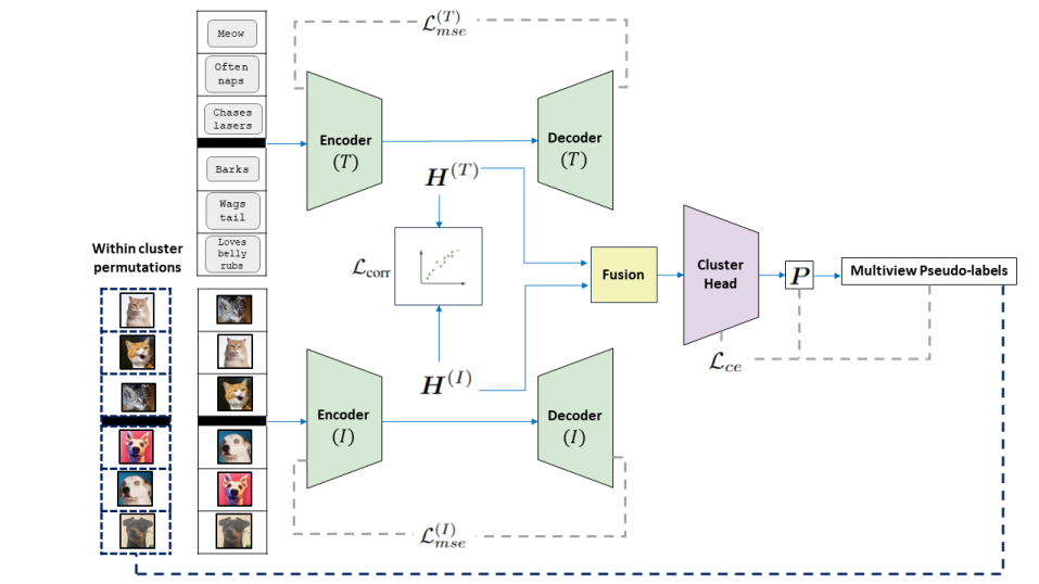
Figure 1: Our proposed deep learning model COPER. Illustration using two modalities, text (T) and image (I), are proceeded through view-specific auto-encoders, creating latent embeddings (${\mbox{\boldmath$H$}}^{(T)}$ and ${\mbox{\boldmath$H$}}^{(I)}$). These embeddings are aligned using a correlation loss and then fused to serve as input for the clustering head. The clustering head estimates a probability matrix P, which is used to obtain multi-view pseudo-labels. We then use this probability matrix along with the pseudo-labels to update the model weights through a cross-entropy loss. Finally, we generate within-cluster permutations based on these pseudo-labels, which help enhance the separation of clusters in the embedding space.

4.3 Deep Canonically Correlated Autoencoders

To learn meaningful representations from the multi-view observations, we use autoencoders equipped with a maximum correlation objective [54, 74]. Specifically, we train view-specific autoencoders $\mathcal{F}^{(v)}$ which extract latent representations $h_{i}^{(v)}$ and reconstruct $\hat{\mathbf{x}}_{i}^{(v)}$, where $\mathcal{F}^{(v)}(\mathbf{x}_{i}^{(v)})=(\mathbf{h}_{i}^{(v)},\hat{\mathbf{x}}_{i}^{(v)})$ for each sample $\mathbf{x}_{i}^{(v)}$ in view $v$. The model minimizes the mean squared error (MSE) by comparing reconstructed samples $\hat{\mathbf{x}}_{i}^{(v)}$ to the input $\mathbf{x}_{i}^{(v)}$:

$$\mathcal{L}_{mse}^{(v)}({\mbox{\boldmath$X$}}^{v})=\mathbb{E}_{\mathbf{x}_{i}^{(v)}\in\mathbf{X}^{(v)}}||\mathbf{x}_{i}^{(v)}-\hat{\mathbf{x}}_{i}^{(v)}||_{2}^{2}.$$

We use a correlation loss to force the embedding to be correlated (see Subsection 3.1). Denoting the latent representations by ${\mbox{\boldmath$H$}}^{(v)}\in\mathbb{R}^{d_{v}\times N}$, and ${\mbox{\boldmath$H$}}^{(w)}\in\mathbb{R}^{d_{w}\times N}$ generated by the autoencoders $\mathcal{F}^{(v)}$ and $\mathcal{F}^{(w)}$ respectively. The covariance matrix between these representations can be expressed as ${\mbox{\boldmath$C$}}_{vw}=\frac{1}{N-1}{\mbox{\boldmath$H$}}^{(v)}({\mbox{\boldmath$H$}}^{(w)})^{T}$. Similarly, the covariance matrices of ${\mbox{\boldmath$H$}}^{(v)}$ and ${\mbox{\boldmath$H$}}^{(w)}$ as ${\mbox{\boldmath$C$}}_{v}=\frac{1}{N-1}{\mbox{\boldmath$H$}}^{(v)}({\mbox{\boldmath$H$}}^{(v)})^{T}$ and ${\mbox{\boldmath$C$}}_{w}=\frac{1}{N-1}{\mbox{\boldmath$H$}}^{(w)}({\mbox{\boldmath$H$}}^{(w)})^{T}$. A negative trace expresses the correlation loss:

$$\mathcal{L}_{\text{corr}}({\mbox{\boldmath$H$}}^{(v)},{\mbox{\boldmath$H$}}^{(w)})=-\operatorname{Tr}\left[{\mbox{\boldmath$C$}}^{-1/2}_{w}{\mbox{\boldmath$C$}}_{wv}{\mbox{\boldmath$C$}}^{-1}_{v}{\mbox{\boldmath$C$}}_{vw}{\mbox{\boldmath$C$}}^{-1/2}_{w}\right].$$ (2)

4.4 Multi-view Pseudo-labeling

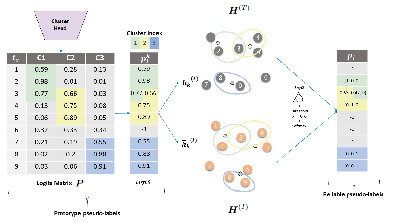
Figure 2: An illustration for our multi-view pseudo-labels scheme. The cluster head, denoted as $\mathcal{G}_{\Gamma}$, produces the matrix of logits values $P$. We choose the top three samples with the highest probabilities to create the prototype pseudo-labels for each cluster. In this particular example, the sample in the third index was assigned to two clusters. We then choose the reliable pseudo-labels as the top three examples that have the highest cosine similarity between the hidden representations, denoted as $\bar{{\mbox{\boldmath$h$}}}_{k}$. The reliable pseudo-labels are also filtered with a given threshold, $\lambda$. In addition, we use Softmax to create probabilities.

A key component of our model is a clustering head that predicts cluster assignments based on fused data embeddings. The predictions of the clustering head are then used for defining prototypes and reliable pseudo-labels, which will be exploited in the next step to improve the embedding by creating within cluster permutations (see Section 4.5.

The clustering head, denoted by $\mathcal{G}$, is optimized in a self-supervised manner along with the pseudo-labels introduced in this subsection. The clustering head accepts a fusion of latent embeddings represented by $\frac{1}{n_{v}}\sum_{v}{\mbox{\boldmath$H$}}^{(v)}$, and predicts cluster assignments represented by probability matrix, $\mathcal{G}(\frac{1}{n_{v}}\sum_{v}{\mbox{\boldmath$H$}}^{(v)})={\mbox{\boldmath$P$}}\in\mathbb{R}^{N\times K}$.

We now present the first part of our multi-view pseudo-labels scheme. For clarity and simplicity, we demonstrate this for a single view such that the notation for view $v$ is omitted in the rest of this section.

For each cluster in a given view, we select the top $\frac{N_{mb}}{K}$ probabilities in $P$ and use their index to get the prototype pseudo-labels samples ${\mbox{\boldmath$h$}}_{i}$ for cluster $k$:

$$\mathcal{T}_{k} =\{{\mbox{\boldmath$h$}}_{i}|i\in\text{argtopk}({\mbox{\boldmath$P$}}_{:,k},\frac{N_{mb}}{K}),$$

$$\quad\forall i=1,2,...,N_{mb}\},$$

where ${\mbox{\boldmath$P$}}_{:,k}$ denotes the $k$-th column of matrix $P$, $N_{mb}$ is the size of minibatch and $argtopk$ returns $\frac{N_{mb}}{K}$ most confident samples in ${\mbox{\boldmath$P$}}_{:,k}$. We now compute the cluster centers $\bar{{\mbox{\boldmath$h$}}}_{k}$ as the mean of samples in $\mathcal{T}_{k}$:

$$\bar{{\mbox{\boldmath$h$}}}_{k}=\frac{K}{N_{mb}}\sum_{{\mbox{\boldmath$h$}}_{i}\in\mathcal{T}_{k}}{\mbox{\boldmath$h$}}_{i}.$$ (3)

Next, we compute the cosine similarity between $\bar{{\mbox{\boldmath$h$}}}_{k}$ and every sample in ${\mbox{\boldmath$h$}}_{i}$. $\frac{N_{mb}}{K}$ of the most similar samples to $\bar{{\mbox{\boldmath$h$}}}_{k}$ are selected and are further filtered by passing the threshold $\lambda$, making them reliable pseudo-labels. This may lead to the possibility that a sample was assigned to more than one cluster. Assuming sample ${\mbox{\boldmath$x$}}_{i}$ was assigned to several clusters, we normalize the probabilities with softmax function: ${\mbox{\boldmath$\tilde{p_{i}}$}}=\frac{e^{p_{i}}}{\sum_{k}e^{p_{i}}}$, where ${p_{i}}=0.5\cdot(1+\frac{\bar{{\mbox{\boldmath$h$}}}_{k}\cdot{\mbox{\boldmath$h$}}_{i}}{||\bar{{\mbox{\boldmath$h$}}}_{k}||\cdot||{\mbox{\boldmath$h$}}_{i}||})$. We assign a corresponding one-hot vector representation if the sample was assigned with a single label. Samples with different pseudo-labels across views are filtered out, which leads to the same indices in all views. The set of indices that were assigned with reliable pseudo-labels is now denoted as ${\cal{I}}$.

We denote the pairs of samples and their pseudo-labels by $\mathcal{X}_{p}=\{({\mbox{\boldmath$x$}}_{i},{\mbox{\boldmath$\tilde{p_{i}}$}})\}_{i\in{\cal{I}}}$. The model $\mathcal{G}_{\Gamma}$ is now optimized with $\mathfrak{X}=\{\mathcal{X}_{p}\}_{v=1}^{n_{v}}$ by minimizing cross-entropy loss $\mathcal{L}_{ce}$ where $\mathcal{L}_{ce}$ is defined by:

$$\mathcal{L}_{ce}(\mathcal{X}_{p})=-\sum_{i\in{\cal{I}}}\tilde{p}_{i}\log(\tilde{p}_{i}).$$ (4)

4.5 Self-Supervised Canonical Correlation-based Permutations

We now discuss our core training phase, where samples with the same pseudo-labels are permuted within clusters across different pairs of views. This novel self-supervision task enhances intra-class scatter while attenuating inter-class variability of the latent embeddings. Further details, analysis, and examples are discussed in section  5.1.

First, we further process the samples and their pseudo-labels, $\mathfrak{X}$. Specifically, in case a sample is given more than one pseudo-label, we randomly select one of the pseudo-labels in ${\mbox{\boldmath$\tilde{p_{i}}$}}^{(v)}$, and the probabilities are changed to one-hot vector. Next, we filter out all samples not assigned to the same pseudo-labels across all views. The assigned pseudo-label for sample $i$ is denoted as $\hat{y_{i}}$. We now use these pseudo-labels to perform within cluster random permutations, which will enhance our representation and clustering capabilities.

Definition 4.1.

A random permutation for each view is defined for the vector of indices $\bar{{I}}_{k}\subseteq 1,...,N$ with pseudo labels for cluster $k$ as the application of the following operator $\Pi^{l}_{k}\bar{{I}}_{k}$, where $\Pi^{l}_{k}$ is randomly sampled from the set of all permutation matrices of size $\bar{N}_{k}\times\bar{N}_{k}$.

Here $\bar{{I}}_{k}$ are the $\bar{N}_{k}$ indices of samples assigned with pseudo-label $k$, and $l$ denotes the permutation index as different permutations may be applied several times. Once we apply these random permutations to samples across the different views ($v=1,...,n_{v}$), we create a new artificial correspondence between views in the dataset.

We denote the new permuted multi-view data as $\tilde{\mathfrak{X}}=\{\tilde{\mathcal{X}}_{p}^{(v)}\}_{v=1}^{n_{v}}$. The corresponding latent embedding are denoted as $\tilde{{\mbox{\boldmath$H$}}}^{(v)}$. All new permuted data is now used to train the model with cross-entropy loss as in Eq. 4 and correlation loss as in Eq. 2.

Overall our model is optimized using:

$$\begin{split}\mathcal{L}&=\sum_{v=1}^{n_{v}}[\mathcal{L}_{mse}^{(v)}+\mathcal{L}_{ce}^{(v)}]+\sum_{v=1}^{n_{v}}\sum_{w=v+1}^{n_{v}}\mathcal{L}_{\text{corr}}({\mbox{\boldmath$H$}}^{(v)},{\mbox{\boldmath$H$}}^{(w)}),\end{split}$$

where we apply all loss terms to both the original and permuted data in a similar way. This is done by selecting random batches and applying stochastic gradient descent (SGD). However, we have observed that when we feed samples from $\tilde{{\mbox{\boldmath$H$}}}^{(v)},\tilde{{\mbox{\boldmath$H$}}}^{(w)}$ to the correlation term, tuning its impact using the hyperparameter $\beta$ can lead to better performance. In Appendix section C.2, we present a procedure for tuning the hyperparameters of our model, and in Appendix section B we present the complexity analysis of our model.

5 Justification: COPER for Clustering

COPER relies on within-cluster random permutation to enhance the learned multiview embedding. The justification for this technique lies in two theoretical aspects. The first was presented by [75], which artificially created multi-view data by pairing examples with augmented samples from the same class. The authors then demonstrate that applying CCA to such data is equivalent to linear discriminant analysis (LDA) [52] (described in 5.1). Here, we show theoretically that within cluster permutations of multi-view data lead to similar results (see Section 5.2 and 5.3). This is also backed up by empirical evidence presented in Figure 3.

Chaudhuri et al. [76] presented an independent theoretical analysis that motivates our permutations. The authors showed that CCA-based objectives can improve cluster separation if the views are uncorrelated for samples within a given cluster. Our within-cluster permutations help obtain this property, as we demonstrate empirically in Figure 4.

5.1 Reminder: Linear Discriminant Analysis (LDA)

Fisher’s linear discriminant analysis (LDA) aims to preserve variance while seeking the optimal linear discriminant function [52]. Unlike unsupervised techniques such as principal component analysis (PCA) or canonical correlation analysis (CCA), LDA is a supervised method that incorporates categorical class label information to identify meaningful projections. The approach involves maximizing an objective function that takes into account the scatter properties of each class and the overall scatter. This objective function is constructed to be maximized through a projection that enhances intra-class scatter and diminishes inter-class scatter.

For a dataset ${\mbox{\boldmath$X$}}\in\mathbb{R}^{D\times N}$ and it’s covariance matrix $C$, we denote the inter-class covariance matrix as:

$${\mbox{\boldmath${C}_{e}$}}=\frac{1}{N}\sum_{k=1}^{K}\sum_{i=1}^{N_{k}}({\mbox{\boldmath$x$}}_{i}^{k}-{\mbox{\boldmath$\mu$}}_{k})({\mbox{\boldmath$x$}}_{i}^{k}-{\mbox{\boldmath$\mu$}}_{k})^{T}.$$

Where $N_{k}$ are the samples from class $k$, ${\mbox{\boldmath$x$}}_{i}^{k}$ is the $i$’th sample, and ${\mbox{\boldmath$\mu$}}_{k}$ is the mean. The inter-class covariance is:

$${\mbox{\boldmath${C}_{a}$}}=\sum_{k=1}^{K}\frac{N_{k}}{N}{\mbox{\boldmath$\mu$}}_{k}{{\mbox{\boldmath$\mu$}}_{k}}^{T},$$

and ${\mbox{\boldmath$C$}}={\mbox{\boldmath${C}_{e}$}}+{\mbox{\boldmath${C}_{a}$}}.$ The optimization for LDA can be formulated as:

$$\max_{{\mbox{\boldmath$h$}}\neq{\mbox{\boldmath$0$}}}\frac{{\mbox{\boldmath$h$}}^{T}{\mbox{\boldmath${C}_{a}$}}{\mbox{\boldmath$h$}}}{{\mbox{\boldmath$h$}}^{T}{\mbox{\boldmath${C}_{e}$}}{\mbox{\boldmath$h$}}}.$$

Which could be solved using a generalized eigenproblem:

$${\mbox{\boldmath${C}_{a}$}}{\mbox{\boldmath$h$}}=\lambda{\mbox{\boldmath${C}_{e}$}}{\mbox{\boldmath$h$}}$$

$${\mbox{\boldmath${C}_{e}^{-1}$}}{\mbox{\boldmath${C}_{a}$}}{\mbox{\boldmath$h$}}=\lambda{\mbox{\boldmath$h$}}.$$ (5)

In the following subsection, we show a connection between the solution of CCA with permutations induced within the cluster and the solution of LDA.

5.2 From COPER to LDA

In [75] the authors constructed an artificial multi-view setting by splitting samples into two views and pairing the views based on the class labels. Based on this procedure, they created an augmented multi-view dataset in which the shared information across views is the class label. They proved that applying CCA to such augmented data converges to the solution of LDA (described in Section 5.1).

We observe multi-view data and use the following assumption to prove a relation between our scheme and LDA:

Assumption 5.1.

For two different views $v,w$, the observations are created by some pushforward function (with noise) of some latent common parameter $\theta$ that is shared across the views. Specifically, ${\mbox{\boldmath$X$}}^{v}={\mbox{\boldmath$f$}}^{v}({\mbox{\boldmath$\theta$}},{\mbox{\boldmath$\epsilon$}}^{v})$ and ${\mbox{\boldmath$\epsilon$}}^{v}$ is view specific noise. The parameter $\theta$ carries the cluster information.

We note that assumptions about common latent variables were also used in prior work on CCA [77, 78]. Under this assumption, we show the following:

Proposition 5.2.

CCA with all inter-cluster permutation converges to the same representation extracted by LDA [52].

A proof of this proposition appears in Appendix  D.1, where we show that ${\mbox{\boldmath$h$}}_{LDA}={\mbox{\boldmath$h$}}_{CCA}$. The proof follows the analysis of [75]. Intuitively, this result indicates that the label information is leaked into embedding learned by CCA once we apply within cluster permutations. In Section 5.4, we conduct an experiment using Fashion MNIST to demonstrate how within cluster random permutation can enhance the embedding learned by CCA.

5.3 LDA Approximation

Since our model relies on pseudo-labels, these can induce errors in the random within-cluster permutation, influencing the learned representations. If such label errors are induced, Proposition 5.2 breaks and the solution of CCA with permutations is no longer equivalent to the solution of LDA.

To quantify this effect, we treat these induced errors as a perturbation matrix. We substitute ${C}_{e}^{-1}$${C}_{a}$ from Eq. 5 with $A$ and denote $D$ as the perturbation noise such that ${\mbox{\boldmath$\hat{A}$}}={\mbox{\boldmath$A$}}+{\mbox{\boldmath$D$}}$. In addition we use tools form perturbation theory [79] to provide the following upper bound for the approximated LDA eigenvalues:

$$|\hat{\lambda}_{i}-\lambda_{i}|\leq||{\mbox{\boldmath$D$}}||_{2},i=1\ldots n,$$ (6)

where $\lambda_{i}$ is the $i$’th LDA eigenvalue obtained from $A$; $\hat{\lambda}_{i}$ is the $i$’th LDA approximated eigenvalue obtained from $\hat{A}$; and $n$ is the total number of eigenvalues. In Appendix D.2, we provide a complete derivation of this approximation. In subsection 4.5, we conduct a controlled experiment to evaluate how label noise influences this approximation. This implies that the more the pseudo-labels resemble the ground truth labels, the closer the representation is to LDA. We presented empirical experiments in Section 5.4 to support this.

5.4 Case Study using Fashion MNIST

We conduct a controlled experiment using F-MNIST [80] to corroborate our theoretical results presented in this section. First, we create two coupled views by horizontally splitting the images. CCA is subsequently performed on the multi-view dataset, with different versions of within cluster sample permutations.

First, we only permute samples with the same label. We show in Fig. 3 (a) that such supervised permutations improve cluster separation, as evidenced by the increased ARI. Moreover, our experiments in panel (b) indicate that the CCA solution becomes more similar to the LDA solution. In panel (c), we have also confirmed our hypothesis that these permutations decrease the mean inter-class correlation across views (please refer to the second paragraph in Section 5 for more details). Next, we repeated the evaluations in panels (a) and (b) using permutations based on pseudo labels. We have also included the results based on random permutations and the original data (no permutation) as baselines. The results show that pseudo-label-based permutations also improve cluster separation and bring the representation of CCA closer to the solution of LDA.

We have conducted an experiment to measure the error induced by falsely annotated pseudo-labels. This experiment complements our LDA approximation presented in subsection  5.3. We first subsampled 20% of the data and then gradually introduced the remaining data with either real or noisy (false) labels. The results, as shown in Fig. 4, demonstrate that introducing false annotations increases the gap between the eigenvalues. On the other hand, adding more samples with correct annotations leads to the convergence of the solution to the full LDA solution.

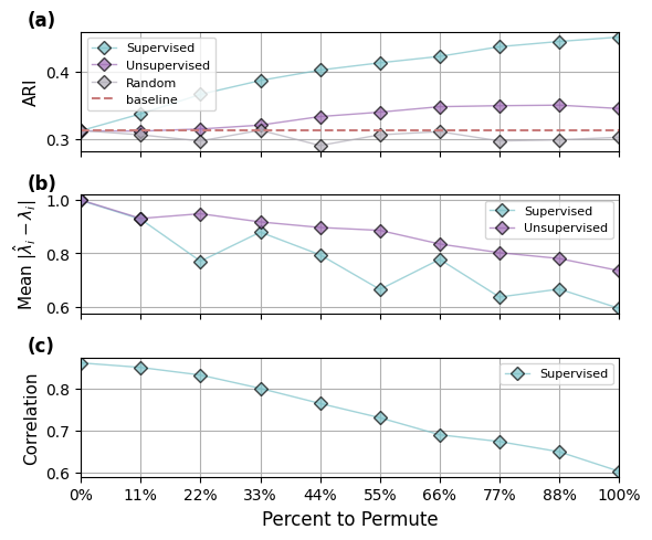
Figure 3: Case study of premutation CCA using Fashion MNIST. (a) Permuting more samples within a cluster improves cluster separation as measured by the Adjusted Rand Index (ARI). We compare labeled permutation (supervised) to pseudo-label-based (unsupervised) and random. (b) Permuting more samples also pushes the representation obtained by CCA towards LDA, as indicated by the gap between eigenvalues. (c) The mean inter-class correlation between views is attenuated as we permute more samples.

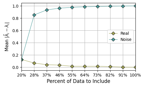
Figure 4: We conducted an experiment on LDA approximation with induced label noise. We gradually increased the number of samples from F-MNIST and analyzed the effect on the eigenvalues of LDA. We found that noisy annotations increase the eigenvalue gap compared to the full solution. In contrast, the addition of more real samples reduces the approximation error.

6 Real World Data

We conduct an extensive experiment with ten publicly available multi-view datasets used in recent works [51, 48]. The properties of the datasets are presented in Table 3, and a complete description appears in Appendix A. The implementation details are detailed in Appendix C.1

We assess the clustering performance with three commonly used metrics: Clustering Accuracy (ACC), The adjusted Rand index score (ARI), and Normalized Mutual Information (NMI). Both ACC and ARI are scored between 0 to 1, where higher values indicate better clustering performance. We conducted each experiment 10 times and reported the mean and standard deviation for each metric. We compare our model to DSMVC [48] and CVCL[51] and several two-stage baselines, where $K$-means was applied: Raw samples without any features transformations; PCA transformations; linear CCA transformations; Autoencoder (AE) transformations; Deep CCA with autoencoders (DCCA-AE) [54, 74] transformations.

We present the results in the Table 1. Our model outperforms state of the art models in both accuracy and the adjusted Rand index across all datasets, where the accuracy improvement reaches up to 14%. We note that the results of [51, 48] are different from the values reported by the authors since we report the mean over ten runs while they report the best result. We argue that our evaluation, which includes the standard deviation, provides a more informative indication of the capabilities of each method.

Table 1: Clustering results. Our model (COPER) is compared against two recent deep MVC models and two-stage $K$-Means clustering methods.

Method/Dataset	METABRIC	Reuters	Caltech101-20	VOC	Caltech5V-7	RBGD	MNIST-USPS	CCV	MSRVC1	Scene15
ACC
Raw	35.18$\pm$2.9	37.16$\pm$5.9	42.98$\pm$3.1	52.41$\pm$7.3	73.54$\pm$6.3	43.15$\pm$1.8	69.78$\pm$6.3	16.25$\pm$0.7	74.00$\pm$7.3	37.91$\pm$0.9
PCA	37.72$\pm$1.4	42.56$\pm$2.9	41.47$\pm$3.4	43.66$\pm$4.9	74.26$\pm$6.3	42.64$\pm$1.9	68.14$\pm$3.9	16.17$\pm$0.5	74.14$\pm$6.1	37.53$\pm$1.2
CCA	40.05$\pm$2.1	42.85$\pm$2.5	42.34$\pm$3.1	53.1$\pm$4.1	75.96$\pm$5.2	41.47$\pm$2.2	80.15$\pm$5	16.16$\pm$0.7	73.29$\pm$7.3	37.59$\pm$1.3
AE	38.92$\pm$2.5	43.35$\pm$4.0	40.39$\pm$2.3	36.66$\pm$2.69	54.48$\pm$3.2	32.16$\pm$1.6	33.83$\pm$3.6	15.58$\pm$0.6	56.76$\pm$3.8	33.59$\pm$2.3
DCCA-AE	45.39$\pm$2.8	43.18$\pm$2.8	48.18$\pm$3.4	46.53$\pm$2.7	58.37$\pm$3.9	32.59$\pm$1.3	92.19$\pm$2.4	18.28$\pm$0.9	56.76$\pm$3.8	33.70$\pm$2.0
DSMVC	40.60$\pm$3.8	46.37$\pm$4.4	39.33$\pm$2.4	57.82$\pm$5.0	79.24$\pm$9.5	39.77$\pm$3.6	70.06$\pm$10.3	17.90$\pm$1.2	60.71 $\pm$ 15.2	34.30 $\pm$ 2.9
CVCL	42.66$\pm$6.2	45.06$\pm$8.0	33.5$\pm$1.4	36.88$\pm$3.1	78.58$\pm$5.0	31.04$\pm$1.8	99.38$\pm$0.1	26.23$\pm$1.9	77.90 $\pm$ 12.3	40.16 $\pm$ 1.8
COPER	49.13$\pm$3.2	53.15 $\pm$ 3.3	54.83$\pm$3.9	64.65$\pm$2.6	82.81$\pm$5.1	49.80$\pm$0.8	99.88$\pm$0.0	28.06$\pm$1.1	89.14 $\pm$ 7.1	40.68 $\pm$ 1.6
ARI
Raw	18.64$\pm$1.2	7.49$\pm$7.7	34.58$\pm$4	29.51$\pm$7.4	57.19$\pm$5.9	24.13$\pm$1.2	58.88$\pm$4.8	5.45$\pm$0.3	58.53$\pm$5.8	22.31$\pm$0.4
PCA	19.05$\pm$1.5	19.88$\pm$1.4	31.75$\pm$3.5	21.44$\pm$5.1	57.91$\pm$4.7	23.78$\pm$1.4	54.55$\pm$2.8	5.45$\pm$0.2	58.39$\pm$5.9	22.0$\pm$0.4
CCA	19.84$\pm$1.7	18.76$\pm$1.7	32.68$\pm$3.8	34.69$\pm$5.4	60.01$\pm$1.9	24.59$\pm$1.7	71.09$\pm$4.5	5.32$\pm$0.3	56.97$\pm$7.2	22.57$\pm$0.5
AE	19.71$\pm$3.0	10.36$\pm$4.3	31.27$\pm$4.1	18.86$\pm$2.7	30.73$\pm$4.8	15.26$\pm$1.6	13.93$\pm$2.0	3.56$\pm$0.3	33.43$\pm$4.8	17.00$\pm$1.7
DCCA-AE	21.70$\pm$2.8	7.63$\pm$4.0	37.19$\pm$3.2	32.77$\pm$3.4	34.63$\pm$4.1	15.00$\pm$2.0	84.04$\pm$4.4	5.0$\pm$0.4	33.43$\pm$4.8	17.12$\pm$1.6
DSMVC	18.24$\pm$2.4	23.41$\pm$5.0	31.21$\pm$2.4	50.78$\pm$4.6	69.06$\pm$9.4	23.74$\pm$2.6	56.87$\pm$13.4	5.97$\pm$0.5	42.63 $\pm$ 19.0	18.85 $\pm$ 2.5
CVCL	22.69$\pm$4.3	22.39$\pm$8.8	24.85$\pm$0.9	22.49$\pm$2.7	63.25$\pm$6.3	16.16$\pm$1.3	98.63$\pm$0.2	12.72$\pm$1.3	64.27 $\pm$ 13.8	24.01 $\pm$ 1.7
COPER	26.77$\pm$2.4	22.80 $\pm$ 4.3	49.55$\pm$5.3	53.26$\pm$4.0	69.53$\pm$6.7	34.17$\pm$1.4	99.73$\pm$0.0	12.27$\pm$0.4	82.26 $\pm$ 9.0	25.00 $\pm$ 1.1
NMI
Raw	24.13$\pm$1.4	15.38$\pm$9.0	61.77$\pm$2.0	53.89$\pm$5.5	64.34$\pm$3.9	38.83$\pm$0.8	70.43$\pm$2.4	15.07$\pm$0.5	66.89$\pm$3.8	40.74$\pm$0.4
PCA	25.44$\pm$1.7	27.92$\pm$1.2	60.5$\pm$1.4	44.29$\pm$3.9	63.79$\pm$2.5	37.43$\pm$1.0	65.27$\pm$1.1	15.17$\pm$0.3	67.37$\pm$4.0	40.33$\pm$0.5
CCA	26.85$\pm$2.0	27.16$\pm$1.0	61.13$\pm$2.0	53.01$\pm$3.6	65.72$\pm$1.9	38.79$\pm$1.0	77.58$\pm$2.2	14.38$\pm$0.4	65.52$\pm$5.2	40.75$\pm$0.5
AE	27.34$\pm$2.6	18.61$\pm$3.2	50.15$\pm$2.4	30.46$\pm$2.0	38.97$\pm$5.2	28.85$\pm$1.4	22.83$\pm$2.5	10.68$\pm$1.0	48.31$\pm$4.0	33.18$\pm$2.6
DCCA-AE	30.95$\pm$2.8	23.04$\pm$3.1	54.46$\pm$2.4	47.29$\pm$4.0	43.38$\pm$3.9	27.54$\pm$3.5	85.32$\pm$3.3	16.39$\pm$1.0	48.31$\pm$4.0	33.65$\pm$2.0
DSMVC	25.51$\pm$1.9	29.48$\pm$4.8	60.72$\pm$1.4	65.13$\pm$3.2	75.08$\pm$6.8	37.60$\pm$2.5	67.80$\pm$11.5	16.70$\pm$0.9	57.77 $\pm$ 13.0	36.55 $\pm$ 3.3
CVCL	32.3$\pm$4.5	29.41$\pm$11.1	56.13$\pm$1.0	32.95$\pm$1.3	69.56$\pm$4.8	26.6$\pm$1.6	98.21$\pm$0.3	26.25$\pm$0.9	72.66 $\pm$ 8.9	41.13 $\pm$ 1.7
COPER	34.07$\pm$2.6	31.10 $\pm$ 4.1	49.25$\pm$6.2	58.54$\pm$2.2	74.03$\pm$4.6	38.13$\pm$0.9	99.64$\pm$0.1	26.32$\pm$0.7	86.15 $\pm$ 6.4	41.98 $\pm$ 1.2

6.1 Ablation Study

We performed an ablation to assess the impact of different components of our model. We created four variations of our model, each including different subsets of the components of COPER. These variations were: (i) only the multiple autoencoders (AE); (ii) COPER without pseudo-label predictions; (iii) COPER without within-cluster permutations; and (iv) COPER. For (i) and (ii), we utilized $K$-means to predict cluster assignments, as we no longer had a clustering head. We conducted this ablation study using the METABRIC dataset. In Table  2, we compare the clustering metrics across these variations of COPER. The results indicate that the pseudo-label procedure slightly improved assignment accuracy over $K$-means. Additionally, the new permutation scheme boosted performance by more than 10%.

Table 2: Ablation study on the METABRIC dataset.

Model	ACC	ARI	NMI
AE	38.92$\pm$2.5	19.71$\pm$3.0	27.34$\pm$2.6
COPER w/o pseudo-labels	45.39$\pm$2.8	21.70$\pm$2.8	30.95$\pm$2.8
COPER w/o permutations	45.82$\pm$3.2	22.41$\pm$3.3	22.41$\pm$31.3.1
COPER	49.13$\pm$2.9	26.77$\pm$2.4	34.07$\pm$2.6

6.2 Conclusion and Limitations

Our work presents a new approach called COrrelation-based PERmutations (COPER), a deep learning model for multi-view clustering (MVC). COPER integrates clustering and representation tasks into an end-to-end framework, eliminating the need for a separate clustering step. The model employs a unique self-supervision task, where inter-class pseudo-labels are permuted across views for canonical correlation analysis loss, contributing to the maximization of intra-class variance and minimization of inter-class variation in the shared embedded space.

We demonstrate that, under mild assumptions, our model approximates the projection achieved by the supervised linear discriminant analysis (LDA) method. Our contributions include the development of a self-supervised deep learning model for MVC, a multi-view pseudo-labeling procedure, empirical and theoretical insights into the efficacy of within-cluster permutation for canonical correlation analysis, an analytical examination of the relationship between our permutation-based CCA and LDA solutions, and an extensive experimental evaluation showing that our model can accurately cluster diverse data types.

It is important to acknowledge that our model has certain limitations. One of them is the potential requirement for relatively large batch sizes due to the DCCA loss. This is a known limitation of these types of objectives [62] and can be addressed by alternative objectives such as soft decorrelation [81]. Another limitation of our model is its sensitivity to datasets with many clusters. This is indicated by the results obtained on Caltech101-20 and CCV, which consist of 20 clusters, showing a smaller relative improvement. We note that the unweighted loss combination presented here is suboptimal. Evaluating smarter multitask schemes is an interesting topic for future work. Another direction for future work involves relaxing the requirement for bijective correspondence; this could be done by learning to match kernels as shown in [82].

6.3 Broader Impact

Our work presents a new deep learning-based solution for multi-view clustering, along with a theoretical foundation for its performance. This research can positively impact various domains by providing researchers and practitioners with a versatile data analysis tool for use across heterogeneous datasets, thereby facilitating advancements in knowledge discovery and decision-making processes. However, the proposed method has ethical implications and potential societal consequences that must be considered. It is crucial to pay attention to bias and fairness to prevent the amplification of biases across modalities. Transparency and explainability are essential to ensure user understanding and mitigate the perceived black-box nature of deep learning models.

Appendix A Datasets description

• METABRIC [83]: Consists of $1,440$ samples from breast cancer patients which are annotated by 8 subtypes based on InClust [84]. We observe tow modalities, namely the RNA gene expression data, and Copy Number Alteration (CNA) data. The dimensions of these modalities are $15,709$ and $47,127$ respectively.

• Reuters [85]: Consists of $18,758$ documents from $6$ different classes. Documents are represented as a bag of words, using a TFIDF-based weighting scheme. This dataset is a subset of the Reuters database, comprising the English version as well as translations in four distinct languages: French, German, Spanish, and Italian. Each language is treated as a different view. To further reduce the input dimensions we preprocess the data with a truncated version of $SVD$, turning all input dimentions to $3,000$.

• Caltech101-20 [30]: Consists of $2,386$ images of $20$ classes. This dataset is a subset of Caltech101. Each view is an extract handcrafted feature, including Gabor feature, Wavelet Moments, CENTRIST feature, HOG feature, GIST feature and LBP feature. .

• VOC [86]: Consists of $9,963$ image and text pairs from $20$ different classes. Following the conventions by [87, 88], $5,649$ instances are selected to construct a two-view dataset, where the first and the second view is 512 Gist features and 399 word frequency count of the instance respectively.

• Caltech-5V-7 [89]: Consists of $1,400$ images of $7$ classes. Same as Caltech101-20, this dataset is also a subset of Caltech101 and is comprised from the same views apart from the Gabor feature. ¹.

• RBGD [90]: Consists of $1,449$ samples of indoor scenes image-text of $13$ classes. We follow the version provided in [87, 91], where image features are extracted from a ResNet50 model pretrained on the ImageNet dataset and text features from a doc2vec model pretrained on the Wikipedia dataset.

• MNIST-USPS [92]: Consists of $5,000$ digits from $10$ different classes (digits). MNIST, and USPS are both handwritten digital datasets and are treated as two different views.

• CCV [93]: Consists of $6,773$ samples of indoor scenes image-text of $20$ classes. Flowing the convention in [39] we use the subset of the original CCV data. The views comprise of three hand-crafted features: STIP features with $5,000$ dimensional Bag-of-Words (BoWs) representation, SIFT features extracted every two seconds with $5,000$ dimensional BoWs representation, and MFCC features with $4,000$ dimensional BoWs.

• MSRCv1 Consists of 210 scene recognition images belonging to 7 categories [94]. Each image is described by 5 different types of features.

• Scene15 Consists of 4,485 scene images belonging to 15 classes [95].

Table 3: Datasets used in our experiments.

Dataset	# Samples	# Classes (K)	# Views	Dimensions	Ref
METABRIC	1440	8	2	[15709, 47127]	[83]
Reuters	18758	6	5	[3000] $\times$ 5	[85]
Caltech101-20	2386	20	6	[48, 40, 254, 1984, 512, 928]	[30]
VOC	5649	20	2	[512, 399]	[86]
Caltech-5V-7	1400	7	5	[40, 254, 1984, 512, 928]	[89]
RBGD	1449	13	2	[2048, 300]	[90]
MNIST-USPS	5000	10	2	[784, 784]	[92]
CCV	6773	20	3	[4000, 5000, 5000]	[93]
MSRVC1	210	7	5	[24, 576, 512, 256, 254]	[94]
Scene15	4485	15	3	[20, 59, 40]	[95]

Appendix B Complexity Analysis

Let $N_{mb}$ represent the number of samples in a mini batch and $N$ the total number of samples in the dataset, $L$ denote the maximum number of neurons in the model’s hidden layers across all views, and $l$ indicates the dimension of the low-dimensional embedding space. Additionally, $L^{\prime}$ stands for the number of neurons in the cluster head, and the number of clusters is denoted as $K$. For reliable labels, we denote $\widetilde{N}_{mb}$ as the number of samples in the permuted mini batch.

The time complexity of training each autoencoder is $\mathcal{O}(L\cdot N_{mb}\cdot\bigg{\lceil}\frac{N}{N_{mb}}\bigg{\rceil})$. With $M$ views, the total complexity for the pretraining phase is $\mathcal{O}(M\cdot L\cdot N\cdot\bigg{\lceil}\frac{N}{N_{mb}}\bigg{\rceil})$. Calculating the CCA loss for each pair of views has a complexity of $\mathcal{O}(N_{mb}^{2}\cdot\bigg{\lceil}\frac{N}{N_{mb}}\bigg{\rceil})$ for each pair. Since there are $\binom{M}{2}$ possible pairs, the total complexity for the CCA loss is $\mathcal{O}(M^{2}\cdot N_{mb}^{2}\cdot\bigg{\lceil}\frac{N}{N_{mb}}\bigg{\rceil})$.

The time complexity for training the cluster head is $\mathcal{O}(L^{\prime}\cdot N_{mb}\cdot\bigg{\lceil}\frac{N}{N_{mb}}\bigg{\rceil})$. Computing reliable labels for each view and each cluster also involves a complexity of $\mathcal{O}(M\cdot N_{mb}\cdot\bigg{\lceil}\frac{N}{N_{mb}}\bigg{\rceil}\cdot K)$. Therefore, the total complexity for the multi-view reliable labels tuning phase is $\mathcal{O}(M\cdot L^{\prime}\cdot N_{mb}\cdot\bigg{\lceil}\frac{N}{N_{mb}}\bigg{\rceil}\cdot K)$.

Computing CCA loss for reliable labels involves a complexity of $\mathcal{O}(\widetilde{N}_{mb}^{2}\cdot\bigg{\lceil}\frac{N}{\widetilde{N}_{mb}}\bigg{\rceil})$. The overall time complexity of our multi-view CCC model is the sum of the complexities of the individual phases. Therefore, the total time complexity is:

$$\mathcal{O}(M\cdot L\cdot N_{mb}\cdot\bigg{\lceil}\frac{N}{N_{mb}}\bigg{\rceil}+M^{2}\cdot N_{mb}^{2}\cdot\bigg{\lceil}\frac{N}{N_{mb}}\bigg{\rceil}+M\cdot L^{\prime}\cdot N_{mb}\cdot\bigg{\lceil}\frac{N}{N_{mb}}\bigg{\rceil}\cdot K+\widetilde{N}_{mb}^{2}\cdot\bigg{\lceil}\frac{N}{\widetilde{N}_{mb}}\bigg{\rceil}).$$

Where the dominant factor is:

$$\mathcal{O}(M^{2}\cdot N_{mb}^{2}\cdot\bigg{\lceil}\frac{N}{N_{mb}}\bigg{\rceil}).$$

Appendix C Experiments

C.1 Implementation Details

We implement our model using Pytorch, and the code is available for public use . All experiments were conducted using Nvidia A100 GPU server with Intel(R) Xeon(R) Gold 6338 CPU @ 2.00GHz.

C.2 Hyperparameters Tuning

To tune the parameters for each dataset, we utilize the Silhouette Coefficient [96] as an unsupervised metric for cluster separability. The Silhouette Coefficient is calculated using each sample’s mean intra-cluster distance and the mean nearest-cluster distance. The distances are calculated on the fusion of the learned representations $\frac{1}{n_{v}}\sum_{v}{\mbox{\boldmath$H$}}^{(v)}$. We calculate the Silhouette Coefficient after each epoch and pick the configuration that produces the maximal average Silhouette Coefficient value across a limited set of options. We present the correlation between Silhouette Coefficient value and clustering accuracy metrics in Table 4 on datasets VOC and METABRIC.

Table 4: Datasets used in our experiments.

Batch Size	ACC	ARI	NMI	Silhouette Coefficient
VOC
256	58.77	43.24	57.19	0.063
360	62.45	52.06	59.3	0.161
500	60.4	47.33	56.06	0.138
METABRIC
128	45.5	23.7	34.1	0.0396
256	53.9	27.8	37.7	0.0163
360	49.2	23.1	35.3	0.0569
500	46.4	27.9	38.9	0.1088

Appendix D Relation Between COPER and LDA

D.1 From COPER to LDA

$\mathcal{\theta}$ is treated as two different views $\mathcal{\theta}^{1}$ and $\mathcal{\theta}^{2}$ where each view is comprised of the same samples from $\mathcal{\theta}$ but different, inter-class permutation.

To create the views different permutations $\Pi^{l}$ of $\mathcal{\theta}$ for $l=0,1,2\dots,\infty$ are stacked, where the order of stacked permutations different for the two different views.

Lemma D.1.

Applying CCA on $\mathcal{\theta}^{1}$ and $\mathcal{\theta}^{2}$ produces the same projection as applying LDA on $\mathcal{\theta}$ with the (unknown) labels.

Since both $\mathcal{\theta}^{1}$ and $\mathcal{\theta}^{2}$ are comprised out of the same samples, it follows:

$${\mbox{\boldmath$C_{\mathcal{\theta}}$}}={\mbox{\boldmath$C_{\mathcal{\theta}^{1}}$}}={\mbox{\boldmath$C_{\mathcal{\theta}^{2}}$}}$$ (7)

And

$${\mbox{\boldmath$C_{\mathcal{\theta}^{1}\mathcal{\theta}^{2}}$}}={\mbox{\boldmath$C_{\mathcal{\theta}_{a}}$}}$$ (8)

We can use equations in  1 to find to solution for CCA:

$${\mbox{\boldmath$C_{\mathcal{\theta}}^{-1}$}}{\mbox{\boldmath$C_{\mathcal{\theta}_{a}}$}}{\mbox{\boldmath$C_{\mathcal{\theta}}^{-1}$}}{\mbox{\boldmath$C_{\mathcal{\theta}_{a}}$}}{\mbox{\boldmath$h$}}_{CCA}=\lambda_{CCA}{\mbox{\boldmath$h$}}_{CCA}$$ (9)

While from equation  5 we know that the solution for LDA is:

$${\mbox{\boldmath${C}_{a}$}}{\mbox{\boldmath$h$}}_{LDA}=\lambda_{LDA}{\mbox{\boldmath${C}_{e}$}}{\mbox{\boldmath$h$}}_{LDA}$$

We can further plug equation  5.1 and get:

$$\begin{split}&{\mbox{\boldmath${C}_{a}$}}{\mbox{\boldmath$h$}}_{LDA}=\lambda_{LDA}({\mbox{\boldmath${C}$}}-{\mbox{\boldmath${C}_{a}$}}){\mbox{\boldmath$h$}}_{LDA}\\ &\lambda_{LDA}({\mbox{\boldmath${C}$}}-{\mbox{\boldmath${C}_{a}$}}){\mbox{\boldmath$h$}}_{LDA}=\lambda_{LDA}{\mbox{\boldmath${C}$}}{\mbox{\boldmath$h$}}_{LDA}-\lambda_{LDA}{\mbox{\boldmath${C}_{a}$}}{\mbox{\boldmath$h$}}_{LDA}\\ &(1+\lambda_{LDA}){\mbox{\boldmath${C}_{a}$}}{\mbox{\boldmath$h$}}_{LDA}=\lambda_{LDA}{\mbox{\boldmath${C}$}}{\mbox{\boldmath$h$}}_{LDA}\\ &{\mbox{\boldmath${C}_{a}$}}{\mbox{\boldmath$h$}}_{LDA}=\frac{\lambda_{LDA}}{1+\lambda_{LDA}}{\mbox{\boldmath${C}$}}{\mbox{\boldmath$h$}}_{LDA}\\ &{\mbox{\boldmath${C}^{-1}$}}{\mbox{\boldmath${C}_{a}$}}{\mbox{\boldmath$h$}}_{LDA}=\frac{\lambda_{LDA}}{1+\lambda_{LDA}}{\mbox{\boldmath$h$}}_{LDA}\end{split}$$

Next, if we substitute ${\mbox{\boldmath${C}^{-1}$}}{\mbox{\boldmath${C}_{a}$}}=A$ and $\frac{\lambda_{LDA}}{1+\lambda_{LDA}}=\lambda^{*}$ in  D.1 we get :

$$A{\mbox{\boldmath$h$}}_{LDA}=\lambda^{*}{\mbox{\boldmath$h$}}_{LDA}$$ (10)

In addition if we substitute this in  9 we get:

$$\begin{split}&{\mbox{\boldmath$C_{\mathcal{\theta}}^{-1}$}}{\mbox{\boldmath$C_{\mathcal{\theta}_{a}}$}}{\mbox{\boldmath$C_{\mathcal{\theta}}^{-1}$}}{\mbox{\boldmath$C_{\mathcal{\theta}_{a}}$}}h_{CCA}=AAh_{CCA}\\ &AAh_{CCA}=A(A{\mbox{\boldmath$h$}}_{CCA})\\ &A(A{\mbox{\boldmath$h$}}_{CCA})=A(\lambda^{*}{\mbox{\boldmath$h$}}_{LDA})\\ &A(\lambda^{*}{\mbox{\boldmath$h$}}_{LDA})=\lambda^{*}(A{\mbox{\boldmath$h$}}_{LDA})\\ &\lambda^{*}(A{\mbox{\boldmath$h$}}_{LDA})=\lambda^{*}(\lambda^{*}{\mbox{\boldmath$h$}}_{LDA})\\ &\lambda^{*}(\lambda^{*}{\mbox{\boldmath$h$}}_{LDA})=\lambda_{CCA}{\mbox{\boldmath$h$}}_{CCA}\\ \end{split}$$

Since the canonical correlation coefficients are the square root of the eigenvalue obtained from the generalized eigenvalue problem it follows that ${\mbox{\boldmath$h$}}_{LDA}={\mbox{\boldmath$h$}}_{CCA}$

D.2 LDA Approximation

First, to simplify notation, we denoted $h$ and $\hat{h}$ the LDA representation and our representation which is based on pseudo-labels that are potentially incorrect. In the previous sections we saw that $\hat{{\mbox{\boldmath$C$}}}_{\mathcal{\theta}}^{-1}$ and $\hat{C}_{{\mathcal{\theta}}_{a}}$ are used compute $h$ in equation  5.1. Hence, to assess this equivalence, we draw attention to potential errors in estimating $\hat{{\mbox{\boldmath$C$}}}_{\mathcal{\theta}}$ from equation  7, where ${\mbox{\boldmath$\hat{C}_{\mathcal{\theta}}$}}={\mbox{\boldmath$\hat{C}_{{\mathcal{\theta}}_{e}}$}}+{\mbox{\boldmath$\hat{C}_{{\mathcal{\theta}}_{a}}$}}$.

Let $\hat{N_{k}}$ be the estimated samples for each class $k$, and $\hat{{\mbox{\boldmath$\mu$}}}_{k}$ it’s estimated mean. $\bar{N}_{k}$ are the indices of samples from class $k$ not included in $\hat{N_{k}}$. $\tilde{N}_{k}$ are samples not in class $k$, which are incorrectly included in $\hat{N_{k}}$, and $\ddot{N}_{k}$ are samples in $\hat{N_{k}}$ which are correctly included, the corresponding class for samples in $\ddot{N}_{k}$ are assumed to be known for this analysis.

For ${\mbox{\boldmath$\hat{C}$}}_{{\mathcal{\theta}}_{e}}=\frac{1}{N_{mb}}\sum_{k=1}^{K}({\mbox{\boldmath$x$}}_{i}^{k}-\hat{{\mbox{\boldmath$\mu$}}}_{k})({\mbox{\boldmath$x$}}_{i}^{k}-\hat{{\mbox{\boldmath$\mu$}}}_{k})^{T}$, Incomplete inclusion of all inter-class samples may cause error. As this depends on the batch size and the pseudo-labels batch size. We denote this type of error as:

$${\mbox{\boldmath$E$}}^{1}=-\frac{1}{\sum_{k=1}^{K}|\bar{N}_{k}|}\sum_{k=1}^{K}\sum_{\begin{subarray}{c}i\in\bar{N}_{k}\end{subarray}}({\mbox{\boldmath$x$}}_{i}^{k}-\hat{{\mbox{\boldmath$\mu$}}}_{k})({\mbox{\boldmath$x$}}_{i}^{k}-\hat{{\mbox{\boldmath$\mu$}}}_{k})^{T}.$$

In addition, false pseudo-labels cause samples from different classes to be permuted together. We denote this type of error as:

$${\mbox{\boldmath$E$}}^{2} =\frac{1}{\sum_{k=1}^{K}|\tilde{N}_{k}||\ddot{N}_{k}|}\sum_{k=1}^{K}\sum_{\begin{subarray}{c}i\in\ddot{N}_{k}\end{subarray}}\sum_{\begin{subarray}{c}j\in\tilde{N}_{k}\end{subarray}}({\mbox{\boldmath$x$}}_{i}^{k}-\hat{{\mbox{\boldmath$\mu$}}}_{k})({\mbox{\boldmath$x$}}_{j}^{q}-\hat{{\mbox{\boldmath$\mu$}}}_{q})^{T}.$$

where $q$ is the true class of samples $j$.

For ${\mbox{\boldmath${\hat{C}}_{\mathcal{\theta}_{a}}$}}=\frac{\hat{N}_{k}}{N_{mb}}\sum_{k=1}^{K}\hat{{\mbox{\boldmath$\mu$}}}_{k}({\hat{\mu}_{k}})^{T}$. Errors in estimating $\hat{\mu}_{k}$, denoted by $\Delta{\mbox{\boldmath$\mu$}}_{k}={\mbox{\boldmath$\mu$}}_{k}-\hat{{\mbox{\boldmath$\mu$}}}_{k}$ can be further propagated to the third type of error, denoted as:

$${\mbox{\boldmath$E$}}^{3}=-\frac{\hat{N}_{k}}{N_{mb}}\Delta{\mbox{\boldmath$\mu$}}_{k}(\Delta{\mbox{\boldmath$\mu$}}_{k})^{T}$$

Together all three types of errors can be expressed as ${\mbox{\boldmath$E$}}:={\mbox{\boldmath$E$}}^{1}+{\mbox{\boldmath$E$}}^{2}+{\mbox{\boldmath$E$}}^{3}$:

Taking these errors into account we can now treat them as a perturbations. Formally:

$$\begin{split}&{\mbox{\boldmath${\hat{C}}_{{\mathcal{\theta}}_{a}}$}}={\mbox{\boldmath${C}_{{\mathcal{\theta}}_{a}}$}}+{\mbox{\boldmath$E$}}^{3}\\ &{\mbox{\boldmath${\hat{C}}_{{\mathcal{\theta}}_{e}}$}}={\mbox{\boldmath${C}_{{\mathcal{\theta}}_{e}}$}}+{\mbox{\boldmath$E$}}^{1}+{\mbox{\boldmath$E$}}^{2}\\ &{\mbox{\boldmath${\hat{C}}_{{\mathcal{\theta}}}$}}={\mbox{\boldmath${C}_{{\mathcal{\theta}}}$}}+{\mbox{\boldmath$E$}}\end{split}$$

Since the latent dimension is significantly smaller than the input dimension, it is plausible to assume that ${\hat{C}}_{{\mathcal{\theta}}}$ is invertible. In addition, we express the first order approximation of the inverse as:

$${\mbox{\boldmath${\hat{C}}_{{\mathcal{\theta}}}^{-1}$}}=({\mbox{\boldmath${C}_{{\mathcal{\theta}}}$}}+{\mbox{\boldmath$E$}})^{-1}\\ ={\mbox{\boldmath${C}_{{\mathcal{\theta}}}^{-1}$}}-{\mbox{\boldmath${C}_{{\mathcal{\theta}}}^{-1}$}}{\mbox{\boldmath$E$}}{\mbox{\boldmath${C}_{{\mathcal{\theta}}}^{-1}$}}\\$$

This is accurate up to terms of order $||E||^{2}$ [79].

This means that the estimated matrix $A$ from Eq.  10, $\hat{{\mbox{\boldmath$A$}}}$ can be written as:

$$\begin{split}&\hat{A}={\mbox{\boldmath${\hat{C}}_{{\mathcal{\theta}}}^{-1}$}}{\mbox{\boldmath${\hat{C}}_{{\mathcal{\theta}}_{a}}$}}\\ &{\mbox{\boldmath${\hat{C}}_{{\mathcal{\theta}}}^{-1}$}}{\mbox{\boldmath${\hat{C}}_{{\mathcal{\theta}}_{a}}$}}=({\mbox{\boldmath${C}_{{\mathcal{\theta}}}^{-1}$}}-{\mbox{\boldmath${C}_{{\mathcal{\theta}}}^{-1}$}}{\mbox{\boldmath$E$}}{\mbox{\boldmath${C}_{{\mathcal{\theta}}}^{-1}$}})({\mbox{\boldmath${C}_{{\mathcal{\theta}}_{a}}$}}+{\mbox{\boldmath$E$}}^{3})\\ &({\mbox{\boldmath${C}_{{\mathcal{\theta}}}^{-1}$}}-{\mbox{\boldmath${C}_{{\mathcal{\theta}}}^{-1}$}}{\mbox{\boldmath$E$}}{\mbox{\boldmath${C}_{{\mathcal{\theta}}}^{-1}$}})({\mbox{\boldmath${C}_{{\mathcal{\theta}}_{a}}$}}+{\mbox{\boldmath$E$}}^{3})=({\mbox{\boldmath${C}_{{\mathcal{\theta}}}^{-1}$}}-{\mbox{\boldmath${C}_{{\mathcal{\theta}}}^{-1}$}}{\mbox{\boldmath$E$}}{\mbox{\boldmath${C}_{{\mathcal{\theta}}}^{-1}$}})({\mbox{\boldmath${C}_{{\mathcal{\theta}}}$}}-{\mbox{\boldmath${C}_{{\mathcal{\theta}}_{e}}$}}+{\mbox{\boldmath$E$}}^{3})\\ &({\mbox{\boldmath${C}_{{\mathcal{\theta}}}^{-1}$}}-{\mbox{\boldmath${C}_{{\mathcal{\theta}}}^{-1}$}}{\mbox{\boldmath$E$}}{\mbox{\boldmath${C}_{{\mathcal{\theta}}}^{-1}$}})({\mbox{\boldmath${C}_{{\mathcal{\theta}}}$}}-{\mbox{\boldmath${C}_{{\mathcal{\theta}}_{e}}$}}+{\mbox{\boldmath$E$}}^{3})={\mbox{\boldmath${C}_{{\mathcal{\theta}}}^{-1}$}}{\mbox{\boldmath${C}_{{\mathcal{\theta}}}$}}-{\mbox{\boldmath${C}_{{\mathcal{\theta}}}^{-1}$}}{\mbox{\boldmath$E$}}{\mbox{\boldmath${C}_{{\mathcal{\theta}}}^{-1}$}}{\mbox{\boldmath${C}_{{\mathcal{\theta}}}$}}-\\ &\quad{\mbox{\boldmath${C}_{{\mathcal{\theta}}}^{-1}$}}{\mbox{\boldmath${C}_{{\mathcal{\theta}}_{e}}$}}+{\mbox{\boldmath${C}_{{\mathcal{\theta}}}^{-1}$}}{\mbox{\boldmath$E$}}{\mbox{\boldmath${C}_{{\mathcal{\theta}}}^{-1}$}}{\mbox{\boldmath${C}_{{\mathcal{\theta}}_{e}}$}}+{\mbox{\boldmath${C}_{{\mathcal{\theta}}}^{-1}$}}{\mbox{\boldmath$E$}}^{3}-{\mbox{\boldmath${C}_{{\mathcal{\theta}}}^{-1}$}}{\mbox{\boldmath$E$}}{\mbox{\boldmath${C}_{{\mathcal{\theta}}}^{-1}$}}{\mbox{\boldmath$E$}}^{3}\\ &{\mbox{\boldmath${C}_{{\mathcal{\theta}}}^{-1}$}}{\mbox{\boldmath${C}_{{\mathcal{\theta}}}$}}-{\mbox{\boldmath${C}_{{\mathcal{\theta}}}^{-1}$}}{\mbox{\boldmath$E$}}{\mbox{\boldmath${C}_{{\mathcal{\theta}}}^{-1}$}}{\mbox{\boldmath${C}_{{\mathcal{\theta}}}$}}-{\mbox{\boldmath${C}_{{\mathcal{\theta}}}^{-1}$}}{\mbox{\boldmath${C}_{{\mathcal{\theta}}_{e}}$}}+\\ &\quad{\mbox{\boldmath${C}_{{\mathcal{\theta}}}^{-1}$}}{\mbox{\boldmath$E$}}{\mbox{\boldmath${C}_{{\mathcal{\theta}}}^{-1}$}}{\mbox{\boldmath${C}_{{\mathcal{\theta}}_{e}}$}}+{\mbox{\boldmath${C}_{{\mathcal{\theta}}}^{-1}$}}{\mbox{\boldmath$E$}}^{3}-{\mbox{\boldmath${C}_{{\mathcal{\theta}}}^{-1}$}}{\mbox{\boldmath$E$}}{\mbox{\boldmath${C}_{{\mathcal{\theta}}}^{-1}$}}{\mbox{\boldmath$E$}}^{3}=\\ &\quad{\mbox{\boldmath$I$}}-{\mbox{\boldmath${C}_{{\mathcal{\theta}}}^{-1}$}}{\mbox{\boldmath$E$}}{\mbox{\boldmath$I$}}-{\mbox{\boldmath${C}_{{\mathcal{\theta}}}^{-1}$}}{\mbox{\boldmath${C}_{{\mathcal{\theta}}_{e}}$}}+{\mbox{\boldmath${C}_{{\mathcal{\theta}}}^{-1}$}}{\mbox{\boldmath$E$}}{\mbox{\boldmath${C}_{{\mathcal{\theta}}}^{-1}$}}{\mbox{\boldmath${C}_{{\mathcal{\theta}}_{e}}$}}+{\mbox{\boldmath${C}_{{\mathcal{\theta}}}^{-1}$}}{\mbox{\boldmath$E$}}^{3}-{\mbox{\boldmath${C}_{{\mathcal{\theta}}}^{-1}$}}{\mbox{\boldmath$E$}}{\mbox{\boldmath${C}_{{\mathcal{\theta}}}^{-1}$}}{\mbox{\boldmath$E$}}^{3}\end{split}$$

And $A$ can be expressed as:

$$\begin{split}&{\mbox{\boldmath$A$}}={\mbox{\boldmath${C}_{{\mathcal{\theta}}}^{-1}$}}{\mbox{\boldmath${C}_{{\mathcal{\theta}}_{a}}$}}\\ &{\mbox{\boldmath${C}_{{\mathcal{\theta}}}^{-1}$}}{\mbox{\boldmath${C}_{{\mathcal{\theta}}_{a}}$}}={\mbox{\boldmath${C}_{{\mathcal{\theta}}}^{-1}$}}({\mbox{\boldmath${C}_{{\mathcal{\theta}}}$}}-{\mbox{\boldmath${C}_{{\mathcal{\theta}_{e}}}$}})\\ &{\mbox{\boldmath${C}_{{\mathcal{\theta}}}^{-1}$}}({\mbox{\boldmath${C}_{{\mathcal{\theta}}}$}}-{\mbox{\boldmath${C}_{{\mathcal{\theta}_{e}}}$}})={\mbox{\boldmath${C}_{{\mathcal{\theta}}}^{-1}$}}{\mbox{\boldmath${C}_{{\mathcal{\theta}}}$}}-{\mbox{\boldmath${C}_{{\mathcal{\theta}}}^{-1}$}}{\mbox{\boldmath${C}_{{\mathcal{\theta}_{e}}}$}}\\ &{\mbox{\boldmath${C}_{{\mathcal{\theta}}}^{-1}$}}{\mbox{\boldmath${C}_{{\mathcal{\theta}}}$}}-{\mbox{\boldmath${C}_{{\mathcal{\theta}}}^{-1}$}}{\mbox{\boldmath${C}_{{\mathcal{\theta}_{e}}}$}}={\mbox{\boldmath$I$}}-{\mbox{\boldmath${C}_{{\mathcal{\theta}}}^{-1}$}}{\mbox{\boldmath${C}_{{\mathcal{\theta}_{e}}}$}}\\ \end{split}$$

Now we can estimate the perturbation from $A$, denoted as $D$:

$$\begin{split}&{\mbox{\boldmath$D$}}={\mbox{\boldmath$A$}}-{\mbox{\boldmath$\hat{A}$}}\\ &{\mbox{\boldmath$A$}}-{\mbox{\boldmath$\hat{A}$}}=({\mbox{\boldmath$I$}}-{\mbox{\boldmath${C}_{{\mathcal{\theta}}}^{-1}$}}{\mbox{\boldmath${C}_{{\mathcal{\theta}_{e}}}$}})-({\mbox{\boldmath$I$}}-{\mbox{\boldmath${C}_{{\mathcal{\theta}}}^{-1}$}}{\mbox{\boldmath$E$}}{\mbox{\boldmath$I$}}-{\mbox{\boldmath${C}_{{\mathcal{\theta}}}^{-1}$}}{\mbox{\boldmath${C}_{{\mathcal{\theta}}_{e}}$}}+{\mbox{\boldmath${C}_{{\mathcal{\theta}}}^{-1}$}}{\mbox{\boldmath$E$}}{\mbox{\boldmath${C}_{{\mathcal{\theta}}}^{-1}$}}{\mbox{\boldmath${C}_{{\mathcal{\theta}}_{e}}$}}+{\mbox{\boldmath${C}_{{\mathcal{\theta}}}^{-1}$}}{\mbox{\boldmath$E$}}^{3}-{\mbox{\boldmath${C}_{{\mathcal{\theta}}}^{-1}$}}{\mbox{\boldmath$E$}}{\mbox{\boldmath${C}_{{\mathcal{\theta}}}^{-1}$}}{\mbox{\boldmath$E$}}^{3})\\ &({\mbox{\boldmath$I$}}-{\mbox{\boldmath${C}_{{\mathcal{\theta}}}^{-1}$}}{\mbox{\boldmath${C}_{{\mathcal{\theta}_{e}}}$}})-({\mbox{\boldmath$I$}}-{\mbox{\boldmath${C}_{{\mathcal{\theta}}}^{-1}$}}{\mbox{\boldmath$E$}}{\mbox{\boldmath$I$}}-{\mbox{\boldmath${C}_{{\mathcal{\theta}}}^{-1}$}}{\mbox{\boldmath${C}_{{\mathcal{\theta}}_{e}}$}}+{\mbox{\boldmath${C}_{{\mathcal{\theta}}}^{-1}$}}{\mbox{\boldmath$E$}}{\mbox{\boldmath${C}_{{\mathcal{\theta}}}^{-1}$}}{\mbox{\boldmath${C}_{{\mathcal{\theta}}_{e}}$}}+{\mbox{\boldmath${C}_{{\mathcal{\theta}}}^{-1}$}}{\mbox{\boldmath$E$}}^{3}-{\mbox{\boldmath${C}_{{\mathcal{\theta}}}^{-1}$}}{\mbox{\boldmath$E$}}{\mbox{\boldmath${C}_{{\mathcal{\theta}}}^{-1}$}}{\mbox{\boldmath$E$}}^{3})=\\ &\quad{\mbox{\boldmath${C}_{{\mathcal{\theta}}}^{-1}$}}{\mbox{\boldmath$E$}}-{\mbox{\boldmath${C}_{{\mathcal{\theta}}}^{-1}$}}{\mbox{\boldmath$E$}}{\mbox{\boldmath${C}_{{\mathcal{\theta}}}^{-1}$}}{\mbox{\boldmath${C}_{{\mathcal{\theta}}_{e}}$}}-{\mbox{\boldmath${C}_{{\mathcal{\theta}}}^{-1}$}}{\mbox{\boldmath$E$}}^{3}+{\mbox{\boldmath${C}_{{\mathcal{\theta}}}^{-1}$}}{\mbox{\boldmath$E$}}{\mbox{\boldmath${C}_{{\mathcal{\theta}}}^{-1}$}}{\mbox{\boldmath$E$}}^{3}\end{split}$$

This perturbation can be used as bound for the approximated eigenvalues according to [79]:

$$|\hat{\lambda}_{i}-\lambda_{i}|\leq||{\mbox{\boldmath$D$}}||_{2},i=1\ldots n$$ (11)

References

- Armingol et al. [2021] Erick Armingol, Adam Officer, Olivier Harismendy, and Nathan E Lewis. Deciphering cell–cell interactions and communication from gene expression. Nature Reviews Genetics, 22(2):71–88, 2021.
- Kart et al. [2021] Turkay Kart, Wenjia Bai, Ben Glocker, and Daniel Rueckert. Deepmcat: large-scale deep clustering for medical image categorization. In Deep Generative Models, and Data Augmentation, Labelling, and Imperfections: First Workshop, DGM4MICCAI 2021, and First Workshop, DALI 2021, Held in Conjunction with MICCAI 2021, Strasbourg, France, October 1, 2021, Proceedings 1, pages 259–267. Springer, 2021.
- Mikuni and Canelli [2021] Vinicius Mikuni and Florencia Canelli. Unsupervised clustering for collider physics. Physical Review D, 103(9):092007, 2021.
- Boley et al. [1999] Daniel Boley, Maria Gini, Robert Gross, Eui-Hong Sam Han, Kyle Hastings, George Karypis, Vipin Kumar, Bamshad Mobasher, and Jerome Moore. Partitioning-based clustering for web document categorization. Decision Support Systems, 27(3):329–341, 1999.
- Jain [2010] Anil K Jain. Data clustering: 50 years beyond k-means. Pattern recognition letters, 31(8):651–666, 2010.
- Velmurugan and Santhanam [2011] T Velmurugan and T Santhanam. A survey of partition based clustering algorithms in data mining: An experimental approach. Information Technology Journal, 10(3):478–484, 2011.
- Januzaj et al. [2004] Eshref Januzaj, Hans-Peter Kriegel, and Martin Pfeifle. Scalable density-based distributed clustering. In Knowledge Discovery in Databases: PKDD 2004: 8th European Conference on Principles and Practice of Knowledge Discovery in Databases, Pisa, Italy, September 20-24, 2004. Proceedings 8, pages 231–244. Springer, 2004.
- Kriegel and Pfeifle [2005] Hans-Peter Kriegel and Martin Pfeifle. Density-based clustering of uncertain data. In Proceedings of the eleventh ACM SIGKDD international conference on Knowledge discovery in data mining, pages 672–677, 2005.
- Chen and Tu [2007] Yixin Chen and Li Tu. Density-based clustering for real-time stream data. In Proceedings of the 13th ACM SIGKDD international conference on Knowledge discovery and data mining, pages 133–142, 2007.
- Duan et al. [2007] Lian Duan, Lida Xu, Feng Guo, Jun Lee, and Baopin Yan. A local-density based spatial clustering algorithm with noise. Information systems, 32(7):978–986, 2007.
- Preheim et al. [2013] Sarah P Preheim, Allison R Perrotta, Antonio M Martin-Platero, Anika Gupta, and Eric J Alm. Distribution-based clustering: using ecology to refine the operational taxonomic unit. Applied and environmental microbiology, 79(21):6593–6603, 2013.
- Jiang et al. [2011a] Bin Jiang, Jian Pei, Yufei Tao, and Xuemin Lin. Clustering uncertain data based on probability distribution similarity. IEEE Transactions on Knowledge and Data Engineering, 25(4):751–763, 2011a.
- Murtagh [1983] Fionn Murtagh. A survey of recent advances in hierarchical clustering algorithms. The computer journal, 26(4):354–359, 1983.
- Carlsson et al. [2010] Gunnar E Carlsson, Facundo Mémoli, et al. Characterization, stability and convergence of hierarchical clustering methods. J. Mach. Learn. Res., 11(Apr):1425–1470, 2010.
- Svirsky and Lindenbaum [2023] Jonathan Svirsky and Ofir Lindenbaum. Interpretable deep clustering. arXiv preprint arXiv:2306.04785, 2023.
- Rozner et al. [2023] Amit Rozner, Barak Battash, Lior Wolf, and Ofir Lindenbaum. Domain-generalizable multiple-domain clustering. arXiv preprint arXiv:2301.13530, 2023.
- Sun and Tao [2014] Xiaoshuai Sun and Dacheng Tao. A survey of multiview machine learning. Neurocomputing, 128:22–45, 2014.
- Kumar et al. [2011] Ankit Kumar, Hal Daumé III, and Amol Saha. Co-regularized multi-view spectral clustering. Proceedings of the 28th international conference on machine learning (ICML-11), pages 521–528, 2011.
- Li et al. [2018a] Xiang Li, Xiaojie Guo, and Zhi Zhang. Multiview clustering: A survey. In 2018 24th International Conference on Pattern Recognition (ICPR), pages 387–392. IEEE, 2018a.
- Huang et al. [2012] Xudong Huang, Yanan Gu, Kang Liu, and Xudong Gao. A self-training co-training algorithm for multiview spectral clustering. Pattern Recognition Letters, 33(13):1690–1700, 2012.
- Xu et al. [2013] Chang Xu, Dacheng Tao, and Chao Xu. A survey on multi-view learning. arXiv preprint arXiv:1304.5634, 2013.
- Li et al. [2017] Zhenguo Li, Hongke Zhao, Ke Lu, and Dacheng Tao. Multimodal clustering and content-based fusion for multimedia analysis. In 2017 IEEE International Conference on Multimedia and Expo (ICME), pages 1–6. IEEE, 2017.
- Xu et al. [2014] Zhongping Xu, Dacheng Tao, Chao Xu, and Jie Yang. A survey of multi-view representation learning. Neurocomputing, 128:27–42, 2014.
- Cao et al. [2015a] Xin Cao, Chang Yu, and Jiebo Luo. Diversified multi-view video recommendation. IEEE Transactions on Multimedia, 17(4):511–525, 2015a.
- Lindenbaum et al. [2019] Ofir Lindenbaum, Neta Rabin, Yuri Bregman, and Amir Averbuch. Seismic event discrimination using deep cca. IEEE Geoscience and Remote Sensing Letters, 17(11):1856–1860, 2019.
- Lindenbaum et al. [2018] Ofir Lindenbaum, Yuri Bregman, Neta Rabin, and Amir Averbuch. Multiview kernels for low-dimensional modeling of seismic events. IEEE Transactions on Geoscience and Remote Sensing, 56(6):3300–3310, 2018.
- Cao et al. [2015b] Xiaochun Cao, Changqing Zhang, Huazhu Fu, Si Liu, and Hua Zhang. Diversity-induced multi-view subspace clustering. In CVPR, pages 586–594, 2015b.
- Luo et al. [2018] Shirui Luo, Changqing Zhang, Wei Zhang, and Xiaochun Cao. Consistent and specific multi-view subspace clustering. In AAAI, 2018.
- Li et al. [2019a] Ruihuang Li, Changqing Zhang, Huazhu Fu, Xi Peng, Tianyi Zhou, and Qinghua Hu. Reciprocal multi-layer subspace learning for multi-view clustering. In ICCV, pages 8172–8180, 2019a.
- Zhao et al. [2017] Handong Zhao, Zhengming Ding, and Yun Fu. Multi-view clustering via deep matrix factorization. In AAAI, pages 2921–2927, 2017.
- Wen et al. [2018] Jie Wen, Zheng Zhang, Yong Xu, and Zuofeng Zhong. Incomplete multi-view clustering via graph regularized matrix factorization. In ECCV Workshops, 2018.
- Yang et al. [2021] Zuyuan Yang, Naiyao Liang, Wei Yan, Zhenni Li, and Shengli Xie. Uniform distribution non-negative matrix factorization for multiview clustering. IEEE Transactions on Cybernetics, pages 3249–3262, 2021.
- Nie et al. [2017] Feiping Nie, Jing Li, and Xuelong Li. Self-weighted multiview clustering with multiple graphs. In IJCAI, pages 2564–2570, 2017.
- Zhan et al. [2017] Kun Zhan, Changqing Zhang, Junpeng Guan, and Junsheng Wang. Graph learning for multiview clustering. IEEE Transactions on Cybernetics, 48(10):2887–2895, 2017.
- Zhu et al. [2018] Xiaofeng Zhu, Shichao Zhang, Wei He, Rongyao Hu, Cong Lei, and Pengfei Zhu. One-step multi-view spectral clustering. IEEE Transactions on Knowledge and Data Engineering, 31(10):2022–2034, 2018.
- Guo and Ye [2019] Jun Guo and Jiahui Ye. Anchors bring ease: An embarrassingly simple approach to partial multi-view clustering. In AAAI, pages 118–125, 2019.
- Abavisani and Patel [2018] Mahdi Abavisani and Vishal M Patel. Deep multimodal subspace clustering networks. IEEE Journal of Selected Topics in Signal Processing, 12(6):1601–1614, 2018.
- Alwassel et al. [2019] Humam Alwassel, Dhruv Mahajan, Bruno Korbar, Lorenzo Torresani, Bernard Ghanem, and Du Tran. Self-supervised learning by cross-modal audio-video clustering. In NeurIPS, pages 9758–9770, 2019.
- Li et al. [2019b] Zhaoyang Li, Qianqian Wang, Zhiqiang Tao, Quanxue Gao, and Zhaohua Yang. Deep adversarial multi-view clustering network. In IJCAI, pages 2952–2958, 2019b.
- Yin et al. [2020] Ming Yin, Weitian Huang, and Junbin Gao. Shared generative latent representation learning for multi-view clustering. In AAAI, pages 6688–6695, 2020.
- Wen et al. [2020] Jie Wen, Zheng Zhang, Yong Xu, Bob Zhang, Lunke Fei, and Guo-Sen Xie. CDIMC-net: Cognitive deep incomplete multi-view clustering network. In IJCAI, pages 3230–3236, 2020.
- Xu et al. [2021a] Jie Xu, Yazhou Ren, Guofeng Li, Lili Pan, Ce Zhu, and Zenglin Xu. Deep embedded multi-view clustering with collaborative training. Information Sciences, 573:279–290, 2021a.
- Xu et al. [2021b] Jie Xu, Yazhou Ren, Huayi Tang, Xiaorong Pu, Xiaofeng Zhu, Ming Zeng, and Lifang He. Multi-VAE: Learning disentangled view-common and view-peculiar visual representations for multi-view clustering. In ICCV, pages 9234–9243, 2021b.
- Lin et al. [2021] Yijie Lin, Yuanbiao Gou, Zitao Liu, Boyun Li, Jiancheng Lv, and Xi Peng. COMPLETER: Incomplete multi-view clustering via contrastive prediction. In CVPR, 2021.
- Zhang et al. [2017a] Changqing Zhang, Qinghua Hu, Huazhu Fu, Pengfei Zhu, and Xiaochun Cao. Latent multi-view subspace clustering. In CVPR, pages 4279–4287, 2017a.
- Brbić and Kopriva [2018] Maria Brbić and Ivica Kopriva. Multi-view low-rank sparse subspace clustering. Pattern Recognition, 73:247–258, 2018.
- Tang et al. [2018] Xiaoliang Tang, Xuan Tang, Wanli Wang, Li Fang, and Xian Wei. Deep multi-view sparse subspace clustering. In Proceedings of the 2018 VII International Conference on Network, Communication and Computing, pages 115–119, 2018.
- Tang and Liu [2022] Huayi Tang and Yong Liu. Deep safe multi-view clustering: Reducing the risk of clustering performance degradation caused by view increase. In Proceedings of the IEEE/CVF Conference on Computer Vision and Pattern Recognition, pages 202–211, 2022.
- Trosten et al. [2021a] Daniel J. Trosten, Sigurd Løkse, Robert Jenssen, and Michael Kampffmeyer. Reconsidering representation alignment for multi-view clustering. In CVPR, pages 1255–1265, 2021a.
- Chen et al. [2020] Mansheng Chen, Ling Huang, Chang-Dong Wang, and Dong Huang. Multi-view clustering in latent embedding space. In AAAI, pages 3513–3520, 2020.
- Chen et al. [2023] Jie Chen, Hua Mao, Wai Lok Woo, and Xi Peng. Deep multiview clustering by contrasting cluster assignments. In Proceedings of the IEEE/CVF International Conference on Computer Vision (ICCV), pages 16752–16761, October 2023.
- Fisher [1936] Ronald A Fisher. The use of multiple measurements in taxonomic problems. Annals of eugenics, 7(2):179–188, 1936.
- Xin et al. [2021] Bowen Xin, Shan Zeng, and Xiuying Wang. Self-supervised deep correlational multi-view clustering. In 2021 International Joint Conference on Neural Networks (IJCNN), pages 1–8. IEEE, 2021.
- Chandar et al. [2016] Sarath Chandar, Mitesh M Khapra, Hugo Larochelle, and Balaraman Ravindran. Correlational neural networks. Neural computation, 28(2):257–285, 2016.
- Harold [1936] Hotelling Harold. Relations between two sets of variables. Biometrika, 28(3):321–377, 1936.
- Thompson [1984] Bruce Thompson. Canonical correlation analysis: Uses and interpretation. Number 47. Sage, 1984.
- Bach and Jordan [2002] Francis R Bach and Michael I Jordan. Kernel independent component analysis. Journal of machine learning research, 3(Jul):1–48, 2002.
- Michaeli et al. [2016] Tomer Michaeli, Weiran Wang, and Karen Livescu. Nonparametric canonical correlation analysis. In International conference on machine learning, pages 1967–1976. PMLR, 2016.
- Lindenbaum et al. [2015] Ofir Lindenbaum, Arie Yeredor, and Moshe Salhov. Learning coupled embedding using multiview diffusion maps. In Latent Variable Analysis and Signal Separation: 12th International Conference, LVA/ICA 2015, Liberec, Czech Republic, August 25-28, 2015, Proceedings 12, pages 127–134. Springer, 2015.
- Lindenbaum et al. [2020] Ofir Lindenbaum, Arie Yeredor, Moshe Salhov, and Amir Averbuch. Multi-view diffusion maps. Information Fusion, 55:127–149, 2020.
- Salhov et al. [2020] Moshe Salhov, Ofir Lindenbaum, Yariv Aizenbud, Avi Silberschatz, Yoel Shkolnisky, and Amir Averbuch. Multi-view kernel consensus for data analysis. Applied and Computational Harmonic Analysis, 49(1):208–228, 2020.
- Andrew et al. [2013] Galen Andrew, Raman Arora, Jeff Bilmes, and Karen Livescu. Deep canonical correlation analysis. In ICML, pages 1247–1255, 2013.
- Lindenbaum et al. [2021] Ofir Lindenbaum, Moshe Salhov, Amir Averbuch, and Yuval Kluger. L0-sparse canonical correlation analysis. In International Conference on Learning Representations, 2021.
- Yan et al. [2023] Weiqing Yan, Yuanyang Zhang, Chenlei Lv, Chang Tang, Guanghui Yue, Liang Liao, and Weisi Lin. Gcfagg: Global and cross-view feature aggregation for multi-view clustering. In Proceedings of the IEEE/CVF Conference on Computer Vision and Pattern Recognition, pages 19863–19872, 2023.
- Pimentel et al. [2018] Harold Pimentel, Zhiyue Hu, and Haiyan Huang. Biclustering by sparse canonical correlation analysis. Quantitative Biology, 6:56–67, 2018.
- Al-Shargie et al. [2017] Fares Al-Shargie, Tong Boon Tang, and Masashi Kiguchi. Assessment of mental stress effects on prefrontal cortical activities using canonical correlation analysis: an fnirs-eeg study. Biomedical optics express, 8(5):2583–2598, 2017.
- Zhang et al. [2017b] Yu Zhang, Guoxu Zhou, Jing Jin, Yangsong Zhang, Xingyu Wang, and Andrzej Cichocki. Sparse bayesian multiway canonical correlation analysis for eeg pattern recognition. Neurocomputing, 225:103–110, 2017b.
- Chen et al. [2017] Zhiwen Chen, Steven X Ding, Tao Peng, Chunhua Yang, and Weihua Gui. Fault detection for non-gaussian processes using generalized canonical correlation analysis and randomized algorithms. IEEE Transactions on Industrial Electronics, 65(2):1559–1567, 2017.
- Caron et al. [2018] Mathilde Caron, Piotr Bojanowski, Armand Joulin, and Matthijs Douze. Deep clustering for unsupervised learning of visual features. In Proceedings of the European conference on computer vision (ECCV), pages 132–149, 2018.
- Caron et al. [2020] Mathilde Caron, Ishan Misra, Julien Mairal, Priya Goyal, Piotr Bojanowski, and Armand Joulin. Unsupervised learning of visual features by contrasting cluster assignments. Advances in neural information processing systems, 33:9912–9924, 2020.
- Nousi and Tefas [2020] Paraskevi Nousi and Anastasios Tefas. Self-supervised autoencoders for clustering and classification. Evolving Systems, 11(3):453–466, 2020.
- Niu et al. [2022] Chuang Niu, Hongming Shan, and Ge Wang. Spice: Semantic pseudo-labeling for image clustering. IEEE Transactions on Image Processing, 31:7264–7278, 2022.
- Li et al. [2018b] Chao Li, Cheng Deng, Ning Li, Wei Liu, Xinbo Gao, and Dacheng Tao. Self-supervised adversarial hashing networks for cross-modal retrieval. In Proceedings of the IEEE conference on computer vision and pattern recognition, pages 4242–4251, 2018b.
- Wang et al. [2015] Weiran Wang, Raman Arora, Karen Livescu, and Jeff Bilmes. On deep multi-view representation learning. In ICML, pages 1083–1092, 2015.
- Kursun et al. [2011] Olcay Kursun, Ethem Alpaydin, and Oleg V Favorov. Canonical correlation analysis using within-class coupling. Pattern Recognition Letters, 32(2):134–144, 2011.
- Chaudhuri et al. [2009] Kamalika Chaudhuri, Sham M Kakade, Karen Livescu, and Karthik Sridharan. Multi-view clustering via canonical correlation analysis. In Proceedings of the 26th annual international conference on machine learning, pages 129–136, 2009.
- Benton et al. [2017] Adrian Benton, Huda Khayrallah, Biman Gujral, Dee Ann Reisinger, Sheng Zhang, and Raman Arora. Deep generalized canonical correlation analysis. arXiv preprint arXiv:1702.02519, 2017.
- Lyu and Fu [2020] Qi Lyu and Xiao Fu. Nonlinear multiview analysis: Identifiability and neural network-assisted implementation. IEEE Transactions on Signal Processing, 68:2697–2712, 2020.
- Stewart and Sun [1990] Gilbert W Stewart and Ji-guang Sun. Matrix perturbation theory. (No Title), 1990.
- Xiao et al. [2017] Han Xiao, Kashif Rasul, and Roland Vollgraf. Fashion-mnist: a novel image dataset for benchmarking machine learning algorithms. arXiv preprint arXiv:1708.07747, 2017.
- Chang et al. [2018] Xiaobin Chang, Tao Xiang, and Timothy M Hospedales. Scalable and effective deep cca via soft decorrelation. In Proceedings of the IEEE Conference on Computer Vision and Pattern Recognition, pages 1488–1497, 2018.
- Yampolsky et al. [2023] Tamir Baruch Yampolsky, Ronen Talmon, and Ofir Lindenbaum. Domain and modality adaptation using multi-kernel matching. In 2023 31st European Signal Processing Conference (EUSIPCO), pages 1285–1289. IEEE, 2023.
- Curtis et al. [2012] Christina Curtis, Sohrab P Shah, Suet-Feung Chin, Gulisa Turashvili, Oscar M Rueda, Mark J Dunning, Doug Speed, Andy G Lynch, Shamith Samarajiwa, Yinyin Yuan, et al. The genomic and transcriptomic architecture of 2,000 breast tumours reveals novel subgroups. Nature, 486(7403):346–352, 2012.
- Dawson et al. [2013] Sarah-Jane Dawson, Oscar M Rueda, Samuel Aparicio, and Carlos Caldas. A new genome-driven integrated classification of breast cancer and its implications. The EMBO journal, 32(5):617–628, 2013.
- Amini et al. [2009] Massih R Amini, Nicolas Usunier, and Cyril Goutte. Learning from multiple partially observed views-an application to multilingual text categorization. Advances in neural information processing systems, 22, 2009.
- Everingham et al. [2010] Mark Everingham, Luc Van Gool, Christopher KI Williams, John Winn, and Andrew Zisserman. The pascal visual object classes (voc) challenge. International journal of computer vision, 88:303–338, 2010.
- Trosten et al. [2021b] Daniel J Trosten, Sigurd Lokse, Robert Jenssen, and Michael Kampffmeyer. Reconsidering representation alignment for multi-view clustering. In Proceedings of the IEEE/CVF conference on computer vision and pattern recognition, pages 1255–1265, 2021b.
- Van der Maaten and Hinton [2008] Laurens Van der Maaten and Geoffrey Hinton. Visualizing data using t-sne. Journal of machine learning research, 9(11), 2008.
- Dueck and Frey [2007] Delbert Dueck and Brendan J Frey. Non-metric affinity propagation for unsupervised image categorization. In 2007 IEEE 11th international conference on computer vision, pages 1–8. IEEE, 2007.
- Kong et al. [2014] Chen Kong, Dahua Lin, Mohit Bansal, Raquel Urtasun, and Sanja Fidler. What are you talking about? text-to-image coreference. In Proceedings of the IEEE conference on computer vision and pattern recognition, pages 3558–3565, 2014.
- Zhou and Shen [2020] Runwu Zhou and Yi-Dong Shen. End-to-end adversarial-attention network for multi-modal clustering. In CVPR, pages 14619–14628, 2020.
- Asuncion and Newman [2007] Arthur Asuncion and David Newman. Uci machine learning repository, 2007.
- Jiang et al. [2011b] Yu-Gang Jiang, Guangnan Ye, Shih-Fu Chang, Daniel Ellis, and Alexander C Loui. Consumer video understanding: A benchmark database and an evaluation of human and machine performance. In ICMR, pages 1–8, 2011b.
- Zhao et al. [2020] Wei Zhao, Cai Xu, Ziyu Guan, and Ying Liu. Multiview concept learning via deep matrix factorization. IEEE transactions on neural networks and learning systems, 32(2):814–825, 2020.
- Fei-Fei and Perona [2005] Li Fei-Fei and Pietro Perona. A bayesian hierarchical model for learning natural scene categories. In 2005 IEEE Computer Society Conference on Computer Vision and Pattern Recognition (CVPR’05), volume 2, pages 524–531. IEEE, 2005.
- Rousseeuw [1987] Peter J Rousseeuw. Silhouettes: a graphical aid to the interpretation and validation of cluster analysis. Journal of computational and applied mathematics, 20:53–65, 1987.