Where Do We Go from Here? Multi-scale Allocentric Relational Inference
from Natural Spatial Descriptions
Abstract
When communicating routes in natural language, the concept of acquired spatial knowledge is crucial for geographic information retrieval (GIR) and in spatial cognitive research. However, NLP navigation studies often overlook the impact of such acquired knowledge on textual descriptions. Current navigation studies concentrate on egocentric local descriptions (e.g., ‘it will be on your right’) that require reasoning over the agent’s local perception. These instructions are typically given as a sequence of steps, with each action-step explicitly mentioning and being followed by a landmark that the agent can use to verify they are on the right path (e.g., ‘turn right and then you will see...’). In contrast, descriptions based on knowledge acquired through a map provide a complete view of the environment and capture its overall structure. These instructions (e.g., ‘it is south of Central Park and a block north of a police station’) are typically non-sequential, contain allocentric relations, with multiple spatial relations and implicit actions, without any explicit verification. This paper introduces the Rendezvous (RVS) task and dataset, which includes 10,404 examples of English geospatial instructions for reaching a target location using map-knowledge. Our analysis reveals that RVS exhibits a richer use of spatial allocentric relations, and requires resolving more spatial relations simultaneously compared to previous text-based navigation benchmarks.11footnotetext: This work was done partly during an internship at Google Research.222Data and code: https://github.com/OnlpLab/RVS.
1 Introduction
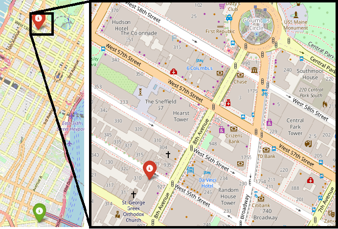
In today’s world, cell phones with powerful mapping applications are widely used. However, even with this technology at our fingertips, many people still rely on geospatial instructions to arrange rendezvous locations by providing natural language descriptions that reference landmarks and their geospatial relation, e.g., ‘...a block north of a police station’ (Figure 1). Retrieving locations and paths from natural language spatial descriptions is essential for disaster areas Hu et al. (2023), for the billions of people without addresses UPU (2012); Abebrese (2019), and for Geographic Information Retrieval (GIR), especially from the web (Spink et al., 2002; Sanderson and Kohler, 2004).
In spatial cognitive research, it is widely accepted that spatial language is associated with cognitive representations of the environment and originates from spatial memory Hayward and Tarr (1995). Thus, navigation instructions are affected by the way individuals acquire spatial knowledge over their environment (Tversky, 2005; Thorndyke and Hayes-Roth, 1982; Kuipers, 1978). The dominant theory for spatial knowledge acquisition, that of Siegel and White (1975), describes three levels of human knowledge about their environment: (i) Landmark knowledge: the ability to describe the characteristics of distinct objects, which may be located along a route, without indicating the relationship or path between those landmarks, (ii) Route knowledge: includes sequential information such as directions for navigation instructions, and finally (iii) Survey knowledge, which involves understanding the layout and composition of the environment and describing landmarks in relation to one another using an external reference system, such as the directional relationships between landmarks.
Instructions based on survey knowledge contain a bird’s-eye view perception of the environment. These higher-level descriptions involve allocentric relations and cardinal directions (‘east of’), are non-sequential, with implicit actions and multiple spatial relations without any verification (e.g., ‘3–4 blocks north of Columbus Circle and north of a police station’). They require geospatial numerical reasoning (‘two buildings from’) and understanding of complex shapes such as ‘Y-shaped street’ Jayannavar et al. (2020); Lachmy et al. (2022). They contain a mix of indefinite descriptions referencing salient landmarks (‘a building’), as well as proper names (‘the Empire State Building’).
Despite the importance of geospatial instructions in daily life, current NLP geospatial datasets lack instructions that encompass all such levels of acquired knowledge Chen et al. (2019). While many NLP geolocation tasks primarily involve instructions based on landmark knowledge Wing and Baldridge (2014), text-based navigation tasks focus on the second level --- route knowledge --- with step-by-step local perception Ku et al. (2020). However, current spatial datasets are missing the third level –- survey knowledge --- which involves global perception and requires reasoning over multiple spatial relations simultaneously.
Here, we introduce the Rendezvous (RVS) task to advance systems that can interpret high-level survey knowledge-based navigation instructions that require global spatial reasoning. The input of the task is a starting point, a non-sequential instruction of a rendezvous location, and a map. The goal is to retrieve the coordinates of the rendezvous point. We crowdsourced 10,404 rendezvous instructions. To gather instructions based on survey knowledge, we presented participants with a map that provided them with precise information that would have otherwise required extensive exploration of the environment (Thorndyke and Hayes-Roth, 1982; Uttal, 2000; Plumert et al., 2007; Tversky, 1996).
We collected instructions over three cities in the USA: Manhattan, Pittsburgh and Philadelphia. The use of multiple cities allows for a realistic zero-shot setup where a model is trained on one city and tested on another city unseen during training. This new zero-shot setup is a challenging testbed for models’ ability to generalize to new environments. This is also relevant for handling changing environments Zhang and Choi (2021). It is part of our contribution to create a realistic and challenging setup and show that current models do not suffice in addressing this multifaceted challenge.
Our linguistically-driven analysis shows that the RVS task requires significantly more spatial allocentric reasoning, resolving more spatial relations simultaneously, and with fewer explicit actions and state verifications, compared with previous text-based navigation benchmarks (Paz-Argaman and Tsarfaty, 2019; Chen et al., 2019; Ku et al., 2020).
2 The RVS Task and Environment
In this work we address the task of following geospatial instructions given in colloquial language based on a dense urban map. The input to the RVS task is as follows: (i) a map with rich details, given as a knowledge graph; (ii) an explicit starting point, given in coordinates (latitude and longitude); and (iii) a geospatial instruction describing the location of the goal in relation to the landmarks on the map and the given starting point. The output of the RVS task is the coordinates of the goal within the boundaries of the map.
The map was created using OpenStreetMap (OSM).333OSM is a user-updated map of the world. http://www.openstreetmap.org We extracted landmarks and streets and connected them to form a graph. To connect landmarks that do not intersect with streets, we projected the landmarks onto the nearest streets (up to four) and added the projected nodes and edges connecting the landmarks and projections to the graph.
3 Data Collection
We frame the data collection process as an instructor-follower task, where an instructor needs to communicate to a follower the rendezvous location in relation to the follower’s current location. The process is divided into two crowdsourced tasks: communicating the goal location in writing (here, Instruction Writing) and following (here, Validation), corresponding to the two roles -- instructor and follower. Appendix D presents a display of the user-interface (UI) of the online assignment.
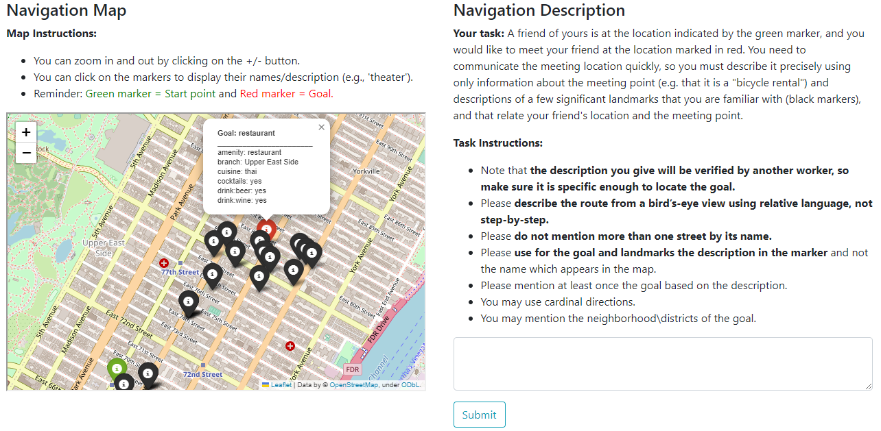
Task 1: Instruction Writing
Using the RVS map-graph (Section 2), we generated the starting points and (within 2km) the respective goal points. The instructor could view the points on an interactive map with geo-data from OSM, and displayed landmarks along the route, near the goal, in the general area and beyond the route. The goal and nearby landmarks were not shown by their proper names, e.g., instead of ‘St. Vincent de Paul Church’ the marker displayed ‘a church’. The instructor could zoom in/out and pan to view the environment. The instructor was requested to describe the location of the goal in relation to the starting point and landmarks, rather than providing a step-by-step route description. To prevent easy geolocation by current navigation and geolocation systems, such as street corners, the instructor was restricted to mentioning a maximum of one street by name.
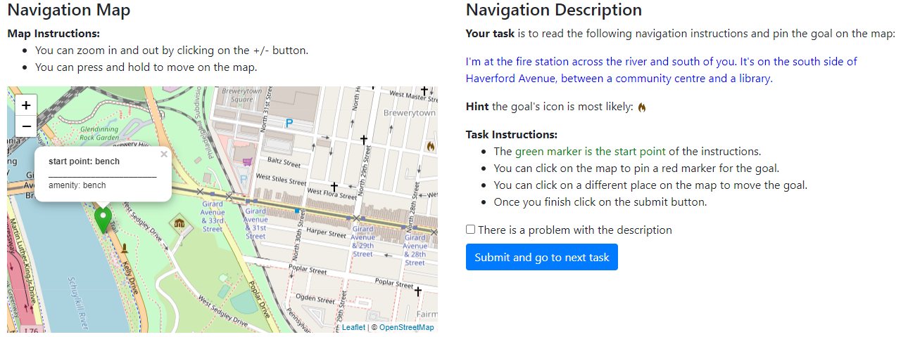
Task 2: Validation
In this task, the follower is asked to follow the instruction displayed, by pinning the goal location on an interactive map. As the map includes sign symbols of places (e.g., a cross symbol to denote a church), the display also includes a legend with the equivalent symbols. An instruction is considered qualified if the follower pins the goal within 100 meters. This threshold is the maximum radius of the geoshape of the generated goal from Task 1. Participants were also requested to flag problematic instructions, i.e., those that did not follow the rules in the instruction writing task. To determine the agreement rate among participants, 50% of the instructions were validated by at least two participants.
| City |
|
|
|
|
|
|
|
||||||||||||||
| Manhattan | 32.5 | 20,979 | 8,103 | 1,098.94 | 43.73 | 3.99 | 6,365 | ||||||||||||||
| Pittsburgh | 34.5 | 4,998 | 1,023 | 960.52 | 41.95 | 3.93 | 2,195 | ||||||||||||||
| Philadelphia | 74.5 | 10,302 | 1,278 | 1,096.66 | 42.96 | 3.95 | 2,438 |
| RVS | RUN | RxR | Touchdown | |||||||
| Phenomenon | Example from RVS | |||||||||
| Proper Names | 100 | 2 | 100 | 5.96 | 0 | 0 | 0 | 0 | …Duane Reade pharmacy… | |
| Descriptions | 96 | 2.48 | 8 | 0.12 | 100 | 8.3 | 100 | 9.2 | …There is a church across the street… | |
| Coreference | 64 | 0.88 | 40 | 0.48 | 64 | 5.3 | 60 | 1.1 | …It’s on the same block as… | |
| Count | 28 | 0.36 | 8 | 0.08 | 32 | 0.44 | 36 | 0.4 | …Southwest of the school are two bicycle parkings. | |
| Cardinal Direction | 96 | 2.2 | 16 | 0.2 | 0 | 0 | 0 | 0 | Go southwest… | |
| Complex shapes | 60 | 1.08 | 44 | 0.76 | 20 | 0.2 | 8 | 0.8 | …a block west of the square shaped park… | |
| Allocentric Relation | 88 | 1.52 | 4 | 0.04 | 76 | 2.4 | 68 | 1.2 | …It is west of the bridge… | |
| Egocentric Relation | 4 | 0.04 | 76 | 1.36 | 60 | 2.3 | 92 | 3.6 | You will pass an Ace Hardware on your left | |
| Temporal Condition | 8 | 0.08 | 72 | 1.56 | 52 | 0.8 | 84 | 1.9 | …Go straight south until you pass the library… | |
| Explicit Actions | 0 | 0 | 100 | 3.2 | 96 | 0.8 | 100 | 2.8 | …Turn left. Continue forward… | |
| State Verification | 20 | 0.2 | 56 | 0.64 | 84 | 3.1 | 72 | 1.5 | …you will see me at the alcohol shop. | |
| Negative State Verification | 4 | 0.04 | 4 | 0.04 | 0 | 0 | 0 | 0 | …If you see a bike parking, you have gone too far. | |
| Spatial Knowledge Siegel and White (1975) | Route | 4 | n/a | 84 | n/a | 100 | n/a | 100 | n/a | …turn right on the next street… |
| Survey | 96 | n/a | 16 | n/a | 0 | n/a | 0 | n/a | Head east toward the river… | |
| Feature | p-value |
|
F-test | ||
| Num. of entities4 | 0.56 | 0.56 | 0.99 | ||
| Num. of tokens | 0.0 | 0.0 | 2.92 | ||
| Human distance error | 0.0 | 0.0 | 2.43 |
Instructor Training
The main challenge of the collection process is training instructors to write high-quality instructions based on survey knowledge (rather than step-by-step agent-centered descriptions). To address this challenge, the following procedure was implemented: (1) The process starts by collecting an initial seed of ‘well-formed’ survey-based instructions written by a geospatial expert. (2) At least three ‘well-formed’ survey-based knowledge instructions were presented to an unqualified participant one after the other, and the instructor was requested to pinpoint the goal on a map. (3) Once the instruction was written by the instructor, it was reviewed by a geospatial expert who provided feedback. (4) If a participant successfully produced three well-formed survey-based instructions in a row, the instructor was considered qualified. Every instruction given by a qualified instructor was added to the bank of well-formed survey-based instructions and could be shown to other instructors in training. As more instructors became qualified, the variety of examples increased.
Quality Assessment
We ensured instruction quality by sampling instructions, discarding poor ones, and giving feedback throughout the collection process based on the following criteria: (1) participants who consistently received low distance errors in the verification task (less than 30m average), as it might indicate they gave step-by-step low-level instructions that are easier to follow; (2) instructions that received high distance errors (at least one verification over 2000m); and (3) instructions from participants who did not participate for over a month. For participants who failed their reviews (i.e., did not follow the instructions), we reviewed their next three instructions.
4 Data Statistics and Analysis
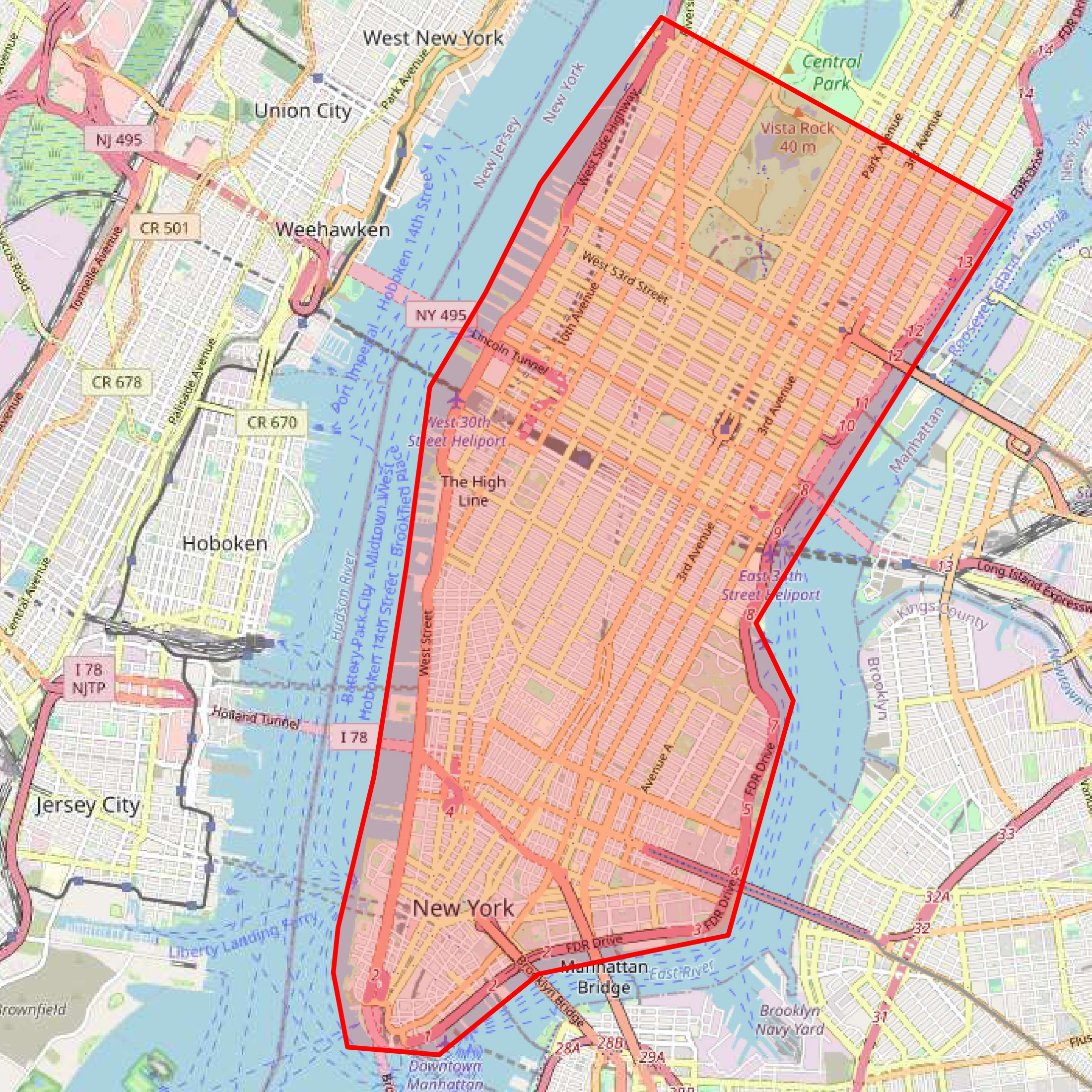
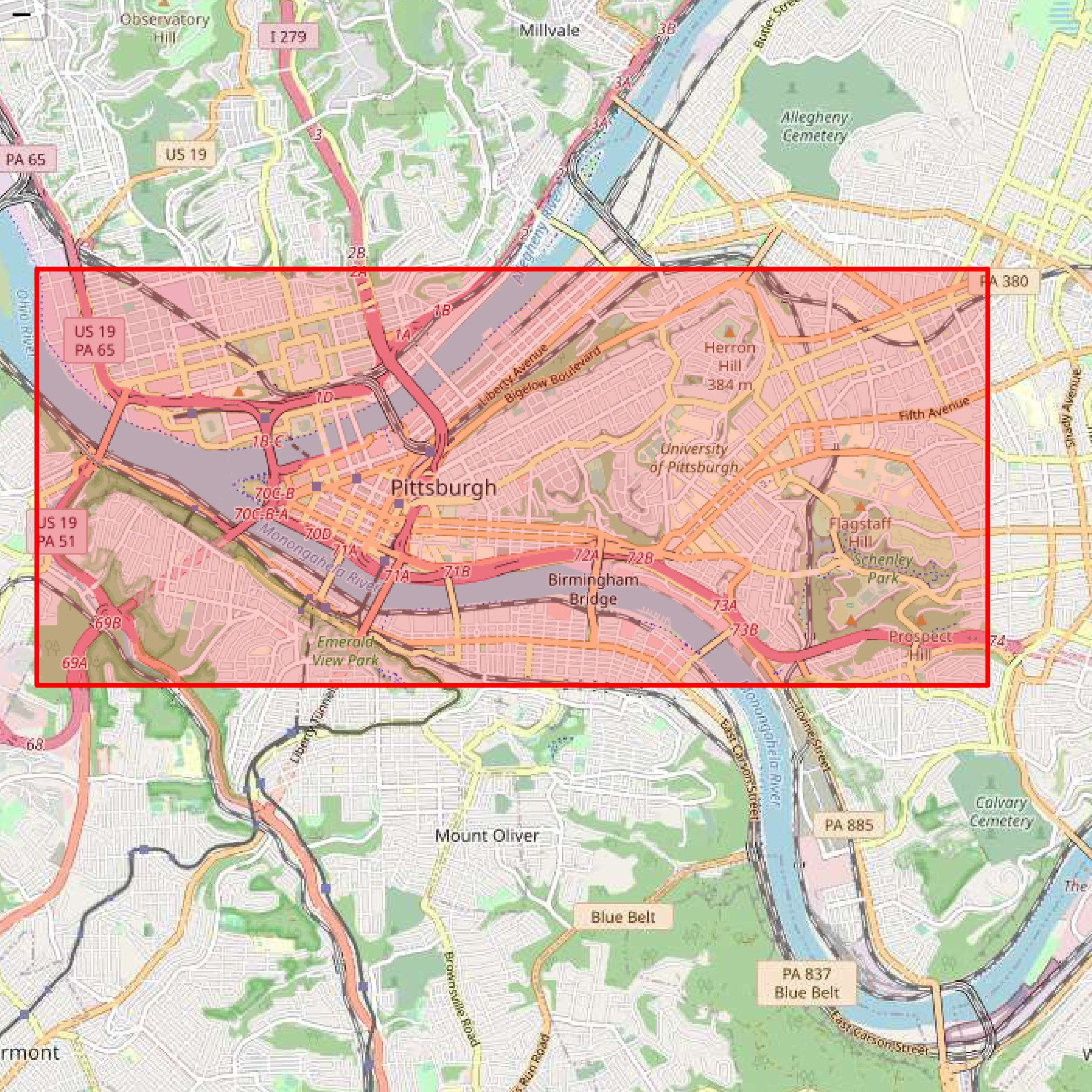
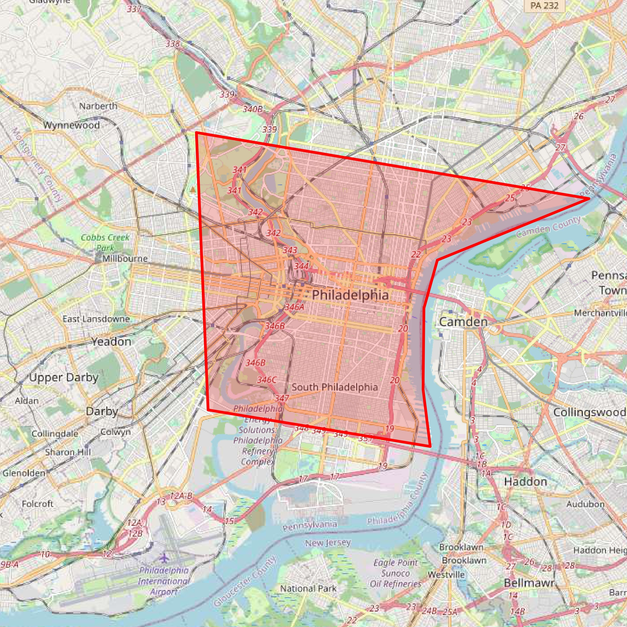
The RVS dataset contains 10,404 validated instructions paired with start and goal coordinates. The locations are divided among three cities: Manhattan, Pittsburgh, and Philadelphia (Figure 2 and Table 1). In the instruction writing task, 146 different participants provided survey-knowledge instructions. 149 participants completed the validation task, correctly validating 10,404 out of 16,104 tasks (64%). 89% of validations achieved correct location within 100 meters, indicating high human agreement.
We conducted a qualitative linguistic analysis of RVS to understand the type of geospatial reasoning required to solve the RVS task. We randomly sampled and annotated 25 examples from the Manhattan and Pittsburgh areas of RVS and compared them to previous datasets: RUN (Paz-Argaman and Tsarfaty, 2019), Touchdown (Chen et al., 2019), and RxR (Ku et al., 2020). Table 2 details this analysis. While Touchdown and RxR contain only mentions of indefinite descriptions, and RUN contains almost exclusively proper names, the RVS dataset contains a relatively balanced use of both descriptions and proper names (not near the goal). This creates a realistic challenge, reflecting the various ways people refer to landmarks.
Crucially, instructions based on survey knowledge use allocentric rather than egocentric spatial relations. Since RxR and Touchdown rely on a street/room-level view of the environment and their participants have only a short time to become familiar with the environment, the instructions contain less spatial allocentric reasoning than RVS. The RVS dataset displays more allocentric phenomena than the RUN dataset, even though both datasets include a map. This is because the RUN dataset encourages participants to use egocentric relations by displaying examples of egocentric relations. Accordingly, as shown in Table 2, geospatial measures found that RVS contains more survey-based instruction in comparison to the other datasets.
On top of that, RUN, RXR, and Touchdown all contain sequential instructions that include many explicit actions and state verifications, making it easier for the model to predict the correct action and verify it after the action is taken. In contrast, the new RVS dataset includes non-sequential instructions with relatively few state verifications and no explicit actions.
| Token | Count | Type |
| Carson | 65 | street and bridge |
| Forbes | 62 | avenue and sport stadium |
| Pittsburgh | 54 | city, station and university |
| Allegheny | 29 | avenue |
| Smallman | 23 | street |
To prevent simple string-match solutions, the goal location in RVS is always given by its type (e.g., ‘restaurant’, ‘parking’ etc.) and not by its proper name. In Table 3 we perform one-way analysis of variance (ANOVA) tests, to check if there are entity types easier to locate than others, and if the type affects the instructions. We found that the number of entities and tokens in instructions varied with goal type (p<0.05), but human distance error did not, indicating that human ability to geolocate the goal is not affected by its entity type.
Our out-of-vocabulary (OOV) analysis shows that, unlike previous navigation datasets (Chen et al., 2019; Ku et al., 2020; Anderson et al., 2018; MacMahon et al., 2006), RVS presents a challenge with novel entities in a city-split setup, training on one city and testing on a different unseen city. Specifically, our analysis of the vocabularies of two different cities --- Manhattan and Pittsburgh --- shows that 36.85% of the Pittsburgh vocabulary is OOV, i.e., the tokens do not appear in the Manhattan vocabulary. Table 4 shows the top-5 OOV tokens in Pittsburgh. 68% of OOV tokens are commonly used (82% of the OOV occurrences) city-specific named entities, like ‘Carson Street’. Thus, a city-split creates a profound OOV grounding challenge for previously unseen entities.
5 Models for RVS
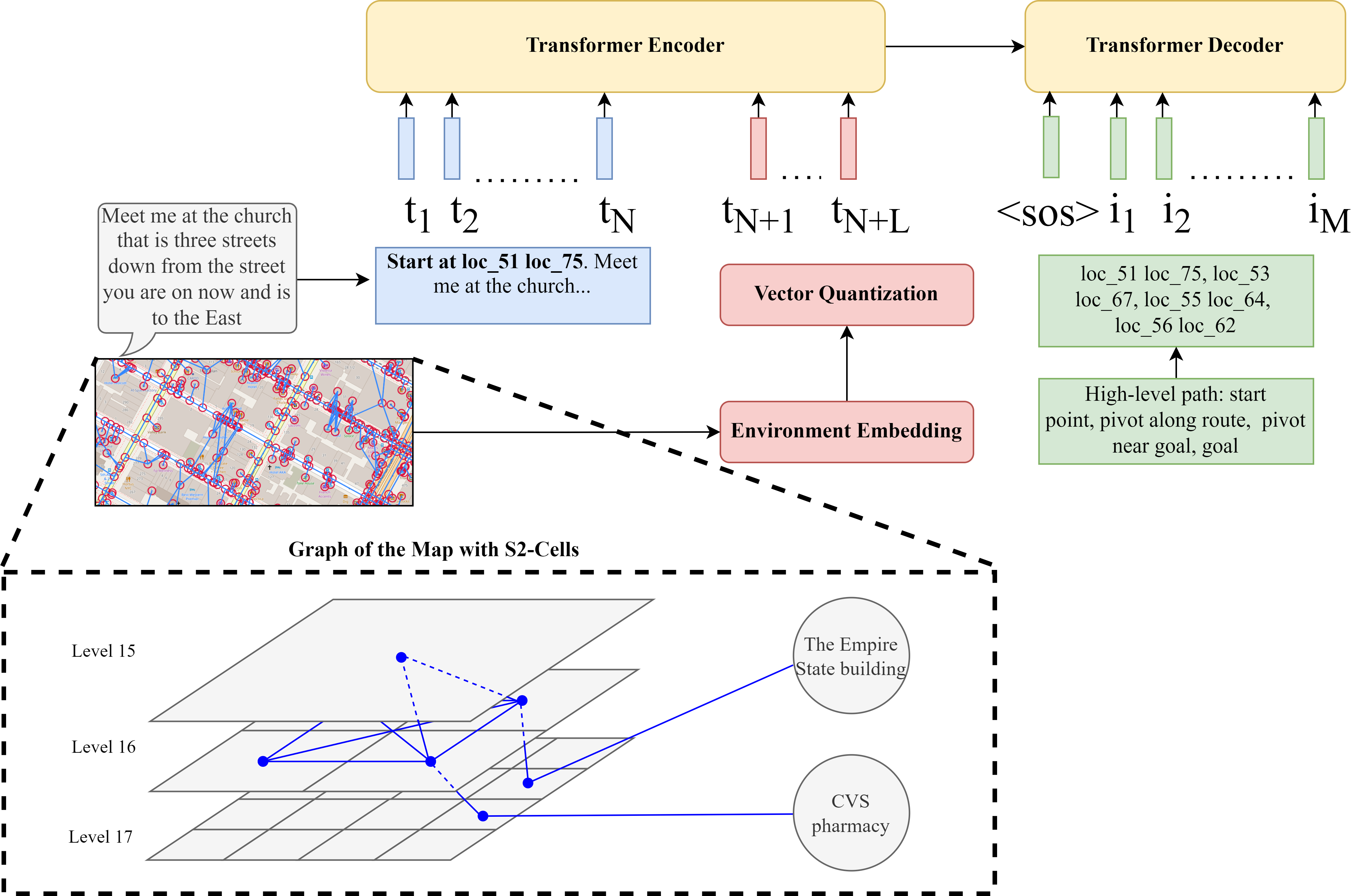
As RVS presents a new multimodal task with unique challenges, we aimed to provide a strong baseline based on our insights from Section 4. We model RVS as a sequence-to-sequence problem, where we map the sequence of tokens in the instruction to a sequence of S2-Cells.555S2Cells are based on S2-geometry, a hierarchical discretization of the Earth’s surface (Hilbert, 1935).
Encoder
The encoder encodes the instruction and the starting point’s representation. Inspired by Lu et al. (2022), who converted pixels to text-based axis locations, we transformed the map’s S2-grid into a two-dimension discrete coordinate system (‘locX, locY’). The starting point’s coordinate is assigned to the S2-Cell containing its geometry. The S2-Cell is linked to an axis position, so the starting position is also assigned an axis position.
Decoder
Since this is essentially a navigation task without a step-by-step path, we train our model to generate a high-level path, consisting of a sequence of locations starting with the starting point, followed by prominent landmarks ordered by their directional position from the goal, and ending with the goal. We extracted the prominent landmarks based on the RVS map-graph. As in the encoder, we represent the location in a ‘locX, locY’ format.
| Method | 100m Accuracy | 250m Accuracy | Mean Error | Median Error | Max Error | AUC of Error | |
| \cellcolor[HTML]EFEFEFManhattan Seen-city Development Results | |||||||
| Human | 88.12 | 95.64 | 74 | 4 | 2,996 | 0.10 | |
| Stop | 0.00 | 1.54 | 1,084 | 1,124 | 1,929 | 0.41 | |
| Center | 0.27 | 1.45 | 930 | 998 | 1,000 | 0.40 | |
| Landmark | 0.54 | 5.26 | 776 | 815 | 1,384 | 0.39 | |
| T5 | 27.92 (0.39) | 52.63 (0.45) | 362 (9) | 231 (3) | 2,957 (641) | 0.32 (0.00) | |
| T5+Graph | 29.40 (1.18) | 54.67 (1.04) | 357 (7) | 216 (8) | 3,889 (826) | 0.31 (0.01) | |
| \cellcolor[HTML]EFEFEFPittsburgh Unseen-Development Results | |||||||
| Human | 86.94 | 92.94 | 99 | 7 | 2,951 | 0.13 | |
| Stop | 0.00 | 2.05 | 960 | 954 | 1,912 | 0.40 | |
| Center | 0.00 | 0.10 | 992 | 999 | 999 | 0.41 | |
| Landmark | 1.47 | 9.48 | 677 | 691 | 1,345 | 0.38 | |
| T5 | 0.49 (1.47) | 2.34 (1.44) | 1,171 (24) | 1,107 (14) | 4,701 (101) | 0.41 (0.00) | |
| T5+Graph | 0.49 (1.01) | 2.91 (1.37) | 1,067 (77) | 1,039 (56) | 4,102 (727) | 0.40 (0.00) | |
| \cellcolor[HTML]EFEFEFPhiladelphia Unseen-city Zero-shot Results | |||||||
| Human | 93.64 | 97.97 | 27 | 3 | 2,708 | 0.05 | |
| Stop | 0.00 | 1.80 | 1,096 | 1,135 | 1,958 | 0.41 | |
| Center | 0.16 | 0.47 | 942 | 998 | 1,000 | 0.41 | |
| Landmark | 1.02 | 7.90 | 707 | 713 | 1,384 | 0.38 | |
| T5 | 0.26 (0.05) | 1.80 (0.27) |
|
1,308 (35) | 6,911 (454) | 0.42 (0.00) | |
| T5+Graph | 0.31 (0.05) | 1.93 (0.20) | 1,140 (16) | 1,161 (8) | 5,277 (372) | 0.41 (0.00) | |
| Split | Min | Max | Avg. | Example from RVS | |
| Seen-City | 61 | 3 | 9 | 5.4 | I am northeast of you at a toilet near the corner of Bayard Street. To its south is a park and the Louis J. Lefkowitz State Office Building… |
| Unseen-City | 13 | 2 | 8 | 5.05 |
| Type of Pred. and True Goal Relation | ||
| On the same S2-Cell | 25 | 5 |
| Same cardinal-direction from start point | 95 | 19 |
| On the same street | 45 | 9 |
| Have the same type of entity | 50 | 10 |
The World as a Graph
A location can be represented by its position (where the location is) or by its semantics (what is present at the location, e.g., ‘a bar’). Semantic knowledge is crucial for grounding mentioned entities to their physical references in the environment. To this end, we aim to connect the semantic and positional knowledge using a novel RVS map-graph. The RVS map-graph is a heterogeneous graph containing location nodes (semantic) and S2-cell nodes (positional). First, we connected each location node to its smallest containing S2-cell (see Figure 3), also instantiating each S2-cell as an independent node in the graph. Then, as the S2-geometry is a hierarchical structure, we add both within-level and between-level edges between S2-cell nodes. Specifically, we connect each S2-cell to its immediate neighbors at the same level, and we connect each S2-cell to its containing S2-cell at the next level up in the hierarchy (see Figure 3). To learn a joint embedding space for locations and S2-cells, we compute random walks on the graph using node2vec algorithm (Grover and Leskovec, 2016). Following Yu et al. (2021), we use linear projection to cluster the graph embeddings into K categories using the k-means algorithm with cosine similarity distance. A new token is assigned to each category and added to the tokenizer’s vocabulary. We perform multiple clusters and pass the graph’s tokens with the instruction’s tokens to the transformer encoder.
6 Experimental Setup
Evaluation
We use six evaluation metrics: (1) 100m accuracy, the task is considered completed if the agent is within a 100m distance from the goal; (2) 250m accuracy for coarse-grained accuracy evaluation; (3) mean distance error; (4) median distance error; (5) maximum distance error; and (6) area under the curve (AUC) distance error.
Setup and Data-Split
We use a zero-shot (ZS) city-based split, where we train on one city, validate on a second city, and test on a third city. Specifically, RVS’s setup consists of (i) a training-set containing 7,000 instructions from Manhattan; (ii) a seen-city development-set containing 1,103 instructions from Manhattan; (iii) an unseen-city development-set containing 1,023 instructions from Pittsburgh; and (iv) a test-set containing 1,278 instructions from Philadelphia. The ZS split raises profound challenges (e.g., OOV) at inference time, as described in Section 4.
Learning
Systems
We evaluate three non-learning baselines: (1) Stop: predicts the starting point as the goal location; (2) Center: predicts the closest location towards the center of the region within a 1000-meter radius from the starting point; (3) Landmark: predicts the location of a prominent landmark in the map within a radius of 1000 meters. A landmark is considered prominent if it has one of the following tags (appearing in descending order of importance): (a) Wikipedia page; (b) Wikidata page; (c) a part of a brand; (d) a tourist attraction; (e) an amenity; and (f) a shop.
7 Results
Table 5 shows the seen-city development, and unseen-city zero-shot (ZS) results for our six evaluation metrics. The human performance provides an upper bound for the RVS task performance, while the simple Stop is a simple lower bound baseline. Although the T5+Graph outperforms the non-learning baselines (Stop, Center, and Landmark) in the seen-city split, there is still a gap of 58.72% and 40.97% in the 100m and 250 accuracies, respectively. The Landmark model outperforms other non-learning models, suggesting that the goal location is more likely to be around prominent landmarks than in other areas.
Despite the 2km maximum distance between the start and goal, we did not constrain our models or teach them S2-Cell distances. So the maximum error of the learned models was greater than 2km. The improved performance of the T5+Graph over the T5 indicates that the added graph can capture semantic geospatial information.
The novel ZS city-split setup we introduced provides a profound challenge for natural language understanding due to the appearance of new spatial relations and new entities in the environment. This can be seen in the inability of the learning model to generalize from seen to unseen environments, resulting in low performance, even underperforming the non-learning Landmark baseline.
Tables 6 and 7 show an error analysis of 20 examples of the T5+Graph’s results in seen-city and unseen-city splits. As shown in Table 6, the model must consider multiple spatial relations to handle RVS. 666A comparative analysis of 20 RXR instructions revealed that up to two spatial relations per navigational step necessitate reasoning for successful completion. However, the model only successfully manages to predict a goal that matches the spatial relations mentioned in the text in 61% and 13% for the seen-city and unseen-city splits, respectively. Table 7 shows that in the seen-city split, the model correctly identifies the cardinal directions in most cases, suggesting that it has learned the outline configuration of the map. In half of the cases, the model correctly identifies the type of the entity. The model correctly identified the street in 45% of cases, and in 88.89% of those cases, the street was mentioned by name in the text. This is lower than the 90% of all sampled instructions that mentioned street names, suggesting that simply mentioning a street by name is not sufficient for the model to correctly produce a location on that street. In 25% of the cases, the granularity of the S2-Cells is not high enough to distinguish between the predicted and true goal, suggesting that a higher level of S2-Cell could reduce these cases.
Following Table 3, we conducted an ANOVA test and found no correlation between goal type and distance error for T5+Graph (p-value = 0.34).
8 Related Work
As people move they perceive their surroundings and acquire knowledge of the space, known as cognitive mapping (Tolman, 1948). One influential cognitive mapping theory (Siegel and White, 1975) divides cognitive mapping ability into three levels. Landmark knowledge, consisting of landmarks (e.g., mountains and buildings) and their attributes (e.g., location, size, color), Route knowledge, altered by the traveler’s changing viewpoint (Taylor and Tversky, 1992a, b, 1996) and coded directly (e.g., “turn right, then straight”) (Tlauka and Wilson, 1994), or as condition-action rules based on landmark-direction associations (e.g., “turn right at the church, then straight” (Kuipers, 1978; Thorndyke, 1981)), and survey knowledge, where people form a ‘cognitive map’ of the environment, an overview of the geospatial layout, and gain awareness of relationships between different geospatial components, even outside the route. Survey knowledge is independent of a person’s own position, and enables her to form different routes, refer to cardinal directions, describe landmarks at different resolution levels, and describe complex shapes of abstract features such as ‘blocks’. Such information is less likely to be acquired from direct experience in the environment, but is portrayed on maps (Thorndyke and Hayes-Roth, 1982). Thus, instructions based on such knowledge mirror the complex understanding of the environment.
In grounded NLP tasks, participants acquire knowledge over an environment provided with the task. This environment can be based on different sources, most commonly visual sensors with real (Qi et al., 2020; Blukis et al., 2018; Wang et al., 2018) or synthetic imagery (Yan et al., 2018; Misra et al., 2018; Shridhar et al., 2020). In a visual environment, participants travel through the environment, view it from a point on the ground that is on the same plane as the objects, and acquire route knowledge. Thorndyke and Hayes-Roth (1982) found that subjects who learned an environment by walking through it were limited to route-based knowledge and used egocentric spatial relation expressions (e.g., ‘on your right’) in their instructions. This observation was reinforced by Chen et al. (2019) analysis of Touchdown (Chen et al., 2019) and R2R Anderson et al. (2018) — two navigation tasks with walk-through environments.
Another type of environment uses maps (Anderson et al., 1991; Paz-Argaman and Tsarfaty, 2019; Vogel and Jurafsky, 2010; Levit and Roy, 2007; Vasudevan et al., 2021; de Vries et al., 2018), where instructors can view the environment from above and gain survey knowledge of global geospatial relations. However, previous works with maps have either presented small, simplistic environments (Anderson et al., 1991; de Vries et al., 2018) or the task’s setup has encouraged participants to give egocentric sequential instructions limited to the route (Paz-Argaman and Tsarfaty, 2019; de Vries et al., 2018; Vasudevan et al., 2021). In contrast, RVS focuses on instructions that encode survey knowledge and require configurational and allocentric reasoning over a large, entity-dense environment.
There are sharp differences between indoor (Ku et al., 2020; Anderson et al., 2018) and outdoor (Chen et al., 2019; Paz-Argaman and Tsarfaty, 2019; de Vries et al., 2018; Vasudevan et al., 2021; Anderson et al., 1991) navigation instructions. Indoor environments contain many entities referred to as definite descriptions (e.g., ‘the chair’) and few landmarks that can be referred to by their proper name (‘The Blue Room in the White House’). In outdoor environments, people tend to mix the use of proper names (e.g., ‘the Empire State building’) and definite descriptions (e.g., ‘the school’). However, previous outdoor navigation tasks either contain only definite descriptions (Chen et al., 2019; Vasudevan et al., 2021) or almost exclusively proper names (Paz-Argaman and Tsarfaty, 2019). RVS contains a balanced amount of both.
9 Where Do We Go From Here?
Bridging the Human-AI Performance Gap
A substantial gulf separates current models’ performance from human performance in the RVS task. In seen environments, models lag behind by 58.72% in 100-meter accuracy and 212 meters in median error. This gap widens further in unseen environments, with a staggering 93.33% difference in 100-meter accuracy and 1,158 meters in median error. The challenge of bridging this gap could unlock thrilling research avenues that push the boundaries of this task.
Spatial Large Language Models
One promising approach to tackle this challenge lies in the development of spatial large language models (LLMs) specifically pre-trained for geolocation based on textual descriptions. Such models could unlock the vast potential of textual geospatial information readily available online (Spink et al., 2002; Sanderson and Kohler, 2004). They could empower natural language-driven geospatial queries and support Geo-Information Retrieval (GIR) processes. Additionally, generating instructions that describe a location based on relative landmarks – rather than explicit actions like ‘turn right’, which are not always relevant or sufficient for navigation in many parts of the world --- can enable people to follow instructions which are less ‘robotic’, more natural, and more relevant. Looking beyond navigation, spatial LLMs could also play a crucial role in enhancing the accessibility and usability of geospatial data. By enabling users to interact with maps and spatial information using natural language, LLMs can bridge the gap between human language and spatial data representations, making these resources more accessible to a wider range of users.
Seeing the Streets: Integrating Visual Cues
Humans perceive the world through different signals (e.g., images and sounds) that they get from their senses. Similarly, to understand the world, artificial intelligence research also tries to solve problems that use multimodal data (Antol et al., 2015; Paz-Argaman et al., 2020; Ji et al., 2022). While maps are one modality that can be used in navigation, it is interesting to note that regions of the maps can be augmented by street view images, such as Google Street View imagery,777StreetLearn dataset Mirowski et al. (2019) contains images for the Manhattan and Pittsburgh regions in RVS. to integrate the visual modality in the RVS dataset. Alternatively, the RVS dataset represents maps as symbolic world representations, which do not account for the visual perception of maps by humans. Therefore, it would be interesting to use image representation instead of graphs in the RVS dataset.888The GitHub repository for the RVS dataset contains maps’ imagery, which can be accessed at the following link: https://github.com/OnlpLab/RVS Visual descriptions that appear in RVS, like the shape of a "triangular block" are far more evident in images than in the symbolic map representation.
10 Conclusion
This work presents the RVS task and dataset, which present a new focus on understanding geospatial instructions based on survey knowledge of urban environments. Our analysis shows that the data presents profound spatial-reasoning challenges such as allocentric relations, multiple relations, cardinal directions, and more, requiring models with novel representations of the environment that can enhance and complement the language understanding capacity of LLMs. Our results show that our zero-shot city split set-up presents a major challenge, leaving ample space for further research on this benchmark and task.
Limitations
In the data collection process (described in Section 3) we showed participants an interactive map with the start and goal points, as well as landmarks along the route, near the goal, and in the general area beyond the route. One of our guidelines for collecting the data is to allow participants to use a mix of proper names and definite descriptions without giving the location of the goal by mentioning proper names adjacent to it, so that a named entity recognition (NER) system would not be able to locate the goal. To enforce this guideline, we displayed the landmarks with different levels of information: for landmarks near the goal (less than 200m), we displayed partial information, excluding the proper name; for landmarks far from the goal (more than 200m), we displayed all the information. For example, for a landmark of a restaurant with the tag name ‘Kofoo’, we displayed multiple tags without the tag name if it was located near the goal: ‘amenity: restaurant, cuisine: ‘korean’. This allowed the participant to refer to ‘Kofoo’ as a ‘restaurant‘ or a ‘korean restaurant’. To achieve this, we displayed pop-up markers of the landmarks and requested the participants to provide the instructions using only descriptions of landmarks in the pop-up markers (see Appendix D). While aiming to minimize information overload (IO), our study presented only 40 of these landmark pop-up markers on the map. Landmark selection prioritized prominence based on pre-defined tags like "wikipedia" and "brand." However, this approach restricted user choice and potentially introduced bias. In dense areas like Manhattan, showcasing merely 40 landmarks concealed 99.81% of potential reference landmarks. Moreover, relying solely on specific tags may have neglected other prominent features readily used for navigation, such as easily identifiable landmarks on street corners. This potential mismatch between presented and naturally chosen landmarks could have influenced navigational accuracy. While increasing the displayed landmarks seems intuitive, it could exacerbate IO and prolong search times for relevant landmarks. Thus, the challenge lies in striking a balance between minimizing IO and providing sufficient landmarks for accurate wayfinding.
Acknowledgements
This research has been funded by the European Research Council (ERC), grant number 677352 and by a grant from the Israeli Science Foundation (ISF) number 670/23, for which we are grateful. The research was further supported by a KAMIN grant from the Israeli Innovation Author- ity, and computing resources kindly funded by a VATAT grant and via the Data Science Institute from Bar-Ilan University (BIU-DSI). We are also grateful for the additional support provided by a Google grant.
References
- Abebrese (2019) Kwasi Abebrese. 2019. Implementing street addressing system in an evolving urban center. A case study of the Kumasi metropolitan area in Ghana. Ph.D. thesis, Iowa State University.
- Anderson et al. (1991) Anne H Anderson, Miles Bader, Ellen Gurman Bard, Elizabeth Boyle, Gwyneth Doherty, Simon Garrod, Stephen Isard, Jacqueline Kowtko, Jan McAllister, Jim Miller, et al. 1991. The hcrc map task corpus. Language and speech, 34(4):351--366.
- Anderson et al. (2018) Peter Anderson, Qi Wu, Damien Teney, Jake Bruce, Mark Johnson, Niko Sünderhauf, Ian Reid, Stephen Gould, and Anton Van Den Hengel. 2018. Vision-and-language navigation: Interpreting visually-grounded navigation instructions in real environments. In Proceedings of the IEEE conference on computer vision and pattern recognition, pages 3674--3683.
- Antol et al. (2015) Stanislaw Antol, Aishwarya Agrawal, Jiasen Lu, Margaret Mitchell, Dhruv Batra, C Lawrence Zitnick, and Devi Parikh. 2015. Vqa: Visual question answering. In Proceedings of the IEEE international conference on computer vision, pages 2425--2433.
- Blukis et al. (2018) Valts Blukis, Nataly Brukhim, Andrew Bennett, Ross A Knepper, and Yoav Artzi. 2018. Following high-level navigation instructions on a simulated quadcopter with imitation learning. arXiv preprint arXiv:1806.00047.
- Chen et al. (2019) Howard Chen, Alane Suhr, Dipendra Misra, Noah Snavely, and Yoav Artzi. 2019. Touchdown: Natural language navigation and spatial reasoning in visual street environments. In Proceedings of the IEEE/CVF Conference on Computer Vision and Pattern Recognition (CVPR).
- de Vries et al. (2018) Harm de Vries, Kurt Shuster, Dhruv Batra, Devi Parikh, Jason Weston, and Douwe Kiela. 2018. Talk the walk: Navigating new york city through grounded dialogue. arXiv preprint arXiv:1807.03367.
- Grover and Leskovec (2016) Aditya Grover and Jure Leskovec. 2016. node2vec: Scalable feature learning for networks. In Proceedings of the 22nd ACM SIGKDD international conference on Knowledge discovery and data mining, pages 855--864.
- Hayward and Tarr (1995) William G Hayward and Michael J Tarr. 1995. Spatial language and spatial representation. Cognition, 55(1):39--84.
- Hilbert (1935) David Hilbert. 1935. Über die stetige abbildung einer linie auf ein flächenstück. In Dritter Band: Analysis· Grundlagen der Mathematik· Physik Verschiedenes, pages 1--2. Springer.
- Hu et al. (2023) Yingjie Hu, Gengchen Mai, Chris Cundy, Kristy Choi, Ni Lao, Wei Liu, Gaurish Lakhanpal, Ryan Zhenqi Zhou, and Kenneth Joseph. 2023. Geo-knowledge-guided gpt models improve the extraction of location descriptions from disaster-related social media messages. International Journal of Geographical Information Science, pages 1--30.
- Jayannavar et al. (2020) Prashant Jayannavar, Anjali Narayan-Chen, and Julia Hockenmaier. 2020. Learning to execute instructions in a minecraft dialogue. In Proceedings of the 58th annual meeting of the association for computational linguistics, pages 2589--2602.
- Ji et al. (2022) Anya Ji, Noriyuki Kojima, Noah Rush, Alane Suhr, Wai Keen Vong, Robert D Hawkins, and Yoav Artzi. 2022. Abstract visual reasoning with tangram shapes. arXiv preprint arXiv:2211.16492.
- Krause and Cohen (2020) Amir Krause and Sara Cohen. 2020. Deriving geolocations in wikipedia. In Proceedings of the 29th ACM International Conference on Information & Knowledge Management, pages 3293--3296.
- Krause and Cohen (2023) Amir Krause and Sara Cohen. 2023. Geographic information retrieval using wikipedia articles. In Proceedings of the ACM Web Conference 2023, pages 3331--3341.
- Ku et al. (2020) Alexander Ku, Peter Anderson, Roma Patel, Eugene Ie, and Jason Baldridge. 2020. Room-Across-Room: Multilingual vision-and-language navigation with dense spatiotemporal grounding. In Conference on Empirical Methods for Natural Language Processing (EMNLP).
- Kuipers (1978) Benjamin Kuipers. 1978. Modeling spatial knowledge. Cognitive science, 2(2):129--153.
- Lachmy et al. (2022) Royi Lachmy, Valentina Pyatkin, Avshalom Manevich, and Reut Tsarfaty. 2022. Draw me a flower: Processing and grounding abstraction in natural language. Transactions of the Association for Computational Linguistics, 10:1341--1356.
- Levit and Roy (2007) Michael Levit and Deb Roy. 2007. Interpretation of spatial language in a map navigation task. IEEE Transactions on Systems, Man, and Cybernetics, Part B (Cybernetics), 37(3):667--679.
- Loshchilov and Hutter (2017) Ilya Loshchilov and Frank Hutter. 2017. Fixing weight decay regularization in adam. CoRR, abs/1711.05101.
- Lu et al. (2022) Jiasen Lu, Christopher Clark, Rowan Zellers, Roozbeh Mottaghi, and Aniruddha Kembhavi. 2022. Unified-io: A unified model for vision, language, and multi-modal tasks. arXiv preprint arXiv:2206.08916.
- MacMahon et al. (2006) Matt MacMahon, Brian Stankiewicz, and Benjamin Kuipers. 2006. Walk the talk: Connecting language, knowledge, and action in route instructions. Def, 2(6):4.
- Mirowski et al. (2019) Piotr Mirowski, Andras Banki-Horvath, Keith Anderson, Denis Teplyashin, Karl Moritz Hermann, Mateusz Malinowski, Matthew Koichi Grimes, Karen Simonyan, Koray Kavukcuoglu, Andrew Zisserman, et al. 2019. The streetlearn environment and dataset. arXiv preprint arXiv:1903.01292.
- Misra et al. (2018) Dipendra Misra, Andrew Bennett, Valts Blukis, Eyvind Niklasson, Max Shatkhin, and Yoav Artzi. 2018. Mapping instructions to actions in 3d environments with visual goal prediction. arXiv preprint arXiv:1809.00786.
- Paz-Argaman et al. (2020) Tzuf Paz-Argaman, Yuval Atzmon, Gal Chechik, and Reut Tsarfaty. 2020. Zest: Zero-shot learning from text descriptions using textual similarity and visual summarization. arXiv preprint arXiv:2010.03276.
- Paz-Argaman et al. (2023) Tzuf Paz-Argaman, Tal Bauman, Itai Mondshine, Itzhak Omer, Sagi Dalyot, and Reut Tsarfaty. 2023. Hegel: A novel dataset for geo-location from hebrew text. arXiv preprint arXiv:2307.00509.
- Paz-Argaman and Tsarfaty (2019) Tzuf Paz-Argaman and Reut Tsarfaty. 2019. RUN through the streets: A new dataset and baseline models for realistic urban navigation. In Proceedings of the 2019 Conference on Empirical Methods in Natural Language Processing and the 9th International Joint Conference on Natural Language Processing (EMNLP-IJCNLP), pages 6449--6455, Hong Kong, China. Association for Computational Linguistics.
- Plumert et al. (2007) Jodie M Plumert, John P Spencer, John P Spencer, et al. 2007. The emerging spatial mind. Oxford University Press.
- Qi et al. (2020) Yuankai Qi, Qi Wu, Peter Anderson, Xin Wang, William Yang Wang, Chunhua Shen, and Anton van den Hengel. 2020. Reverie: Remote embodied visual referring expression in real indoor environments. In Proceedings of the IEEE/CVF Conference on Computer Vision and Pattern Recognition (CVPR).
- Raffel et al. (2020) Colin Raffel, Noam Shazeer, Adam Roberts, Katherine Lee, Sharan Narang, Michael Matena, Yanqi Zhou, Wei Li, Peter J Liu, et al. 2020. Exploring the limits of transfer learning with a unified text-to-text transformer. J. Mach. Learn. Res., 21(140):1--67.
- Sanderson and Kohler (2004) Mark Sanderson and Janet Kohler. 2004. Analyzing geographic queries. In SIGIR workshop on geographic information retrieval, volume 2, pages 8--10.
- Shridhar et al. (2020) Mohit Shridhar, Jesse Thomason, Daniel Gordon, Yonatan Bisk, Winson Han, Roozbeh Mottaghi, Luke Zettlemoyer, and Dieter Fox. 2020. Alfred: A benchmark for interpreting grounded instructions for everyday tasks. In Proceedings of the IEEE/CVF Conference on Computer Vision and Pattern Recognition, pages 10740--10749.
- Siegel and White (1975) Alexander W Siegel and Sheldon H White. 1975. The development of spatial representations of large-scale environments. Advances in child development and behavior, 10:9--55.
- Spink et al. (2002) Amanda Spink, Bernard J Jansen, Dietmar Wolfram, and Tefko Saracevic. 2002. From e-sex to e-commerce: Web search changes. Computer, 35(3):107--109.
- Taylor and Tversky (1992a) Holly A Taylor and Barbara Tversky. 1992a. Descriptions and depictions of environments. Memory & cognition, 20(5):483--496.
- Taylor and Tversky (1992b) Holly A Taylor and Barbara Tversky. 1992b. Spatial mental models derived from survey and route descriptions. Journal of Memory and language, 31(2):261--292.
- Taylor and Tversky (1996) Holly A Taylor and Barbara Tversky. 1996. Perspective in spatial descriptions. Journal of memory and language, 35(3):371--391.
- Thorndyke (1981) P Thorndyke. 1981. Spatial cognition and reasoning. Cognition Social Behavior, and The Environment, 7.
- Thorndyke and Hayes-Roth (1982) Perry W Thorndyke and Barbara Hayes-Roth. 1982. Differences in spatial knowledge acquired from maps and navigation. Cognitive psychology, 14(4):560--589.
- Tlauka and Wilson (1994) Michael Tlauka and Paul N Wilson. 1994. The effect of landmarks on route-learning in a computer-simulated environment. Journal of Environmental Psychology, 14(4):305--313.
- Tolman (1948) Edward C Tolman. 1948. Cognitive maps in rats and men. Psychological review, 55(4):189.
- Tversky (1996) Barbara Tversky. 1996. Spatial perspective in descriptions. Language and space, 3:463--491.
- Tversky (2005) Barbara Tversky. 2005. Functional significance of visuospatial representations. Handbook of higher-level visuospatial thinking, pages 1--34.
- UPU (2012) UPU. 2012. Addressing the world – An address for everyone.
- Uttal (2000) David H Uttal. 2000. Seeing the big picture: Map use and the development of spatial cognition. Developmental Science, 3(3):247--264.
- Vasudevan et al. (2021) Arun Balajee Vasudevan, Dengxin Dai, and Luc Van Gool. 2021. Talk2nav: Long-range vision-and-language navigation with dual attention and spatial memory. International Journal of Computer Vision, 129:246--266.
- Vogel and Jurafsky (2010) Adam Vogel and Dan Jurafsky. 2010. Learning to follow navigational directions. In Proceedings of the 48th Annual Meeting of the Association for Computational Linguistics, pages 806--814. Association for Computational Linguistics.
- Wang et al. (2018) Xin Wang, Wenhan Xiong, Hongmin Wang, and William Yang Wang. 2018. Look before you leap: Bridging model-free and model-based reinforcement learning for planned-ahead vision-and-language navigation. arXiv preprint arXiv:1803.07729.
- Wing and Baldridge (2014) Benjamin Wing and Jason Baldridge. 2014. Hierarchical discriminative classification for text-based geolocation. In Proceedings of the 2014 conference on empirical methods in natural language processing (EMNLP), pages 336--348.
- Yan et al. (2018) Claudia Yan, Dipendra Misra, Andrew Bennnett, Aaron Walsman, Yonatan Bisk, and Yoav Artzi. 2018. Chalet: Cornell house agent learning environment. arXiv preprint arXiv:1801.07357.
- Yu et al. (2021) Jiahui Yu, Xin Li, Jing Yu Koh, Han Zhang, Ruoming Pang, James Qin, Alexander Ku, Yuanzhong Xu, Jason Baldridge, and Yonghui Wu. 2021. Vector-quantized image modeling with improved vqgan. arXiv preprint arXiv:2110.04627.
- Zhang and Choi (2021) Michael JQ Zhang and Eunsol Choi. 2021. Situatedqa: Incorporating extra-linguistic contexts into qa. arXiv preprint arXiv:2109.06157.
Appendix A Data Collection Details
Participants
We collected the RVS dataset using Amazon Mechanical Turk (MTurk). We did not collect any information that could be used to identify the participants. We presented the task to the participants as part of a research on navigation instructions. We worked with both past MTurk workers and new workers who had a 99% percentage assignment approval rate and at least 500 approved HITs. Only English speakers were allowed to participate. The base pay was $ for writing instructions and $ for completing a validation task. Instead of giving bonuses based on successful validation, we rewarded workers who generated high-quality instructions based on survey-knowledge that met our criteria, such as not mentioning more than one street by name. After evaluating worker performance through random sampling of instructions, we offered bonuses ranging from $ to $ to those who performed well. All but three of the 149 participants who took part in the validation task also participated in the instruction writing task.
Instructions vs. Descriptions
Although our ‘instructions’ are non-sequential and thus differ from typical instructions in previous navigation tasks Paz-Argaman and Tsarfaty (2019); Chen et al. (2019); Ku et al. (2020), we chose the term ‘instruction’ and not ‘description’ for the following reasons: (1) The term ‘descriptions’ is used in geolocation tasks where place descriptions are given (Paz-Argaman et al., 2023). Unlike RVS, in geolocation tasks there is no assumption for a starting point (Krause and Cohen, 2020, 2023). In RVS, we give instructions on how to find point B, given point A as a starting point. (2) Instructions are usually sequential, but they don’t have to be (e.g., a set of assembly instructions for a toy is non-sequential because the steps can be followed in any order and still result in a completed toy).
Multiple Validations
In order to determine the agreement rate among participants, at least two participants validated 50% of the instructions, as shown in Figure A.
Selection of Cities
The study selected three cities to create a realistic scenario where training is done on one city and testing is done on another. Manhattan was selected as the training set because it is the most entity-dense environment and will allow for maximum unique paths. Additionally, Manhattan and Pittsburgh were chosen because the StreetLearn dataset Mirowski et al. (2019) released Google Street View imagery for these areas, which might allow future integration of images.
![[Uncaptioned image]](/html/2402.16364/assets/img/verification_example.png)
Example of Multiple Validations: (i) starting point (green marker), (ii) goal (red marker), and (iii) predicted goal by participants (black markers).
| Model | 100m Accuracy | 250m Accuracy | Mean Error | Median Error | Max Error | AUC of Error |
| \cellcolor[HTML]EFEFEFTrain on Pittsburgh | ||||||
| T5 | 0.00 | 1.09 | 1,085 | 1,119 | 1,969 | 0.41 |
| T5+Graph | 0.18 | 2.45 | 1,219 | 1,172 | 5,954 | 0.41 |
| \cellcolor[HTML]EFEFEFTrain on Philadelphia | ||||||
| T5 | 0.00 | 1.54 | 1,085 | 1,124 | 1,929 | 0.41 |
| T5+Graph | 0.27 | 1.72 | 1,869 | 1,232 | 7,436 | 0.42 |
Path Length Limitation
To ensure accurate, precise, and geolocatable navigation instructions for participants, we implemented a two-kilometer radius limitation. Our preliminary experiments with MTurk participants revealed that they experienced difficulties in finding the goal location when the distance between the start point and the goal exceeded two kilometers. Additionally, the RVS dataset is designed to facilitate high-granularity urban geolocation, making it essential to restrict the navigation range to a manageable distance.
Appendix B T5-based models
The Graph Embedding
The graph was constructed using three levels of S2-Cells: 15, 16, and 17. At level 16, each sub-graph consisting of four neighboring S2-Cells was fully connected. All S2-Cells in the graph were linked to their parent S2-Cell based on the S2-geometry’s hierarchy (i.e., level 17 S2-Cells were connected to level 16 S2-Cells and level 16 S2-Cells were connected to level 15 S2-Cells). Extracted entities from OSM and Wikidata88footnotetext: Wikidata is a free and open knowledge base that acts as central storage for structured data of its Wikimedia sister projects, including Wikipedia, Wikivoyage, Wiktionary, Wikisource, and others were linked to the smallest level 17 S2-Cell that encompassed their geometry. The node of the entity included additional data such as its geometry, type, and name. Random walks on the graph were performed using node2vec (Grover and Leskovec, 2016).
Experimental Setup Details
For both T5-base models, we use a pre-trained ‘T5-Base’ model from Hugging Face Hub, which is licensed under the Apache License 2.0. The T5 model was trained on the Colossal Clean Crawled Corpus (C4, Raffel et al. (2020)). The cross-entropy loss function was optimized with AdamW optimizer (Loshchilov and Hutter, 2017). The hyperparameter tuning is based on the average results run with three different seeds. We used a learning rate of 1e-4. The S2-cell level was searched in [15, 16, 17, 18] and 16 was chosen. The number of clusters for the quantization process was searched in [50, 100, 150, 200, 250] and 150 was chosen. We used 2 quantization layers. Number of epochs for early stopping was based on their average learning curve. We used the following parameters for the node2vec algorithm: an embedding size of 1024, a walk length of 20, 200 walks, a context window size of 10, a word batch of 4, and 5 epochs.
B.1 S2-Geometry
S2Cells are a hierarchical discretization of the Earth’s surface, enabling efficient representation and computation of geospatial data. S2Cells are based on S2-geometry a mathematical framework for representing and computing shapes on the sphere Hilbert (1935). Each cell is a quadrilateral bounded by four geodesics (shortest path between two points on a curved surface). The top level of the hierarchy is obtained by projecting the six faces of a cube onto the unit sphere, and lower levels are obtained by subdividing each cell into four children recursively. S2Cells are globally uniform, i.e., all of the cells at the same level have the same size and shape, regardless of where they are located on the Earth’s surface. The level is defined as the number of times the cell has been subdivided (starting with a face cell). Cells levels range from 0 to 30. The smallest cells at level 30 are called leaf cells; there are of them in total, each about 1cm across on the Earth’s surface.
Appendix C Results over Alternative Splits
In Table 5 we showed the results on a split that was trained on Manhattan, with Pittsburgh as the development set and Philadelphia as the test set. However, Manhattan is demographically different from Pittsburgh and Philadelphia and contains more entities on the map. In Table 8 we show results over different permutations of the cities -- testing on Manhattan and training on either Pittsburgh or Philadelphia. However, as the development Pittsburgh set and test Philadelphia sets contain few instructions (1,103 and 1,278 instructions, respectively), it seems they do not contain enough data to support learning. This claim is supported in Table 8 which shows the results for testing on Manhattan with different training sets. The T5 model, in both splits learns to predict close locations to the starting point, or even the exact location as the starting point. It therefore does not go over the limited range of 2K distance and has very low accuracy. The T5+Graph model has a higher accuracy but the model also predicts location over the limited range, resulting in a very high mean error distance. Additionally, the results for all models trained on Pittsburgh were slightly better than the ones trained on Philadelphia, which might be due to the size of the region, Philadelphia being more than twice as large as Pittsburgh, the T5+Graph model struggles to learn connections --- i.e., grounding. --- between text and the environment.