Estimation of complex carryover effects in crossover designs with repeated measures

Abstract

It has been argued that the models used to analyze data from crossover designs are not appropriate when simple carryover effects are assumed. In this paper, the estimability conditions of the carryover effects are found, and a theoretical result that supports them, additionally, two simulation examples are developed in a non-linear dose-response for a repeated measures crossover trial in two designs: the traditional AB/BA design and a Williams square. Both show that a semiparametric model can detect complex carryover effects and that this estimation improves the precision of treatment effect estimators. We concluded that when there are at least five replicates in each observation period per individual, semiparametric statistical models provide a good estimator of the treatment effect and reduce bias with respect to models that assume either, the absence of carryover or simplex carryover effects. In addition, an application of the methodology is shown and the richness in analysis that is gained by being able to estimate complex carryover effects is evident.

1 Introduction

Crossover experimental designs are a very useful tool to analyze the effects of treatments applied to a set of experimental units (Hinkelmann and Kempthorne, 2005). In this type of study, an experimental unit receives several treatments, each one in a different period, this leads to an assembly where a sequence of treatments is applied to each unit (Cruz et al. (2023a), Cruz et al. (2023b)).

Due to the structure of crossover designs, carryover effects are part of them. Vegas et al. (2016a) defined carryover as the persistence of the effect of one treatment over treatments applied later. That is, if a treatment is applied in a certain period, then there is the possibility of a residual or carryover effect that persists in the following periods when other treatments are applied. When the carryover effect of a treatment affects the one applied in the following period, it is known as a first-order carryover effect; if it affects the one applied two periods ahead, it is known as a second-order carryover effect, and so on.
In the modeling of carryover effects, these are divided into two types: i) simple carryover, where the residual effect of one treatment equally affects each of the treatments that follow it, and ii) complex carryover, where the residual effect of the treatment affects each of the other treatments differently, that is, an interaction between treatments.

(Fleiss, 1989) and (Senn, 1992) showed that if there is complex carryover, there is greater bias in the estimation of treatment effects when simple carryover effects are assumed for the estimation model than when no carryover effects are assumed. It is also argued that the presence of simple carryover effects is an unrealistic scenario in pharmacological studies, but if it occurs, the model under the assumption of simple carryover effects does estimate better than the model without assuming the carryover effect. The problem is that the examples in (Fleiss, 1989) and (Senn, 1992) were planned with the assumption that each experimental unit is only observed once in each period, so it is impossible to estimate complex carryover effects due to the lack of degrees of freedom. Additionally, when reviewing recent studies that work with crossover designs, simple carryover effects are always assumed, or their presence is not assumed. However, it is never discussed what would happen if complex carryover effects are supposed, even when some designs present several observations of each experimental unit per period (Basu and Santra (2010), Josephy et al. (2015), Hao et al. (2015), Lui (2015), Rosenkranz (2015), Grayling et al. (2018), Madeyski and Kitchenham (2018), Kitchenham et al. (2018), Oh et al. (2003), Curtin (2017), Li et al. (2018), Jankar et al. (2020) and Cruz et al. (2023b))

The above represented an unaddressed challenge in the estimation of carryover effects, until Cruz et al. (2023a) found a methodology based on semiparametric GEE (Generalized estimating equations) that allows estimating complex carryover effects when there are several measurements of the same experimental unit within each period. This study also illustrated a simulation in a Williams design. However, other types of designs were not explored, nor were ideas given regarding estimability or the behavior of the methodology in AB/BA designs, which are very common in clinical research.

The analyses found in the scientific literature are based on the assumption of simple carryover effects, such as in Pitchforth et al. (2020), where a Williams arrangement experiment is described. In the work environment experiment, there were a total of $n=288$ participants. These participants were divided into four groups: $G1$, $G2$, $G3$, and $G4$ and each group had the same number of (72) individual participants. The periods were named Period 1, Period 2, Period 3, and Period 4, where each Period lasted 2 weeks. The four treatments involved in this experiment are office layouts labeled A: Menu (activity-based), B: Control (open plan), C: Nest (team offices), and D: Campus (zoned open plan). The structure of the crossover design is given in Table 1.

Sequence	Period 1	Period 2	Period 3	Period 4
Group 1	B	A	D	C
Group 2	C	D	A	B
Group 3	D	B	C	A
Group 4	A	C	B	D

Table 1: Structure of the crossover design in work environment experiment

In this experiment, sensors were used to detect desk occupancy. These sensors contained infrared cameras and had the functionality of establishing a region of interest within the video frame. They recorded the number of people seen within the area of interest once every 5 minutes Pitchforth et al. (2020). This variable generated a repeated measurement within each period of the binomial type during working hours (from 09:00 to 18:00), for which there were 96 measurements of the number of times that the job was occupied and those that were not occupied. This variable was analyzed using simple carryover effects in the works of (Jankar and Mandal, 2021) and Cruz et al. (2023b). Therefore, in this paper, we explore the estimability properties of complex carryover effects in crossed-over designs with repeated measures using the semiparametric GEE methodology and compare their performance with the usual simple carryover effects models and the model without assuming carryover effects, as recommended by Senn (1992) and Fleiss (1989) for single observation per period designs. Better or equal performance of the complex carryover effects model over the other two models is obtained when the treatments effectively generate complex carryover, even when it is small. The performance of the methodology in the workspace experiment is also explored, to visualize the estimation of complex carryover effects. For all of the above, the advantage of estimating complex carryover effects is demonstrated when there are at least 5 observations for each experimental unit.

2 Crossover designs with repeated measures

In Cruz et al. (2023a) the methodology for estimating complex carryover effects is constructed as follows: In a crossover design with $S$ sequences of length $P$, let $n_{ij}$ be the number of observations in the $i$-th experimental unit at the $j$-th period, then $\boldsymbol{Y}_{ij}$ is a vector defined as:

$$\boldsymbol{Y}_{ij}=\left(Y_{ij1},\ldots,Y_{ijn_{ij}}\right)^{T}$$ (1)

Furthermore, we define a vector $\boldsymbol{Y}_{i}$ containing all observations of the $i$-th experimental unit

$$\boldsymbol{Y}_{i}=\left(\boldsymbol{Y}_{i1},\ldots,\boldsymbol{Y}_{iP}\right)^{T}$$ (2)

and its size is $\sum_{j=1}^{P}n_{ij}$. Since the variable $Y_{ijk}$ (the response variable) has a distribution that belongs to the exponential family, a semiparametric GEE model with B-splines for time and carryover effects will be used as proposed in Cruz et al. (2023a):

$$E(Y_{ijk}) =\mu_{ijk},\qquad Var(Y_{ijk})=\phi V(\mu_{ijk})$$

$$g(\mu_{ijk}) =\boldsymbol{x}_{ijk}^{T}\boldsymbol{\beta}+f(\boldsymbol{Z}_{ijk})+\sum_{c=1}^{C}f_{c}(\boldsymbol{Z}_{ijk})$$ (3)

$$\boldsymbol{V}(\boldsymbol{\mu}_{i}) =\left[\boldsymbol{D}(V(\mu_{ijk})^{\frac{1}{2}})\boldsymbol{R}(\boldsymbol{\boldsymbol{\alpha}})\boldsymbol{D}({V}(\mu_{ijk})^{\frac{1}{2}})\right]_{\sum_{j=1}^{P}n_{ij}\times\sum_{j=1}^{P}n_{ij}}$$ (4)

where $g(\cdot)$ is the link function, $\boldsymbol{x}_{ijk}$ is the vector of the design matrix associated with the $k$-th response of the $i$-th unit experimental in the $j$-th period, $\boldsymbol{\beta}$ represents the parametric effects, $\phi$ is the dispersion parameter, $\boldsymbol{Z}_{ijk}$ is the time at which $k$-th observation of the $i$-th experimental unit was measured in the $j$-th period (it is assumed that $n_{ij}=L$, $\forall i,j$), $f$ is a function that describes the effect of the time period, $f_{c}$, $c=1,2,\ldots,C$ is a function that describes the carryover effect of the previous treatment into the current period (with $f_{c}(\boldsymbol{Z}_{i1k})=0$ because no carryover effects are assumed in period 1), $C$ is the total number of first-order complex carryover effects. For example in the design described in Table 1, $C=12$ (4 sequences and 3 carryover effects per sequence), that is, $f_{1}$ is the carryover effect of A on B, $f_{2}$ is the carryover effect of A on C, and $f_{12}$ is the carryover effect of D on C, $V(\mu_{ijk})$ is the variance function related to the exponential family and $R(\boldsymbol{\alpha})$ is the associated correlation matrix. In Cruz et al. (2023a), the methodology to derive estimators for each of the parameters is explained. Now, regarding the estimability properties for the previous methodology will be explored. Let the vector $\boldsymbol{Y}=\{\boldsymbol{Y}_{1}^{T},\cdots,\boldsymbol{Y}_{i}^{T},\cdots,\boldsymbol{Y}_{n}^{T}\}^{T}$, where the experimental units are organized by sequences and by periods, then the design matrix associated with the model defined in the equation (3) under the methodology of (Cruz et al., 2023a) has the form:

$$\boldsymbol{X}=\left\{\mathbf{1}_{nPL}\,\vdots\,\boldsymbol{\mathcal{T}}\otimes\mathbf{1}_{L}\,\vdots\ ,\boldsymbol{\mathcal{P}}\otimes\mathbf{1}_{L}\,\vdots\,\mathbf{1}_{nP}\otimes\boldsymbol{\mathcal{A}}\,\vdots\,\mathcal{C}\otimes\boldsymbol{\mathcal{A}}\right\}_{nPL\times q}$$ (5)

where $\mathbf{1}_{L}$ is a vector of ones of size $L$, $\boldsymbol{\mathcal{T}}$ is a matrix that indicates the effect of each treatment on each $i$ in period $j$, after applying estimability conditions, that is, $\sum_{d=1}^{D}\tau_{d}=0$, therefore it is of size $nP\times(D-1)$ with $D=$ number of treatments, $\boldsymbol{\mathcal{P}}$ is a matrix that indicates the period effect on each $i$ in the period $j$, it is of size $nP\times(P-1)$, $\boldsymbol{\mathcal{A}}$ is the matrix of size $m+3$ associated with the solution of the B-splines equations of the third degree with $m$ nodes for the $L$ times $\boldsymbol{Z}_{ijk}$ of the individual $i$ in the period $j$, it is worth clarifying that the splines are fitted without intercept, and $\boldsymbol{\mathcal{C}}$ is a matrix which indicates the first-order complex carryover effect on each $i$ in period $j$.

To exemplify this notation, an AB/BA crossover design with $10$ observations from each experimental unit within each period and two experimental units per sequence, as seen in Table 2 will be used.

Sequence	Period 1	Period 2
AB	10 observations	10 observations
BA	10 observations	10 observations

Table 2: $2\times 2$ usual crossover design

In this case, $P=2$, $D=2$, and $n=4$. In addition, $\boldsymbol{Y}_{1}$ and $\boldsymbol{Y}_{2}$ belong to the first sequence (AB) and $\boldsymbol{Y}_{3}$ and $\boldsymbol{Y}_{4}$ belong to the second sequence (BA). It is also defined $\tau_{A}=0$ the effect of the treatment, $\pi_{1}=0$ the effect of the period; therefore:

$$\boldsymbol{Y}_{80\times 1}=\begin{pmatrix}\boldsymbol{Y}_{1}\\ \boldsymbol{Y}_{2}\\ \boldsymbol{Y}_{3}\\ \boldsymbol{Y}_{4}\end{pmatrix}=\begin{pmatrix}\begin{pmatrix}\boldsymbol{Y}_{11}\\ \boldsymbol{Y}_{12}\\ \end{pmatrix}\\ \begin{pmatrix}\boldsymbol{Y}_{21}\\ \boldsymbol{Y}_{22}\\ \end{pmatrix}\\ \begin{pmatrix}\boldsymbol{Y}_{31}\\ \boldsymbol{Y}_{32}\\ \end{pmatrix}\\ \begin{pmatrix}\boldsymbol{Y}_{41}\\ \boldsymbol{Y}_{42}\\ \end{pmatrix}\end{pmatrix},\;\;\boldsymbol{\mathcal{T}}=\begin{pmatrix}0\\ 1\\ 0\\ 1\\ 1\\ 0\\ 1\\ 0\end{pmatrix},\;\boldsymbol{\mathcal{P}}=\begin{pmatrix}0\\ 1\\ 0\\ 1\\ 0\\ 1\\ 0\\ 1\\ \end{pmatrix},\;\boldsymbol{\mathcal{C}}=\begin{pmatrix}0&0\\ 1&0\\ 0&0\\ 1&0\\ 0&0\\ 0&1\\ 0&0\\ 0&1\\ \end{pmatrix}$$

In the previous matrices, $\boldsymbol{\mathcal{T}}$ is equal to 1 when treatment B is present, that is, in period 2 of experimental units 1 and 2, and period 1 of experimental units 3, and 4, and the other scenarios it is equal to 0. Analogously, $\boldsymbol{\mathcal{P}}$ is equal to 1 in period 2 and 0 in period 1. As to the matrix $\boldsymbol{\mathcal{C}}$, the first column is the first-order carryover effect of A on B, that is, it is 0 if the observation is in period 1, and it is 1 if it is in period 2 and received in period 1 treatment and column 2 is analogous but with the carryover effect of B on A. The matrix $\boldsymbol{\mathcal{A}}$ is of size $10\times 3+m$, where $m$ is the number of knots used in the B-splines. It will be necessary to analyze the column range of the matrix $\boldsymbol{X}$, first, the following results will be constructed on the matrix and Kronecker product:

Lemma 2.1.

Let $\boldsymbol{A}$ be a matrix of dimension $n\times p$, $n>p$ and $C(\boldsymbol{A})$ the columns space generated by $\boldsymbol{A}$. If $\mathbf{1}_{n}\notin C(\boldsymbol{A})$ then:

1. $\mathbf{1}_{nL}\notin C(\boldsymbol{A}\otimes\mathbf{1}_{L})$.

2. $\mathbf{1}_{nL}\notin C(\mathbf{1}_{L}\otimes\boldsymbol{A})$.

Proof 2.2.

Since $\mathbf{1}_{n}\notin C(\boldsymbol{A})$ then $\nexists\,\boldsymbol{x}\in\mathrm{R}^{p}$ such that

$$\boldsymbol{\mathcal{A}}\boldsymbol{x} =\mathbf{1}_{n}$$

$$\mathbf{1}_{L}\otimes\boldsymbol{\mathcal{A}}\boldsymbol{x} =\mathbf{1}_{L}\otimes\mathbf{1}_{n}$$

$$(\mathbf{1}_{L}\otimes\boldsymbol{\mathcal{A}})\boldsymbol{x} =\mathbf{1}_{nL}$$

then $\mathbf{1}_{nL}\notin C(\mathbf{1}_{L}\otimes\boldsymbol{\mathcal{A}})$. Furthermore, $\mathbf{1}_{L}\otimes\boldsymbol{A}$ is a permutation of rows of the matrix $\boldsymbol{A}\otimes\mathbf{1}_{L}$. Therefore, $(\mathbf{1}_{L}\otimes\boldsymbol{\mathcal{A}})\boldsymbol{x}=\mathbf{1}_{nL}$ is consistent if and only if $(\boldsymbol{A}\otimes\mathbf{1}_{L})\boldsymbol{y}=\mathbf{1}_{nL}$ is consistent, with $\boldsymbol{x},\boldsymbol{y}\in\mathrm{R}^{p}$, so $\mathbf{1}_{nL}\notin C(\mathbf{1}_{L}\otimes\boldsymbol{A})$.

Lemma 2.3.

Let $\boldsymbol{A}$ a matrix of dimension $n\times p$, $n>p$ and $rank(\boldsymbol{A})=p$, $\boldsymbol{B}$ be a matrix of dimension $n\times q$, $n>q$ and $rank(\boldsymbol{B})=q$. If $rank([A\,\vdots B])=p+q$ then $rank([\boldsymbol{A}\otimes\mathbf{1}_{L}\,\vdots\,\boldsymbol{B}\otimes\mathbf{1}_{L}])=p+q$

Proof 2.4.

See (Harville, 1997, pag 338)

Lemma 2.5.

Let $\boldsymbol{A}$ be a matrix of dimension $L\times p$, $L>p$ and $rank(\boldsymbol{A})=p$, $\boldsymbol{B}$ be a matrix of dimension $n\times q$, $n>q$, $rank(\boldsymbol{B})=q$, $\boldsymbol{B}=\{b_{ij}\}_{n\times q}$ and $b_{ij}\in\{0,1\}$, and $\boldsymbol{D}$ be a matrix of dimension $n\times r$, $n>r$, $rank(\boldsymbol{D})=r$, $\boldsymbol{D}=\{d_{ij}\}_{n\times r}$ and $d_{ij}\in\{0,1\}$. If $\mathbf{1}_{L}\notin C(\boldsymbol{A})$, then $rank([\boldsymbol{D}\otimes\mathbf{1}_{L}\,\vdots\boldsymbol{B}\otimes\boldsymbol{A}])=r+pq$.

Proof 2.6.

The form of the matrix $\boldsymbol{D}\otimes\mathbf{1}_{L}$ is:

$$\boldsymbol{D}\otimes\mathbf{1}_{L}=\begin{pmatrix}d_{11}\mathbf{1}_{L}&d_{12}\mathbf{1}_{L}&\cdots&d_{1r}\mathbf{1}_{L}\\ d_{21}\mathbf{1}_{L}&d_{22}\mathbf{1}_{L}&\cdots&d_{2r}\mathbf{1}_{L}\\ \vdots&\vdots&\ddots&\vdots\\ d_{n1}\mathbf{1}_{L}&d_{n2}\mathbf{1}_{L}&\cdots&d_{nr}\mathbf{1}_{L}\end{pmatrix}$$

and the matrix $\boldsymbol{B}\otimes\boldsymbol{A}$ has the form:

$$\boldsymbol{B}\otimes\boldsymbol{A}=\begin{pmatrix}b_{11}\boldsymbol{A}&b_{12}\boldsymbol{A}&\cdots&b_{1p}\boldsymbol{A}\\ b_{21}\boldsymbol{A}&b_{22}\boldsymbol{A}&\cdots&b_{2p}\boldsymbol{A}\\ \vdots&\vdots&\ddots&\vdots\\ b_{n1}\boldsymbol{A}&b_{n2}\boldsymbol{A}&\cdots&b_{np}\boldsymbol{A}\end{pmatrix}$$

and since $d_{ij}$ and $b_{ij}$ can only take the value of $0$ or $1$. If $d_{ij}=1$, then, $d_{ij}\mathbf{1}_{L}\notin C(b_{ij}\boldsymbol{A})$ and also, $d_{i^{\prime}j^{\prime}}\mathbf{1}_{L}\notin C([b_{i1}\boldsymbol{A},\cdots,b_{ij}\boldsymbol{A}\,\cdots\ b_{ip}\boldsymbol{A}])$. Furthermore, since $rank(\boldsymbol{D})=r$, then $\sum_{i=1}^{n}d_{ij}\geq 1$, therefore, for any $j\in\{1,\ldots,r\}$ $[d_{1j}\mathbf{1}^{T}_{L},\ldots,d_{nj}\mathbf{1}^{T}_{L}]^{T}\notin C(\boldsymbol{B}\otimes\boldsymbol{A})$. That is, the column space of $\boldsymbol{B}\otimes\boldsymbol{A}$ is linearly independent of the column space of $\boldsymbol{D}\otimes\mathbf{1}_{L}$. Then, $rank([\boldsymbol{D}\otimes\mathbf{1}_{L}\,\vdots\boldsymbol{B}\otimes\boldsymbol{A}])=rank(\boldsymbol{D}\otimes\mathbf{1}_{L})+rank(\boldsymbol{B}\otimes\boldsymbol{A})=r\times 1+p\times q=r+pq$.

With these lemmas, the following result on the methodology is obtained for estimating complex carryover effects in crossover designs:

Theorem 2.7.

First-order complex carryover effects in a crossover design with repeated measures are estimable using the methodology given by Cruz et al. (2023a) if there are at least 5 observations for each experimental unit within each period.

Proof 2.8.

For any crossover design and having as reference the matrix defined in equation (5), the following results follow:

1. $\mathbf{1}_{nP}\notin C(\boldsymbol{\mathcal{T}})$ by the estimability restrictions, that is, $\tau_{1}=0$, and using Lemma 1 it is obtained that $\mathbf{1}_{npL}$ is linearly independent of $\boldsymbol{\mathcal{T}}\otimes\mathbf{1}_{L}$.

2. $\mathbf{1}_{nP}\notin C(\boldsymbol{\mathcal{P}})$ by the estimability restrictions, that is, $\pi_{1}=0$, and using Lemma 1 it is follows that $\mathbf{1}_{npL}$ is linearly independent of $\boldsymbol{\mathcal{P}}\otimes\mathbf{1}_{L}$.

3. If a treatment appears in at least two sequences in different periods then $\boldsymbol{\mathcal{T}}$ is linearly independent of $\boldsymbol{\mathcal{P}}$, and using Lemma 2 is obtained that $\boldsymbol{\mathcal{T}}\otimes\mathbf{1}_{L}$ is linearly independent of $\boldsymbol{\mathcal{P}}\otimes\mathbf{1}_{L}$.

4. Because in period 1 there are no carryover effects, that is the rows of $\boldsymbol{\mathcal{C}}$ associated with each period 1 ($j=1$) is equal to the vector $\boldsymbol{0}$, then $\mathbf{1}_{nP}\notin C(\boldsymbol{\mathcal{C}})$, and also, $\boldsymbol{\mathcal{T}}$ is linearly independent of $\boldsymbol{\mathcal{C}}$.

5. $\boldsymbol{\mathcal{C}}$ has full column rank, because only first-order carryover effects are taken into account, and only one treatment per period is applied to each experimental unit.

6. By constructing the base splines, the design matrix $\boldsymbol{\mathcal{A}}$ is of full column rank and $\mathbf{1}_{L}\notin C(\boldsymbol{\mathcal{A}})$ if and only if $L>3+m$, because splines without intercept and of third order are fitted (Cruz et al. (2023a), Harezlak et al. (2016) and (Harville, 1997, Lemma 4.5.1)). By Lemma 1 it follows that $\mathbf{1}_{nPL}$ is linearly independent of $\mathbf{1}_{nP}\otimes\boldsymbol{\mathcal{A}}$ and using Lemma 1 and 3, we have that $[\boldsymbol{\mathcal{T}}\otimes\mathbf{1}_{L},\boldsymbol{\mathcal{P}}\otimes\mathbf{1}_{L}]$ is linearly independent of $\mathbf{1}_{nP}\otimes\boldsymbol{\mathcal{A}}$ and it is also linearly independent of $\mathcal{C}\otimes\boldsymbol{\mathcal{A}}$.

7. The rows of $\boldsymbol{\mathcal{C}}$ associated with each period 1 ($j=1$) are equal to the vector $\boldsymbol{0}$, then $\mathbf{1}_{nP}\otimes\boldsymbol{\mathcal{A}}$ is linearly independent of $\mathcal{C}\otimes\boldsymbol{\mathcal{A}}$.

From numerals 1. to 7. above, it follows that the matrix $\boldsymbol{X}$ is a full column rank, even if only if a treatment appears in at least two sequences in different periods and the matrix $\boldsymbol{\mathcal{A}}$ is full column rank, that is if $L>3+m$. Also, at least one node is needed for the estimation, $m\geq 1$, and so, because $L$ is a natural number, $L>4$ is necessary and sufficient for complex first-order carryover effects to be estimable in a crossover design with repeated measures.

With this theorem, it can be determined in which type of crossover designs complex carryover effects can be estimated and therefore, evaluate their relevance. The above will allow statistical support to be given to the pharmacological assumptions, provided that there are at least 5 observations per experimental unit per period. The AB/BA design and the Williams arrangement are then explored through a simulation study.

3 Simulation study

For the simulation, a dose-response of 4 treatments is assumed with the arrangement given in Table 3.

Treatment	A	B	C	D
Dose $X$	$\delta$	$2\delta$	$4\delta$	$8\delta$
Response $Y$	$\alpha$	$\alpha+\beta$	$\alpha+2\beta$	$\alpha+3\beta$

Table 3: Dose response of the treatment for each crossover design. It is assumed that the dose-response is given by the equation $Y=\alpha+\beta\log_{2}\left(\frac{X}{\delta}\right)+\varepsilon$. Table adapted from Senn (1992).

Additionally, it is assumed that the drug concentration follows an exponential decay, that is, if at time 1 a dose $X_{1}$ is applied, at time $k$, the dose ($X_{k}$) in the body will be given by the following equation Cruz et al. (2023a):

$$X_{k}=X_{1}e^{-r(k-1)}$$

Assuming a washout period between periods given by $\Delta$ and $L$ observations of the experimental unit in the period $j$-th, then the drug dose present in experimental unit $i$-th at time $k$-th in period $j$-th is given by the following expression:

$$X_{ijk} =X_{ij}e^{-r(k-1)}+X_{i(j-1)}e^{-r(k-1+\Delta+L)}\mathbf{I}_{j\geq 2}+$$

$$X_{i(j-2)}e^{-r(k-1+2\Delta+2L)}\mathbf{I}_{j\geq 3}+X_{i(j-2)}e^{-r(k-1+3\Delta+3L)}\mathbf{I}_{j=4}$$ (6)

where $X_{ij}e^{-r(k-1)}$ is the effect of the drug applied in that period, $X_{i(j-1)}e^{-r(k-1+\Delta+L)}\mathbf{I}_{j\geq 2}$ is the amount of drug left over from the previous dose (it is associated with the first-order carryover effect), $X_{i(j-2)}e^{-r(k-1+2\Delta+2L)}\mathbf{I}_{j\geq 3}$ is the dose associated with the carryover effect of the second order and $X_{i(j-2)}e^{-r(k-1+3\Delta+3L)}\mathbf{I}_{j=4}$ is the dose associated with the carryover effect of the third order.
For the simulation study, the following values of each of the parameters of the model described above will be tested, in a similar way to the study of Cruz et al. (2023a): i) $r\in\{0,0.05,0.1,\cdots,0.95,1\}$, ii) $\Delta\in\{0,5,10,15,50,100\}$, iii) $L\in\{5,10,50\}$, iv) the number of experimental units per sequence will be $\{2,5,10,100\}$ and v) $\alpha\in\{0,0.1,0.2,\cdots,0.8\}$, the parameter for a structure of autoregressive correlation between measurements of the same experimental unit.
Each scenario was replicated 1000 times, then the following six models were fitted: i) mod1: a model with only treatment and period effects, ii) mod2: a model with the period, treatment, and time effects, iii) mod3: a model with period effects, treatment, and simple carryover, iv) mod4: a model with period effects, treatment and simplex carryover with linear interaction with time, v) mod5: a model with period effects, treatment, and simplex carryover as the proposed in the work of Cruz et al. (2023a) and vi) mod6: a model with the period, treatment and complex carryover effects as the one proposed in this paper.
All were run with generalized estimating equations with CrossCarry package (Cruz et al., 2023c) of software R (R, 2023) to account for correlation within each experimental unit. In each one of the models, the following metrics were calculated: the standardized bias, $SB=\left\lvert\frac{E(\hat{\theta})-\theta}{SD(\hat{\theta})}\right\rvert$, and the root mean square error, $RMSE=\sqrt{E(\hat{\theta}-\theta)^{2}}$.

3.1 AB/BA usual design

The example given in Jones and Kenward (2015) was adapted and consists of a crossover design as shown in Table 4.

Sequence	Period 1	Period 2
AB	L observations	L observations
BA	L observations	L observations

Table 4: $2\times 2$ usual crossover design

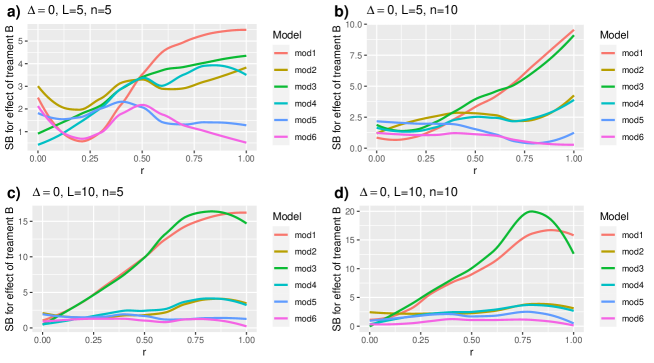
Figure 1: Standardized bias for the estimates of the effect of treatment B without a washout period ($\Delta=0$); a) five observations ($L=5$) per period and five experimental units ($n=5$) by sequence, b) five observations ($L=5$) per period and ten experimental units ($n=10$) by sequence, c) ten observations ($L=10$) per period and five experimental units ($n=5$) by sequence and d) ten observations ($L=10$) per period and ten experimental units ($n=10$) by sequence.

Assume that there is a dose-finding experiment $2\times 2$, with the doses and responses as shown in Table 3. The results of the simulation study were Figure 1 shows the standardized bias of the estimator of the effect of treatment B, that is when the dose is twice that of treatment A under each of the six adjusted models. In the four figures, the model with complex carryover effects (mod6) had a lower bias than the other five models when the value of $r$ is greater than 0.25, except in Figure 1 a) where this difference is less evident, due to the small number of experimental units. In Figure 1 c), it is observed that although there are few experimental units, as there are more observations per experimental unit per period, the model with complex carryover effects did behave better than the other five. However, it is worth clarifying that the model with simple carryover effects (but estimated with the semi-parametric methodology) had the worst performance than mod6, but better than the other 4 models. Finally, the models without carryover effects exhibited very bad behavior, and those that assumed complex carryover effects linearly or interaction with time do not have such high biases with respect to the semiparametric ones. As the value of $r$ increases, that is, the carryover effects become stronger, the model proposed by Cruz et al. (2023a) performed better than the others.

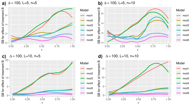
Figure 2: Standardized bias for the estimates of the effect of treatment B with one hundred times of washout period ($\Delta=100$); a) five observations ($L=5$) per period and five experimental units ($n=5$) by sequence, b) five observations ($L=5$) per period and ten experimental units ($n=10$) by sequence, c) ten observations ($L=10$) per period and five experimental units ($n=5$) by sequence and d) ten observations ($L=10$) per period and ten experimental units ($n=10$) by sequence

Looking at Figure 2, the washout period is too long and it is assumed that there are no carryover effects, but it is observed that the models without the estimation of the time effect had a large bias when the number of observations per period increased, this is because the treatment effect interacts non-linearly with time. Therefore, the proposed model is capable of detecting the change throughout the observation period when there are more than five observations per period, and because of that, it had a lower bias in all simulated values of $r$, and the model with simple carryover effects performed similarly to that with complex carryover effects
The figures in the supplementary material show that the model with complex carryover effects proposed here performed better in all scenarios where the number of measurements per period is greater than five. Behavior that is maintained regardless of the value of $r$ and the washout period, which brings evidence about the robustness of this model, in AB/BA designs.

3.2 Williams array with four treatments

The example given in Senn (1992) was adapted and consists of a crossover design with Williams array as shown in Table 5.

Sequence	Period 1	Period 2	Period 3	Period 4
BADC	L observations	L observations	L observations	L observations
CDAB	L observations	L observations	L observations	L observations
DBCA	L observations	L observations	L observations	L observations
ACBD	L observations	L observations	L observations	L observations

Table 5: Crossover design with Williams square

Suppose we have a dose-finding experiment using the Williams square, with the doses and responses shown in Table 3.

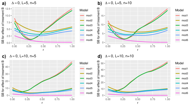
Figure 3: Standardized bias for the estimates of the effect of treatment B without a washout period ($\Delta=0$); a) five observations ($L=5$) per period and five experimental units ($n=5$) by sequence, b) five observations ($L=5$) per period and ten experimental units ($n=10$) by sequence, c) ten observations ($L=10$) per period and five experimental units ($n=5$) by sequence and d) ten observations ($L=10$) per period and ten experimental units ($n=10$) by sequence.

The effect of treatment B is $\beta$ according to Table 3. The simulations were run and the following results were obtained: Figure 3 shows the standardized bias of the treatment effect estimator B under each of the six models. It is observed that when the number of observations per period is equal to five, the proposed model had a lower bias than the other five regardless of the value of $r$. When the number of observations per period increased to 10 or 100 (observed in the graphs in the supplementary material), the model accounting for complex carryover effects had a lower bias at all values of $r$. Furthermore, the model with only treatment, period, and time effects behaved similarly to the model with only a constant simple carryover, which supports ideas discussed by Senn (1992) and Fleiss (1989). That is, if a complex carryover effect is not assumed, it is better to assume a simple carryover effect but estimate it nonparametrically. When comparing the figures with the AB/BA model, similar behavior of the models with complex carryover effects estimated as suggested by Cruz et al. (2023a) was obtained.

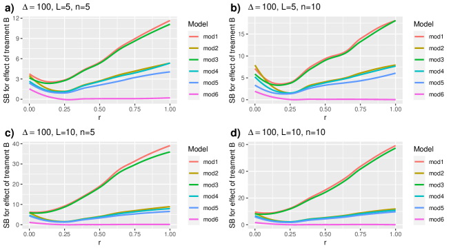
Figure 4: Standardized bias for the estimates of the effect of treatment B $\Delta=100$ (washout period); a) five observations ($L=5$) per period and five experimental units ($n=5$) by sequence, b) five observations ($L=5$) per period and ten experimental units ($n=10$) by sequence, c) ten observations ($L=10$) per period and five experimental units ($n=5$) by sequence and d) ten observations ($L=10$) per period and ten experimental units ($n=10$) by sequence

Looking at Figure 4, the washout period is too long and it is assumed that there are no carryover effects, but it is observed that the models without the time effect had a large bias when the number of observations per period increased, in the same way as explained in Figure 2. The figures in the supplementary material showed that the model with complex carryover effects proposed here is better in all scenarios where the number of measurements per period is greater than five. Behavior that is kept regardless of the value of $r$ and the washout period, again, is evidence supporting the robustness of this model.

4 Application

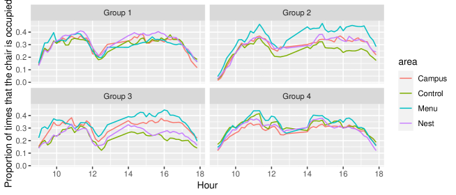
Figure 5: Proportions of times the chair is occupied over hours, the average of each treatment in each observation of the period is presented.

To see the behavior of the methodology in a Williams design with 96 observations for each experimental unit per period, the data obtained from the experiment described in Table 1 will be analyzed, and whose profile graph is shown in Figure 5. Several models will be fitted to the data set, assuming a logistic link and a binomial distribution, and interchangeable and independent correlation matrices will be explored (similar to a GLM). Regarding carryover effects, the following scenarios will be assumed: i) Without: that is, there are no carryover effects, ii) Linear: There are simple carryover effects and behave linearly in time, iii) Simple: These are assumed simple carryover and iv) complex: these are assumed complex carryover effects. Models will be compared using the quasi-likelihood criterion ($QIC$) and fitted with a semiparametric approach as described in Cruz et al. (2023a), using the CrossCarry package (Cruz et al., 2023c) of software R (R, 2023). The $QIC$ defined by Pan (2001) is:

$$QIC=-2QL(\hat{\boldsymbol{\mu}};\boldsymbol{I})+2trace(\hat{\boldsymbol{\Omega}}^{-1}_{I}\hat{\boldsymbol{V}}_{\boldsymbol{R}})$$ (7)

where $\hat{\mu}=\hat{\eta}=g^{-1}(x\hat{\boldsymbol{\beta}})$ is the estimated expected value for the observation with the model assuming the correlation matrix $\boldsymbol{R}$, $\hat{\boldsymbol{\Omega}}_{I}$ is the estimated variance matrix for vector $\boldsymbol{\beta}$ under a correlation matrix $\boldsymbol{R}(\boldsymbol{\alpha})=\mathbf{I}_{n_{i}}$, and $\hat{\boldsymbol{V}}_{\boldsymbol{R}}$ is the variance matrix estimated for the vector $\boldsymbol{\beta}$ assuming the correlation matrix $\boldsymbol{R}(\boldsymbol{\alpha})$. After fitting several models, the model with the lowest $QIC$ is selected because it is the one featuring the best balance between goodness of fit and complexity.

Model	Correlation	QIC
Complex	Autoregressive	2960.30
Complex	Independence	2908.11
Simple	Autoregressive	2949.12
Simple	Independence	2938.87
Linear	Autoregressive	58831.94
Linear	Independence	58773.25
Without	Autoregressive	58692.16
Without	Independence	58664.20

Table 6: QIC for the fitted models to the proportions of times that chair is occupied

The results of the QIC are presented in Table 6, and it has been observed that the semiparametric estimation with GEE yielded a lower QIC, and therefore a better performance. In addition, the carryover effect is complex and the correlation structure is independent. Furthermore, the reduction in the QIC is very large when assuming semiparametric time effects, and this is because it captures the functional form over time very well, which is very valuable in improving the estimation of the possible carryover effects and treatment effects. Therefore, the analysis is carried out with the model given by:

$$\ln\left(\frac{p_{i}}{1-p_{i}}\right) =\boldsymbol{x}_{ijk}^{T}\boldsymbol{\beta}+f_{1}(\boldsymbol{Z}_{ijk})+\sum_{c=2}^{13}f_{c}(\boldsymbol{Z}_{ijk})$$

where $\boldsymbol{x}_{ijk}$ is the matrix that contains the values of period and treatment, $\boldsymbol{Z}_{ijk}$ contains the measurement time instants within each period, $f_{1}$ is the function that describes the temporary effect, $f_{2}$ is the function that describes the carryover effect of A on B and $f_{13}$ is the carryover effect of D on C.

	Df	X2	P($>$$|$Chi$|$)
wave	3	10.97	0.0119
area	3	39.53	0.0000
Carry_Control	1	2.76	0.0968
Carry_Menu	1	0.18	0.6729
Carry_Nest	1	0.11	0.7368
minute	1	22.11	0.0000

Table 7: Deviance Analysis of proportions of times that chair is occupied using GEE usual with simplex carryover

Table 7 shows the deviance analysis for a usual GEE model with linear carryover effects over time, for the period and the treatment effects, where the significance of both effects is observed, using a Wald statistic; this is because according to Theorem 1, the parametric effects converge to a normal distribution.

	Df	X2	P($>$$|$Chi$|$)
Period	3	20.77	0.0001
area	3	18.75	0.0003

Table 8: Deviance Analysis of proportions of times that chair is occupied using GEE-splines

However, this model has a very high QIC, and Table 7 is shown to be able to compare with Table 8 and observe the differences of a poor specification of the carryover effects on the estimation of the treatment effects. Table 8 shows the deviance analysis for the period and treatment effects but assuming complex carryover effects under the model with the lowest QIC, significance of both effects is observed. According to the results obtained in this paper, a minor bias is expected from the results of Table 8.

	Estimate	Std.err	Wald	Pr($>$$|$W$|$)
(Intercept)	-1.9131	0.1513	159.7954	0.0000
Period 2	0.1620	0.1150	1.9823	0.1592
Period 3	0.5189	0.1273	16.6132	0.0000
Period 4	0.5187	0.1468	12.4809	0.0004
areaControl	-0.3134	0.1016	9.5177	0.0020
areaMenu	0.5299	0.0947	31.3127	0.0000
areaNest	-0.2820	0.1019	7.6570	0.0057
Carry_Control	-0.2025	0.1118	3.2775	0.0702
Carry_Menu	0.2413	0.1091	4.8879	0.0270
Carry_Nest	-0.5962	0.1058	31.7807	0.0000
minute	0.0573	0.0068	70.7556	0.0000

Table 9: Analysis of proportions of times that chair is occupied using GEE with simplex carryover

Tables 9 and 10 show the estimates, standard errors, Wald statistics, and p-values. Table 9 shows the output for the model with simple linear carryover effects and Table 10 shows the output for the model with complex carryover effects estimated by the GEE-splines methodology. A change is clearly observed in the estimated values and their standard error for each of the parameters; for example, the estimator of the Menu treatment effect goes from 0.5599 (se = 0.0947) with the simple carryover model to 0.0435 (se = 0.0151) with the complex carryover model. According to the results of this paper, the second estimator contains less bias and is, therefore, more useful for the researcher’s decisions.

	Estimate	Std.err	Wald	Pr($>$$|$W$|$)
(Intercept)	0.1540	0.0147	109.9372	0.0000
Period 2	-0.0380	0.0156	5.9187	0.0150
Period 3	-0.0195	0.0158	1.5192	0.2177
Period 4	-0.0657	0.0148	19.6944	0.0000
areaControl	-0.0183	0.0156	1.3793	0.2402
areaMenu	0.0435	0.0151	8.3659	0.0038
areaNest	-0.0036	0.0155	0.0537	0.8168

Table 10: Analysis of proportions of times that chair is occupied using GEE-splines

Additionally, Table 10 shows that the Menu treatment has a higher occupancy than the other three, which can be seen in the blue line in Figure 5. It is also observed that period 4 has a smaller estimate of occupation than the other three. Multiple comparisons could be made using a methodology such as Tukey or Bonferroni, since the estimate of the variance and covariance matrix of $\boldsymbol{\beta}$ is known.

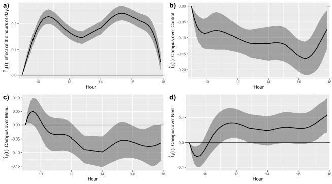
Figure 6: a) Estimate of $f_{1}$, i.e. change mean of proportions of times that chair, b) First order carryover effect of the treatment A over treatment B, b) First order carryover effect of the treatment A over treatment C, and d) First order carryover effect of the treatment A over treatment D. All figures present 95% confidence intervals and are based on the crossover design of Table 1 with complex carryover effects and estimated using splines.

With the results of Table 6, the semiparametric estimators of each of the 13 design functions are obtained, i.e. the temporal effect and the other effects. Figure 6.a) shows the estimated effect of time in the design, i.e., how the average occupancy of the work chairs behaves throughout the day throughout the experiment. There is a decrease in the hour 13 to 14, that is, when the workers go out for lunch and two maxima, which reflects the behavior observed empirically in Figure 5. Figure 6 b) shows the first-order carryover effect of the Campus treatment on Control. It shows a decreasing effect until 17 and then increases over time; therefore, having been in the Campus treatment a period ago causes people who receive the control treatment to occupy work chairs less frequently.

Figure 6 c) shows the first-order carryover effect of the Campus treatment on Menu. It is a sustained and negative decrease over time, very similar to that observed in Control, although it is smaller (close to 0), i.e., having been in the Campus treatment a period ago makes the people who receive the Menu treatment occupy work chairs less frequently. Figure 6 d) shows the first-order carryover effect of the Campus treatment on Nest. It is negative in the first hours and then presents a sustained and positive growth over time, different from that observed in the Control, which is why the carryover effects are not simple. In addition, people who received the Campus treatment just before the Nest treatment tend to have a higher frequency of occupancy of work chairs.

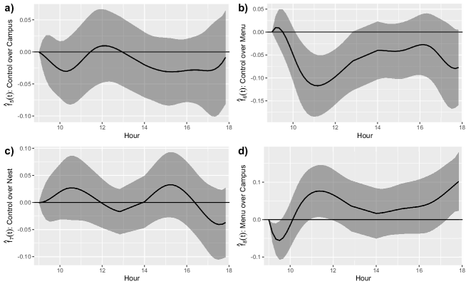
Figure 7: First order carryover effect of the treatment a) B over treatment A, b) B over treatment C, c) B over treatment D, and d) C over treatment A. All figures present 95% confidence intervals and are based on the crossover design of Table 1 with complex carryover effects and estimated using splines.

Figure 7 a) shows the first-order carryover effect of the Control on Campus treatment. Since it is not significant, it can be stated that there is no carryover effect present. Figure 7 b) shows the first-order carryover effect of the Control over Menu treatment. It is a sustained and negative decrease over time in the first few hours and then becomes non-significant, that is, having been in the Control treatment for a period of time causes people who receive the Menu treatment to occupy work chairs less frequently in the early hours of the day.

Figure 7 c) shows the first-order carryover effect of the Control treatment in Nest. Since it is not significant, it can be stated that there is no carryover effect present. If we compare the first-order carryover effects of the control treatment over the others, they are smaller than those of the Campus treatment. Figure 7 d) shows the first-order carryover effect of the Menu treatment on Campus. It presents persistent and positive growth over time; therefore, having received the Menu treatment a period ago, causes workers to occupy the chair more times in the Campus treatment.

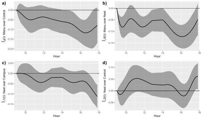
Figure 8: First order carryover effect of the treatment a) C over treatment B, b) C over treatment D, c) D over treatment A, and d) D over treatment B. All figures present 95% confidence intervals and are based on the crossover design of Table 1 with complex carryover effects and estimated using splines

Figure 8 a) shows the first-order carryover effect of the Menu treatment in Control. It is a carryover effect that decreases over time; therefore, having received the Menu treatment in the previous period causes workers who receive the control treatment to occupy jobs less often and this behavior increases as the day progresses. Figure 8 b) shows the first-order carryover effect of the Menu treatment on Nest. It is a negative value over time, that is, having been in the Menu treatment in the previous period causes people who receive the Nest treatment to occupy work chairs less frequently.

Figure 8 c) shows the first-order carryover effect of the Nest treatment on Campus and Figure 8 d) shows the first-order carryover effect of the Nest treatment on Control. Both are not significant, it can be stated that there is no carryover effect. If we compare the first-order carryover effects of the control treatment over the others, these are smaller than those of the Campus and Menu treatments.

5 Conclusions

The discussion on complex carryover effects is long-standing in the field of statistics in clinical and human research, and so far, there has been no methodology that would allow consistent estimation of complex carryover effects. Perhaps, this is why these effects were ignored in many studies, either assuming that they did not exist or including simple carryover effects in the model. The first assumption was supported by some studies from pharmacology, while the second assumption was defended by statisticians and justified by the search for mathematical tractability but not by practical or empirical reasons. Having developed a methodology able to estimate these effects, strengthens the model used to analyze crossover designs. Here it was found that this estimate has a lower bias for the treatment effects, in scenarios where there is a complex carryover effect, which opens a path to close the discussion on whether or not to assume carryover effects. The only requirement is to have at least 5 observations for each experimental unit per period, which was supported theoretically and empirically (simulation study). Furthermore, in the real data application, the usefulness of the proposed methodology was evident. Beyond being treated as nuisance parameters, accounting for complex carryover effects may contribute to a better understanding of the studied phenomenon and lead to a more effective treatment design.

6 Supplementary files

• Supplementary file 1: A PDF file with plots of the $SB$ and the $RMSE$ for different combinations of parameters in the simulation AB/BA design and Williams Square.

• Supplementary file 2: A PDF file with plots of the $SB$ and the $RMSE$ for different combinations of parameters in the simulation Williams Square.

• Supplementary file 3: An R code with the simulation exercise and the analysis of the data of work environment levels

References

- Hinkelmann and Kempthorne (2005) Hinkelmann, K. & Kempthorne, O. Design and Analysis of Experiments. (Wiley,2005)
- Cruz et al. (2023a) Cruz, N.A, Melo, O.O & Martinez, C.A. Semiparametric generalized estimating equations for repeated measurements in cross-over designs. Statistical Methods In Medical Research. 32, 1033-1050 (2023)
- Cruz et al. (2023b) Cruz, N.A., Melo, O.O. & Martinez, C.A. A correlation structure for the analysis of Gaussian and non-Gaussian responses in crossover experimental designs with repeated measures. Statistical Papers. pp. 1-28 (2023)
- Vegas et al. (2016a) Vegas, S., Apa, C. & Juristo, N. Crossover designs in software engineering experiments: Benefits and perils. IEEE Transactions On Software Engineering. 42, 120-135 (2016)
- Fleiss (1989) Fleiss, J. A critique of recent research on the two-treatment crossover design. Controlled Clinical Trials. 10, 237-243 (1989)
- Senn (1992) Senn, S. Is the ‘simple carry-over’model useful?. Statistics In Medicine. 11, 715-726 (1992)
- Basu and Santra (2010) Basu, S. & Santra, S. A joint model for incomplete data in crossover trials. Journal Of Statistical Planning And Inference. 140, 2839-2845 (2010)
- Josephy et al. (2015) Josephy, H., Vansteelandt, S., Vanderhasselt, M. & Loeys, T. Within-subject mediation analysis in AB/BA crossover designs. The International Journal Of Biostatistics. 11, 1-22 (2015)
- Hao et al. (2015) Hao, C., Rosen, D. & Rosen, T. Explicit influence analysis in two-treatment balanced crossover models. Mathematical Methods Of Statistics. 24, 16-36 (2015)
- Lui (2015) Lui, K. Test equality between three treatments under an incomplete block crossover design. Journal Of Biopharmaceutical Statistics. 25, 795-811 (2015)
- Rosenkranz (2015) Rosenkranz, G. Analysis of cross-over studies with missing data. Statistical Methods In Medical Research. 24, 420-433 (2015)
- Grayling et al. (2018) Grayling, M., Mander, A. & Wason, J. Blinded and unblinded sample size reestimation in crossover trials balanced for period. Biometrical Journal. 60, 917-933 (2018)
- Madeyski and Kitchenham (2018) Madeyski, L. & Kitchenham, B. Effect sizes and their variance for AB/BA crossover design studies. Empirical Software Engineering. 23, 1982-2017 (2018)
- Kitchenham et al. (2018) Kitchenham, B., Madeyski, L., Curtin, F. & Others Corrections to effect size variances for continuous outcomes of cross-over clinical trials. Statistics In Medicine. 37, 320-323 (2018)
- Oh et al. (2003) Oh, H., Ko, S. & Oh, M. A Bayesian approach to assessing population bioequivalence in a 2x2x2 crossover design. Journal Of Applied Statistics. 30, 881-891 (2003)
- Curtin (2017) Curtin, F. Meta-analysis combining parallel and crossover trials using generalised estimating equation method. Research Synthesis Methods. 8, 312-320 (2017)
- Li et al. (2018) Li, F., Forbes, A., Turner, E. & Preisser, J. Power and sample size requirements for GEE analyses of cluster randomized crossover trials. Statistics In Medicine. (2018)
- Jankar and Mandal (2021) Jankar, J. & Mandal, A. Optimal Crossover Designs for Generalized Linear Models: An Application to Work Environment Experiment. Statistics And Applications. 19, 319-336 (2021)
- Pitchforth et al. (2020) Pitchforth, J., Nelson-White, E., Helder, M. & Oosting, W. The work environment pilot: An experiment to determine the optimal office design for a technology company. PloS One. 15, e0232943 (2020)
- Jankar et al. (2020) Jankar, J., Mandal, A. & Yang, J. Optimal crossover designs for generalized linear models. Journal Of Statistical Theory And Practice. 14, 1-27 (2020)
- Harville (1997) Harville, D. Matrix algebra from a statistician’s perspective. (Springer,1997)
- Harezlak et al. (2016) Harezlak, J., Ruppert, D. & Wand, M. Semiparametric regression in R. (Springer, 2016)
- Cruz et al. (2023c) Cruz, N.A., López Pérez, L.A. & Melo, O.O. Analysis of cross-over experiments with count data in the presence of carry-over effects. Statistica Neerlandica. 77, 516-542 (2023)
- R (2023) R Core Team R: A Language and Environment for Statistical Computing. (R Foundation for Statistical Computing, 2024), https://www.R-project.org/
- Jones and Kenward (2015) Jones, B. & Kenward, M. Design and Analysis of Cross-Over Trials Third Edition. (Chapman & Hall/CRC, 2015)
- Pan (2001) Pan, W. Akaike’s information criterion in generalized estimating equations. Biometrics. 57 pp. 120-125 (2001)