C-GAIL: Stabilizing Generative Adversarial
Imitation Learning with Control Theory
Abstract
Generative Adversarial Imitation Learning (GAIL) trains a generative policy to mimic a demonstrator. It uses on-policy Reinforcement Learning (RL) to optimize a reward signal derived from a GAN-like discriminator. A major drawback of GAIL is its training instability – it inherits the complex training dynamics of GANs, and the distribution shift introduced by RL. This can cause oscillations during training, harming its sample efficiency and final policy performance. Recent work has shown that control theory can help with the convergence of a GAN’s training. This paper extends this line of work, conducting a control-theoretic analysis of GAIL and deriving a novel controller that not only pushes GAIL to the desired equilibrium but also achieves asymptotic stability in a ‘one-step’ setting. Based on this, we propose a practical algorithm ‘Controlled-GAIL’ (C-GAIL). On MuJoCo tasks, our controlled variant is able to speed up the rate of convergence, reduce the range of oscillation and match the expert’s distribution more closely both for vanilla GAIL and GAIL-DAC.
1 Introduction
Generative Adversarial Imitation Learning (GAIL) (Ho & Ermon, 2016) is a technique for learning a decision-making policy in a sequential environment by imitating trajectories collected from an expert demonstrator. GAIL follows the Generative Adversarial Network (GAN) (Goodfellow et al., 2014) template, with a learned policy serving as the generator network, and a discriminator network classifying expert trajectories from generated trajectories. The learned policy is optimized by Reinforcement Learning (RL) with a reward signal derived from the discriminator. This paradigm offers distinct advantages over other imitation learning strategies such as Inverse Reinforcement Learning (IRL), which requires an explicit model of the reward function (Ng et al., 2000), and Behavior Cloning (BC), which suffers from a distribution mismatch during roll-outs (Codevilla et al., 2019).
However, GAIL does bring certain challenges. One key issue it inherits from GANs is instability during training (Mescheder et al., 2018). This problem, while theoretically manageable in linear settings (Zhang et al., 2020; Guan et al., 2021), manifests in practice as oscillating training curves and an inconsistency in matching the expert’s performance.
This paper addresses this issue by drawing on recent advancements studying GANs with control theory (Xu et al., 2020; Luo et al., 2023) to improve the stability and convergence properties of GAIL. We first show how GAIL’s training dynamics can be expressed as a system of differential equations (Section 3). This surprisingly reveals that the desirable minimax point is not an equilibrium of GAIL. In response, we propose a ”one-step GAIL” setting, and design a controller that does create an equilibrium at the desired point (Section 4). We theoretically prove that this controller allows the dynamical system of GAIL’s training to achieve asymptotic stability.
Motivated by this, we propose C-GAIL, which incorporates a pragmatic controller that can be added as a regularization term to the loss function in practice. We verify the effectiveness of our method on experiments run across a suite of MuJoCo control tasks (Section 5).
Concretely, we offer several contributions.
-
•
We provide the first analysis of GAIL as a dynamical system from the perspective of control theory.
-
•
We identify an issue with convergence of GAIL, showing that the desired state is not an equilibrium point.
-
•
We propose a simplified ”one-step GAIL” model, where we design a controller that we theoretically prove is asymptotically stable.
-
•
Based on this ideal controller, we propose a practical objective function for the discriminator, resulting in our C-GAIL algorithm.
-
•
Empirically we find that our method speeds up the convergence rate and reduces the range of oscillation in the return curves, and matches the expert’s distribution more closely on GAIL-DAC.
1.1 Related Work
Adversarial imitation learning. Inspired by GANs and inverse RL, Adversarial Imitation Learning (AIL) has emerged as a popular technique to learn from demonstrations. GAIL (Ho & Ermon, 2016) formulated the problem as matching an occupancy measure under the maximum entropy RL framework, with a a discriminator providing the policy reward signal, bypassing the need to recover the expert’s reward function. Several advancements were subsequently proposed to enhance performance and stability. AIRL (Fu et al., 2017) replaced the Shannon-Jensen divergence of GAIL by KL divergence. Baram et al. (2017) explored combining GAIL with model-based reinforcement learning. DAC (Kostrikov et al., 2018) utilized a replay buffer to remove the need for importance sampling and address the issue of absorbing states. Meanwhile, the stability of AIL has also been investigated from more of a theoretical standpoint. Chen et al. (2020) showed that GAIL approaches a stationary point (though this may not be the optimal solution) with a gradient-based algorithm in a general Markov Decision Process (MDP). Zhang et al. (2020) introduced a natural policy gradient (NPG) algorithm, showing it converges, sub-linearly, to the global optimal. Guan et al. (2021) extended the convergence analysis to non-linear MDPs. By contrast, our work begins from the novel perspective of dynamical systems, applied to the MDP setting, and is asymptotically stable with a smaller radius of convergence.
Control theory in adversarial learning. Control theory has recently emerged as a promising technique for studying adversarial learning in the supervised learning setting. Xu et al. (2020) designed a linear controller which offers GANs local stability. Luo et al. (2023) utilized a Brownian motion controller which was shown to offer GANs global exponential stability. Both works analyze the stability of GANs’ training with respect to their induced dynamical systems under linear simplified Dirac-GANs setting, and they extend the designed controllers from Dirac-GANs to normal GANs. However, for GAIL, the policy generator involves a MDP transition, which makes controllers from prior work inapplicable. Our work adopts this control theoretic perspective in a new setting – we must deal with both a non-linear dynamical system, and an induced distribution of a policy acting in an MDP rather than a static data distribution of supervised learning.
2 Preliminaries
In this section, we formally introduce our problem setting, then provide established definitions and theorems relating to the stability of dynamical systems represented by Ordinary Differential Equations (ODE’s).
2.1 Problem Setting
Consider a Markov Decision Process (MDP), described by the tuple , where is the state space, is the action space, is the transition probability function, is the reward function, is the probability distribution of the initial state , and is the discount factor. We work on the -discounted infinite horizon setting, and define the expectation with respect to a policy as the (discounted) expectation over the trajectory it generates. For some arbitrary function we have , where , , . Note that we use to represent the environment timestep, reserving to denote the training timestep of GAIL. For a policy , We define its (unnormalized) occupancy measure as and marginal function . We denote and the advantage function . We assume the setting where we are given a dataset of trajectories consisting of state-action tuples, collected from an expert policy . We assume access to interact in the environment in order to learn a policy , but do not make use of any external reward signal (except during evaluation).
2.2 Dynamical Systems and Control Theory
In this paper, we consider dynamical systems represented by an ODE of the form
| (1) |
where represents some property of the system, refers to the timestep of the system and is a function. One important question in dynamical systems, is whether the solution trajectory converges to some steady state value. A necessary condition for convergence is the existence of an ‘equilibrium’.
Definition 2.1.
Remark 2.2.
A dynamical system is unable to converge if an equilibrium does not exist.
A second important property of dynamical systems is ‘stability’. The stability of a dynamical system can be described with Lyapunov stability criteria. More formally, suppose is a solution trajectory of the above system (1) with equilibrium , we define two types of stability.
Definition 2.3.
Definition 2.4.
Remark 2.5.
A dynamical system can be Lyapnuov stable but not asymptotic stable. However, every asymptotic stable dynamical system is Lyapnuov stable.
The field of control theory has studied how to drive dynamical systems to desired states. This can be achieved through the addition of a ‘controller’ to allow influence over the dynamical system’s evolution, for example creating an equilibrium at some desired state, and making the dynamical system stable around it.
Definition 2.6.
(Controller) (Brogan, 1991) A controller of a dynamical system is a function such that
| (2) |
The equilibrium and stability criteria introduced for dynamical system (1), equally apply to this controlled dynamical system (2). In order to analyze the stability of a controller of the controlled dynamical system given an equilibrium , the following result will be useful.
Theorem 2.7.
Corollary 2.8.
If has positive determinant and negative trace, all its eigenvalues have negative real parts. Therefore theorem 2.7 also holds.
3 Analyzing GAIL as a Dynamical System
This section derives the differential equations governing the training process of GAIL, framing it as a dynamical system. Then, we analyze the convergence of the vanilla GAIL and find the vanilla GAIL is unable to converge to desired equilibrium due to the entropy term.
3.1 GAIL Dynamics
GAIL consists of a learned generative policy and a discriminator . The discriminator estimates the probability that an input state-action pair is from the expert policy, rather than the learned policy. GAIL alternatively updates the policy and discriminator parameters, and . (The parameter subscripts are subsequently dropped for clarity.) The original GAIL objective (Ho & Ermon, 2016) is,
| (3) |
where is the expert demonstrator policy, is the learned policy, and is its entropy. Respectively, the objective functions for the discriminator and policy can be written,
| (4) | ||||
To describe GAIL as a dynamical system, we write how its two components evolve over the training timestep . In this work, we directly consider the updates of and in their respective function spaces. The objective in Eq. (4) can be optimized in function space using gradient based method,
| (5) | ||||
where is the learning rate and the discrete iteration number. In the continuous-time limit (‘gradient flow’), Eq. (5) can be represented by the functional derivative,
Formally, we consider the evolution of the discriminator function and the policy generator over time . Moreover, define to be the discriminator function and to be the policy generator evaluated at the state-action pair respectively.
Since the demonstrator policy is constant through the training dynamic, we omit dependence on . We derive these functional derivatives in Appendix Lemma A.2, which take the form,
| (6) | |||
| (7) |
where and are occupancy measure and advantage function under the policy , defined in Section 2.1. We slightly abuse notation with meaning the state-only occupancy .
3.2 On the Convergence of GAIL
The desirable outcome of the GAIL training process, is for the learned policy to perfectly match the expert policy, and the discriminator to be unable to distinguish between the expert and learned policy. This desired state is defined as,
Definition 3.1.
(Desired state) We define the desired outcome of the GAIL training process as the discriminator and policy reaching the following,
| (8) | |||
| (9) |
We are interested in whether this desired state is an equilibrium of the dynamical system described by Eq. (6) & (7). According to Def. 2.1, the dynamical system should equal zero at this point, but according to Proposition A.3 and A.5, we find,
| (10) | |||
| (11) |
Hence, the desired state is not an equilibrium, and GAIL will not converge to it (Remark 2.2). One can find that it is due to the entropy term in GAIL’s objective that Eq. (11) is not equal to zero – Corollary A.4.
4 Controlled GAIL
Having shown in Section 3 that GAIL does not converge to the desired state, this section considers adding a controller so that it does. We propose ”one-step GAIL”, which we analyze the training dynamic for one environment timestep. We design controllers for both the discriminator and the policy. We show that this controlled system converges to the desired equilibrium and also achieves asymptotic stability. We then propose a pragmatic variant of this controller to be used in practise which we name C-GAIL.
4.1 Controlling the Training Process of GAIL
To design a controller for GAIL, we consider a single environment timestep of the trajectory with state and action – we refer to this as the ‘one-step GAIL’ model. Let be the probability of the state at on timestep . The objectives for the discriminator and the policy can then be written,
| (12) |
The dynamical system of these functions is written,
| (13) |
| (14) |
Notice that though Eq. (13) & (14) are ODEs of functions and respectively, the dynamics of and for each pair are independent. Therefore, we can decompose Eq. (13) & (14) into a series of ODEs, each for a particular pair, and analyze the stability of this system of ODEs of for each pair individually, and conclude that for each given pair, our controller is able to asymptotically stabilize its dynamical system.
We now consider the stability of a system of ODEs for two scalar variables , rather than functions. With given, we simplify the notation as , , , , and rewrite our dynamical system,
| (15) | |||
| (16) |
We showed earlier that the GAIL dynamic in Eq. (6) & (7) does not converge to the desired state. We now consider the addition of controllers to push our dynamical system to the desired stated. Specifically, we consider linear negative feedback control (Boyd & Barratt, 1991), which can be applied to a dynamical system to reduce its oscillation. We specify our controlled GAIL system as,
| (17) | |||
| (18) |
where and are the controllers to be designed for the discriminator and policy respectively. Since the derivative of the discriminator with respect to time evaluated at the desired state in Eq. (10) already equals zero, the discriminator is already able to reach its desired state. Nevertheless, the discriminator can still benefit from a controller to speed up the rate of convergence – we choose a linear negative feedback controller for to push the discriminator towards its desired state. On the other hand, the derivative of the policy generator evaluated at its desired state in Eq. (16) does not equal zero. Therefore, should be set to make Eq. (18) equal to zero evaluated at the desired state. We have designed it to cancel out all terms in Eq. (16) at this desired state, and also provide feasible hyperparameter values for an asymptotically stable system. Hence, we select and to be the following functions,
| (19) | |||
| (20) |
where are hyper-parameters. Intuitively, as gets larger, the discriminator will be pushed harder towards the optimal value of . This means the discriminator would converge at a faster speed but may also have a larger radius of oscillation. To understand the convergence behavior of this controlled dynamical system, and provide bounds on the values of & , we will analyze its stability in the next section.
4.2 Analyzing the Stability of Controlled GAIL
In this section, we apply Theorem 2.7 to formally prove that the controlled GAIL dynamical system described in Eq. (17) & (18) is asymptotically stable (Def. 2.4) and give bounds with and .
For simplicity, let us define , and a function such that is the vector,
| (21) |
Therefore, our controlled training dynamic of GAIL in Eq. (17) and Eq. (18) can be transformed to the following vector form
| (22) |
Given this set up, we prove in Appendix B that the following theorem holds.
Theorem 4.1.
Assumption 4.2.
We assume , and,
| (a) | |||
| (b) |
Proof sketch. The first step in proving asymptotic stability of the system in Eq. (22), is to verify whether our desired state is an equilibrium (Def. 2.1). We substitute the desired state, , into system (22) and verify,
We then find the linearized system about the desired state,
Under Assumption 4.2, we show that and . Finally we invoke Theorem 2.7 and Corollary 2.8 to conclude that the system in Eq. (22) is asymptotically stable.
4.3 From Controller to Loss Function
Even though we analyzed our controllers in the simplified setting of Section 4.1, we would like to extend our controller to be incorporated into the objective functions of GAIL. The controllers in Eq. 19 & 20 are designed to make GAIL’s training dynamic converge to the desired state. Since they are defined in the dynamical system setting, we need to integrate these with respect to time, in order to recover an objective function that can be practically optimized by a GAIL algorithm. In this section, we extend our controller from ”one-step GAIL” back to normal GAIL’s setting and convert our controller as a regularization term to the original loss functions and propose C-GAIL, a controlled GAIL algorithm, to stabilize the training process of GAIL.
We note that whilst our theoretical guarantees may not hold in the pragmatic version, this follows a precedent for designing stable GAN variants. For example, Xu et al. (2020); Luo et al. (2023) proposed their controller in the simplified linear Dirac-GAN (Mescheder et al., 2018) model, which guided them to design practical algorithms that perform well empirically despite falling outside of the simplified setting.
Recalling that and are the original GAIL loss functions for the discriminator and policy (Eq. (4)), we define and as modified loss functions with the integral of our controller applied, such that
| (23) | ||||
| (24) | ||||
While can be implemented directly, the inclusion of , the expert policy, in is problematic – the very goal of the algorithm is to recover this, and we do not have access to it before training! Hence, in our practical implementations, we use our modified loss to update the discriminator, but the original unmodified policy objective for the policy. This results in the C-GAIL Algorithm 1.
Our algorithm results in the addition of a regularization term to the discriminator to control and speed up its rate of convergence. Hence, it is also compatible with other variants of GAIL, by straightforwardly incorporating it into their discriminator objective function. Empirically we find that our algorithm is effective in GAIL variants such as GAIL-DAC. Evaluations follow in Section 5.
| Ant | Half Cheetah | Hopper | Swimmer | Walker2d | |
|---|---|---|---|---|---|
| Random | |||||
| Expert | |||||
| Controlled GAIL | |||||
| GAIL | |||||
| BC | |||||
| AIRL | |||||
| DAgger |
5 Evaluation
This section evaluates the benefit of integrating the controller developed in Section 4 with popular variants of GAIL. We test the algorithms on their ability to imitate an expert policy in simulated continuous control problems in MuJoCo (Todorov et al., 2012). Specifically, we consider applying our controller to two popular GAIL algorithms – both the original ‘vanilla’ GAIL (Ho & Ermon, 2016) and also GAIL-DAC (Kostrikov et al., 2018), a state-of-the-art variant which uses a discriminator-actor-critic (DAC) to improve sample efficiency and reduce the bias of the reward function.
5.1 Experimental Setup
We incorporate our controller in vanilla GAIL and GAIL-DAC, naming our controlled variants C-GAIL and C-GAIL-DAC. We leverage the implementations of Gleave et al. (2022) (vanilla GAIL) and Kostrikov et al. (2018) (GAIL-DAC). Gleave et al. (2022) also provide other common imitation learning frameworks – BC, AIRL, vanilla GAIL, and dataset aggregation (DAgger) (Ross et al., 2011) – which we also compare to.
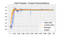
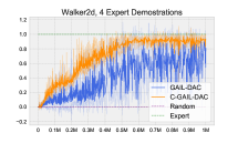
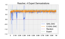
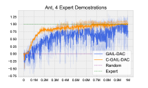
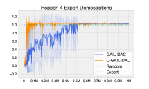
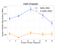
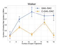
For C-GAIL-DAC, we test five MuJuCo environments: Half-Cheetah, Ant, Hopper, Reacher and Walker 2D. Our experiments follow the same settings as Kostrikov et al. (2018). The discriminator architecture has a two-layer MLP with 100 hidden units and tanh activations. The networks are optimized using Adam with a learning rate of , decayed by every gradient steps. We vary the number of provided expert demonstrations: , though unless stated we report results using four demonstrations. We assess the normalized return over training for GAIL-DAC and C-GAIL-DAC to evaluate their speed of convergence and stability, reporting the mean and standard deviation over five random seeds. The normalization is done with 0 set to a random policy’s return and 1 to the expert policy return.
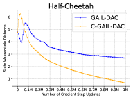
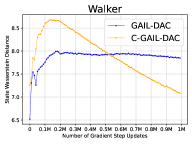
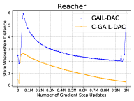
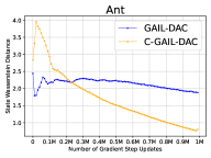
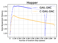
In addition to recovering the expert’s return, we are also interested in how the closely expert’s state distribution is matched, for which we use the state Wasserstein (Pearce et al., 2023). This requires empirical samples from two distributions, collected by rolling out the expert and learned policy for 100 trajectories each. We then use the POT library’s ‘emd2’ function (Flamary et al., 2021) to compute the Wasserstein distance, using the L2 cost function with a uniform weighting across samples.
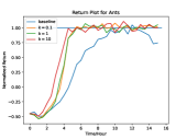
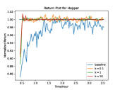
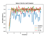
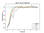
To evaluate C-GAIL, we follow the experimental protocol from Gleave et al. (2022), both for GAIL and other imitation learning baselines. These are evaluated on Ant, Hopper, Swimmer, Half-Cheetah and Walker 2D. For C-GAIL, we change only the loss and all other GAIL settings are held constant. We assess performance in terms of the normalized return. We use this set up to ablate a key hyperparameter of C-GAIL, varying .
5.2 Results
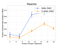
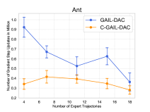
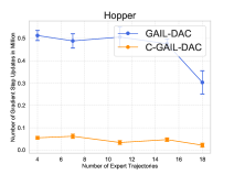
We compare GAIL-DAC to C-GAIL-DAC in Figure 1 (return), 2 (state Wasserstein), and 3 (convergence speed). Figure 1 shows that C-GAIL-DAC speeds up the rate of convergence and reduces the oscillation in the return training curves across all environments. For instance, on Hopper, C-GAIL-DAC converges 5x faster than GAIL-DAC with less oscillations. On Reacher, the return of GAIL-DAC continues to spike even after matching the expert return, but this does not happen with C-GAIL-DAC. On Walker 2D, the return of GAIL-DAC oscillates throughout training, whereas our method achieves a higher return at has reduced the range of oscillation by more than 3 times. For Half-Cheetah, our method converges 2x faster than GAIL-DAC. For Ant environment, C-GAIL-DAC reduces the range of oscillations by around 10x.
In addition to matching the expert’s return faster and with more stability, Figure 2 shows that C-GAIL-DAC also more closely matches the expert’s state distribution than GAIL-DAC, with the difference persisting even towards the end of training for various numbers of expert trajectories. Toward the end of training, the state Wasserstein for C-GAIL-DAC is more than 2x smaller than the state Wasserstein for GAIL-DAC on all five environments.
Figure 3 shows that these improvements hold for differing numbers of provided demonstrations. It plots the number of gradient steps for GAIL-DAC and C-GAIL-DAC to reach of the max-return for vaious numbers of expert demonstrations. Our method is able to converge faster than GAIL-DAC regardless of the number of demonstrations.
Hyperparameter sensitivity. We evaluate the sensitivity to the controller’s hyperparameter using vanilla GAIL. Figure 4 (Appendix C) plots normalized returns. For some environments, minor gains can be found by tuning this hyperparameter, though in general for all values tested, the return curves of C-GAIL approach the expert policy’s return earlier and with less oscillations than GAIL.
Other imitation learning methods. Table 1 benchmarks C-GAIL against other imitation learning methods, including BC, AIRL, and DAgger, some of which have quite different requirements to the GAIL framework. The table shows that C-GAIL is competitive with many other paradigms, and in consistently offers the lowest variance between runs of any method.
6 Discussion & Conclusion
This work helped understand and address the issue of training instability in GAIL, using the lens of control theory, which has recently been proven affective when applied to other adversarial learning frameworks. We formulated GAIL’s training as a dynamical system and designed a controller that stabilizes it at the desired equilibrium, encouraging convergence to this point. We showed theoretically that our controlled system achieves asymptotic stability. In practise, we found it reached the expert return both faster and with less oscillation than the uncontrolled variants, and also matched the expert’s state distribution more closely.
Whilst our controller theoretically converges to the desired equilibrium, and empirically stabilizes training, we recognize several limitations of our work. In our description of GAIL training as a continuous dynamical system, we do not account for the updating of generator and discriminator being discrete as in practice. In our practical implementation of the controller, we only apply the portion of the loss function acting on the discriminator, since the generator portion requires knowing the likelihood of an action under the expert policy (which is precisely what we aim to learn!). We leave it to future work to explore whether estimating the expert policy and incorporating a controller for the policy generator brings benefit.
7 Broader impact
This work has provided an algorithmic advancement in imitation learning. As such, we have been cognisant of various issues such as those related to learning from human demonstrators – e.g. privacy issues when collecting data. However, this work avoids such matters by using trained agents as the demonstrators. More broadly, we see our work as a step towards more principled machine learning methods providing more efficient and stable learning, which we believe in general has a positive impact.
References
- Baram et al. (2017) Baram, N., Anschel, O., Caspi, I., and Mannor, S. End-to-end differentiable adversarial imitation learning. In International Conference on Machine Learning, pp. 390–399. PMLR, 2017.
- Boyd & Barratt (1991) Boyd, S. P. and Barratt, C. H. Linear controller design: limits of performance, volume 7. Citeseer, 1991.
- Brogan (1991) Brogan, W. L. Modern control theory. Pearson education india, 1991.
- Chen et al. (2020) Chen, M., Wang, Y., Liu, T., Yang, Z., Li, X., Wang, Z., and Zhao, T. On computation and generalization of generative adversarial imitation learning. arXiv preprint arXiv:2001.02792, 2020.
- Codevilla et al. (2019) Codevilla, F., Santana, E., López, A. M., and Gaidon, A. Exploring the limitations of behavior cloning for autonomous driving. In Proceedings of the IEEE/CVF International Conference on Computer Vision, pp. 9329–9338, 2019.
- Flamary et al. (2021) Flamary, R., Courty, N., Gramfort, A., Alaya, M. Z., Boisbunon, A., Chambon, S., Chapel, L., Corenflos, A., Fatras, K., Fournier, N., et al. Pot: Python optimal transport. The Journal of Machine Learning Research, 22(1):3571–3578, 2021.
- Fu et al. (2017) Fu, J., Luo, K., and Levine, S. Learning robust rewards with adversarial inverse reinforcement learning. arXiv preprint arXiv:1710.11248, 2017.
- Gleave et al. (2022) Gleave, A., Taufeeque, M., Rocamonde, J., Jenner, E., Wang, S. H., Toyer, S., Ernestus, M., Belrose, N., Emmons, S., and Russell, S. imitation: Clean imitation learning implementations. arXiv preprint arXiv:2211.11972, 2022.
- Glendinning (1994) Glendinning, P. Stability, instability and chaos: an introduction to the theory of nonlinear differential equations. Cambridge university press, 1994.
- Goodfellow et al. (2014) Goodfellow, I., Pouget-Abadie, J., Mirza, M., Xu, B., Warde-Farley, D., Ozair, S., Courville, A., and Bengio, Y. Generative adversarial nets. Advances in neural information processing systems, 27, 2014.
- Guan et al. (2021) Guan, Z., Xu, T., and Liang, Y. When will generative adversarial imitation learning algorithms attain global convergence. In International Conference on Artificial Intelligence and Statistics, pp. 1117–1125. PMLR, 2021.
- Ho & Ermon (2016) Ho, J. and Ermon, S. Generative adversarial imitation learning. Advances in neural information processing systems, 29, 2016.
- Ince (1956) Ince, E. L. Ordinary differential equations. Courier Corporation, 1956.
- Kostrikov et al. (2018) Kostrikov, I., Agrawal, K. K., Dwibedi, D., Levine, S., and Tompson, J. Discriminator-actor-critic: Addressing sample inefficiency and reward bias in adversarial imitation learning. arXiv preprint arXiv:1809.02925, 2018.
- La Salle (1976) La Salle, J. P. The stability of dynamical systems. SIAM, 1976.
- Luo et al. (2023) Luo, T., Zhu, Z., Chen, J., and Zhu, J. Stabilizing gans’ training with brownian motion controller. arXiv preprint arXiv:2306.10468, 2023.
- Mescheder et al. (2018) Mescheder, L., Geiger, A., and Nowozin, S. Which training methods for gans do actually converge? In International conference on machine learning, pp. 3481–3490. PMLR, 2018.
- Ng et al. (2000) Ng, A. Y., Russell, S., et al. Algorithms for inverse reinforcement learning. In Icml, volume 1, pp. 2, 2000.
- Pearce et al. (2023) Pearce, T., Rashid, T., Kanervisto, A., Bignell, D., Sun, M., Georgescu, R., Macua, S. V., Tan, S. Z., Momennejad, I., Hofmann, K., et al. Imitating human behaviour with diffusion models. arXiv preprint arXiv:2301.10677, 2023.
- Ross et al. (2011) Ross, S., Gordon, G., and Bagnell, D. A reduction of imitation learning and structured prediction to no-regret online learning. In Proceedings of the fourteenth international conference on artificial intelligence and statistics, pp. 627–635. JMLR Workshop and Conference Proceedings, 2011.
- Todorov et al. (2012) Todorov, E., Erez, T., and Tassa, Y. Mujoco: A physics engine for model-based control. In 2012 IEEE/RSJ international conference on intelligent robots and systems, pp. 5026–5033. IEEE, 2012.
- Xu et al. (2020) Xu, K., Li, C., Zhu, J., and Zhang, B. Understanding and stabilizing gans’ training dynamics using control theory. In International Conference on Machine Learning, pp. 10566–10575. PMLR, 2020.
- Zhang et al. (2020) Zhang, Y., Cai, Q., Yang, Z., and Wang, Z. Generative adversarial imitation learning with neural network parameterization: Global optimality and convergence rate. In International Conference on Machine Learning, pp. 11044–11054. PMLR, 2020.
Appendix A Appendix A
| (25) | |||
| (26) |
Lemma A.1.
Given that is a parameterized policy. Define the training objective for entropy-regularized policy optimization as
Its gradient satisfies
where and are defined as
Proof.
The above derivation suggests that we can view the entropy term as an additional fixed reward . Applying the Policy Gradient Theorem, we have
where is similar to the classic Q-function but with an extra “entropy reward” term. ∎
Lemma A.2.
The functional derivatives for the two optimization objectives
respectively satisfy
where follows the same definition as in Lemma A.1.
Proof.
Regarding , by definition of we have
according to the chain rule of functional derivative, we have
Regarding , suppose is parameterized by . The chain rule for functional derivative states
According to Lemma A.1, we have
Therefore, we have
∎
Proposition A.3.
The constrained optimization problem
does not converge when and for . Namely,
When and , we have
According to Lemma A.2,
Apparently for different actions , we cannot guarantee . Thus is not a constant and relies on action . We have .
Corollary A.4.
This is a corollary of Proposition A.3. When , and the entropy term is excluded from the GAIL objective, we find, .
Proof.
Exclusion of the entropy term can be achieved by setting . Then we have,
| (27) | ||||
| (28) | ||||
| (29) |
∎
Proposition A.5.
The optimization problem
converges when and for . Namely,
Proof.
According to the chain rule of functional derivative, we have
∎
Appendix B Appendix B
Theorem B.1.
Proof.
To analyze the convergence and stability behavior of system 22, first we need to verify definition 2.1 to make sure our goal functions are equilibrium points. Then we apply theorem 2.7 to prove system 22 is asymptotically stable. Notice that , then we substitute this goal function to system 22
We the compute the linearized system near the goal function such that
| (30) |
where is the Jacobian of function . Therefore,
| (31) |
which after evaluation becomes
| (32) |
Then we compute the determinate and trace of , which
| (33) |
| (34) |
Since has range , therefore we have , if
| (35) |
| (36) |
The graph of is also a downward hyperbola with middle point . Therefore, , if
| (37) |
Note that this implies , since
| (38) | |||
| (39) | |||
| (40) | |||
| (41) |
∎
Appendix C Appendix C