Probing new physics with polarization components of the tau lepton in quasielastic $e^{-}p\to\Lambda_{c}\tau^{-}$ scattering process

Abstract

Kinematics restrict the ability of rare charm decays to explore the charged Lepton Flavor Violation processes mediated by the quark-level $c\to u\ell\tau$ transition. To fill the gap, we propose exploring new physics (NP) through the quasielastic scattering process $e^{-}p\to\tau^{-}\Lambda_{c}$ and the polarization of the $\tau$ lepton. As analyzing modes for the $\tau$ polarization, we consider the decays $\tau^{-}\to\pi^{-}\nu_{\tau}$, $\tau^{-}\to\rho^{-}\nu_{\tau}$, and $\tau^{-}\to\ell^{-}\bar{\nu}_{\ell}\nu_{\tau}$, and show that the $\tau$ polarization components can be extracted from analyzing the kinematics of the $\tau$ visible decay products. In the framework of a general low-energy effective Lagrangian, we then perform a detailed analysis of the polarization components in various aspects and scrutinize possible NP signals. With one upcoming experimental setup, we finally demonstrate promising event rate can be expected for the cascade process and, even in the worst-case scenario—no signals is observed at all—it can still provide a competitive potential for constraining the NP, compared with those from the high-$p_{T}$ dilepton invariant mass tails at high-energy colliders.

I Introduction

The observation of neutrino oscillations has established that lepton flavor symmetry, an accidental symmetry in the Standard Model (SM), is explicitly broken. If neutrinos get their masses through Yukawa interactions with the SM Higgs, the expected rates for charged Lepton Flavor Violation (cLFV) enabled by the neutrino oscillations are suppressed by $G^{2}_{F}m^{4}_{\nu}\sim 10^{-50}$, making them practically unobservable in current experiments [1, 2]. Thus observation of cLFV would clearly point to the existence of new physics (NP) beyond the SM.

Among the various cLFV processes (see Refs. [1, 2, 3, 4, 5] for recent reviews), the ones mediated by the $c\to u\ell\ell^{\prime}$ transitions at the quark level have received appreciable attention in recent years. These processes have been extensively studied in rare charm decays [6, 7, 8, 9, 10, 11, 12, 13, 14, 15, 16, 17] and also been explored by analyzing the high-$p_{T}$ dilepton invariant mass tails in the processes $pp\to\ell\ell^{\prime}$ [18, 19, 20]. Recently, we have proposed studying them through a low-energy scattering experiment, which turns out very complementary in searching for NP to the rare charm decays and the high-$p_{T}$ dilepton invariant mass tails [21].

Despite the growing efforts above, few can prob the cLFV processes induced by the $c\to u\ell\tau$ transitions (with $\ell=e,\mu$). Start with the rare charm decays. The largest accessible phase space for semileptonic $D$-meson decays is given by $m_{D^{+}}-m_{\pi^{0}}\simeq 1.735$ GeV, which is smaller than the $\tau$-lepton mass, rendering the semitauonic $D$-meson decays kinematically forbidden; the same conclusion also holds for the charmed-baryon decays. Meanwhile, due to $m_{D^{0}}<m_{\tau}+m_{\mu}$, the purely tauonic $D$-meson decay $D^{0}\to\tau\mu$ is kinematically forbidden, too. Although the decay $D^{0}\to\tau e$ is kinematically allowed, it has not been detected in experiments partially because of its very narrow phase space. Given that the new proposed low-energy scattering process involves only the leptons $e$ and $\mu$ [21], analyzing the high-$p_{T}$ dilepton invariant mass tails becomes the only way to explore the cLFV processes induced by the $c\to u\ell\tau$ transitions for the moment. In the framework of a general low-energy effective Lagrangian (denoted by $\mathcal{L}_{\text{eff}}$ as introduced in Eq. (1)), since the high-$p_{T}$ dilepton invariant mass tails cannot pinpoint all the possible NP Dirac structures [19], clearly other new processes and observables, particularly the low-energy ones, are badly needed; this is still true even if the decay $D^{0}\to\tau e$ is measured in the future, since the purely leptonic $D$-meson decays are known to be only sensitive to the axial and pseudo-scalar four-fermion operators of the $\mathcal{L}_{\text{eff}}$ [22, 23, 24, 25].

In this paper, we will propose the quasielastic (QE) scattering process $e^{-}p\to\tau^{-}\Lambda_{c}$ mediated by the quark-level $e^{-}u\to\tau^{-}c$ transition. This process is free from the kinematic problem that the semitauonic charmed-hadron decays encounter and covers all the effective operators of the $\mathcal{L}_{\text{eff}}$. Unfortunately, even with the purely tauonic $D$-meson decays and the high-$p_{T}$ dilepton invariant mass analyses, there are still not enough observables to fully pinpoint all the NP Dirac structures and determine the corresponding Wilson coefficients (WCs). We will thus also consider the polarization of the produced $\tau$ lepton, which involve all the effective operators of the $\mathcal{L}_{\text{eff}}$, and can fill the gap (at least partially), though they are more difficult to measure than the cross sections.

Since the $\tau$ lepton is very short-lived and decays weakly, its polarization is revealed through its ensuing decay distributions. As analyzing modes for the $\tau$ polarization, we shall make use of its four dominant decays, $\tau^{-}\to\pi^{-}\nu_{\tau}$, $\tau^{-}\to\rho^{-}\nu_{\tau}$, and $\tau^{-}\to\ell^{-}\bar{\nu}_{\ell}\nu_{\tau}$ (with $\ell=e,\mu$), which together account for more than 70% of the total $\tau$ decay width [26]. Since the decay products of these modes contain at least one undetected neutrino, we shall focus on the visible final-state kinematics and integrate out all the variables that cannot be directly measured. We will show that the three polarization components of the $\tau$ can be extracted from the analyses of the kinematics of the visible decay product (i.e., $\pi^{-}$, $\rho^{-}$, and $\ell^{-}$).

The QE scattering process we propose can be explored through a fixed target experiment. Thanks to the advances in technologies of electron beams and proton targets—note the ongoing scientific program of 12 GeV Continuous Electron Beam Accelerator Facility (CEBAF) at Jefferson Lab (JLab) and its potential upgrades [27]—promising event rates can be expected for the scattering process in various NP scenarios, if it is measured with a properly selected experimental setup, together with the constraints from the high-$p_{T}$ dilepton invariant mass tails as input. On the other hand, even in the worst-case scenario—no signals are observed at all—the QE scattering process can still provide competitive constraints with respect to those obtained from the high-$p_{T}$ dilepton invariant mass tails.

We conclude this section by outlining the content of our paper. We start, in Sec. II, with a brief introduction of our theoretical framework, including the most general low-energy effective Lagrangian, cross section, spin density matrices, as well as the kinematics and form factors. In such a framework, we show in Sec. II.3 how to extract the polarization components of the $\tau$ in the QE scattering process. In Sec. III, we perform comprehensive phenomenology analyses of the polarization components in various NP scenarios and explore possible impacts from the form factors. Based on the currently available experimental constraints, we evaluate in Sec. IV the prospect for discovering NP through the low-energy QE scattering experiment in various aspects. Finally, we collect our main conclusions in Sec. V, and relegate further details on the spin density matrices and explicit expressions of the various observables to the appendixes.

II Theoretical framework

II.1 Low-energy effective Lagrangian

The most general low-energy effective Lagrangian responsible for the scattering process $e^{-}p\to\tau^{-}\Lambda_{c}$ (or $e^{-}u\to\tau^{-}c$ at the partonic level) can be written as [28, 19]

$$\mathcal{L}_{\text{eff}}=\sum_{\alpha}\frac{g_{\alpha}}{v^{2}}\mathcal{O}_{\alpha}\,,$$ (1)

where $v=(\sqrt{2}G_{F})^{-1/2}$ is the electroweak vacuum expectation value, $\mathcal{O}_{\alpha}$ is the semi-leptonic operator listed in Table 1, and $g_{\alpha}$ is the corresponding effective WC. Note that the tensor operators with mixed quark and lepton chiralities vanish due to Lorentz invariance. In addition, the operators $\mathcal{O}^{LR}_{S}$ and $\mathcal{O}^{RL}_{S}$ are neither generated in the Standard Model effective field theory due to gauge invariance [28], nor in certain ultra-violet models, such as the leptoquark models [29, 30]. Finally, this framework is only applicable up to an energy scale of $\mathcal{O}(m_{b})$, with $m_{b}$ being the bottom-quark mass, above which new degrees of freedom would appear.

Table 1: Operator $\mathcal{O}_{\alpha}$ of $\mathcal{L}_{\text{eff}}$ in Eq. (1), where $P_{R,L}\!=\!(1\pm\gamma_{5})/2$ denote the right- and left-handed projectors, and $\sigma^{\mu\nu}\!=\!i[\gamma^{\mu},\gamma^{\nu}]/2$ is the antisymmetric tensor. And coeff is short for coefficient.

Coeff.	Operator	Coeff.	Operator
$g^{LL}_{V}$	$(\bar{\tau}\gamma_{\mu}P_{L}e)(\bar{c}\gamma^{\mu}P_{L}u)$	$g^{RR}_{V}$	$(\bar{\tau}\gamma_{\mu}P_{R}e)(\bar{c}\gamma^{\mu}P_{R}u)$
$g^{LR}_{V}$	$(\bar{\tau}\gamma_{\mu}P_{L}e)(\bar{c}\gamma^{\mu}P_{R}u)$	$g^{RL}_{V}$	$(\bar{\tau}\gamma_{\mu}P_{R}e)(\bar{c}\gamma^{\mu}P_{L}u)$
$g^{LL}_{S}$	$(\bar{\tau}P_{L}e)(\bar{c}P_{L}u)$	$g^{RR}_{S}$	$(\bar{\tau}P_{R}e)(\bar{c}P_{R}u)$
$g^{LR}_{S}$	$(\bar{\tau}P_{L}e)(\bar{c}P_{R}u)$	$g^{RL}_{S}$	$(\bar{\tau}P_{R}e)(\bar{c}P_{L}u)$
$g^{LL}_{T}$	$(\bar{\tau}\sigma_{\mu\nu}P_{L}e)(\bar{c}\sigma^{\mu\nu}P_{L}u)$	$g^{RR}_{T}$	$(\bar{\tau}\sigma_{\mu\nu}P_{R}e)(\bar{c}\sigma^{\mu\nu}P_{R}u)$

II.2 Spin density matrices and polarization vector

The cascade processes considered in this work can be broken down into the QE scattering ($e^{-}p\to\Lambda_{c}\tau^{-}$) and successive decays of the $\tau$ lepton ($\tau^{-}\to\pi^{-}\nu_{\tau},\rho^{-}\nu_{\tau},\ell^{-}\bar{\nu}_{\ell}\nu_{\tau}$). The fully differential cross section can be written as (see for example Refs. [31, 32]),

$$d\sigma_{d} \!=\!\frac{1}{4F}\frac{1}{(k^{\prime 2}\!-\!m^{2}_{\tau})^{2}\!+\!m^{2}_{\tau}\Gamma^{2}_{\tau}}\rho^{P}_{\lambda\lambda^{\prime}}\rho^{D}_{\lambda^{\prime}\lambda}d\Phi(k,p;p^{\prime},p_{d},p_{\nu})$$

$$\!=\!\Big{[}\frac{1}{4F}\rho^{P}_{\lambda\lambda^{\prime}}d\Phi(k,p;p^{\prime},k^{\prime})\Big{]}\Big{[}\frac{1}{2m_{\tau}\Gamma_{\tau}}\rho^{D}_{\lambda^{\prime}\lambda}d\Phi(k^{\prime};p_{d},p_{\nu})\Big{]}\,,$$ (2)

where $d\Phi(k_{i},...;p_{j},...)\!\equiv\!\prod_{j}\frac{d^{3}\boldsymbol{p}_{j}}{2E_{j}(2\pi)^{3}}(2\pi)^{4}\delta^{4}(\sum_{i}k_{i}\!-\!\sum_{j}p_{j})$ is Lorentz invariant. To account for the spin average of the initial electron and proton, we have introduced a prefactor $1/4$. And to obtain the second equation in Eq. (II.2), we have applied the narrow-width approximation,

$$\lim_{\Gamma\to 0^{+}}\frac{1}{\pi}\frac{m\Gamma}{(p^{2}-m^{2})^{2}+m^{2}\Gamma^{2}}=\delta(p^{2}-m^{2})\,,$$ (3)

to the $\tau$ propagator $1/[(k^{\prime 2}-m_{\tau}^{2})^{2}+m_{\tau}^{2}\Gamma_{\tau}^{2}]$, which is valid due to the much smaller decay width of $\tau$ than its mass [26]. Finally, we always bear in mind that for the $\tau^{-}\!\to\!\ell^{-}\bar{\nu}_{\ell}\nu_{\tau}$ mode, $p_{\bar{\nu}_{\ell}}$, momentum of the outgoing $\ell$-antineutrino, must be taken into account in both the $d\Phi(k,p;p^{\prime},p_{d},p_{\nu})$ and $d\Phi(k^{\prime};p_{d},p_{\nu})$.

Now several necessary explanations of the various symbols in Eq. (II.2) are in order. First, the indices $\lambda,\lambda^{\prime}=\{1/2,-1/2\}$ characterize the helicity of the $\tau$. Second, the flux factor $F$ is $4((p\cdot k)^{2}-m_{e}^{2}m^{2}_{p})^{1/2}$ with $k$ and $p$ denoting the four momenta of the initial electron and proton, respectively. Third, the four-momenta of $\Lambda_{c}$ and $\nu_{\tau}$ are correspondingly represented by $p^{\prime}$ and $p_{\nu}$, while $p_{d}$ refers to momentum of the visible decay product of the $\tau$, with $d=\pi,\rho,\ell$ corresponding to the four decay channels of the $\tau$. Finally, $\rho^{D}$ is the spin density decay matrix of the $\tau$, whereas its spin density production matrix is denoted by $\rho^{P}$. Their explicit expressions and details of the calculation procedures can be found in Appendixes A.1 and A.2, respectively.

The density matrix $\rho^{P}$ can be expanded in terms of Pauli matrices $\sigma^{a}$ with the first (second) row and column corresponding to the helicity $\lambda=1/2(-1/2)$,

$$\rho^{P}_{\lambda\lambda^{\prime}} =\delta_{\lambda\lambda^{\prime}}C+\sum_{a}\sigma^{a}_{\lambda\lambda^{\prime}}\Sigma^{a}_{P}$$

$$=C\left(\delta_{\lambda\lambda^{\prime}}+\sum_{a}\sigma^{a}_{\lambda\lambda^{\prime}}P_{a}\right)\,,$$ (4)

where $P_{a}=\Sigma^{a}_{P}/C$ denote the three components of the $\tau$ polarization vector $\mathcal{P}^{\mu}\equiv\sum_{a}P_{a}s^{\mu}_{a}$ [33]. The explicit expressions of $C$ and $\Sigma^{a}_{P}$ can be determined by matching the $\rho^{P}_{\lambda\lambda^{\prime}}$ in Eq. (II.2) with that in Eq. (A.2).

II.3 Extraction of the $\tau$ polarization components

Since the spin density matrices $\rho^{P,D}$ and $d\Phi$ are Lorentz invariant, they can be calculated in any frame of reference. We pick the laboratory (Lab) frame—i.e., the initial proton is set to static—to evaluate the terms in the first square bracket in Eq. (II.2), and denote the result as

$$d\sigma^{P}_{\lambda,\lambda^{\prime}} =\frac{C(q^{2})}{64\pi FEm_{p}}\left(\delta_{\lambda\lambda^{\prime}}+\sum_{a}\sigma^{a}_{\lambda\lambda^{\prime}}P_{a}(q^{2})\right)dq^{2}$$

$$=\frac{1}{2}\frac{d\sigma_{s}}{dq^{2}}\left(\delta_{\lambda\lambda^{\prime}}+\sum_{a}\sigma^{a}_{\lambda\lambda^{\prime}}P_{a}(q^{2})\right)dq^{2}\,,$$ (5)

where $q=k-k^{\prime}$ and $E$ denotes the electron beam energy. Note that $d\sigma_{s}/dq^{2}$ is the unpolarized differential cross section of the scattering process $e^{-}p\to\Lambda_{c}\tau^{-}$ in the Lab frame, given by

$$\frac{d\sigma_{s}}{dq^{2}}=\frac{C}{32\pi FEm_{p}}\,.$$ (6)

We choose the rest frame of the $\tau$ lepton, on the other hand, to deduce the terms in the second square bracket in Eq. (II.2), and get

$$d\sigma^{D}_{\lambda^{\prime},\lambda}=\mathcal{B}_{d}\frac{d^{3}\boldsymbol{p}_{d}}{E_{d}}\Big{[}\eta_{d}\delta_{\lambda^{\prime}\lambda}-\chi_{d}(p_{d}\cdot s_{b})\sigma^{b}_{\lambda^{\prime}\lambda}\Big{]}\,,$$ (7)

where $\mathcal{B}_{d=\pi,\rho,\ell}$ denote the corresponding branching fractions of $\tau^{-}\to\pi^{-}\nu_{\tau}$, $\tau^{-}\to\rho^{-}\nu_{\tau}$, and $\tau^{-}\to\ell^{-}\bar{\nu}_{\ell}\nu_{\tau}$ decays. The scalar functions $\eta_{d}$ and $\chi_{d}$ read, respectively,

$$\eta_{d=\pi,\rho} \!=\!\frac{m^{2}_{\tau}}{m^{2}_{\tau}-m^{2}_{d}}\frac{\delta\left(m_{\tau}-E_{d}-|\boldsymbol{p}_{d}|\right)}{2\pi|\boldsymbol{p}_{d}|}\,,$$

$$\eta_{d=\ell} \!=\!\frac{2\theta(1\!+\!y^{2}\!-\!x)\theta(x\!-\!2y)}{m^{2}_{\tau}f(y)\pi}\left[x(3\!-\!2x)\!-\!y^{2}(4\!-\!3x)\right]\,,$$

$$\chi_{d=\pi,\rho} \!=\!\alpha_{d}\frac{2m^{3}_{\tau}}{(m^{2}_{\tau}-m^{2}_{d})^{2}}\frac{\delta\left(m_{\tau}-E_{d}-|\boldsymbol{p}_{d}|\right)}{2\pi|\boldsymbol{p}_{d}|}\,,$$

$$\chi_{d=\ell} \!=\!\frac{4\theta(1+y^{2}-x)\theta(x-2y)}{m^{3}_{\tau}f(y)\pi}\Big{[}1+3y^{2}-2x\Big{]}\,,$$ (8)

where $\theta(...)$ denotes the step function, $\alpha_{d=\pi,\rho}=\{1,(m^{2}_{\tau}-2m^{2}_{\rho})/(m^{2}_{\tau}+2m^{2}_{\rho})\}$, and $x=2(p_{\ell}\cdot k^{\prime})/m^{2}_{\tau}$, $y=m_{\ell}/m_{\tau}$ in the $d=\ell$ case. For some details of the calculations, we refer the reader to Appendix A.3.

With the $d\sigma^{P}$ and $d\sigma^{D}$ given respectively in Eqs. (II.3) and (7), we write the fully differential cross section as

$$\frac{d\sigma_{d}}{dq^{2}}=\mathcal{B}_{d}\frac{d\sigma_{s}}{dq^{2}}\int\frac{d^{3}\boldsymbol{p}_{d}}{E_{d}}\Big{[}\eta_{d}-\chi_{d}\sum_{a}(p_{d}\cdot s_{a})P_{a}\Big{]}\,.$$ (9)

To discuss the polarization components $P_{a}$, we must specify the spin vectors $s_{a}$. To this end, we first define three orthogonal unit vectors as follows:

$$\boldsymbol{n}_{L}=\frac{\boldsymbol{k}^{\prime}}{|\boldsymbol{k}^{\prime}|},\quad\boldsymbol{n}_{P}=\frac{\boldsymbol{k}^{\prime}\times\boldsymbol{k}}{|\boldsymbol{k}^{\prime}\times\boldsymbol{k}|},\quad\boldsymbol{n}_{T}=\boldsymbol{n}_{P}\times\boldsymbol{n}_{L},$$ (10)

where $\boldsymbol{k}$ and $\boldsymbol{k}^{\prime}$ are the three-momenta of the electron and the $\tau$ in the Lab frame. We then define the longitudinal (L), perpendicular (P), and transverse (T) spin four-vectors of the $\tau$ in its rest frame as

$$s^{\mu}_{L}=(0,\boldsymbol{n}_{L}),\quad s^{\mu}_{P}=(0,\boldsymbol{n}_{P}),\quad s^{\mu}_{T}=(0,\boldsymbol{n}_{T})\,.$$ (11)

Finally, a Lorentz boost from the $\tau$ rest frame to the Lab frame leads to

$$s^{\mu}_{L}=\left(\frac{|\boldsymbol{k}^{\prime}|}{m_{\tau}},\frac{E_{\tau}\boldsymbol{k}^{\prime}}{m_{\tau}|\boldsymbol{k}^{\prime}|}\right)\,,$$ (12)

but leaves the perpendicular ($s^{\mu}_{P}$) and transverse ($s^{\mu}_{T}$) spin four-vectors unchanged. These transformed $s^{\mu}_{a}$ can be used to compute the polarization components $P_{a}$ in the Lab frame, as shown in Appendix C.

Taking the three unit vectors ($\boldsymbol{n}_{T}$, $\boldsymbol{n}_{P}$, $\boldsymbol{n}_{L}$) as the Cartesian basis ($\boldsymbol{n}_{x}$, $\boldsymbol{n}_{y}$, $\boldsymbol{n}_{z}$) in the $\tau$ rest frame, we write $\sum_{a}(p_{d}\cdot s_{a})P_{a}$ in Eq. (9) as

$$\sum_{a}(p_{d}\cdot s_{a})P_{a}= -|\boldsymbol{p}_{d}|\Big{(}P_{T}\sin\theta_{d}\cos\phi_{d}$$

$$+P_{P}\sin\theta_{d}\sin\phi_{d}+P_{L}\cos\theta_{d}\Big{)}\,,$$ (13)

where $\theta_{d}$ and $\phi_{d}$ denote the polar and azimuthal angles of $\boldsymbol{p}_{d}$ in this frame. Now integrating over $|\boldsymbol{p}_{d}|$ in Eq. (9), we obtain

$$\frac{d^{3}\sigma_{d}}{dq^{2}d\Omega_{d}}= \frac{\mathcal{B}_{d}}{4\pi}\frac{d\sigma_{s}}{dq^{2}}\Big{[}g^{d}+g^{d}_{D}\big{(}P_{T}(q^{2})\sin\theta_{d}\cos\phi_{d}$$

$$+P_{P}(q^{2})\sin\theta_{d}\sin\phi_{d}+P_{L}(q^{2})\cos\theta_{d}\big{)}\Big{]}\,,$$ (14)

where

$$g^{\pi,\rho}=1\,,\qquad g^{\pi,\rho}_{D}=\alpha_{\pi,\rho}\,,$$ (15)

and

$$g^{\ell} =\frac{2}{f(y)}\int^{1+y^{2}}_{2y}\sqrt{x^{2}\!-\!4y^{2}}\left[x(3\!-\!2x)\!-\!y^{2}(4\!-\!3x)\right]dx\,,$$

$$g_{D}^{\ell} =\frac{2}{f(y)}\int^{1+y^{2}}_{2y}(x^{2}-4y^{2})\big{[}1+3y^{2}-2x\big{]}dx\,.$$ (16)

One can easily verify $g^{\ell}=1$ for $\ell=e,\mu$.

From Eq. (II.3), it is easy to extract the $P_{a}$ in terms of the polar $\theta_{d}$ and azimuthal $\phi_{d}$ asymmetries. For instance, upon integration on $\phi_{d}$, one obtains

$$\frac{d^{2}\sigma_{d}}{dq^{2}d\cos\theta_{d}}=\frac{\mathcal{B}_{d}}{2}\frac{d\sigma_{s}}{dq^{2}}\big{[}g^{d}+g^{d}_{D}P_{L}(q^{2})\cos\theta_{d}\big{]}\,,$$ (17)

based on which $P_{L}$ is given by

$$P_{L}=\frac{2g^{d}}{g_{D}^{d}}\frac{\int_{0}^{1}d\cos\theta_{d}\frac{d^{2}\sigma}{dq^{2}d\cos\theta_{d}}-\int_{-1}^{0}d\cos\theta_{d}\frac{d^{2}\sigma}{dq^{2}d\cos\theta_{d}}}{\int_{0}^{1}d\cos\theta_{d}\frac{d^{2}\sigma}{dq^{2}d\cos\theta_{d}}+\int_{-1}^{0}d\cos\theta_{d}\frac{d^{2}\sigma}{dq^{2}d\cos\theta_{d}}}\,.$$ (18)

Similarly, integrating over $\cos\theta_{d}$ yields

$$\frac{d^{2}\sigma_{d}}{dq^{2}d\phi_{d}}= \frac{\mathcal{B}_{d}}{2\pi}\frac{d\sigma_{s}}{dq^{2}}\Big{[}g^{d}+\frac{\pi}{4}g^{d}_{D}\big{(}P_{T}(q^{2})\cos\phi_{d}$$

$$+P_{P}(q^{2})\sin\phi_{d}\big{)}\Big{]}\,.$$ (19)

One can then extract the $P_{P}$ and $P_{T}$, respectively, as

$$P_{P} =\frac{2g^{d}}{g_{D}^{d}}\frac{\int_{0}^{\pi}d\phi_{d}\frac{d^{2}\sigma}{dq^{2}d\phi_{d}}-\int_{\pi}^{2\pi}d\phi_{d}\frac{d^{2}\sigma}{dq^{2}d\phi_{d}}}{\int_{0}^{\pi}d\phi_{d}\frac{d^{2}\sigma}{dq^{2}d\phi_{d}}+\int_{\pi}^{2\pi}d\phi_{d}\frac{d^{2}\sigma}{dq^{2}d\phi_{d}}}\,,$$ (20)

$$P_{T} =\frac{2g^{d}}{g_{D}^{d}}\frac{\int_{-\frac{\pi}{2}}^{\frac{\pi}{2}}d\phi_{d}\frac{d^{2}\sigma}{dq^{2}d\phi_{d}}-\int_{\frac{\pi}{2}}^{\frac{3\pi}{2}}d\phi_{d}\frac{d^{2}\sigma}{dq^{2}d\phi_{d}}}{\int_{-\frac{\pi}{2}}^{\frac{\pi}{2}}d\phi_{d}\frac{d^{2}\sigma}{dq^{2}d\phi_{d}}+\int_{\frac{\pi}{2}}^{\frac{3\pi}{2}}d\phi_{d}\frac{d^{2}\sigma}{dq^{2}d\phi_{d}}}\,.$$ (21)

Clearly such an extraction scheme relies on the reconstruction of the $\tau$ rest frame, which in turn depends on detection of the $\tau$ momentum. For the QE scattering in this work, we expect that the $\tau$ three-momentum can be determined by detecting the $\Lambda_{c}$ momentum, contrary to the $B$-hadron semitauonic decays [34, 35, 36, 37, 38, 39, 40, 41, 42, 43, 44, 45, 46, 47, 48, 49, 50] or the (anti-)neutrino nucleus inclusive scattering ($\nu_{\tau}(\bar{\nu_{\tau}})A_{Z}\to\tau^{\mp}X$) [51, 52], in which the $\tau$ three-momentum cannot be determined precisely.

Finally, for the convenience of later discussions, we also integrate over $\Omega_{d}$ in Eq. (II.3) and get

$$\frac{d\sigma_{d}}{dq^{2}}=\mathcal{B}_{d}\frac{d\sigma_{s}}{dq^{2}}=\frac{\mathcal{B}_{d}C}{32\pi FEm_{p}}\,,$$ (22)

where the factor $g^{d}$ has been removed due to $g^{d}=1$.

II.4 Form factors and kinematics of the scattering process

The spin density matrix $\rho^{D}$ is constructed out of the leptonic and hadronic matrix elements, i.e., $L^{L,R}_{a}$ and $H^{L,R}_{a}$ with $\alpha=S,\,V,\,T$, as shown in Eq. (A.2). The former can be calculated straightforwardly, while the latter shall turn to its complex conjugate [53, 21, 54, 33], which are parametrized by the $\Lambda_{c}\to N$ transition form factors [55, 56, 57]. Since a scattering process generally occupies a different kinematic range ($q^{2}<0$) from that of a decay ($q^{2}>0$), theoretical analyses of the scattering process require an extrapolation of the form factors to negative $q^{2}$. Thus, the form-factor parametrizations suitable for our purpose must be analytic in the proper $q^{2}$ range.

In our previous analyses of the $\tau$ polarizations in the $\nu_{\tau}n\to\tau^{-}\Lambda_{c}$ scattering process [33], we considered several schemes that meet the selection criterion and have been utilized to parametrize the $\Lambda_{c}\to N$ form factors by various models. For instance, the dipole parametrization scheme, employed within the MIT bag model (MBM) [58, 59] and the nonrelativistic quark model (NRQM) [60], and the double-pole scheme in the relativistic constituent quark model (RCQM) [61, 62]. However, only the form factors associated with the matrix element $\langle N|\bar{u}\gamma^{\mu}P_{L}c|\Lambda_{c}\rangle$ were calculated in these models. The primary scheme we took was initially proposed to parametrize the $B\to\pi$ vector form factor [63], and has been used in the LQCD calculation of the $\Lambda_{c}\to N$ transition form factors [56]. Contrary to other model evaluations, the LQCD calculation not only covers all the form factors, but also provides an error estimation. Thus, we will adopt the latest LQCD results [56] throughout this work, too. For more details about the form factors in these different models, we refer the reader to Refs. [53, 21, 33].

Extrapolating the form factors to positive $q^{2}$ raises ambiguity about the form factors, which in turn induces theoretical uncertainties in predictions. Indeed, model calculations of the $N\to\Lambda_{c}$ form factors can significantly affect the predictions of $\Lambda_{c}$ weak production in neutrino QE scattering processes [64, 53] and of the $\tau$ polarizations in the scattering $\nu_{\tau}n\to\tau^{-}\Lambda_{c}$ [33]. Worse, the uncertainties induced by using the different schemes even dwarf that from the error propagation of the form factors [53, 33]. Thus, we will also analyze the $\tau$ polarizations in the $e^{-}p\to\tau^{-}\Lambda_{c}$ scattering process in terms of the form factors calculated within the models MBM, NRQM, RCQM, and LQCD in various NP scenarios, and examine if the same observation also applies to this process.

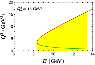
Figure 1: Criteria for selecting the electron beam energy $E$, where the red (green) curve denotes the $E$-$Q^{2}_{\max(\min)}$ relation given by Eq. (23), and the blue line represents the condition $Q^{2}\leq 16\,\text{GeV}^{2}$ required by our theoretical framework. The yellow range indicates the eligible $E$.

Let us now turn to the kinematics of the scattering process $e^{-}p\to\Lambda_{c}\tau^{-}$, in which the $q^{2}$ is bounded by [21]

$$\frac{\alpha-E\sqrt{\lambda}}{m_{p}+2E}\leq q^{2}\leq\frac{\alpha+E\sqrt{\lambda}}{m_{p}+2E}\,,$$ (23)

where

$$\alpha \!\equiv\!E(m_{\Lambda_{c}}^{2}\!-\!m_{p}^{2}\!+\!m^{2}_{\tau}\!-\!2m_{p}E)\!+\!m_{p}m^{2}_{\tau}\,,$$

$$\lambda \!\equiv\!m_{\Lambda_{c}}^{4}\!+\!(m_{p}^{2}\!+\!2m_{p}E\!-\!m^{2}_{\tau})^{2}\!-\!2m_{\Lambda_{c}}^{2}(m_{p}^{2}\!+\!2m_{p}E\!+\!m^{2}_{\tau})\,.$$

Note that the electron mass has been ignored due to $m_{e}/E\ll 1$. The condition of Eq. (23) indicates that the electron beam energy $E$ determines the maximal and minimal values of $Q^{2}$ ($Q^{2}=-q^{2}$), which, in turn, implies that any constraints on $Q^{2}_{\max}$ and $Q^{2}_{\min}$ restrict the $E$ selection. For instance, condition $Q^{2}_{\max}=Q^{2}_{\min}$ indicates a minimal requirement for $E$ ($E\gtrsim 8.33$ GeV); this can also be visualized in Fig. 1 by noting the intersection point of the red and green curves that represent the $E$-$Q^{2}_{\max}$ and $E$-$Q^{2}_{\min}$ relations, respectively. Besides these constraints, we also consider the one from our theoretical framework. Since our analyses are carried out in the framework of $\mathcal{L}_{\text{eff}}$ given by Eq. (1), to ensure the validity of our results, we require $Q^{2}_{\max}$ to not exceed $Q^{2}_{b}=16\,\text{GeV}^{2}\approx m_{b}^{2}$. Such a requirement, depicted by the blue line in Fig. 1, results in an upper bound $E\lesssim 13.41\,\text{GeV}$, provided that the observables one is interested in, such as the total cross section, involve $Q^{2}_{\max}$. Otherwise, $E$ is not bounded from above, since one can always focus on the lower $Q^{2}$ range, even though a high $Q^{2}_{\max}$ is available due to a high $E$.

III Phenomenology analyses

III.1 Observable analyses

The factor $C$ in Eq. (II.2) is connected to the unpolarized differential cross section $d\sigma_{s}$ of the scattering process $e^{-}p\to\Lambda_{c}\tau^{-}$ (cf. Eq. (6)) through the following relation

$$2C=|\mathcal{M}|^{2}=\frac{1}{v^{4}}\sum g_{\alpha}g^{*}_{\beta}\leavevmode\nobreak\ \mathcal{A}_{\alpha-\beta}\,,$$ (24)

where $|\mathcal{M}|^{2}$ is the amplitude squared without spin average of the initial particles, and $\mathcal{A}_{\alpha-\beta}$ with a subscript, e.g., $V_{LL}\!-\!V_{LR}$, represents the reduced amplitude squared that is induced by the interference between the operators $\mathcal{O}^{LL}_{V}$ and $\mathcal{O}^{LR}_{V}$. Since all of the operators in Table 1 can contribute to the scattering process, $g_{\alpha}$ and $g^{*}_{\beta}$ go through all the WCs.

Table 2: Non-zero reduced amplitude squared $\mathcal{A}_{\alpha-\beta}$ that contributes to the cross section of the scattering process $e^{-}p\to\Lambda_{c}\tau^{-}$. The subscript $\alpha-\beta$, e.g., $V_{LL}\!-\!V_{LR}$, indicates $\mathcal{A}_{V_{LL}\!-\!V_{LR}}$ is induced by the interference between the operators $\mathcal{O}^{LL}_{V}$ and $\mathcal{O}^{LR}_{V}$.

	$(g^{LL}_{V})^{*}$	$(g^{LR}_{V})^{*}$	$(g^{LL}_{S})^{*}$	$(g^{LR}_{S})^{*}$	$(g^{LL}_{T})^{*}$
$g^{LL}_{V}$	$\mathcal{A}_{V_{LL}\!-\!V_{LL}}$	$\mathcal{A}_{V_{LL}\!-\!V_{LR}}$	$\mathcal{A}_{V_{LL}\!-\!S_{LL}}$	$\mathcal{A}_{V_{LL}\!-\!S_{LR}}$	$\mathcal{A}_{V_{LL}\!-\!T_{LL}}$
$g^{LR}_{V}$	$\mathcal{A}_{V_{LL}\!-\!V_{LR}}$	$\mathcal{A}_{V_{LR}\!-\!V_{LR}}$	$\mathcal{A}_{V_{LL}\!-\!S_{LR}}$	$\mathcal{A}_{V_{LL}\!-\!S_{LL}}$	$\mathcal{A}_{V_{LR}\!-\!T_{LL}}$
$g^{LL}_{S}$	$\mathcal{A}_{V_{LL}\!-\!S_{LL}}$	$\mathcal{A}_{V_{LL}\!-\!S_{LR}}$	$\mathcal{A}_{S_{LL}\!-\!S_{LL}}$	$\mathcal{A}_{S_{LL}\!-\!S_{LR}}$	$\mathcal{A}_{S_{LL}\!-\!T_{LL}}$
$g^{LR}_{S}$	$\mathcal{A}_{V_{LL}\!-\!S_{LR}}$	$\mathcal{A}_{V_{LL}\!-\!S_{LL}}$	$\mathcal{A}_{S_{LL}\!-\!S_{LR}}$	$\mathcal{A}_{S_{LL}\!-\!S_{LL}}$	$\mathcal{A}_{S_{LR}\!-\!T_{LL}}$
$g^{LL}_{T}$	$\mathcal{A}_{V_{LL}\!-\!T_{LL}}$	$\mathcal{A}_{V_{LR}\!-\!T_{LL}}$	$\mathcal{A}_{S_{LL}\!-\!T_{LL}}$	$\mathcal{A}_{S_{LR}\!-\!T_{LL}}$	$\mathcal{A}_{T_{LL}\!-\!T_{LL}}$
	$(g^{RR}_{V})^{*}$	$(g^{RL}_{V})^{*}$	$(g^{RR}_{S})^{*}$	$(g^{RL}_{S})^{*}$	$(g^{RR}_{T})^{*}$
$g^{RR}_{V}$	$\mathcal{A}_{V_{LL}\!-\!V_{LL}}$	$\mathcal{A}_{V_{LL}\!-\!V_{LR}}$	$\mathcal{A}_{V_{LL}\!-\!S_{LL}}$	$\mathcal{A}_{V_{LL}\!-\!S_{LR}}$	$\mathcal{A}_{V_{LL}\!-\!T_{LL}}$
$g^{RL}_{V}$	$\mathcal{A}_{V_{LL}\!-\!V_{LR}}$	$\mathcal{A}_{V_{LR}\!-\!V_{LR}}$	$\mathcal{A}_{V_{LL}\!-\!S_{LR}}$	$\mathcal{A}_{V_{LL}\!-\!S_{LL}}$	$\mathcal{A}_{V_{LR}\!-\!T_{LL}}$
$g^{RR}_{S}$	$\mathcal{A}_{V_{LL}\!-\!S_{LL}}$	$\mathcal{A}_{V_{LL}\!-\!S_{LR}}$	$\mathcal{A}_{S_{LL}\!-\!S_{LL}}$	$\mathcal{A}_{S_{LL}\!-\!S_{LR}}$	$\mathcal{A}_{S_{LL}\!-\!T_{LL}}$
$g^{RL}_{S}$	$\mathcal{A}_{V_{LL}\!-\!S_{LR}}$	$\mathcal{A}_{V_{LL}\!-\!S_{LL}}$	$\mathcal{A}_{S_{LL}\!-\!S_{LR}}$	$\mathcal{A}_{S_{LL}\!-\!S_{LL}}$	$\mathcal{A}_{S_{LR}\!-\!T_{LL}}$
$g^{RR}_{T}$	$\mathcal{A}_{V_{LL}\!-\!T_{LL}}$	$\mathcal{A}_{V_{LR}\!-\!T_{LL}}$	$\mathcal{A}_{S_{LL}\!-\!T_{LL}}$	$\mathcal{A}_{S_{LR}\!-\!T_{LL}}$	$\mathcal{A}_{T_{LL}\!-\!T_{LL}}$

We list in Table 2 all the non-zero $\mathcal{A}_{\alpha-\beta}$. Already, some patterns emerge. First, $\mathcal{A}_{\alpha-\beta}$ vanishes if induced by interference between two operators with their lepton currents of opposite chiral properties, equivalently $L^{L}_{\alpha}(\lambda)L^{R*}_{\beta}(\lambda)=0$, because the electron mass has been ignored due to $m_{e}/E\ll 1$. Second, all of the $\mathcal{A}$ are real, leading to $\mathcal{A}_{\alpha-\beta}=\mathcal{A}_{\beta-\alpha}$. Third, $\mathcal{A}_{S_{LL}\!-\!S_{LL}}$ is equal to $\mathcal{A}_{S_{LR}\!-\!S_{LR}}$. Finally, simultaneously flipping the chiral properties of the lepton and quark currents of two operators $\mathcal{O}_{\alpha}$ and $\mathcal{O}_{\beta}$ yields the same reduced amplitude squared $\mathcal{A}_{\alpha-\beta}$, e.g., $\mathcal{A}_{V_{RR}\!-\!V_{RL}}=\mathcal{A}_{V_{LL}\!-\!V_{LR}}$. The latter two patterns arise due to the chiral structures of the lepton and quark currents and the form-factor paramertrization of the hadronic matrix elements. Based on these patterns, we only present one $\mathcal{A}_{\alpha-\beta}$ in Table 2, if its duplicates appear.

Table 3: Non-zero reduced amplitude squared $\mathcal{A}^{\tau}_{\alpha-\beta}$ that contains the polarization information of the lepton $\tau$. Note that it has the same subscript with the $\mathcal{A}_{\alpha-\beta}$.

	$(g^{LL}_{V})^{*}$	$(g^{LR}_{V})^{*}$	$(g^{LL}_{S})^{*}$	$(g^{LR}_{S})^{*}$	$(g^{LL}_{T})^{*}$
$g^{LL}_{V}$	$\mathcal{A}^{\tau}_{V_{LL}\!-\!V_{LL}}$	$\mathcal{A}^{\tau}_{V_{LL}\!-\!V_{LR}}$	$\mathcal{A}^{\tau}_{V_{LL}\!-\!S_{LL}}$	$\mathcal{A}^{\tau}_{V_{LL}\!-\!S_{LR}}$	$\mathcal{A}^{\tau}_{V_{LL}\!-\!T_{LL}}$
$g^{LR}_{V}$	$\mathcal{A}^{\tau}_{V_{LL}\!-\!V_{LR}}$	$\mathcal{A}^{\tau}_{V_{LR}\!-\!V_{LR}}$	$\mathcal{A}^{\tau}_{V_{LL}\!-\!S_{LR}}$	$\mathcal{A}^{\tau}_{V_{LL}\!-\!S_{LL}}$	$\mathcal{A}^{\tau}_{V_{LR}\!-\!T_{LL}}$
$g^{LL}_{S}$	$\mathcal{A}^{\tau*}_{V_{LL}\!-\!S_{LL}}$	$\mathcal{A}^{\tau*}_{V_{LL}\!-\!S_{LR}}$	$\mathcal{A}^{\tau}_{S_{LL}\!-\!S_{LL}}$	$\mathcal{A}^{\tau}_{S_{LL}\!-\!S_{LR}}$	$\mathcal{A}^{\tau}_{S_{LL}\!-\!T_{LL}}$
$g^{LR}_{S}$	$\mathcal{A}^{\tau*}_{V_{LL}\!-\!S_{LR}}$	$\mathcal{A}^{\tau*}_{V_{LL}\!-\!S_{LL}}$	$\mathcal{A}^{\tau}_{S_{LL}\!-\!S_{LR}}$	$\mathcal{A}^{\tau}_{S_{LL}\!-\!S_{LL}}$	$\mathcal{A}^{\tau}_{S_{LR}\!-\!T_{LL}}$
$g^{LL}_{T}$	$\mathcal{A}^{\tau*}_{V_{LL}\!-\!T_{LL}}$	$\mathcal{A}^{\tau*}_{V_{LR}\!-\!T_{LL}}$	$\mathcal{A}^{\tau*}_{S_{LL}\!-\!T_{LL}}$	$\mathcal{A}^{\tau*}_{S_{LR}\!-\!T_{LL}}$	$\mathcal{A}^{\tau}_{T_{LL}\!-\!T_{LL}}$
	$(g^{RR}_{V})^{*}$	$(g^{RL}_{V})^{*}$	$(g^{RR}_{S})^{*}$	$(g^{RL}_{S})^{*}$	$(g^{RR}_{T})^{*}$
$g^{RR}_{V}$	$-\mathcal{A}^{\tau}_{V_{LL}\!-\!V_{LL}}$	$-\mathcal{A}^{\tau}_{V_{LL}\!-\!V_{LR}}$	$-\mathcal{A}^{\tau*}_{V_{LL}\!-\!S_{LL}}$	$-\mathcal{A}^{\tau*}_{V_{LL}\!-\!S_{LR}}$	$-\mathcal{A}^{\tau*}_{V_{LL}\!-\!T_{LL}}$
$g^{RL}_{V}$	$-\mathcal{A}^{\tau}_{V_{LL}\!-\!V_{LR}}$	$-\mathcal{A}^{\tau}_{V_{LR}\!-\!V_{LR}}$	$-\mathcal{A}^{\tau*}_{V_{LL}\!-\!S_{LR}}$	$-\mathcal{A}^{\tau*}_{V_{LL}\!-\!S_{LL}}$	$-\mathcal{A}^{\tau*}_{V_{LR}\!-\!T_{LL}}$
$g^{RR}_{S}$	$-\mathcal{A}^{\tau}_{V_{LL}\!-\!S_{LL}}$	$-\mathcal{A}^{\tau}_{V_{LL}\!-\!S_{LR}}$	$-\mathcal{A}^{\tau}_{S_{LL}\!-\!S_{LL}}$	$-\mathcal{A}^{\tau}_{S_{LL}\!-\!S_{LR}}$	$-\mathcal{A}^{\tau*}_{S_{LL}\!-\!T_{LL}}$
$g^{RL}_{S}$	$-\mathcal{A}^{\tau}_{V_{LL}\!-\!S_{LR}}$	$-\mathcal{A}^{\tau}_{V_{LL}\!-\!S_{LL}}$	$-\mathcal{A}^{\tau}_{S_{LL}\!-\!S_{LR}}$	$-\mathcal{A}^{\tau}_{S_{LL}\!-\!S_{LL}}$	$-\mathcal{A}^{\tau*}_{S_{LR}\!-\!T_{LL}}$
$g^{RR}_{T}$	$-\mathcal{A}^{\tau}_{V_{LL}\!-\!T_{LL}}$	$-\mathcal{A}^{\tau}_{V_{LR}\!-\!T_{LL}}$	$-\mathcal{A}^{\tau}_{S_{LL}\!-\!T_{LL}}$	$-\mathcal{A}^{\tau}_{S_{LR}\!-\!T_{LL}}$	$-\mathcal{A}^{\tau}_{T_{LL}\!-\!T_{LL}}$

Similar to $C$, $\Sigma^{a}_{P}$ can be written as

$$2\Sigma^{a}_{P}=\frac{1}{v^{4}}\sum g_{\alpha}g^{*}_{\beta}\leavevmode\nobreak\ \mathcal{A}^{\tau}_{\alpha-\beta}\,,$$ (25)

where the reduced amplitude squared $\mathcal{A}^{\tau}_{\alpha-\beta}$ contains the polarization information of the $\tau$, and shares the same subscript with the $\mathcal{A}_{\alpha-\beta}$. We list in Table 3 all the non-zero $\mathcal{A}^{\tau}_{\alpha-\beta}$. One can see that certain patterns emerging from the $\mathcal{A}_{\alpha-\beta}$ in Table 2 can apply to $\mathcal{A}^{\tau}_{\alpha-\beta}$, too. For instance, $\mathcal{A}^{\tau}_{\alpha-\beta}$ also vanishes if induced by interference between two operators with their lepton currents of opposite chiral properties, equivalently $L^{L}_{\alpha}(\lambda)L^{R*}_{\beta}(\lambda^{\prime})=0$, due to the same reason. Another example is that the relation $\mathcal{A}^{\tau}_{S_{LL}\!-\!S_{LL}}\!=\!\mathcal{A}^{\tau}_{S_{LR}\!-\!S_{LR}}$ also holds in this case.

Of course, distinct differences exist between the two cases. First, instead of $\mathcal{A}^{\tau}_{\alpha-\beta}\!=\!\mathcal{A}^{\tau}_{\beta-\alpha}$, $\mathcal{A}^{\tau}_{\alpha-\beta}\!=\!\mathcal{A}^{\tau*}_{\beta-\alpha}$ in general for $\alpha\neq\beta$ (one exception is when both the $\alpha$ and $\beta$ denote the vector operators). Such a difference arises from the appearance of $\varepsilon_{\{k\}\{k^{\prime}\}\{s_{a}\}\{p\}}$, which is always accompanied by the imaginary unit $i$. Interestingly enough, the very same term generates a non-zero $P_{P}$ provided that all the WCs are complex. For $\alpha=\beta$, on the other hand, $\mathcal{A}^{\tau}_{\alpha-\alpha}$ remains real due to missing the $\varepsilon_{\{k\}\{k^{\prime}\}\{s_{a}\}\{p\}}$. Based on these arguments, one can see that $P_{P}$ vanishes in a pure-vector scenario, i.e., only the vector operators $\mathcal{O}_{V}$ are activated. And it also vanishes if only one WC is turned on in the $\mathcal{L}_{\text{eff}}$, i.e., all other WCs are set to zero. The second difference is that, contrary to the $\mathcal{A}_{\alpha-\beta}$ case, simultaneously flipping the chiral properties of the lepton and quark currents of two operators $\mathcal{O}_{\alpha}$ and $\mathcal{O}_{\beta}$ now yields $-\mathcal{A}^{\tau}_{\alpha-\beta}$, e.g., $\mathcal{A}^{\tau}_{V_{RR}\!-\!V_{RL}}=-\mathcal{A}^{\tau}_{V_{LL}\!-\!V_{LR}}$.

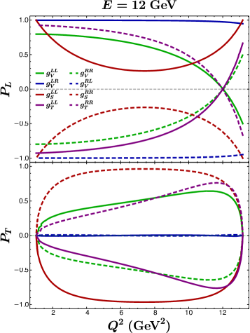
Figure 2: Variations of the polarization $P_{L}$ and $P_{T}$ with respect to $Q^{2}$ in different NP scenarios, where we have set the electron beam energy at $E=12$ GeV.

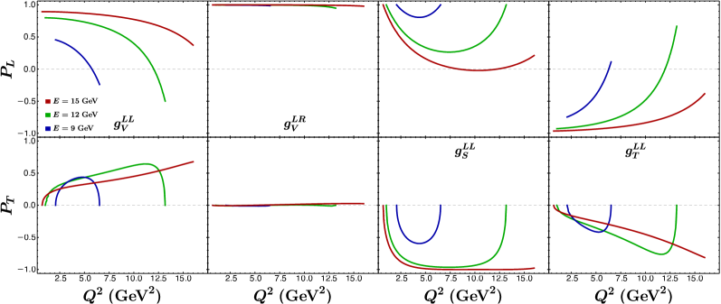
Figure 3: The polarization $P_{L,T}$ in various NP scenarios with three different electron beam energies. Note that the NP scenarios with right-handed lepton current are not presented and neither is the NP $g^{LR}_{S}$. Also only the $P_{L,T}$ within the kinematic range $Q^{2}\in[Q^{2}_{\text{min}},16\ \text{GeV}^{2}]$ are presented for $E=$15 GeV.

With $C$ and $\Sigma^{a}_{P}$ given respectively in Eqs. (24) and (25), the polarization components $P_{a}$ are now formulated in terms of the $\mathcal{A}_{\alpha-\beta}$ and $\mathcal{A}^{\tau}_{\alpha-\beta}$ as well as the WCs. Since the WCs have not been determined yet, it will be difficult to explore the behavior of $P_{a}$ in general with respect to the kinematics $Q^{2}$, the beam energy $E$, etc. However, if only one operator $\mathcal{O}_{\alpha}$ in Eq. (1) is activated at a time, the $P_{a}$ become independent of the WC $g_{\alpha}$. Immediately, $P_{P}$ in these NP scenarios vanishes, as indicated by the patterns arising in Tables 2 and 3. In addition, $P_{L,T}$ in the NPs $g^{LL}_{V}$ and $g^{RR}_{V}$ differ only by a minus sign; the same conclusion also holds for the NP pairs ($g^{LR}_{V}$, $g^{RL}_{V}$), ($g^{LL}_{S}$, $g^{RR}_{S}$), ($g^{LR}_{S}$, $g^{RL}_{S}$), and ($g^{LL}_{T}$, $g^{RR}_{T}$). Besides the simple case above, the $P_{a}$ can also be independent of the WCs, if only $\mathcal{O}^{LL}_{S}$ and $\mathcal{O}^{LR}_{S}$ ($\mathcal{O}^{RR}_{S}$ and $\mathcal{O}^{RL}_{S}$) are activated simultaneously. To justify this one can check the explicit expressions of the corresponding $\mathcal{A}_{\alpha-\beta}$ and $\mathcal{A}^{\tau}_{\alpha-\beta}$ in Appendixes B and C.

The behavior of $P_{a}$ predicted above in the two simple cases can also be justified graphically. Let us focus on the first one and explore in Fig. 2 how the $P_{L,T}$ vary with respect to the $Q^{2}$ in various NP scenarios (note $P_{P}=0$). For a simple demonstration, we consider the beam energy $E=12$ GeV as a benchmark. And since the $P_{L,T}$ induced by the $\mathcal{O}^{LL}_{S}$ and $\mathcal{O}^{LR}_{S}$ ($\mathcal{O}^{RR}_{S}$ and $\mathcal{O}^{RL}_{S}$) are identical, only the former are presented, as already argued in the second simple case. Now one can clearly see that the sign of $P_{L,T}$ indeed flips as one simultaneously flips the chiral properties of the lepton and quark currents of an operator—check the solid and dashed curves in the same color. In addition, the lepton $\tau$ produced in the NP $g_{V}^{LR}$ ($g_{V}^{RL}$) is almost fully polarized along the longitudinal direction, as indicated by the blue (dashed) curves. In the NP $g_{S}^{LL}$ ($g_{S}^{RR}$) denoted by the red (dashed) curves, on the other hand, the $\tau$ is fully polarized in the longitudinal direction only at the maximal and minimal $Q^{2}$; in the middle $Q^{2}$ regions, say $Q^{2}\in(5,9)$ GeV², it prefers being polarized transversely. Finally, the $P_{L,T}$ in the NPs $g_{V}^{LL}$ and $g_{T}^{LL}$ ($g_{V}^{RR}$ and $g_{T}^{RR}$) display a roughly opposite pattern and, interestingly, the $P_{L}$ in both scenarios becomes zero at $Q^{2}\simeq 12$ GeV².

Finally, we explore the dependence of $P_{L,T}$ on the electron beam energy $E$. Based on the observations made in Fig. 2, we shall focus on the NPs $g_{V}^{LL}$, $g_{V}^{LR}$, $g_{S}^{LL}$, and $g_{T}^{LL}$. As shown in Fig. 3, the $P_{L}$ ($P_{T}$) in the NP $g_{V}^{LR}$ remains $+1$ (0) to a very good approximation in the whole allowed $Q^{2}$ regions. Meanwhile, the $P_{L}$ ($P_{T}$) in the NP $g_{S}^{LL}$ at the corresponding $Q^{2}_{\text{min}}$ and $Q^{2}_{\text{max}}$ remains $+1$ (0) for $E=9,12$ GeV; this pattern would also apply to the case of $E=15$ GeV if its corresponding $Q^{2}_{\text{max}}$ were not excluded by our theoretical framework. On the other hand, the $P_{T}$ in the middle $Q^{2}$ regions becomes more favorite than the $P_{L}$ for the $\tau$ as $E$ increases (note $P_{L}=0$ and $P_{T}=-1$ at $Q^{2}\simeq 7.5,12.5$ GeV² for $E=15$ GeV). As for the NPs $g_{V}^{LL}$ and $g_{T}^{LL}$, both the minimal and maximal values of the $P_{L}$ and the minimum of the $P_{T}$ change vastly as $E$ increases, but the roughly opposite pattern between the two NP cases remains.

III.2 NP model identification

We considered in Ref. [54] the low-energy polarized scattering process $e^{-}p\to e^{-}\Lambda_{c}$, and demonstrated in a model-independent way that 15 NP scenarios constructed only with the vector operators $\mathcal{O}_{V}$ can be effectively disentangled from each other by measuring 4 spin asymmetries $A^{e}_{L}$, $A^{p}_{L}$, $A^{ep}_{L3}$, and $A^{ep}_{L6}$. The key ingredients are the longitudinal polarized electron beam and proton target. In this subsection, we will also define 15 NP scenarios in a similar way, and show that they can be distinguished from each other by using the longitudinal polarized electron beam and by measuring the $P_{T}$ of the $\tau$.

Table 4: The $P_{T}$ predicated in the cases I-XV with the electron beam left- ($e_{L}$) and right-handed ($e_{R}$) polarized, where $c$ is expected to be away from 0 and 0.5 in general; see text for details.

	I	II	III	IV	V
$P_{T}$($e_{L}$)	0.5	0	0	0	$c$
$P_{T}$($e_{R}$)	0	0	0	$-0.5$	0
	VI	VII	VIII	IX	X
$P_{T}$($e_{L}$)	0.5	0.5	0	0	0
$P_{T}$($e_{R}$)	0	$-0.5$	0	$-0.5$	$-c$
	XI	XII	XIII	XIV	XV
$P_{T}$($e_{L}$)	$c$	$c$	0.5	0	$c$
$P_{T}$($e_{R}$)	0	$-0.5$	$-c$	$-c$	$-c$

To begin with, let us introduce the new 15 NP scenarios, which are constructed with the 4 vector operators $\mathcal{O}_{V}^{LL}$, $\mathcal{O}_{V}^{LR}$, $\mathcal{O}_{V}^{RL}$, and $\mathcal{O}_{V}^{RR}$, as well as their possible combinations:

1. cases with one vector operator: (I) $\mathcal{O}_{V}^{LL}$, (II) $\mathcal{O}_{V}^{LR}$, (III) $\mathcal{O}_{V}^{RL}$, and (IV) $\mathcal{O}_{V}^{RR}$;

2. cases with two vector operators: (V) $\mathcal{O}_{V}^{LL}$ and $\mathcal{O}_{V}^{LR}$, (VI) $\mathcal{O}_{V}^{LL}$ and $\mathcal{O}_{V}^{RL}$, (VII) $\mathcal{O}_{V}^{LL}$ and $\mathcal{O}_{V}^{RR}$, (VIII) $\mathcal{O}_{V}^{LR}$ and $\mathcal{O}_{V}^{RL}$, (IX) $\mathcal{O}_{V}^{LR}$ and $\mathcal{O}_{V}^{RR}$, and (X) $\mathcal{O}_{V}^{RL}$ and $\mathcal{O}_{V}^{RR}$;

3. cases with three vector operators: (XI) $\mathcal{O}_{V}^{LL}$, $\mathcal{O}_{V}^{LR}$, and $\mathcal{O}_{V}^{RL}$, (XII) $\mathcal{O}_{V}^{LL}$, $\mathcal{O}_{V}^{LR}$, and $\mathcal{O}_{V}^{RR}$, (XIII) $\mathcal{O}_{V}^{LL}$, $\mathcal{O}_{V}^{RL}$, and $\mathcal{O}_{V}^{RR}$, and (XIV) $\mathcal{O}_{V}^{LR}$, $\mathcal{O}_{V}^{RL}$, and $\mathcal{O}_{V}^{RR}$;

4. cases with four vector operators: (XV) $\mathcal{O}_{V}^{LL}$, $\mathcal{O}_{V}^{LR}$, $\mathcal{O}_{V}^{RL}$, and $\mathcal{O}_{V}^{RR}$.

And we assume no scalar and tensor operators are activated.

For a simple demonstration, we once again consider the benchmark beam energy $E=12$ GeV. Supposing the scattering experiment is run twice with the electron beam left- ($e_{L}$) and right-handed ($e_{R}$) polarized accordingly, we collect the complete results for the cases I–XV in Table 4. And for the sake of simplicity, we focus on $Q^{2}\simeq 6$ GeV², so that $P_{T}\simeq 0.5\,(0)$ for the NP scenario $g^{LL}_{V}$ ($g^{LR}_{V}$), as shown in Fig. 2. The constant $c$, depending on $|g_{V}^{LL}|^{2}$, $|g_{V}^{LR}|^{2}$, and $\text{Re}[g_{V}^{LL}g_{V}^{LR*}]$, is expected to be away from 0 and 0.5 in general. Now based on their results of $P_{T}$ with $e_{L}$ and $e_{R}$, those NP scenarios can be divided into nine groups: {II, III, VIII}, {I, VI}, {V, XI}, {IV, IX}, {X, XIV}, {VII}, {XII}, {XIII}, and {XV}. Already, the 4 NP scenarios listed accordingly in the last 4 groups can be distinguished from each other and the rest of the NP models. To further disentangle the remaining 11 cases, one can simply check the events of the scattering process for the two experiments. Take the first group {II, III, VIII} for an illustration. If one observes events with the $e_{L}$ beam, while none with the $e_{R}$ beam, the NP scenario is the case II; if the observation is completely opposite, it belongs to the case III; if one observe events in both times, it shall be the case VIII. In this way, the NP scenarios II, III, and VIII are disentangled. Following the same procedure, one can also disentangle the rest 8 cases.

Let us conclude this subsection by making the following comment. In Ref. [54], seven LQ models $S_{1}$, $R_{2}$, $S_{3}$, $U_{3}$, $\tilde{V}_{2}$, $\tilde{U}_{1}$ and $V_{2}$ were disentangled by using the polarized scattering process $e^{-}p\to e^{-}\Lambda_{c}$; additional processes are needed to further distinguish $S_{3}$ from $U_{3}$, since they yield the same effective operator $\mathcal{O}_{V}^{LL}$. To achieve this goal, the scalar and tensor contributions in the LQ models $S_{1}$ and $R_{2}$ were ignored, which was a reasonable assumption, since the WCs of the scalar and tensor operators are closed related in the two LQ models and the former are stringently constrained by the leptonic $D$-meson decays [21, 65]. For the WCs of the $\mathcal{L}_{\text{eff}}$ in Eq. (1), on the other hand, none of them has been constrained more stringently than the others, as to be shown in Sec. IV. Thus it will be more involved to fully disentangle the LQ models. Nonetheless, the LQ models $U_{3}$ ($S_{3}$), $\tilde{V}_{2}$, $\tilde{U}_{1}$ and $V_{2}$ are already distinguished through the identification mechanism, since they correspond to the cases I, II, IV, and III, respectively. Moreover, the scalar LQ models $S_{1}$ and $R_{2}$ can be disentangled from the others, because they generate a non-zero $P_{P}$—induced by the interference among the vector, scalar, and tensor operators—whereas the others do not.

III.3 Impacts from the form factors

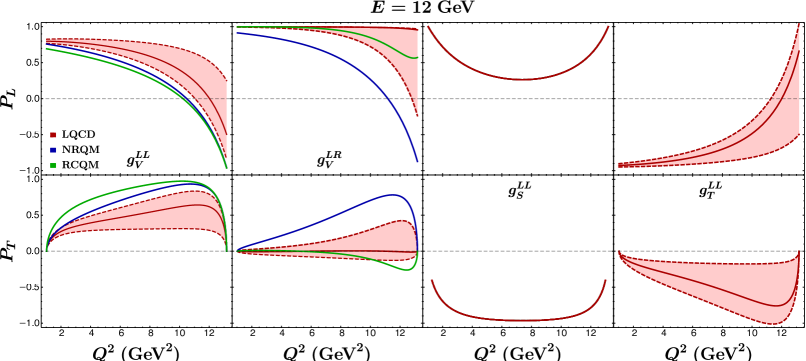
Figure 4: The polarization $P_{L,T}$ as a function of $Q^{2}$, predicted with the form factors calculated in LQCD (red), NRQM (blue), and RCQM (green), respectively. Note that the 1$\sigma$-level statistical uncertainties of the form factors in LQCD have been propagated to all the observables, as denoted by the outer red regions. In addition, the $P_{L,T}$ denoted by the three colors overlap perfectly for the NP $g^{LL}_{S}$, while for the NP $g^{LL}_{T}$ only the LQCD results are presented.

As mentioned in Sec. II.4, the primary results of the form factors we adopt are from the LQCD calculations, since they provide us with an error estimation [56]. Yet our calculation has only involved the central values of these inputs so far. Given that the uncertainties of the form factors can affect the theoretical predictions significantly [53, 33], they should be taken into account in the analyses of this work, too. In addition, the ambiguity arising in extrapolating the form factors to positive $q^{2}$ with different parametrization schemes can have a huge impact on theoretical predictions [64, 53, 33]; this impact can even dwarf the one induced by the error propagation of the form-factor uncertainties. Since our analysis is based on the same extrapolation, we should also examine if the same observation applies to the $P_{a}$ in various NP scenarios in this work.

As a simple illustration, let us focus again on the first simple case, i.e., only one WC is activated at a time. We evaluate in Fig. 4 the $P_{L,T}$ with the form factors calculated in LQCD (red), NRQM (blue), and RCQM (green), respectively. And we also take account of the $1\sigma$-level statistical uncertainties of the form factors in the LQCD case. Following the same argument made in Fig. 2, we only present the NP scenarios $g_{V}^{LL}$, $g_{V}^{LR}$, $g_{S}^{LL}$, and $g_{T}^{LL}$ in this figure. It can be seen that in the case of $g_{V}^{LL}$, the LQCD always predicts the largest $P_{L}$ but the smallest $P_{T}$, whereas the situation is completely opposite in the RCQM. For the NP $g_{V}^{LR}$, on the other hand, the RCQM predicts compatible $P_{L,T}$ with the LQCD at the $1\sigma$ level, while the NRQM produces the smallest $P_{L}$ but the largest $P_{T}$. Contrary to the two NP scenarios above, situation in the NP $g^{LL}_{S}$ is much simpler. Since both the $P_{L}$ and $P_{T}$ are independent of the WC $g^{LL}_{S}$, all of the three models generate the same $P_{L,T}$; for details of the $P_{L,T}$ in this case we refer the reader to Appendix C. Finally, for the NP $g^{LL}_{T}$, only the LQCD results are presented, since the relevant form factors have not been calculated in other two models.

Despite the complicated behaviors of the $P_{L,T}$ calculated with various form-factor parametrization schemes in the NP scenarios, two overall observations can be made easily. The first one is that the uncertainties of the $P_{L,T}$ from the error propagation of the statistical uncertainties of the form factors in the LQCD increase along with the $Q^{2}$—these uncertainties of the $P_{L,T}$ would become even larger if the systematical ones were taken into account, too. Such a pattern is closely related to the behaviors of the form factors with respect to the $Q^{2}$ [33]. The other observation is that the uncertainties of the $P_{L,T}$ due to the different schemes overwhelm the ones induced by the error propagation of the form-factor uncertainties. Clearly, these two observations are consist with the results of Ref. [33].

The uncertainties of the $P_{L,T}$ will certainly affect the model identification in Sec. III.2. We have shown that a distinct difference between the predicted $P_{T}$ in the NPs $g^{LL}_{V}$ and $g^{LR}_{V}$ at a certain $Q^{2}$ is one of the key ingredients in the success of NP model identification. Clearly, such a difference will be blurred when the uncertainties discussed above are taken into account, as shown in Fig. 4. We note that the largest possible $P_{T}$ in the NP $g^{LR}_{V}$ (denoted by the blue curve) exceeds the smallest one in the NP $g^{LL}_{V}$ (denoted by the lower, red dashed curve) at $Q^{2}\simeq 5$ GeV², indicating that the identification mechanism will fail in the $Q^{2}>5$ GeV² regions. Even if one focuses only on the LQCD results, the mechanism will also fail at $Q^{2}\geq 10$ GeV², since the largest possible $P_{T}$ in the NP $g^{LR}_{V}$ (denoted by the upper, red dashed curve) exceeds the smallest one in the NP $g^{LL}_{V}$ (denoted by the lower, red dashed curve) in this regions. The situation will certainly becomes even tougher for this mechanism if the systematical uncertainties of the form factors are considered, too.

IV Prospect and constraints

We now evaluate the prospect for observing the process $e^{-}p\to\Lambda_{c}\tau^{-}(\to\pi^{-}\nu_{\tau},\rho^{-}\nu_{\tau},\ell^{-}\bar{\nu}_{\ell}\nu_{\tau})$ in the framework of the $\mathcal{L}_{\text{eff}}$. As mentioned in Sec. II.2, this cascade process can be broken down into the QE scattering $e^{-}p\to\Lambda_{c}\tau^{-}$ and the successive decays $\tau^{-}\to\pi^{-}\nu_{\tau},\rho^{-}\nu_{\tau},\ell^{-}\bar{\nu}_{\ell}\nu_{\tau}$. Given that the former is a cLFV process, the cascade process would certainly suffer from low experimental statistics. To alleviate this problem, we consider all the successive decays of the lepton $\tau$ in this process and integrate over all the variables in Eq. (II.3); in other words, we shall consider the total cross section.

We propose searching for the cascade process through a fixed-target experiment, whose event rate is given by

$$\frac{dN}{dt}\!=\!\mathcal{L}\sigma\,.$$ (26)

The luminosity $\mathcal{L}$ reads $\mathcal{L}=IL\rho_{T}$, with $I$ being the beam intensity, and $L$ and $\rho_{T}$ denoting the length and the number density of the proton target, respectively. The total cross section $\sigma$ is related to the $\sigma_{s}$, the unpolarized one of the QE scattering process, through the relation $\sigma=\sum_{d}\mathcal{B}_{d}\sigma_{s}$, as indicated by Eq. (22).

From Eq. (26), it is clear that to perform a concrete event-rate estimation for the scattering experiment, we have to choose a suitable experimental setup and assign proper values to the WCs. For the former, we prefer the 12 GeV CEBAF at JLab [27]—specifically, the proposed Solenoidal Large Intensity Device (SoLID) [68], which is feasible to study subthreshold $J/\psi$ production from liquid hydrogen [69] or deuteron [70] (all proton targets). We note that the produced $J/\psi$ is reconstructed through its decay into a lepton pair ($e^{+}e^{-}$) in these experiments [69, 70]. By analogy, we expect (or assume) the produced $\Lambda_{c}$ of the cascade process can also be reconstructed through its decay products and the visible decay products ($\rho,\pi,\ell$) of the $\tau$ can be detected. Thus, we choose the same experimental setup as Ref. [70], i.e., the 12 GeV electron beam with intensity up to 1.25 $\mu$A and the liquid deuteron target, which together make up the overall luminosity $\mathcal{L}=1.2\times 10^{37}$ cm^-2s^-1. With the beam energy $E=12$ GeV, the $\sigma$ can be now written as

$$\sigma\!=\! \frac{\sum_{d}\mathcal{B}_{d}G_{F}^{2}}{32\pi FEm_{p}}\big{\{}1.86\left(|g_{V}^{LL}|^{2}+|g_{V}^{RR}|^{2}\right)$$

$$+1.20\left(|g_{V}^{LR}|^{2}+|g_{V}^{RL}|^{2}\right)+13.60\left(|g_{T}^{LL}|^{2}+|g_{T}^{RR}|^{2}\right)$$

$$+0.51\left(|g_{S}^{LL}|^{2}+|g_{S}^{RR}|^{2}+|g_{S}^{LR}|^{2}+|g_{S}^{RL}|^{2}\right)$$

$$\!+\!1.01\text{Re}\left[g_{V}^{LL}g_{S}^{LL*}\!+\!g_{V}^{RR}g_{S}^{RR*}\!+\!g_{V}^{LR}g_{S}^{LR*}\!+\!g_{V}^{RL}g_{S}^{RL*}\right]$$

$$\!+\!0.56\text{Re}\left[g_{V}^{LL}g_{S}^{LR*}\!+\!g_{V}^{RR}g_{S}^{RL*}\!+\!g_{V}^{LR}g_{S}^{LL*}\!+\!g_{V}^{RL}g_{S}^{RR*}\right]$$

$$+0.65\text{Re}\left[g_{S}^{LL}g_{S}^{LR*}+g_{S}^{RR}g_{S}^{RL*}\right]$$

$$+0.90\text{Re}\left[g_{V}^{LL}g_{V}^{LR*}+g_{V}^{RR}g_{V}^{RL*}\right]$$

$$-4.39\text{Re}\left[g_{V}^{LL}g_{T}^{LL*}+g_{V}^{RR}g_{T}^{RR*}\right]$$

$$+0.36\text{Re}\left[g_{V}^{LR}g_{T}^{LL*}+g_{V}^{RL}g_{T}^{RR*}\right]$$

$$-1.98\text{Re}\left[g_{S}^{LL}g_{T}^{LL*}+g_{S}^{RR}g_{T}^{RR*}\right]$$

$$+0.38\text{Re}\left[g_{S}^{LR}g_{T}^{LL*}+g_{S}^{RL}g_{T}^{RR*}\right]\big{\}}\!\times\!10^{3}\ \text{GeV}^{6}\,.$$ (27)

For the general expression of the $d\sigma/dq^{2}$, we refer the reader to Appendix B.

We now turn to the values of the WCs. Thus far, available constraints on the WCs are solely set by the analyses of high-$p_{T}$ dilepton invariant mass tails in $pp\to\tau^{\pm}e^{\mp}$ [19]. Taking account of the renormalization group (RG) running effects neglected in Ref. [19], and assuming only one WC contributes to the process at a time, we list in Table 5 the upper bounds at the $90\%$ confidence level (CL). For an optimistic event-rate estimation, we take those upper bounds for the WCs. Note that since $O_{S}^{LR}$ and $O_{S}^{RL}$ were not included in the $\mathcal{L}_{\text{eff}}$ in Ref. [19], no constraints on their WCs $g^{LR}_{S}$ and $g^{RL}_{S}$ has been set yet.

Table 5: Summary of the upper bounds on the WCs $g$ from the high-$p_{T}$ dilepton invariant mass tails (at $90\%$ CL) and the $e^{-}p\to\Lambda_{c}\tau^{-}(\to\pi^{-}\nu_{\tau},\rho^{-}\nu_{\tau},\ell^{-}\bar{\nu}_{\ell}\nu_{\tau})$ scattering processes in the framework of the $\mathcal{L}_{\text{eff}}$ by Eq. (1). Note that a common factor $10^{-3}$ has been factored out, and constraints on $g^{LR}_{S}$ and $g^{RL}_{S}$ have not been set by the high-$p_{T}$ dilepton invariant mass tails [19].

Processes	$\big{|}g^{LL,RR}_{V}\big{|}$	$\big{|}g^{LR,RL}_{V}\big{|}$	$\big{|}g^{LL,RR}_{S}\big{|}$	$\big{|}g^{LL,RR}_{T}\big{|}$
$pp\to\tau^{\pm}e^{\mp}$ [19]	5.27	5.27	11.1	2.11
$e^{-}p\to\Lambda_{c}\tau^{-}(\to d\nu_{\tau})$	1.40	1.74	2.67	0.52

Table 6: Summary of the event-rate estimations for the $e^{-}p\to\Lambda_{c}\tau^{-}(\to\pi^{-}\nu_{\tau},\rho^{-}\nu_{\tau},\ell^{-}\bar{\nu}_{\ell}\nu_{\tau})$ processes in the first simple case discussed in Sec. III.1. Note that we have set $\sum_{d}\mathcal{B}_{d}=70\%$ and assumed no event is observed after 1 year’s running of the experiment. And the event rate is given in units of $N$/yr.

$g^{LL,RR}_{V}$	$g^{LR,RL}_{V}$	$g^{LL,RR}_{S}$	$g^{LL,RR}_{T}$
14.16	9.13	17.22	16.59

Supposing a run time of 1 year (yr) and 100% detecting efficiency of the visible final particles, we evaluate the expected event rates in units of number per year ($N$/yr) for the first simple case discussed in Sec. III.1. The final results are listed in Table 6. It can be seen that comparable event rates can be expected for the NP $g_{V}^{LL,RR}$, $g^{LL,RR}_{S}$, and $g^{LL,RR}_{T}$. Compared with the NP $g_{V}^{LL,RR}$, the predicted event rate for the NP $g_{V}^{LR,RL}$, on the other hand, is slightly smaller, though its WC takes the same value as the $g_{V}^{LL,RR}$. The underlying reason is their different reduced amplitude squared $\mathcal{A}$, as explicitly shown in Eq. (IV) and in Eq. (B) for general cases. In fact, this is an unique character of the QE scattering process mediated by $\ell u\to\ell^{(\prime)}c$ in our framework; one can see that the constraints on the WCs $g_{V}^{LL,RR}$ and $g_{V}^{LR,RL}$ set by the charmed-hadron weak decays and the high-$p_{T}$ dilepton invariant mass tails are always the same (see, e.g., Refs. [21, 54]).

The expected event rates in Table 6, though non-zero, are still not big enough to extract the $P_{a}$ of the $\tau$ with good statistics. One way out is to consider the facilities with higher luminosity. We note that even higher luminosity ($10^{38}$ to $10^{39}$ cm^-2s^-1) can be achieved in Hall C at JLab in the upcoming era [27]. On top of that, both liquid hydrogen and deuterium targets and polarized electron beams are available. If our proposed experiment can be conducted in this hall, not only can the expected event rate be further enhanced, extraction of the $P_{a}$ and NP model identification may become promising, too.

The event rates in Table 6 are what one can expect in the best scenario, because they are carried out with the upper limits of the WCs. Therefore, it is still possible that no event of the cascade process will be observed with our preferred experimental setup in future. If such a worst-case scenario indeed happens, our proposed scattering experiment can still set competitive constraints on the WCs, as shown in Table 5, where we have also assumed a run time of 1 yr and 100% detecting efficiency of the visible final particles. Surely more stringent constraints can be obtained if the experiment can be conducted in the Hall C at JLab in the future.

However, to fully pinpoint the WCs of the $\mathcal{L}_{\text{eff}}$ in Eq. (1), clearly more observables are needed. Recall that we had to make the assumption, i.e., only one WC contributes at a time, to get the constraints listed in Table 5. Even if the purely tauonic $D$-meson decays were measured in the future, they would be still not enough, since they are only sensitive to the axial and pseudo-scalar four-fermion operators of the $\mathcal{L}_{\text{eff}}$. Since the polarization components $P_{a}$ of the $\tau$ involve all the effective operators of the $\mathcal{L}_{\text{eff}}$ (see Appendix C), they can partially fill the gap, though they are more difficult to measure than the cross section, as already indicated in Table 6. One may also consider the QE scattering with both the electron beam and proton target polarized, since polarized QE scattering processes can also shed light on the NP Dirac structures [54].

Finally we would like point out that our predictions in Tables 5 and 6 can be weakened by the non-100% detecting efficiency of the produced particles, such as the $\Lambda_{c}$ baryon, since it may be hard to keep track of all its decay products. Thus a sophisticated detecting system for these particles is crucial. Our results can also be affected significantly by the uncertainties of the form factors. As demonstrated in Sec. III.3, they can exert huge influence on the predictions of $P_{L,T}$, which in turn affect the efficiency of the NP model identification. By analogy, they will certainly have a huge impact on the event-rate estimation and the constraints on the WCs. All this calls for a more concrete form factor parametrization scheme and better control of the uncertainties in future LQCD calculations.

V Conclusion

We have proposed searching for NP through the polarization of the $\tau$ lepton in the QE scattering process $e^{-}p\to\Lambda_{c}\tau^{-}$. As analyzing modes for the $\tau$ polarization, we have considered its four dominant decays $\tau^{-}\to\pi^{-}\nu_{\tau}$, $\tau^{-}\to\rho^{-}\nu_{\tau}$, and $\tau^{-}\to\ell^{-}\bar{\nu}_{\ell}\nu_{\tau}$, and demonstrated that its three polarization components $P_{a}$ can be extracted from the analyses of the kinematics of its visible decay products.

Working in the framework of a general low-energy effective Lagrangian given by Eq. (1), we have first performed a detailed analysis of the $P_{a}$ and discovered some interesting patterns. First, the $P_{a}$ in a NP scenario with only left-handed lepton currents differ by a minus sign to that in another NP scenario with only right-handed lepton currents, as shown in Tables 2 and 3. Second, due to missing the $\varepsilon_{\{k\}\{k^{\prime}\}\{s_{a}\}\{p\}}$, the perpendicular component $P_{P}$ vanishes in the simplest NP scenario, i.e., only one WC is activated at a time, and in the pure-vector case, i.e., only the vector operators $\mathcal{O}_{V}$ are activated. Third, the $P_{a}$ can be independent of the WCs in certain NP scenarios, e.g., when only $\mathcal{O}^{LL}_{S}$ and $\mathcal{O}^{LR}_{S}$ ($\mathcal{O}^{RR}_{S}$ and $\mathcal{O}^{RL}_{S}$) are activated simultaneously. Based on these patterns, we have then shown that 15 NP models constructed with only vector operators can be distinguished from each other by using the longitudinal polarized electron beam and measuring the transverse component $P_{T}$ of the $\tau$. We have also explored the impacts of the form factors in various aspects and observed that large uncertainties of the polarization observables arise from using the different schemes and dwarf that from the error propagation of the form factors, which is consist with our previous result in Ref. [33], though it was focused on the neutrino QE scattering process $\nu_{\tau}n\to\Lambda_{c}\tau^{-}$.

We have finally performed a simple event-rate estimation for the cascade process $e^{-}p\!\to\!\Lambda_{c}\tau^{-}(\!\to\!\pi^{-}\nu_{\tau},\rho^{-}\nu_{\tau},\ell^{-}\bar{\nu}_{\ell}\nu_{\tau})$ in the simplest NP scenarios with our preferred experimental setup and the upper boundary of the WCs from the analyses of high-$P_{T}$ dilepton invariant mass tails. Although promising event rate can be expected for this process, it remains challenging to extract the $P_{a}$ of the $\tau$ with good statistics, which thus calls for an experimental setup with even higher luminosity. Nonetheless, even in the worst-case scenario—no signals is observed at all—we have shown in a model-independent way that the low-energy scattering process can provide competitive constraints, in comparison with the high-$P_{T}$ dilepton invariant mass tails.

Appendix A Calculation of the spin density matrices

A.1 $\tau$ decay density matrix

The helicity amplitude for the $\tau^{-}\to\pi^{-}\nu_{\tau}$ decay is given by

$$\mathcal{M}_{\lambda}(\tau^{-}\to\pi^{-}\nu_{\tau})=i\sqrt{2}G_{F}V^{*}_{ud}f_{\pi}p^{\mu}_{\pi}\bar{u}_{\nu_{\tau}}\gamma_{\mu}P_{L}u_{\tau}(\lambda)\,,$$ (28)

where $f_{\pi}$ is the $\pi$ decay constant and $\lambda=\{1/2,-1/2\}$ characterizes the helicity of the $\tau$. With the amplitude above, we compute the spin density decay matrix of the $\tau$ in this decay process [32],

$$(\rho^{D}_{\pi})_{\lambda\lambda^{\prime}} =\mathcal{M}_{\lambda}\mathcal{M}^{*}_{\lambda^{\prime}}$$

$$=\frac{|G|^{2}}{4}\Big{[}2m^{2}_{\tau}(m^{2}_{\tau}\!-\!m^{2}_{\pi})\delta_{\lambda\lambda^{\prime}}\!-\!4m^{3}_{\tau}(p_{\pi}\cdot s^{a})\sigma^{a}_{\lambda\lambda^{\prime}}\Big{]}\,,$$ (29)

where $G=i\sqrt{2}G_{F}V^{*}_{ud}f_{\pi}$, $\sigma^{a}$ ($a=1,2,3$) are the Pauli matrices, and the subscript $\pi$ in $\rho^{D}_{\pi}$ indicates the $\tau^{-}\to\pi^{-}\nu_{\tau}$ decay channel. The spacelike four-vector $s^{a}_{\mu}$ are the spin vectors of the $\tau$, which together with the $k^{\prime}/m_{\tau}$ form an orthonormal set [32],

$$\frac{k^{\prime}}{m_{\tau}}\cdot s^{a} =0\,,\quad s^{a}\cdot s^{a\prime}=-\delta^{aa^{\prime}}\,,$$

$$\sum_{a}s^{a}_{\mu}\cdot s^{a}_{\nu} =-g_{\mu\nu}+\frac{k^{\prime}_{\mu}k^{\prime}_{\nu}}{m^{2}_{\tau}}\,.$$ (30)

Note that in computing the density matrix $\rho^{D}_{\pi}$ in Eq (A.1), as well as the rest of density matrices for production and decay of the $\tau$, we always employ the Bouchiat-Michel formulae [71, 72, 32]:

$$u_{\lambda^{\prime}}(p)\bar{u}_{\lambda}(p)=\frac{1}{2}\left[\delta_{\lambda\lambda^{\prime}}+\sum_{a}\gamma_{5}\not{s}^{a}\sigma^{a}_{\lambda\lambda^{\prime}}\right](\not{p}+m)\,.$$ (31)

The helicity amplitude for the $\tau^{-}\to\rho^{-}\nu_{\tau}$ decay is written as

$$\mathcal{M}^{\lambda_{\rho}}_{\lambda}(\tau^{-}\!\to\!\rho^{-}\nu_{\tau})\!=\!i\sqrt{2}G_{F}V^{*}_{ud}f_{\rho}m_{\rho}\varepsilon^{\mu*}_{\rho}(\lambda_{\rho})\bar{u}_{\nu_{\tau}}\gamma_{\mu}P_{L}u_{\tau}(\lambda)\,,$$ (32)

where $f_{\rho}$ and $\varepsilon^{\mu}_{\rho}(\lambda_{\rho})$ represent the decay constant and polarization vectors of the $\rho$ meson. Similar to the previous case, we also compute the spin density decay matrix of $\tau$ in this case,

$$\left(\rho^{D}_{\rho}\right)_{\lambda\lambda^{\prime}}= \frac{|G_{\rho}|^{2}}{2}\Big{[}(m^{2}_{\tau}-m^{2}_{\rho})(m^{2}_{\tau}+2m^{2}_{\rho})\delta_{\lambda\lambda^{\prime}}$$

$$-\sum_{a}2(m^{2}_{\tau}-2m^{2}_{\rho})m_{\tau}(p_{\rho}\cdot s^{a})\sigma^{a}_{\lambda\lambda^{\prime}}\Big{]}\,,$$ (33)

with $G_{\rho}=i\sqrt{2}G_{F}V^{*}_{ud}f_{\rho}$.

From Eqs. (A.1) and (A.1), one can easily obtain the decay rates for these two channels, which read respectively as

$$\Gamma_{\tau}^{\pi} =\Gamma(\tau^{-}\to\pi^{-}\nu_{\tau})=\frac{1}{2}\frac{1}{2m_{\tau}}\frac{|\boldsymbol{p_{\pi}}|}{4m_{\tau}\pi}\operatorname{Tr}[\rho^{D}_{\pi}]$$

$$=\frac{G^{2}_{F}f^{2}_{\pi}|V_{ud}|^{2}m^{3}_{\tau}}{16\pi}\left(1-\frac{m^{2}_{\pi}}{m^{2}_{\tau}}\right)^{2}\,,$$ (34)

$$\Gamma_{\tau}^{\rho} =\Gamma(\tau^{-}\to\rho^{-}\nu_{\tau})=\frac{1}{2}\frac{1}{2m_{\tau}}\frac{|\boldsymbol{p_{\rho}}|}{4m_{\tau}\pi}\operatorname{Tr}[\rho^{D}_{\rho}]$$

$$=\frac{G^{2}_{F}f^{2}_{\rho}|V_{ud}|^{2}m_{\tau}}{16\pi}(m^{2}_{\tau}+2m^{2}_{\rho})\left(1-\frac{m^{2}_{\rho}}{m^{2}_{\tau}}\right)^{2}\,.$$ (35)

Based on these two decay rates, we can rewrite $\rho^{D}_{\pi,\rho}$ universally as

$$(\rho^{D}_{d})_{\lambda\lambda^{\prime}}\!=\!16\pi m_{\tau}\Gamma_{\tau}^{d}\left[\eta_{d}\delta_{\lambda\lambda^{\prime}}\!-\!\sum_{a}\chi_{d}(p_{d}\cdot s^{a})\sigma^{a}_{\lambda\lambda^{\prime}}\right],$$ (36)

where

$$\eta_{d}=\frac{m^{2}_{\tau}}{m^{2}_{\tau}-m^{2}_{d}}\,,\quad\chi_{d}=\alpha_{d}\frac{2m^{3}_{\tau}}{(m^{2}_{\tau}-m^{2}_{d})^{2}}\,,$$ (37)

with

$$\alpha_{d=\pi}=1\,,\qquad\alpha_{d=\rho}=\frac{m^{2}_{\tau}-2m^{2}_{\rho}}{m^{2}_{\tau}+2m^{2}_{\rho}}\,,$$ (38)

The helicity amplitude for the $\tau^{-}\to\ell^{-}\bar{\nu}_{\ell}\nu_{\tau}$ decays are given by

$$\mathcal{M}_{\lambda}(\tau^{-}\!\to\!\ell^{-}\bar{\nu}_{\ell}\nu_{\tau})=i2\sqrt{2}G_{F}\bar{u}_{\nu}\gamma^{\mu}P_{L}u_{\tau}(\lambda)\bar{u}_{\ell}\gamma_{\mu}P_{L}v_{\bar{\nu}}\,,$$ (39)

which leads to the spin density decay matrix of the $\tau$

$$(\rho^{D}_{\ell})_{\lambda\lambda^{\prime}}= 64G^{2}_{F}\Big{[}(p_{\ell}\cdot p_{\nu_{\tau}})(k^{\prime}\cdot p_{\bar{\nu}})\delta_{\lambda\lambda^{\prime}}$$

$$-\sum_{a}m_{\tau}\sigma^{a}_{\lambda\lambda^{\prime}}(p_{\ell}\cdot p_{\nu_{\tau}})(s^{a}\cdot p_{\bar{\nu}})\Big{]}\,.$$ (40)

After integrating over the phase space, we can get the decay rate as

$$\Gamma_{\tau}^{\ell} =\Gamma(\tau^{-}\to\ell^{-}\bar{\nu}_{\ell}\nu_{\tau})$$

$$=\frac{G^{2}_{F}m^{5}_{\tau}}{192\pi^{3}}(1-8y^{2}+8y^{6}-y^{8}-24y^{4}\ln y)$$

$$=\frac{G^{2}_{F}m^{5}_{\tau}}{192\pi^{3}}f(y)\,,$$ (41)

where $y=m_{\ell}/m_{\tau}$. Following the same procedure in the previous two cases, we rewrite the $\rho^{D}_{\ell}$ as

$$(\rho^{D}_{\ell})_{\lambda\lambda^{\prime}}= \frac{64\times 192\pi^{3}\Gamma_{\tau}^{\ell}}{m^{5}_{\tau}f(y)}\Big{[}(p_{\ell}\cdot p_{\nu_{\tau}})(k^{\prime}\cdot p_{\bar{\nu}})\delta_{\lambda\lambda^{\prime}}$$

$$-\sum_{a}m_{\tau}\sigma^{a}_{\lambda\lambda^{\prime}}(p_{\ell}\cdot p_{\nu_{\tau}})(s^{a}\cdot p_{\bar{\nu}})\Big{]}\,.$$ (42)

A.2 $\tau$ production density matrix

The amplitude $\mathcal{M}$ of the QE scattering process $e^{-}p\to\Lambda_{c}\tau$ can be generically written as

$$\mathcal{M}=\frac{1}{v^{2}}\sum_{\alpha}\left(H^{L}_{\alpha}L^{L}_{\alpha}+H^{R}_{\alpha}L^{R}_{\alpha}\right)\,,$$ (43)

with $\alpha=S,\,V,\,T$. The hadronic matrix elements $H^{L,R}_{a}$ are defined, respectively, as

$$H^{L}_{S} =\frac{1}{2}\langle\Lambda_{c}(p^{\prime},s^{\prime})|\left[\left(g^{LL}_{S}+g^{LR}_{S}\right)\bar{c}u+\left(g^{LR}_{S}-g^{LL}_{S}\right)\bar{c}\gamma^{5}u\right]|p(p,s)\rangle\,,$$ (44)

$$H^{R}_{S} =\frac{1}{2}\langle\Lambda_{c}(p^{\prime},s^{\prime})|\left[\left(g^{RR}_{S}+g^{RL}_{S}\right)\bar{c}u+\left(g^{RR}_{S}-g^{RL}_{S}\right)\bar{c}\gamma^{5}u\right]|p(p,s)\rangle\,,$$ (45)

$$H^{L\mu}_{V} =\frac{1}{2}\langle\Lambda_{c}(p^{\prime},s^{\prime})|\left[\left(g^{LL}_{V}+g^{LR}_{V}\right)\bar{c}\gamma^{\mu}u+\left(g^{LR}_{V}-g^{LL}_{V}\right)\bar{c}\gamma^{\mu}\gamma^{5}u\right]|p(p,s)\rangle\,,$$ (46)

$$H^{R\mu}_{V} =\frac{1}{2}\langle\Lambda_{c}(p^{\prime},s^{\prime})|\left[\left(g^{RR}_{V}+g^{RL}_{V}\right)\bar{c}\gamma^{\mu}u+\left(g^{RR}_{V}-g^{RL}_{V}\right)\bar{c}\gamma^{\mu}\gamma^{5}u\right]|p(p,s)\rangle\,,$$ (47)

$$H^{L\mu\nu}_{T} =g^{LL}_{T}\langle\Lambda_{c}(p^{\prime},s^{\prime})|\bar{c}\sigma^{\mu\nu}u|p(p,s)\rangle\,,$$ (48)

$$H^{R\mu\nu}_{T} =g^{RR}_{T}\langle\Lambda_{c}(p^{\prime},s^{\prime})|\bar{c}\sigma^{\mu\nu}u|p(p,s)\rangle\,,$$ (49)

which can be evaluated by using the form factors discussed in Refs. [21, 54, 33]. Meanwhile, the leptonic matrix element $L^{L,R}_{a}$ are correspondingly given by

$$L^{L}_{S} =\bar{u}(k^{\prime},\lambda)P_{L}u(k,r)\,,$$ (50)

$$L^{R}_{S} =\bar{u}(k^{\prime},\lambda)P_{R}u(k,r)\,,$$ (51)

$$L^{L}_{V\mu} =\bar{u}(k^{\prime},\lambda)\gamma_{\mu}P_{L}u(k,r)\,,$$ (52)

$$L^{R}_{V\mu} =\bar{u}(k^{\prime},\lambda)\gamma_{\mu}P_{R}u(k,r)\,,$$ (53)

$$L^{L}_{T\mu\nu} =\bar{u}(k^{\prime},\lambda)\sigma_{\mu\nu}P_{L}u(k,r)\,,$$ (54)

$$L^{R}_{T\mu\nu} =\bar{u}(k^{\prime},\lambda)\sigma_{\mu\nu}P_{R}u(k,r)\,,$$ (55)

where $r$ and $s$ ($r^{\prime}$ and $s^{\prime}$) denote the helicities of initial (final) lepton and baryon, respectively. Based on the amplitude $\mathcal{M}$ in Eq. (43), we can write the $\tau$ production spin density matrix as

$$\rho^{P}_{\lambda,\lambda^{\prime}} =\sum_{r,s,s^{\prime}}\mathcal{M}(\lambda)\mathcal{M}^{*}(\lambda^{\prime})$$

$$=\frac{1}{v^{4}}\sum_{r,s,s^{\prime}}\sum_{\alpha,\beta}\Big{\{}H^{L}_{\alpha}H^{L*}_{\beta}L^{L}_{\alpha}(\lambda)L^{L*}_{\beta}(\lambda^{\prime})$$

$$\qquad+H^{R}_{\alpha}H^{R*}_{\beta}L^{R}_{\alpha}(\lambda)L^{R*}_{\beta}(\lambda^{\prime})\Big{\}}\,.$$ (56)

Note that in deriving the second equation in Eq. (A.2), we have used the following relation,

$$L^{L}_{\alpha}(\lambda)L^{R*}_{\beta}(\lambda^{\prime})=0\,,$$ (57)

which is valid due to the negligible electron mass in this process. To obtain the concrete expression of $\rho^{P}_{\lambda,\lambda^{\prime}}$, one has to deal with $L^{L,R}_{\alpha}(\lambda)L^{L,R*}_{\beta}(\lambda^{\prime})$, which can be accomplished by using the Bouchiat-Michel formulae in Eq. (31).

Finally, the density matrix $\rho^{P}$, as discussed in Sec. II.2, can be expanded in terms of Pauli matrices $\sigma^{a}$:

$$\rho^{P}_{\lambda\lambda^{\prime}}=C\left(\delta_{\lambda\lambda^{\prime}}+\sum_{a}\sigma^{a}_{\lambda\lambda^{\prime}}P_{a}\right)\,,$$ (58)

where $P_{a}$ represent the three components of the $\tau$ polarization vector $\mathcal{P}$ [33].

A.3 Phase space integration

We here provide some useful results and formulae to get the $d\sigma^{P}$ and $d\sigma^{D}$ in Eqs. (II.3) and (7), respectively.

First, for the $d\sigma^{P}$ the relevant phase space integration in the Lab frame is given by [21]

$$\int d\Phi(k,p;p^{\prime},k^{\prime}) =\int\frac{d^{3}\boldsymbol{p}^{\prime}}{2E_{\Lambda_{c}}(2\pi)^{3}}\frac{d^{3}\boldsymbol{k}^{\prime}}{2E^{\prime}(2\pi)^{3}}$$

$$\quad\times(2\pi)^{4}\delta^{4}(k\!+\!p-\!p^{\prime}\!-\!k^{\prime})$$

$$=\int\frac{1}{(2\pi)^{2}}\frac{d^{3}\boldsymbol{k}^{\prime}}{2E^{\prime}}\delta(p^{\prime 2}-m^{2}_{\Lambda_{c}})$$

$$=\frac{dq^{2}}{16\pi Em_{p}}\,,$$ (59)

where $q\equiv k-k^{\prime}=p^{\prime}-p$, and the $\delta$ function in the second step has been used to get rid of the angular integration of $\boldsymbol{k}^{\prime}$.

Second, for the $d\sigma^{D}$ with $d=\pi,\rho$, the involved phase space integration in the $\tau$ rest frame can be written as

$$\int d\Phi(k^{\prime};p_{d},p_{\nu}) =\int\frac{d^{3}\boldsymbol{p}_{d}}{2E_{d}(2\pi)^{3}}\frac{d^{3}\boldsymbol{p}_{\nu}}{2E_{\nu}(2\pi)^{3}}$$

$$\quad\times(2\pi)^{4}\delta^{4}(k^{\prime}-p_{d}-p_{\nu})$$

$$=\frac{1}{(2\pi)^{2}}\int\frac{d^{3}\boldsymbol{p}_{d}}{2E_{d}}\frac{\delta\left(m_{\tau}-E_{d}-|\boldsymbol{p}_{d}|\right)}{2|\boldsymbol{p}_{d}|}\,.$$ (60)

For the $d\sigma^{D}$ with $d=\ell$, on the other hand, the following equation helps [48],

$$\int\frac{d^{3}\boldsymbol{p}_{\nu}}{2|\boldsymbol{p}_{\nu}|}\frac{d^{3}\boldsymbol{p}_{\bar{\nu}_{\ell}}}{2|\boldsymbol{p}_{\bar{\nu}_{\ell}}|}\delta^{4}(q^{\prime}-p_{\nu}-p_{\bar{\nu}_{\ell}})p^{\alpha}_{\nu}p^{\beta}_{\bar{\nu}_{\ell}}$$

$$= \frac{\pi q^{\prime 2}}{24}\left(g^{\alpha\beta}+2\frac{q^{\prime\alpha}q^{\prime\beta}}{q^{\prime 2}}\right)\theta(q^{\prime 2})\,,$$ (61)

where $q^{\prime}=k^{\prime}-p_{\ell}$ and $\theta(...)$ denotes the step function. Given $x=2(p_{\ell}\cdot k^{\prime})/m^{2}_{\tau}$ and $y=m_{\ell}/m_{\tau}$ (see Sec. II.3), the step function $\theta(q^{\prime 2})$ can be written as $\theta(1+y^{2}-x)$. It is also important to note that $x=2m_{\tau}E_{\ell}/m^{2}_{\tau}\geq 2m_{\ell}/m_{\tau}=2y$ in the $\tau$ rest frame; hence the second step function in the scalar functions $\eta_{d=\ell}$ and $\chi_{d=\ell}$ in Eq. (II.3).

Appendix B Amplitude squared of the QE scattering process

The amplitude squared $|\mathcal{M}|^{2}$ of the QE scattering process $e^{-}p\to\tau^{-}\Lambda_{c}$ mediated by the $\mathcal{L}_{\text{eff}}$ is connected to the diagonal element of the density matrix $\rho^{P}$ through the relation $|\mathcal{M}|^{2}=2C$, or equivalently $|\mathcal{M}|^{2}=\operatorname{Tr}[\rho^{P}]$ as it should be. With all the operators of $\mathcal{L}_{\text{eff}}$ in Eq. (1) taken into account, we here write the $|\mathcal{M}|^{2}$ as

$$v^{4}|\mathcal{M}|^{2}= \left(|g_{V}^{LL}|^{2}+|g_{V}^{RR}|^{2}\right)\mathcal{A}_{V_{LL}\!-\!V_{LL}}+\left(|g_{V}^{LR}|^{2}+|g_{V}^{RL}|^{2}\right)\mathcal{A}_{V_{LR}\!-\!V_{LR}}+\left(|g_{T}^{LL}|^{2}+|g_{T}^{RR}|^{2}\right)\mathcal{A}_{T_{LL}\!-\!T_{LL}}$$

$$+\left(|g_{S}^{LL}|^{2}\!+\!|g_{S}^{RR}|^{2}\!+\!|g_{S}^{LR}|^{2}\!+\!|g_{S}^{RL}|^{2}\right)\mathcal{A}_{S_{LL}\!-\!S_{LL}}+2\text{Re}\left[g_{S}^{LL}g_{S}^{LR*}+g_{S}^{RR}g_{S}^{RL*}\right]\mathcal{A}_{S_{LL}\!-\!S_{LR}}$$

$$+2\text{Re}\left[g_{V}^{LL}g_{V}^{LR*}+g_{V}^{RR}g_{V}^{RL*}\right]\mathcal{A}_{V_{LL}\!-\!V_{LR}}+2\text{Re}\left[g_{V}^{LL}g_{S}^{LL*}+g_{V}^{RR}g_{S}^{RR*}+g_{V}^{LR}g_{S}^{LR*}+g_{V}^{RL}g_{S}^{RL*}\right]\mathcal{A}_{V_{LL}\!-\!S_{LL}}$$

$$+2\text{Re}\left[g_{V}^{LL}g_{S}^{LR*}\!+\!g_{V}^{RR}g_{S}^{RL*}\!+\!g_{V}^{LR}g_{S}^{LL*}\!+\!g_{V}^{RL}g_{S}^{RR*}\right]\mathcal{A}_{V_{LL}\!-\!S_{LR}}+2\text{Re}\left[g_{V}^{LL}g_{T}^{LL*}+g_{V}^{RR}g_{T}^{RR*}\right]\mathcal{A}_{V_{LL}\!-\!T_{LL}}$$

$$+2\text{Re}\left[g_{V}^{LR}g_{T}^{LL*}+g_{V}^{RL}g_{T}^{RR*}\right]\mathcal{A}_{V_{LR}\!-\!T_{LL}}+2\text{Re}\left[g_{S}^{LL}g_{T}^{LL*}+g_{S}^{RR}g_{T}^{RR*}\right]\mathcal{A}_{S_{LL}\!-\!T_{LL}}$$

$$+2\text{Re}\left[g_{S}^{LR}g_{T}^{LL*}+g_{S}^{RL}g_{T}^{RR*}\right]\mathcal{A}_{S_{LR}\!-\!T_{LL}}\,,$$ (62)

where the various patterns discovered in Table 2 have been taken into account. For the convenience of interested readers and future discussions, we provide the explicit expressions of the $\mathcal{A}$ on the right-hand side of Eq. (B) as

$$\mathcal{A}_{V_{LL}\!-\!V_{LL}}= \frac{m_{\tau}^{2}\left(m_{\tau}^{2}\!-\!q^{2}\right)}{2q^{4}}\left[f_{0}^{2}(m_{\Lambda_{c}}\!-\!m_{p})^{2}s_{+}+g_{0}^{2}(m_{\Lambda_{c}}+m_{p})^{2}s_{-}\right]\!-\!\frac{m_{\tau}^{2}\left(m_{\Lambda_{c}}^{2}-m_{p}^{2}\right)}{q^{4}}$$

$$\times\!(f_{0}f_{+}\!+\!g_{0}g_{+})\left[4Em_{p}q^{2}\!+\!\left(m_{\tau}^{2}\!-\!q^{2}\right)\left(m_{\Lambda_{c}}^{2}\!-\!m_{p}^{2}-q^{2}\right)\right]+\left[\frac{f_{+}^{2}(m_{\Lambda_{c}}\!+\!m_{p})^{2}}{2q^{4}s_{+}}\right.$$

$$\left.+\frac{g_{+}^{2}(m_{\Lambda_{c}}\!\!-\!m_{p})^{2}}{2q^{4}s_{-}}\right]\Big{\{}4m_{p}^{2}q^{4}\left(4E^{2}\!-\!m_{\tau}^{2}+q^{2}\right)+\left(m_{\tau}^{2}\!-\!q^{2}\right)\left(m_{\Lambda_{c}}^{2}-m_{p}^{2}-q^{2}\right)$$

$$\times\!\left[8Em_{p}q^{2}\!+\!m_{\tau}^{2}\left(m_{\Lambda_{c}}^{2}\!\!-\!m_{p}^{2}\!-\!q^{2}\right)\right]\Big{\}}\!+\!\left(\frac{f_{\perp}^{2}}{s_{+}}\!+\!\frac{g_{\perp}^{2}}{s_{-}}\right)\Bigg{\{}8E^{2}m_{p}^{2}q^{2}\!+\!\left(m_{\tau}^{2}\!-\!q^{2}\right)$$

$$\times\left[2m_{\Lambda_{c}}^{2}q^{2}-4Em_{p}\left(m_{p}^{2}-m_{\Lambda_{c}}^{2}+q^{2}\right)-\left(m_{\Lambda_{c}}^{2}-m_{p}^{2}\right)^{2}+2m_{p}^{2}m_{\tau}^{2}-q^{4}\right]\Bigg{\}}$$

$$-2f_{\perp}g_{\perp}\left[4Em_{p}q^{2}+\left(m_{\tau}^{2}-q^{2}\right)\left(m_{\Lambda_{c}}^{2}-m_{p}^{2}-q^{2}\right)\right]\,,$$ (63)

$$\mathcal{A}_{V_{LR}\!-\!V_{LR}}= \frac{m_{\tau}^{2}\left(m_{\tau}^{2}\!-\!q^{2}\right)}{2q^{4}}\left[f_{0}^{2}(m_{\Lambda_{c}}\!-\!m_{p})^{2}s_{+}+g_{0}^{2}(m_{\Lambda_{c}}+m_{p})^{2}s_{-}\right]\!-\!\frac{m_{\tau}^{2}\left(m_{\Lambda_{c}}^{2}-m_{p}^{2}\right)}{q^{4}}$$

$$\times\!(f_{0}f_{+}\!+\!g_{0}g_{+})\left[4Em_{p}q^{2}\!+\!\left(m_{\tau}^{2}\!-\!q^{2}\right)\left(m_{\Lambda_{c}}^{2}\!-\!m_{p}^{2}-q^{2}\right)\right]+\left[\frac{f_{+}^{2}(m_{\Lambda_{c}}\!+\!m_{p})^{2}}{2q^{4}s_{+}}\right.$$

$$\left.+\frac{g_{+}^{2}(m_{\Lambda_{c}}\!\!-\!m_{p})^{2}}{2q^{4}s_{-}}\right]\Big{\{}4m_{p}^{2}q^{4}\left(4E^{2}\!-\!m_{\tau}^{2}+q^{2}\right)+\left(m_{\tau}^{2}\!-\!q^{2}\right)\left(m_{\Lambda_{c}}^{2}-m_{p}^{2}-q^{2}\right)$$

$$\times\!\left[8Em_{p}q^{2}\!+\!m_{\tau}^{2}\left(m_{\Lambda_{c}}^{2}\!\!-\!m_{p}^{2}\!-\!q^{2}\right)\right]\Big{\}}\!+\!\left(\frac{f_{\perp}^{2}}{s_{+}}\!+\!\frac{g_{\perp}^{2}}{s_{-}}\right)\Bigg{\{}8E^{2}m_{p}^{2}q^{2}\!+\!\left(m_{\tau}^{2}\!-\!q^{2}\right)$$

$$\times\left[2m_{\Lambda_{c}}^{2}q^{2}-4Em_{p}\left(m_{p}^{2}-m_{\Lambda_{c}}^{2}+q^{2}\right)-\left(m_{\Lambda_{c}}^{2}-m_{p}^{2}\right)^{2}+2m_{p}^{2}m_{\tau}^{2}-q^{4}\right]\Bigg{\}}$$

$$+2f_{\perp}g_{\perp}\left[4Em_{p}q^{2}+\left(m_{\tau}^{2}-q^{2}\right)\left(m_{\Lambda_{c}}^{2}-m_{p}^{2}-q^{2}\right)\right]\,,$$ (64)

$$\mathcal{A}_{S_{LL}\!-\!S_{LL}}= \dfrac{m_{\tau}^{2}-q^{2}}{2m_{c}^{2}}\left[f_{0}^{2}(m_{\Lambda_{c}}-m_{p})^{2}s_{+}+g_{0}^{2}(m_{\Lambda_{c}}+m_{p})^{2}s_{-}\right]\,,$$ (65)

$$\mathcal{A}_{T_{LL}\!-\!T_{LL}}= -8\left(\dfrac{h_{+}^{2}}{s_{+}}\!+\!\dfrac{\tilde{h}_{+}^{2}}{s_{-}}\right)\Big{\{}4m_{\tau}^{4}m_{p}^{2}\!+\!m_{\Lambda_{c}}^{4}(q^{2}\!-\!m_{\tau}^{2})\!+\!2m_{\Lambda_{c}}^{2}(m_{\tau}^{2}\!-\!q^{2})(4Em_{p}\!+\!m_{p}^{2}$$

$$+\!q^{2})\!+\!q^{2}(4Em_{p}\!+\!m_{p}^{2}+q^{2})^{2}\!-\!m_{\tau}^{2}\big{[}m_{p}^{4}\!+\!6m_{p}^{2}q^{2}\!+\!q^{4}\!+\!8Em_{p}(m_{p}^{2}\!+\!q^{2})\big{]}\Big{\}}$$

$$+\!16\left[\dfrac{h_{\perp}^{2}(m_{\Lambda_{c}}\!+\!m_{p})^{2}}{s_{+}q^{4}}\!+\!\dfrac{\tilde{h}_{\perp}^{2}(m_{\Lambda_{c}}\!-\!m_{p})^{2}}{s_{-}q^{4}}\right]\Big{\{}2m_{p}(2E\!+\!m_{p})q^{4}(2Em_{p}\!+\!q^{2})$$

$$-m_{\tau}^{2}q^{2}(m_{p}^{2}+q^{2})(4Em_{p}+m_{p}^{2}+q^{2})+m_{\Lambda_{c}}^{4}m_{\tau}^{2}(m_{\tau}^{2}-q^{2})+m_{\tau}^{4}(m_{p}^{4}+q^{4})$$

$$-2m_{\Lambda_{c}}^{2}(m_{\tau}^{2}-q^{2})\big{[}m_{\tau}^{2}(m_{p}^{2}+q^{2})-2Em_{p}q^{2}\big{]}\Big{\}}-\frac{32m_{\tau}^{2}(m_{\Lambda_{c}}^{2}-m_{p}^{2})}{q^{4}}$$

$$\times\big{[}m_{\Lambda_{c}}^{2}(m_{\tau}^{2}-q^{2})-m_{\tau}^{2}(m_{p}^{2}+q^{2})+q^{2}(4Em_{p}+m_{p}^{2}+q^{2})\big{]}h_{\perp}\,\tilde{h}_{\perp}\,,$$ (66)

$$\mathcal{A}_{V_{LL}\!-\!V_{LR}}= \frac{m_{\tau}^{2}\left(m_{\tau}^{2}\!-\!q^{2}\right)}{2q^{4}}\left[f_{0}^{2}(m_{\Lambda_{c}}\!-\!m_{p})^{2}s_{+}-g_{0}^{2}(m_{\Lambda_{c}}+m_{p})^{2}s_{-}\right]\!-\!\frac{m_{\tau}^{2}\left(m_{\Lambda_{c}}^{2}-m_{p}^{2}\right)}{q^{4}}$$

$$\times\!(f_{0}f_{+}\!-\!g_{0}g_{+})\left[4Em_{p}q^{2}\!+\!\left(m_{\tau}^{2}\!-\!q^{2}\right)\left(m_{\Lambda_{c}}^{2}\!-\!m_{p}^{2}-q^{2}\right)\right]+\left[\frac{f_{+}^{2}(m_{\Lambda_{c}}\!+\!m_{p})^{2}}{2q^{4}s_{+}}\right.$$

$$\left.-\frac{g_{+}^{2}(m_{\Lambda_{c}}\!\!-\!m_{p})^{2}}{2q^{4}s_{-}}\right]\Big{\{}4m_{p}^{2}q^{4}\left(4E^{2}\!-\!m_{\tau}^{2}+q^{2}\right)+\left(m_{\tau}^{2}\!-\!q^{2}\right)\left(m_{\Lambda_{c}}^{2}-m_{p}^{2}-q^{2}\right)$$

$$\times\!\left[8Em_{p}q^{2}\!+\!m_{\tau}^{2}\left(m_{\Lambda_{c}}^{2}\!\!-\!m_{p}^{2}\!-\!q^{2}\right)\right]\Big{\}}\!+\!\left(\frac{f_{\perp}^{2}}{s_{+}}\!-\!\frac{g_{\perp}^{2}}{s_{-}}\right)\left\{8E^{2}m_{p}^{2}q^{2}\!+\!\left(m_{\tau}^{2}\!-\!q^{2}\right)\right.$$

$$\left.\times\left[2m_{\Lambda_{c}}^{2}q^{2}-4Em_{p}\left(m_{p}^{2}-m_{\Lambda_{c}}^{2}+q^{2}\right)-\left(m_{\Lambda_{c}}^{2}-m_{p}^{2}\right)^{2}+2m_{p}^{2}m_{\tau}^{2}-q^{4}\right]\right\}\,,$$ (67)

$$\mathcal{A}_{V_{LL}\!-\!S_{LL}}= \frac{m_{\tau}\left(q^{2}\!-\!m_{\tau}^{2}\right)}{2m_{c}q^{2}}\left[f_{0}^{2}(m_{\Lambda_{c}}\!-\!m_{p})^{2}s_{+}\!+\!g_{0}^{2}(m_{\Lambda_{c}}\!+\!m_{p})^{2}s_{-}\right]\!+\!\frac{m_{\tau}\left(m_{\Lambda_{c}}^{2}\!-\!m_{p}^{2}\right)}{2m_{c}q^{2}}$$

$$\times(f_{0}f_{+}+g_{0}g_{+})\left[4Em_{p}q^{2}+\left(m_{\tau}^{2}-q^{2}\right)\left(m_{\Lambda_{c}}^{2}-m_{p}^{2}-q^{2}\right)\right]\,,$$ (68)

$$\mathcal{A}_{V_{LL}\!-\!S_{LR}}= \frac{m_{\tau}\left(q^{2}\!-\!m_{\tau}^{2}\right)}{2m_{c}q^{2}}\left[f_{0}^{2}(m_{\Lambda_{c}}\!-\!m_{p})^{2}s_{+}\!-\!g_{0}^{2}(m_{\Lambda_{c}}\!+\!m_{p})^{2}s_{-}\right]\!+\!\frac{m_{\tau}\left(m_{\Lambda_{c}}^{2}\!-\!m_{p}^{2}\right)}{2m_{c}q^{2}}$$

$$\times(f_{0}f_{+}-g_{0}g_{+})\left[4Em_{p}q^{2}+\left(m_{\tau}^{2}-q^{2}\right)\left(m_{\Lambda_{c}}^{2}-m_{p}^{2}-q^{2}\right)\right]\,,$$ (69)

$$\mathcal{A}_{V_{LL}\!-\!T_{LL}}= -\frac{2m_{\tau}}{q^{2}}\Big{\{}\big{[}m_{\Lambda_{c}}^{2}(m_{\tau}^{2}-q^{2})-m_{\tau}^{2}(m_{p}^{2}+q^{2})+q^{2}(4Em_{p}+m_{p}^{2}+q^{2})\big{]}\big{[}(m_{\Lambda_{c}}-m_{p})$$

$$\times(f_{0}\,h_{+}+2f_{\perp}\,\tilde{h}_{\perp})+(m_{\Lambda_{c}}+m_{p})(g_{0}\,\tilde{h}_{+}+2g_{\perp}\,h_{\perp})\big{]}-(m_{\tau}^{2}-q^{2})\big{[}(m_{\Lambda_{c}}+m_{p})$$

$$\times s_{-}(f_{+}\,h_{+}+2f_{\perp}\,h_{\perp})+(m_{\Lambda_{c}}-m_{p})s_{+}(g_{+}\,\tilde{h}_{+}+2g_{\perp}\,\tilde{h}_{\perp})\big{]}\Big{\}}\,,$$ (70)

$$\mathcal{A}_{V_{LR}\!-\!T_{LL}}= -\frac{2m_{\tau}}{q^{2}}\Big{\{}\big{[}m_{\Lambda_{c}}^{2}(m_{\tau}^{2}-q^{2})-m_{\tau}^{2}(m_{p}^{2}+q^{2})+q^{2}(4Em_{p}+m_{p}^{2}+q^{2})\big{]}\big{[}(m_{\Lambda_{c}}-m_{p})$$

$$\times(f_{0}\,h_{+}+2f_{\perp}\,\tilde{h}_{\perp})-(m_{\Lambda_{c}}+m_{p})(g_{0}\,\tilde{h}_{+}+2g_{\perp}\,h_{\perp})\big{]}-(m_{\tau}^{2}-q^{2})\big{[}(m_{\Lambda_{c}}+m_{p})$$

$$\times s_{-}(f_{+}\,h_{+}+2f_{\perp}\,h_{\perp})-(m_{\Lambda_{c}}-m_{p})s_{+}(g_{+}\,\tilde{h}_{+}+2g_{\perp}\,\tilde{h}_{\perp})\big{]}\Big{\}}\,,$$ (71)

$$\mathcal{A}_{S_{LL}\!-\!T_{LL}}= \frac{2}{m_{c}}\left[4Em_{p}q^{2}+\left(m_{\tau}^{2}-q^{2}\right)\left(m_{\Lambda_{c}}^{2}-m_{p}^{2}-q^{2}\right)\right]\left[f_{0}h_{+}(m_{\Lambda_{c}}-m_{p})+g_{0}\tilde{h}_{+}(m_{\Lambda_{c}}+m_{p})\right]\,,$$ (72)

$$\mathcal{A}_{S_{LR}\!-\!T_{LL}}= \frac{2}{m_{c}}\left[4Em_{p}q^{2}+\left(m_{\tau}^{2}-q^{2}\right)\left(m_{\Lambda_{c}}^{2}-m_{p}^{2}-q^{2}\right)\right]\left[f_{0}h_{+}(m_{\Lambda_{c}}-m_{p})-g_{0}\tilde{h}_{+}(m_{\Lambda_{c}}+m_{p})\right]\,,$$ (73)

$$\mathcal{A}_{S_{LL}\!-\!S_{LR}}= \dfrac{m_{\tau}^{2}-q^{2}}{2m_{c}^{2}}\Big{[}f_{0}^{2}(m_{\Lambda_{c}}-m_{p})^{2}s_{+}-g_{0}^{2}(m_{\Lambda_{c}}+m_{p})^{2}s_{-}\Big{]}\,.$$ (74)

where the various $f$, $g$, and $h$ denote the form factors used to parametrize the hadronic matrix elements of the $\Lambda_{c}\to p$ transition [55, 56, 57]. Note that $s_{\pm}=(m_{\Lambda_{c}}\pm m_{p})^{2}-q^{2}$, and $m_{c}$ denotes the $c$-quark running mass.

Appendix C Details of the polarization components of the $\tau$

The components of the polarization vector $\mathcal{P}$ are defined in Sec. II.2 as

$$P_{a}=-(\mathcal{P}\cdot s_{a})=\frac{\Sigma^{a}_{P}}{C}=\frac{2\Sigma^{a}_{P}}{|\mathcal{M}|^{2}}\,,$$ (75)

where $s_{a}$ denote the spin four-vectors in the Lab frame. Note that the denominator $C$ has been replaced in the last step by $|\mathcal{M}|^{2}/2$, whose explicit expression is given by Eq. (B). In addition, the explicit expression of $\Sigma^{a}_{P}$ read

$$2v^{4}\Sigma^{a}_{P}= \left(|g_{V}^{LL}|^{2}-|g_{V}^{RR}|^{2}\right)\mathcal{A}^{\tau}_{V_{LL}\!-\!V_{LL}}+\left(|g_{V}^{LR}|^{2}-|g_{V}^{RL}|^{2}\right)\mathcal{A}^{\tau}_{V_{LR}\!-\!V_{LR}}+\left(|g_{T}^{LL}|^{2}-|g_{T}^{RR}|^{2}\right)\mathcal{A}^{\tau}_{T_{LL}\!-\!T_{LL}}$$

$$+\left(|g_{S}^{LL}|^{2}+|g_{S}^{LR}|^{2}-|g_{S}^{RR}|^{2}-|g_{S}^{RL}|^{2}\right)\mathcal{A}^{\tau}_{S_{LL}\!-\!S_{LL}}+2\text{Re}\left[\left(g_{V}^{LL}g_{V}^{LR*}-g_{V}^{RR*}g_{V}^{RL}\right)\right]\mathcal{A}^{\tau}_{V_{LL}\!-\!V_{LR}}$$

$$+2\text{Re}\left[\left(g_{V}^{LL}g_{S}^{LL*}\!-\!g_{V}^{RR*}g_{S}^{RR}\!+\!g_{V}^{LR}g_{S}^{LR*}\!-\!g_{V}^{RL*}g_{S}^{RL}\right)\mathcal{A}^{\tau}_{V_{LL}\!-\!S_{LL}}\right]$$

$$+2\text{Re}\left[\left(g_{V}^{LL}g_{S}^{LR*}\!+\!g_{V}^{LR}g_{S}^{LL*}\!-\!g_{V}^{RR*}g_{S}^{RL}\!-\!g_{V}^{RL*}g_{S}^{RR}\right)\mathcal{A}^{\tau}_{V_{LL}\!-\!S_{LR}}\right]$$

$$+2\text{Re}\left[\left(g_{V}^{LL}g_{T}^{LL*}\!-\!g_{V}^{RR*}g_{T}^{RR}\right)\mathcal{A}^{\tau}_{V_{LL}\!-\!T_{LL}}\right]+2\text{Re}\left[\left(g_{V}^{LR}g_{T}^{LL*}\!-\!g_{V}^{RL*}g_{T}^{RR}\right)\mathcal{A}^{\tau}_{V_{LR}\!-\!T_{LL}}\right]$$

$$+2\text{Re}\left[\left(g_{S}^{LL}g_{S}^{LR*}\!-\!g_{S}^{RR*}g_{S}^{RL}\right)\mathcal{A}^{\tau}_{S_{LL}\!-\!S_{LR}}\right]+2\text{Re}\left[\left(g_{S}^{LL}g_{T}^{LL*}\!-\!g_{S}^{RR*}g_{T}^{RR}\right)\mathcal{A}^{\tau}_{S_{LL}\!-\!T_{LL}}\right]$$

$$+2\text{Re}\left[\left(g_{S}^{LR}g_{T}^{LL*}\!-\!g_{S}^{RL*}g_{T}^{RR}\right)\mathcal{A}^{\tau}_{S_{LR}\!-\!T_{LL}}\right]\,,$$ (76)

where the various patterns discovered in Table 3 have been also taken into account. The explicit expressions of all the $\mathcal{A}^{\tau}$ on the right-hand side of Eq. (C) are presented as follows:

$$\mathcal{A}^{\tau}_{V_{LL}\!-\!V_{LL}}= \frac{m_{\tau}^{3}(s_{a}\cdot k)}{q^{4}}\left[f_{0}^{2}(m_{\Lambda_{c}}-m_{p})^{2}s_{+}+g_{0}^{2}(m_{\Lambda_{c}}+m_{p})^{2}s_{-}\right]-\frac{m_{\tau}\left(m_{\Lambda_{c}}^{2}-m_{p}^{2}\right)}{q^{4}}$$

$$\times(f_{0}f_{+}+g_{0}g_{+})\left\{(s_{a}\cdot k)\left[4Em_{p}q^{2}+\left(m_{\tau}^{2}-q^{2}\right)\left(2m_{\Lambda_{c}}^{2}-2m_{p}^{2}-q^{2}\right)\right]\right.$$

$$\left.-q^{2}\left(m_{\tau}^{2}-q^{2}\right)(s_{a}\cdot p+s_{a}\cdot p^{\prime})\right\}+m_{\tau}\left[\frac{f_{+}^{2}(m_{\Lambda_{c}}+m_{p})^{2}}{q^{4}s_{+}}+\frac{g_{+}^{2}(m_{\Lambda_{c}}-m_{p})^{2}}{q^{4}s_{-}}\right]$$

$$\times\Big{\{}(s_{a}\cdot k)\left[\left(m_{\Lambda_{c}}^{2}\!-\!m_{p}^{2}\right)\Big{(}m_{\tau}^{2}(m_{\Lambda_{c}}^{2}-m_{p}^{2}-q^{2})\!-\!q^{2}(2m_{\Lambda_{c}}^{2}\!-\!4m_{p}E\!-\!2m_{p}^{2}+q^{2})\Big{)}\right.$$

$$\left.+q^{4}\left(4m_{\Lambda_{c}}^{2}-q^{2}\right)\right]-q^{2}(s_{a}\cdot p+s_{a}\cdot p^{\prime})\left[4Em_{p}q^{2}+\left(m_{\tau}^{2}-q^{2}\right)(m_{\Lambda_{c}}^{2}-m_{p}^{2}-q^{2})\right]\Big{\}}$$

$$-4m_{\tau}f_{\perp}g_{\perp}\left[(s_{a}\cdot p)\left(m_{\tau}^{2}-q^{2}-2Em_{p}\right)+2Em_{p}(s_{a}\cdot p^{\prime})\right]$$

$$+2m_{\tau}\left(\frac{f_{\perp}^{2}}{s_{+}}+\frac{g_{\perp}^{2}}{s_{-}}\right)\Big{\{}(s_{a}\cdot p)\left[2Em_{p}\left(m_{\Lambda_{c}}^{2}-m_{p}^{2}+q^{2}\right)+\left(m_{\tau}^{2}-q^{2}\right)(m_{\Lambda_{c}}^{2}+m_{p}^{2}-q^{2})\right]$$

$$+2m_{p}(s_{a}\cdot p^{\prime})\left[E\left(m_{p}^{2}-m_{\Lambda_{c}}^{2}+q^{2}\right)+m_{p}\left(q^{2}-m_{\tau}^{2}\right)\right]\Big{\}}\,,$$ (77)

$$\mathcal{A}^{\tau}_{V_{LR}\!-\!V_{LR}}= \frac{m_{\tau}^{3}(s_{a}\cdot k)}{q^{4}}\left[f_{0}^{2}(m_{\Lambda_{c}}-m_{p})^{2}s_{+}+g_{0}^{2}(m_{\Lambda_{c}}+m_{p})^{2}s_{-}\right]-\frac{m_{\tau}\left(m_{\Lambda_{c}}^{2}-m_{p}^{2}\right)}{q^{4}}$$

$$\times(f_{0}f_{+}+g_{0}g_{+})\left\{(s_{a}\cdot k)\left[4Em_{p}q^{2}+\left(m_{\tau}^{2}-q^{2}\right)\left(2m_{\Lambda_{c}}^{2}-2m_{p}^{2}-q^{2}\right)\right]\right.$$

$$\left.-q^{2}\left(m_{\tau}^{2}-q^{2}\right)(s_{a}\cdot p+s_{a}\cdot p^{\prime})\right\}+m_{\tau}\left[\frac{f_{+}^{2}(m_{\Lambda_{c}}+m_{p})^{2}}{q^{4}s_{+}}+\frac{g_{+}^{2}(m_{\Lambda_{c}}-m_{p})^{2}}{q^{4}s_{-}}\right]$$

$$\times\Big{\{}(s_{a}\cdot k)\left[\left(m_{\Lambda_{c}}^{2}\!-\!m_{p}^{2}\right)\Big{(}m_{\tau}^{2}(m_{\Lambda_{c}}^{2}-m_{p}^{2}-q^{2})\!-\!q^{2}(2m_{\Lambda_{c}}^{2}\!-\!4m_{p}E\!-\!2m_{p}^{2}+q^{2})\Big{)}\right.$$

$$\left.+q^{4}\left(4m_{\Lambda_{c}}^{2}-q^{2}\right)\right]-q^{2}(s_{a}\cdot p+s_{a}\cdot p^{\prime})\left[4Em_{p}q^{2}+\left(m_{\tau}^{2}-q^{2}\right)(m_{\Lambda_{c}}^{2}-m_{p}^{2}-q^{2})\right]\Big{\}}$$

$$+4m_{\tau}f_{\perp}g_{\perp}\left[(s_{a}\cdot p)\left(m_{\tau}^{2}-q^{2}-2Em_{p}\right)+2Em_{p}(s_{a}\cdot p^{\prime})\right]$$

$$+2m_{\tau}\left(\frac{f_{\perp}^{2}}{s_{+}}+\frac{g_{\perp}^{2}}{s_{-}}\right)\Big{\{}(s_{a}\cdot p)\left[2Em_{p}\left(m_{\Lambda_{c}}^{2}-m_{p}^{2}+q^{2}\right)+\left(m_{\tau}^{2}-q^{2}\right)(m_{\Lambda_{c}}^{2}+m_{p}^{2}-q^{2})\right]$$

$$+2m_{p}(s_{a}\cdot p^{\prime})\left[E\left(m_{p}^{2}-m_{\Lambda_{c}}^{2}+q^{2}\right)+m_{p}\left(q^{2}-m_{\tau}^{2}\right)\right]\Big{\}}\,,$$ (78)

$$\mathcal{A}^{\tau}_{S_{LL}\!-\!S_{LL}}= \mathcal{A}_{S_{LL}\!-\!S_{LL}}\frac{2m_{\tau}(k\cdot s_{a})}{m_{\tau}^{2}-q^{2}}\,,$$ (79)

$$\mathcal{A}^{\tau}_{T_{LL}\!-\!T_{LL}}= -16m_{\tau}\left(\frac{h_{+}^{2}}{s_{+}}+\frac{\tilde{h}_{+}^{2}}{s_{-}}\right)\Big{\{}2(s_{a}\cdot p)\big{[}2Em_{p}\left(m_{\Lambda_{c}}^{2}\!-\!m_{p}^{2}+q^{2}\right)+\left(m_{\tau}^{2}\!-\!q^{2}\right)(m_{\Lambda_{c}}^{2}+m_{p}^{2}\!-\!q^{2})\big{]}$$

$$+\!4m_{p}(s_{a}\cdot p^{\prime})\left[E\left(m_{p}^{2}\!-\!m_{\Lambda_{c}}^{2}\!+\!q^{2}\right)\!+\!m_{p}\left(q^{2}\!-\!m_{\tau}^{2}\right)\right]\!+\!(s_{a}\cdot k)\,s_{+}s_{-}\Big{\}}$$

$$-\!16m_{\tau}\Big{\{}(s_{a}\cdot k)\left(m_{\tau}^{2}\!-\!q^{2}\right)s_{-}s_{+}\!-\!\left[4Em_{p}q^{2}\!+\!\left(m_{\tau}^{2}\!\!-\!q^{2}\right)\left(m_{\Lambda_{c}}^{2}\!-\!m_{p}^{2}\!-\!q^{2}\right)\right]$$

$$\times\big{[}(s_{a}\cdot p)(m_{\Lambda_{c}}^{2}-m_{p}^{2}+q^{2})+(s_{a}\cdot p^{\prime})\left(m_{p}^{2}-m_{\Lambda_{c}}^{2}+q^{2}\right)\big{]}\Big{\}}\left[\frac{(m_{\Lambda_{c}}-m_{p})^{2}\tilde{h}_{\perp}^{2}}{q^{4}s_{-}}\right.$$

$$\left.+\frac{(m_{\Lambda_{c}}+m_{p})^{2}h_{\perp}^{2}}{q^{4}s_{+}}\right]-\frac{64m_{\tau}(m_{\Lambda_{c}}^{2}-m_{p}^{2})h_{\perp}\tilde{h}_{\perp}}{q^{4}}\Big{\{}(s_{a}\cdot p)\left[2Em_{p}q^{2}+(m_{\Lambda_{c}}^{2}-m_{p}^{2})(m_{\tau}^{2}-q^{2})\right]$$

$$-(s_{a}\cdot p^{\prime})\left[2Em_{p}q^{2}+\left(m_{\tau}^{2}-q^{2}\right)\left(m_{\Lambda_{c}}^{2}-m_{p}^{2}-q^{2}\right)\right]\Big{\}}\,,$$ (80)

$$\mathcal{A}^{\tau}_{V_{LL}\!-\!V_{LR}}= \frac{m_{\tau}^{3}(s_{a}\cdot k)}{q^{4}}\left[f_{0}^{2}(m_{\Lambda_{c}}-m_{p})^{2}s_{+}-g_{0}^{2}(m_{\Lambda_{c}}+m_{p})^{2}s_{-}\right]-\frac{m_{\tau}\left(m_{\Lambda_{c}}^{2}-m_{p}^{2}\right)}{q^{4}}$$

$$\times(f_{0}f_{+}-g_{0}g_{+})\left\{(s_{a}\cdot k)\left[4Em_{p}q^{2}+\left(m_{\tau}^{2}-q^{2}\right)\left(2m_{\Lambda_{c}}^{2}-2m_{p}^{2}-q^{2}\right)\right]\right.$$

$$\left.-q^{2}\left(m_{\tau}^{2}-q^{2}\right)(s_{a}\cdot p+s_{a}\cdot p^{\prime})\right\}+m_{\tau}\left[\frac{f_{+}^{2}(m_{\Lambda_{c}}+m_{p})^{2}}{q^{4}s_{+}}-\frac{g_{+}^{2}(m_{\Lambda_{c}}-m_{p})^{2}}{q^{4}s_{-}}\right]$$

$$\times\Big{\{}(s_{a}\cdot k)\left[\left(m_{\Lambda_{c}}^{2}\!-\!m_{p}^{2}\right)\Big{(}m_{\tau}^{2}(m_{\Lambda_{c}}^{2}-m_{p}^{2}-q^{2})\!-\!q^{2}(2m_{\Lambda_{c}}^{2}\!-\!4m_{p}E\!-\!2m_{p}^{2}+q^{2})\Big{)}\right.$$

$$\left.+q^{4}\left(4m_{\Lambda_{c}}^{2}-q^{2}\right)\right]-q^{2}(s_{a}\cdot p+s_{a}\cdot p^{\prime})\left[4Em_{p}q^{2}+\left(m_{\tau}^{2}-q^{2}\right)(m_{\Lambda_{c}}^{2}-m_{p}^{2}-q^{2})\right]\Big{\}}$$

$$+2m_{\tau}\left(\frac{f_{\perp}^{2}}{s_{+}}-\frac{g_{\perp}^{2}}{s_{-}}\right)\Big{\{}(s_{a}\cdot p)\left[2Em_{p}\left(m_{\Lambda_{c}}^{2}-m_{p}^{2}+q^{2}\right)+\left(m_{\tau}^{2}-q^{2}\right)\right.$$

$$\left.\times(m_{\Lambda_{c}}^{2}+m_{p}^{2}-q^{2})\right]+2m_{p}(s_{a}\cdot p^{\prime})\left[E\left(m_{p}^{2}-m_{\Lambda_{c}}^{2}+q^{2}\right)+m_{p}\left(q^{2}-m_{\tau}^{2}\right)\right]\Big{\}}\,,$$ (81)

$$\mathcal{A}^{\tau}_{V_{LL}\!-\!S_{LL}}= -\!\frac{m_{\tau}^{2}(s_{a}\cdot k)}{m_{c}q^{2}}\Big{\{}f_{0}^{2}(m_{\Lambda_{c}}\!-\!m_{p})^{2}s_{+}\!-\!g_{0}^{2}(m_{\Lambda_{c}}\!+\!m_{p})^{2}s_{-}\Big{\}}\!-\!\frac{\left(m_{\Lambda_{c}}^{2}\!-\!m_{p}^{2}\right)}{m_{c}q^{2}}$$

$$\times(f_{0}f_{+}+g_{0}g_{+})\Big{\{}q^{2}\left(m_{\tau}^{2}-q^{2}\right)(s_{a}\cdot p^{\prime})+(s_{a}\cdot p-s_{a}\cdot p^{\prime})$$

$$\times\left[2Em_{p}q^{2}+\left(m_{\Lambda_{c}}^{2}-m_{p}^{2}\right)(m_{\tau}^{2}-q^{2})\right]+2iq^{2}\varepsilon_{\{k\},\{k^{\prime}\},\{s_{a}\},\{p\}}\Big{\}}\,,$$ (82)

$$\mathcal{A}^{\tau}_{V_{LL}\!-\!S_{LR}}= -\!\frac{m_{\tau}^{2}(s_{a}\cdot k)}{m_{c}q^{2}}\Big{\{}f_{0}^{2}(m_{\Lambda_{c}}\!-\!m_{p})^{2}s_{+}\!-\!g_{0}^{2}(m_{\Lambda_{c}}\!+\!m_{p})^{2}s_{-}\Big{\}}\!-\!\frac{\left(m_{\Lambda_{c}}^{2}\!-\!m_{p}^{2}\right)}{m_{c}q^{2}}$$

$$\times(f_{0}f_{+}-g_{0}g_{+})\Big{\{}q^{2}\left(m_{\tau}^{2}-q^{2}\right)(s_{a}\cdot p^{\prime})+(s_{a}\cdot p-s_{a}\cdot p^{\prime})$$

$$\times\left[2Em_{p}q^{2}+\left(m_{\Lambda_{c}}^{2}-m_{p}^{2}\right)(m_{\tau}^{2}-q^{2})\right]+2iq^{2}\varepsilon_{\{k\},\{k^{\prime}\},\{s_{a}\},\{p\}}\Big{\}}\,,$$ (83)

$$\mathcal{A}^{\tau}_{V_{LL}\!-\!T_{LL}}= -4m_{\tau}^{2}\left[\frac{(m_{\Lambda_{c}}\!-\!m_{p})f_{0}h_{+}}{q^{2}}\!+\!\frac{(m_{\Lambda_{c}}\!+\!m_{p})g_{0}\tilde{h}_{+}}{q^{2}}\right]\left[(s_{a}\cdot p)\left(2Em_{p}\!-\!m_{\tau}^{2}+q^{2}\right)\right.$$

$$\left.-\!2\left(Em_{p}(s_{a}\cdot p^{\prime})\!-\!i\varepsilon_{\{k\}\{k^{\prime}\}\{s_{a}\}\{p\}}\right)\right]\!\!+\!\!\left[4Em_{p}q^{2}\!+\!\left(m_{\tau}^{2}\!-\!q^{2}\right)\left(m_{\Lambda_{c}}^{2}\!\!-\!m_{p}^{2}\!-\!q^{2}\right)\right]$$

$$\times\!\big{[}-2i\varepsilon_{\{k\}\{k^{\prime}\}\{s_{a}\}\{p\}}\!+\!(s_{a}\cdot p)\left(m_{\Lambda_{c}}^{2}\!\!-\!m_{p}^{2}\!+\!m_{\tau}^{2}\!-\!2Em_{p}\right)\!+\!(s_{a}\cdot p^{\prime})(2Em_{p}\!-\!m_{\Lambda_{c}}^{2}\!+\!m_{p}^{2}\!+\!q^{2})\big{]}$$

$$\times\left[\frac{4(m_{\Lambda_{c}}\!+\!m_{p})f_{\perp}h_{\perp}}{s_{+}q^{2}}\!+\!\frac{4(m_{\Lambda_{c}}\!-\!m_{p})g_{\perp}\tilde{h}_{\perp}}{s_{-}q^{2}}\right]\!+\!4\left(q^{2}\!-\!m_{\tau}^{2}\right)$$

$$\times\left[\frac{(m_{\Lambda_{c}}\!-\!m_{p})f_{\perp}\tilde{h}_{\perp}}{q^{2}}\!+\!\frac{(m_{\Lambda_{c}}\!+\!m_{p})g_{\perp}h_{\perp}}{q^{2}}\right]\left[-2i\varepsilon_{\{k\}\{k^{\prime}\}\{s_{a}\}\{p\}}\!+\!(s_{a}\cdot p)(m_{\Lambda_{c}}^{2}\!-\!m_{p}^{2}\!+\!m_{\tau}^{2}\!\!-\!2Em_{p})\right.$$

$$\left.\!+\!(s_{a}\cdot p^{\prime})\left(2Em_{p}\!-\!m_{\Lambda_{c}}^{2}\!+\!m_{p}^{2}\!+\!q^{2}\right)\right]\!\!+\!4\Big{\{}\!\!\left[4m_{p}^{2}q^{2}\left(m_{\tau}^{2}\!\!-\!2E^{2}\right)\right.$$

$$\left.+2Em_{p}\left(m_{\tau}^{2}\!-\!3q^{2}\right)\left(m_{p}^{2}\!-\!m_{\Lambda_{c}}^{2}\!+\!q^{2}\right)\!-\!q^{2}s_{-}s_{+}\right](s_{a}\cdot p\!+\!s_{a}\cdot p^{\prime})\!-\!\left(m_{\tau}^{2}\!+\!q^{2}\right)$$

$$\times\!\left[\left(m_{\tau}^{2}\!-\!q^{2}\right)\left(m_{p}^{2}\!-\!m_{\Lambda_{c}}^{2}\!+\!q^{2}\right)\!-\!4Em_{p}q^{2}\right](s_{a}\cdot p)\!+\!2i\left[4Em_{p}q^{2}\!+\!\left(m_{\tau}^{2}\!-\!q^{2}\right)\right.$$

$$\left.\times\!\left(m_{\Lambda_{c}}^{2}\!\!-m_{p}^{2}\!-\!q^{2}\right)\right]\varepsilon_{\{k\}\{k^{\prime}\}\{s_{a}\}\{p\}}\Big{\}}\left[\frac{(m_{\Lambda_{c}}\!+\!m_{p})f_{+}h_{+}}{s_{+}q^{2}}\!+\!\frac{(m_{\Lambda_{c}}\!\!-\!m_{p})g_{+}\tilde{h}_{+}}{s_{-}q^{2}}\right]\,,$$ (84)

$$\mathcal{A}^{\tau}_{V_{LR}\!-\!T_{LL}} =-4m_{\tau}^{2}\left[\frac{(m_{\Lambda_{c}}\!-\!m_{p})f_{0}h_{+}}{q^{2}}\!-\!\frac{(m_{\Lambda_{c}}\!+\!m_{p})g_{0}\tilde{h}_{+}}{q^{2}}\right]\left[(s_{a}\cdot p)\left(2Em_{p}\!-\!m_{\tau}^{2}+q^{2}\right)\right.$$

$$\left.-\!2\left(Em_{p}(s_{a}\cdot p^{\prime})\!-\!i\varepsilon_{\{k\}\{k^{\prime}\}\{s_{a}\}\{p\}}\right)\right]\!\!+\!\!\left[4Em_{p}q^{2}\!+\!\left(m_{\tau}^{2}\!-\!q^{2}\right)\left(m_{\Lambda_{c}}^{2}\!\!-\!m_{p}^{2}\!-\!q^{2}\right)\right]$$

$$\times\!\big{[}-2i\varepsilon_{\{k\}\{k^{\prime}\}\{s_{a}\}\{p\}}\!+\!(s_{a}\cdot p)\left(m_{\Lambda_{c}}^{2}\!\!-\!m_{p}^{2}\!+\!m_{\tau}^{2}\!-\!2Em_{p}\right)\!+\!(s_{a}\cdot p^{\prime})(2Em_{p}\!-\!m_{\Lambda_{c}}^{2}$$

$$+\!m_{p}^{2}\!+\!q^{2})\big{]}\left[\frac{4(m_{\Lambda_{c}}\!+\!m_{p})f_{\perp}h_{\perp}}{s_{+}q^{2}}\!-\!\frac{4(m_{\Lambda_{c}}\!-\!m_{p})g_{\perp}\tilde{h}_{\perp}}{s_{-}q^{2}}\right]\!+\!4\left(q^{2}\!-\!m_{\tau}^{2}\right)$$

$$\times\left[\frac{(m_{\Lambda_{c}}\!-\!m_{p})f_{\perp}\tilde{h}_{\perp}}{q^{2}}\!-\!\frac{(m_{\Lambda_{c}}\!+\!m_{p})g_{\perp}h_{\perp}}{q^{2}}\right]\left[-2i\varepsilon_{\{k\}\{k^{\prime}\}\{s_{a}\}\{p\}}\!+\!(s_{a}\cdot p)(m_{\Lambda_{c}}^{2}\!-\!m_{p}^{2}\right.$$

$$\left.+m_{\tau}^{2}\!\!-\!2Em_{p})\!+\!(s_{a}\cdot p^{\prime})\left(2Em_{p}\!-\!m_{\Lambda_{c}}^{2}\!+\!m_{p}^{2}\!+\!q^{2}\right)\right]\!\!+\!4\Big{\{}\!\!\left[4m_{p}^{2}q^{2}\left(m_{\tau}^{2}\!\!-\!2E^{2}\right)\right.$$

$$\left.+2Em_{p}\left(m_{\tau}^{2}\!-\!3q^{2}\right)\left(m_{p}^{2}\!-\!m_{\Lambda_{c}}^{2}\!+\!q^{2}\right)\!-\!q^{2}s_{-}s_{+}\right](s_{a}\cdot p\!+\!s_{a}\cdot p^{\prime})\!-\!\left(m_{\tau}^{2}\!+\!q^{2}\right)$$

$$\times\!\left[\left(m_{\tau}^{2}\!-\!q^{2}\right)\left(m_{p}^{2}\!-\!m_{\Lambda_{c}}^{2}\!+\!q^{2}\right)\!-\!4Em_{p}q^{2}\right](s_{a}\cdot p)\!+\!2i\left[4Em_{p}q^{2}\!+\!\left(m_{\tau}^{2}\!-\!q^{2}\right)\right.$$

$$\left.\times\!\left(m_{\Lambda_{c}}^{2}\!\!-m_{p}^{2}\!-\!q^{2}\right)\right]\varepsilon_{\{k\}\{k^{\prime}\}\{s_{a}\}\{p\}}\Big{\}}\left[\frac{(m_{\Lambda_{c}}\!+\!m_{p})f_{+}h_{+}}{s_{+}q^{2}}\!-\!\frac{(m_{\Lambda_{c}}\!\!-\!m_{p})g_{+}\tilde{h}_{+}}{s_{-}q^{2}}\right]\,,$$ (85)

$$\mathcal{A}^{\tau}_{S_{LL}\!-\!T_{LL}}= \frac{4m_{\tau}}{m_{c}}\left[-2i\varepsilon_{\{k\},\{k^{\prime}\},\{p\},\{s_{a}\}}+(s_{a}\cdot p)\left(2Em_{p}-m_{\tau}^{2}+q^{2}\right)-2Em_{p}(s_{a}\cdot p^{\prime})\right]$$

$$\times\left[f_{0}h_{+}(m_{\Lambda_{c}}-m_{p})+g_{0}\tilde{h}_{+}(m_{\Lambda_{c}}+m_{p})\right]\,,$$ (86)

$$\mathcal{A}^{\tau}_{S_{LR}\!-\!T_{LL}}= \frac{4m_{\tau}}{m_{c}}\left[-2i\varepsilon_{\{k\},\{k^{\prime}\},\{p\},\{s_{a}\}}+(s_{a}\cdot p)\left(2Em_{p}-m_{\tau}^{2}+q^{2}\right)-2Em_{p}(s_{a}\cdot p^{\prime})\right]$$

$$\times\left[f_{0}h_{+}(m_{\Lambda_{c}}-m_{p})-g_{0}\tilde{h}_{+}(m_{\Lambda_{c}}+m_{p})\right]\,,$$ (87)

$$\mathcal{A}^{\tau}_{S_{LL}\!-\!S_{LR}}= \mathcal{A}_{S_{LL}\!-\!S_{LR}}\frac{2m_{\tau}(k\cdot s_{a})}{m_{\tau}^{2}-q^{2}}\,,$$ (88)

where $\varepsilon_{\{k\}\{k^{\prime}\}\{s_{a}\}\{p\}}\equiv\varepsilon_{\mu\nu\alpha\beta}k^{\mu}k^{\prime\nu}s_{a}^{\alpha}p^{\beta}$, with $\varepsilon$ being a totally antisymmetric tensor. From the equations above, it is clear that $\mathcal{A}^{\tau}_{V_{LL}\!-\!V_{LR}}$ does not contain the $\varepsilon_{\{k\}\{k^{\prime}\}\{s_{a}\}\{p\}}$, resulting in a vanishing $P_{P}$. Interestingly enough, if only $g_{S}^{LL}$ and $g_{S}^{LR}$ are activated simultaneously, the $P_{a}$ are independent of those two WCs, due to the relations presented in Eqs. (79) and (88). Due to the same reason (c.f. Eq. (C)), the same conclusion also holds, if only the $g_{S}^{RR}$ and $g_{S}^{RL}$ are activated at the same time.

References

- Calibbi and Signorelli [2018] L. Calibbi and G. Signorelli, Riv. Nuovo Cim. 41, 71 (2018), arXiv:1709.00294 [hep-ph] .
- Ardu and Pezzullo [2022] M. Ardu and G. Pezzullo, Universe 8, 299 (2022), arXiv:2204.08220 [hep-ph] .
- Altmannshofer and Archilli [2022] W. Altmannshofer and F. Archilli, in Snowmass 2021 (2022) arXiv:2206.11331 [hep-ph] .
- Guadagnoli and Koppenburg [2022] D. Guadagnoli and P. Koppenburg, in Snowmass 2021 (2022) arXiv:2207.01851 [hep-ph] .
- Davidson et al. [2022] S. Davidson, B. Echenard, R. H. Bernstein, J. Heeck, and D. G. Hitlin, (2022), arXiv:2209.00142 [hep-ex] .
- Kodama et al. [1995] K. Kodama et al. (E653), Phys. Lett. B 345, 85 (1995).
- Lees et al. [2011] J. Lees et al. (BaBar), Phys. Rev. D 84, 072006 (2011), arXiv:1107.4465 [hep-ex] .
- de Boer and Hiller [2016] S. de Boer and G. Hiller, Phys. Rev. D93, 074001 (2016), arXiv:1510.00311 [hep-ph] .
- Aaij et al. [2016] R. Aaij et al. (LHCb), Phys. Lett. B 754, 167 (2016), arXiv:1512.00322 [hep-ex] .
- Aaij et al. [2018] R. Aaij et al. (LHCb), Phys. Rev. D 97, 091101 (2018), arXiv:1712.07938 [hep-ex] .
- De Boer and Hiller [2018] S. De Boer and G. Hiller, Phys. Rev. D 98, 035041 (2018), arXiv:1805.08516 [hep-ph] .
- Bause et al. [2020] R. Bause, M. Golz, G. Hiller, and A. Tayduganov, Eur. Phys. J. C 80, 65 (2020), arXiv:1909.11108 [hep-ph] .
- Lees et al. [2020] J. P. Lees et al. (BaBar), Phys. Rev. D 101, 112003 (2020), arXiv:2004.09457 [hep-ex] .
- Bause et al. [2021] R. Bause, H. Gisbert, M. Golz, and G. Hiller, Phys. Rev. D 103, 015033 (2021), arXiv:2010.02225 [hep-ph] .
- Aaij et al. [2021] R. Aaij et al. (LHCb), JHEP 06, 044, arXiv:2011.00217 [hep-ex] .
- Gisbert et al. [2021] H. Gisbert, M. Golz, and D. S. Mitzel, Mod. Phys. Lett. A 36, 2130002 (2021), arXiv:2011.09478 [hep-ph] .
- Golz et al. [2021] M. Golz, G. Hiller, and T. Magorsch, JHEP 09, 208, arXiv:2107.13010 [hep-ph] .
- Aaboud et al. [2018] M. Aaboud et al. (ATLAS), Phys. Rev. D 98, 092008 (2018), arXiv:1807.06573 [hep-ex] .
- Angelescu et al. [2020] A. Angelescu, D. A. Faroughy, and O. Sumensari, Eur. Phys. J. C 80, 641 (2020), arXiv:2002.05684 [hep-ph] .
- Descotes-Genon et al. [2023] S. Descotes-Genon, D. A. Faroughy, I. Plakias, and O. Sumensari, Eur. Phys. J. C 83, 753 (2023), arXiv:2303.07521 [hep-ph] .
- Lai et al. [2022a] L.-F. Lai, X.-Q. Li, X.-S. Yan, and Y.-D. Yang, Phys. Rev. D 105, 035007 (2022a), arXiv:2111.01463 [hep-ph] .
- Fleischer et al. [2020] R. Fleischer, R. Jaarsma, and G. Koole, Eur. Phys. J. C 80, 153 (2020), arXiv:1912.08641 [hep-ph] .
- Bečirević et al. [2021] D. Bečirević, F. Jaffredo, A. Peñuelas, and O. Sumensari, JHEP 05, 175, arXiv:2012.09872 [hep-ph] .
- Leng et al. [2021] X. Leng, X.-L. Mu, Z.-T. Zou, and Y. Li, Chin. Phys. C 45, 063107 (2021), arXiv:2011.01061 [hep-ph] .
- Colangelo et al. [2021] P. Colangelo, F. De Fazio, and F. Loparco, Phys. Rev. D 103, 075019 (2021), arXiv:2102.05365 [hep-ph] .
- Workman and Others [2022] R. L. Workman and Others (Particle Data Group), PTEP 2022, 083C01 (2022).
- Arrington et al. [2022] J. Arrington et al., Prog. Part. Nucl. Phys. 127, 103985 (2022), arXiv:2112.00060 [nucl-ex] .
- Fuentes-Martin et al. [2020] J. Fuentes-Martin, A. Greljo, J. Martin Camalich, and J. D. Ruiz-Alvarez, JHEP 11, 080, arXiv:2003.12421 [hep-ph] .
- Doršner et al. [2016] I. Doršner, S. Fajfer, A. Greljo, J. F. Kamenik, and N. Košnik, Phys. Rept. 641, 1 (2016), arXiv:1603.04993 [hep-ph] .
- Mandal and Pich [2019] R. Mandal and A. Pich, JHEP 12, 089, arXiv:1908.11155 [hep-ph] .
- Godbole et al. [2006] R. M. Godbole, S. D. Rindani, and R. K. Singh, JHEP 12, 021, arXiv:hep-ph/0605100 .
- Haber [1994] H. E. Haber, in 21st Annual SLAC Summer Institute on Particle Physics: Spin Structure in High-energy Processes (School: 26 Jul - 3 Aug, Topical Conference: 4-6 Aug) (SSI 93) (1994) pp. 231–272, arXiv:hep-ph/9405376 .
- Kong et al. [2023] Y.-R. Kong, L.-F. Lai, X.-Q. Li, X.-S. Yan, Y.-D. Yang, and D.-H. Zheng, Phys. Rev. D 108, 095036 (2023), arXiv:2307.07239 [hep-ph] .
- Hagiwara et al. [2014] K. Hagiwara, M. M. Nojiri, and Y. Sakaki, Phys. Rev. D 89, 094009 (2014), arXiv:1403.5892 [hep-ph] .
- Bordone et al. [2016] M. Bordone, G. Isidori, and D. van Dyk, Eur. Phys. J. C 76, 360 (2016), arXiv:1602.06143 [hep-ph] .
- Alonso et al. [2016] R. Alonso, A. Kobach, and J. Martin Camalich, Phys. Rev. D 94, 094021 (2016), arXiv:1602.07671 [hep-ph] .
- Ligeti et al. [2017] Z. Ligeti, M. Papucci, and D. J. Robinson, JHEP 01, 083, arXiv:1610.02045 [hep-ph] .
- Asadi et al. [2019] P. Asadi, M. R. Buckley, and D. Shih, Phys. Rev. D 99, 035015 (2019), arXiv:1810.06597 [hep-ph] .
- Alonso et al. [2019] R. Alonso, J. Martin Camalich, and S. Westhoff, SciPost Phys. Proc. 1, 012 (2019), arXiv:1811.05664 [hep-ph] .
- Bhattacharya et al. [2020] B. Bhattacharya, A. Datta, S. Kamali, and D. London, JHEP 07 (07), 194, arXiv:2005.03032 [hep-ph] .
- Hu et al. [2021a] Q.-Y. Hu, X.-Q. Li, Y.-D. Yang, and D.-H. Zheng, JHEP 02, 183, arXiv:2011.05912 [hep-ph] .
- Nierste et al. [2008] U. Nierste, S. Trine, and S. Westhoff, Phys. Rev. D 78, 015006 (2008), arXiv:0801.4938 [hep-ph] .
- Tanaka and Watanabe [2010] M. Tanaka and R. Watanabe, Phys. Rev. D 82, 034027 (2010), arXiv:1005.4306 [hep-ph] .
- Alonso et al. [2017] R. Alonso, J. Martin Camalich, and S. Westhoff, Phys. Rev. D 95, 093006 (2017), arXiv:1702.02773 [hep-ph] .
- Asadi et al. [2020] P. Asadi, A. Hallin, J. Martin Camalich, D. Shih, and S. Westhoff, Phys. Rev. D 102, 095028 (2020), arXiv:2006.16416 [hep-ph] .
- Penalva et al. [2021a] N. Penalva, E. Hernández, and J. Nieves, JHEP 06, 118, arXiv:2103.01857 [hep-ph] .
- Hu et al. [2021b] Q.-Y. Hu, X.-Q. Li, X.-L. Mu, Y.-D. Yang, and D.-H. Zheng, JHEP 06, 075, arXiv:2104.04942 [hep-ph] .
- Penalva et al. [2021b] N. Penalva, E. Hernández, and J. Nieves, JHEP 10, 122, arXiv:2107.13406 [hep-ph] .
- Penalva et al. [2022] N. Penalva, N. Penalva, E. Hernández, E. Hernández, J. Nieves, and J. Nieves, JHEP 04, 026, [Erratum: JHEP 03, 011 (2023)], arXiv:2201.05537 [hep-ph] .
- Li et al. [2023] X.-Q. Li, X. Xu, Y.-D. Yang, and D.-H. Zheng, JHEP 05, 173, arXiv:2302.13743 [hep-ph] .
- Hernández et al. [2022] E. Hernández, J. Nieves, F. Sánchez, and J. E. Sobczyk, Phys. Lett. B 829, 137046 (2022), arXiv:2202.07539 [hep-ph] .
- Isaacson et al. [2023] J. Isaacson, S. Höche, F. Siegert, and S. Wang, (2023), arXiv:2303.08104 [hep-ph] .
- Sobczyk et al. [2019] J. E. Sobczyk, N. Rocco, A. Lovato, and J. Nieves, Phys. Rev. C 99, 065503 (2019), arXiv:1901.10192 [nucl-th] .
- Lai et al. [2022b] L.-F. Lai, X.-Q. Li, X.-S. Yan, and Y.-D. Yang, Phys. Rev. D 105, 115025 (2022b), arXiv:2203.17104 [hep-ph] .
- Feldmann and Yip [2012] T. Feldmann and M. W. Y. Yip, Phys. Rev. D85, 014035 (2012), [Erratum: Phys. Rev.D86,079901(2012)], arXiv:1111.1844 [hep-ph] .
- Meinel [2018] S. Meinel, Phys. Rev. D97, 034511 (2018), arXiv:1712.05783 [hep-lat] .
- Das [2018] D. Das, Eur. Phys. J. C 78, 230 (2018), arXiv:1802.09404 [hep-ph] .
- Chodos et al. [1974a] A. Chodos, R. L. Jaffe, K. Johnson, C. B. Thorn, and V. F. Weisskopf, Phys. Rev. D 9, 3471 (1974a).
- Chodos et al. [1974b] A. Chodos, R. L. Jaffe, K. Johnson, and C. B. Thorn, Phys. Rev. D 10, 2599 (1974b).
- Kokkedee [1969] J. J. J. Kokkedee, The quark model (W. A. Benjamin, 1969).
- Ivanov et al. [1997] M. A. Ivanov, V. E. Lyubovitskij, J. Korner, and P. Kroll, Phys. Rev. D 56, 348 (1997), arXiv:hep-ph/9612463 .
- Branz et al. [2010] T. Branz, A. Faessler, T. Gutsche, M. A. Ivanov, J. G. Korner, and V. E. Lyubovitskij, Phys. Rev. D 81, 034010 (2010), arXiv:0912.3710 [hep-ph] .
- Bourrely et al. [2009] C. Bourrely, I. Caprini, and L. Lellouch, Phys. Rev. D 79, 013008 (2009), [Erratum: Phys.Rev.D 82, 099902 (2010)], arXiv:0807.2722 [hep-ph] .
- De Lellis et al. [2004] G. De Lellis, P. Migliozzi, and P. Santorelli, Phys. Rept. 399, 227 (2004), [Erratum: Phys.Rept. 411, 323–324 (2005)].
- Petric et al. [2010] M. Petric et al. (Belle), Phys. Rev. D 81, 091102 (2010), arXiv:1003.2345 [hep-ex] .
- Perez-Marcial et al. [1989] R. Perez-Marcial, R. Huerta, A. Garcia, and M. Avila-Aoki, Phys. Rev. D 40, 2955 (1989), [Erratum: Phys.Rev.D 44, 2203 (1991)].
- Avila-Aoki et al. [1989] M. Avila-Aoki, A. Garcia, R. Huerta, and R. Perez-Marcial, Phys. Rev. D 40, 2944 (1989).
- Arrington et al. [2023] J. Arrington et al. (Jefferson Lab SoLID), J. Phys. G 50, 110501 (2023), arXiv:2209.13357 [nucl-ex] .
- Hafidi et al. [2012] K. Hafidi et al. (E12-12-006), Near Threshold Electroproduction of at 11 GeV (2012).
- Liu et al. [2023] T. Liu, Z. W. Zhao, M. Cai, D. Byer, and H. Gao, (2023), arXiv:2310.05405 [nucl-ex] .
- Bouchiat and Michel [1958] C. Bouchiat and L. Michel, Nucl. Phys. 5, 416 (1958).
- Michel [1959] L. Michel, Nuovo Cim. 14, 95 (1959).