Efficient calculation of magnetocrystalline anisotropy energy using symmetry-adapted Wannier functions

Abstract

Magnetocrystalline anisotropy, a crucial factor in magnetic properties and applications like magnetoresistive random-access memory, often requires extensive $k$-point mesh in first-principles calculations. In this study, we develop a Wannier orbital tight-binding model incorporating crystal and spin symmetries and utilize time-reversal symmetry to divide magnetization components. This model enables efficient computation of magnetocrystalline anisotropy. Applying this method to $\mathrm{L1_{0}}$ $\mathrm{FePt}$ and $\mathrm{FeNi}$, we calculate the dependence of the anisotropic energy on $k$-point mesh size, chemical potential, spin-orbit interaction, and magnetization direction. The results validate the practicality of the models to the energy order of $10~{}[\mathrm{\mu eV}/f.u.]$.

organization=Department of Physics, Tohoku University,addressline=Aoba-ku, city=Sendai, postcode=980-8578, country=Japan

1 Introduction

The Maximally localized Wannier functions (MLWF) method is a widely utilized post-processing approach in first-principles calculations [1, 2, 3, 4]. It is primarily used for generating localized basis sets from band structures, which are crucial in finely interpolating the $k$-mesh of the energy bands and in constructing a model Hamiltonian. The MLWF method is distinguished from other interpolation methods by its requirement of not only the energy eigenvalues at each $k$-point but also the connectivity of eigenstates. This aspect makes it particularly effective in accurately reproducing first-principles bands, even in cases involving band crossings or degeneracies [5].

Wannier functions (WFs) are usually constructed through a process that involves iteratively minimizing the sum of the spreads. This is achieved by employing the algorithm of Marzari and Vanderbilt for an isolated group of bands [1] and the disentanglement scheme for entangled bands [2]. However, these processes do not ensure that the resulting WFs will follow the spatial symmetry of the crystal. Preserving this symmetry is critical for the physically interpretable model Hamiltonian based on the results of first-principles calculations. To address this issue, the symmetry-adapted Wannier function (SAWF) method was developed [6]. This method generates the SAWFs by applying additional constraints based on the operations of the site symmetry group during the maximally localization process. Recently, this method has been further extended to the disentanglement process with a frozen (inner) window [7].

In general, when calculating physical properties in metals, the convergence speed of integrations of the Brillouin zone (BZ) is slower compared to the case of insulators, due to partially filled energy bands. This necessitates a significantly large number of $k$-points, posing a challenge to the efficiency and accuracy of first-principles calculations for many physical properties. One notable example of such challenges is the calculation of the magnetocrystalline anisotropy (MCA) in ferromagnetic materials. The MCA refers to the phenomenon where the internal energy of a material varies with the direction of magnetization, and it is a crucial property of magnetic materials [8]. In practical applications, materials used in magnetoresistive random-access memory (MRAM) require perpendicular anisotropy to enhance the thermal stability of the magnetization direction [9]. The importance of in-plane anisotropy is also emphasized in applications such as soft magnetic underlayers for perpendicular recording media [10] and spin-torque oscillators for microwave-assisted magnetic recording [11, 12].

To elucidate the microscopic origins of the MCA, extensive research has been conducted across theoretical, computational, and experimental fields. Theoretically, the primary mechanisms of the MCA in transition metal compounds have been explained through the second-order perturbation theory of spin-orbit interaction (SOI), as proposed by Bruno [13] and extended by Van der Laan [14]. In computational studies, first-principles calculations have been vigorously pursued, particularly for compounds with $\mathrm{L1_{0}}$ structures [15, 16, 17, 18, 19, 20, 21, 22, 23, 24, 25, 26, 27, 28, 29, 30, 31]. Notably, Khan $et~{}al.$ [25] have investigated higher-order SOI effects by self-consistently solving the Dirac equation, examining the impact of different exchange-correlation functionals on many-body effects, and evaluating the validity of the magnetic force theorem for $\ce{FePt}$. More recent efforts include detailed studies of the convergence of the MCA energy (MCAE) to the number of $k$ points using the Wannier interpolation method [30], as well as calculations of the temperature dependence of the MCAE using the disordered local moment method, a form of the coherent potential approximation [32, 31]. On the experimental front, the MCAE is typically determined by measuring the magnetic hysteresis curves in two directions. Additionally, by measuring the torque dependent on the direction of magnetization, higher-order magnetic anisotropy constants have been determined [33, 34, 35, 36, 37, 38]. Despite these experimental findings, computational calculations of the angular dependence of the MCAE, particularly the subtle anisotropies within the easy plane, have been limited.

In this study, we first calculate the MCAE of $\mathrm{L1_{0}}$-structured $\ce{FePt}$ and $\ce{FeNi}$ by performing $k$-point interpolation using a model Hamiltonian based on the SAWF method. Furthermore, by exploiting time-reversal symmetry operation in the model Hamiltonian, we extract and rotate the magnetization to determine the dependence of the MCAE on the full angular range of magnetization. This method is computationally cost-effective, as it allows for the generation of a model Hamiltonian with magnetization oriented in any direction through a single Wannierization process.

2 Method

First, we summarize the SAWF method developed in Refs. [6] and [7]. We then describe the symmetry of the spin space considered. Next, we discuss the model Hamiltonian and the approximations. Finally, we give the specific calculation method of the MCAE.

2.1 Symmetry-adapted Wannier functions

We denote the space group of the system as $\mathcal{G}$ and its element as $g\in\mathcal{G}$. Within the space group $\mathcal{G}$, we identify a subgroup of elements that leave a certain wave vector $\bm{k}$ unchanged. This subgroup is referred to as the little group of $\bm{k}$, denoted as $G_{\bm{k}}$,

$$G_{\bm{k}}=\{h\in\mathcal{G}~{}|~{}h\bm{k}\doteq\bm{k}\}.$$ (1)

Here, the symbol $\doteq$ signifies equality allowing for the difference in reciprocal lattice vectors.

Generally, WFs are defined through Fourier transformation combined with projections of Bloch wave functions and their unitary transformation,

$$\ket{\psi^{\mathrm{opt}}_{m\bm{k}}}=\sum_{l=1}^{N_{\mathrm{band}}}\ket{\psi_{l\bm{k}}}U^{\mathrm{opt}}_{lm,\bm{k}},$$ (2)

$$\ket{W_{n\bm{R}}}=\frac{V}{(2\pi)^{3}}\int\differential[3]{k}e^{-i\bm{k}\cdot\bm{R}}\sum_{m=1}^{N_{\mathrm{wann}}}\ket{\psi^{\mathrm{opt}}_{m\bm{k}}}U_{mn,\bm{k}}.$$ (3)

Eq. (2) represents the process of disentanglement, where $\ket{\psi^{\mathrm{opt}}_{m\bm{k}}}$ is an optimized subspace derived from a larger set of Bloch bands $\ket{\psi_{l\bm{k}}}$. The matrix $U^{\mathrm{opt}}_{\bm{k}}$ is a projection matrix of dimensions $N_{\mathrm{band}}\times N_{\mathrm{wann}}$, where $N_{\mathrm{band}}$ is the number of Bloch bands considered, and $N_{\mathrm{wann}}$ is the number of WFs being projected, satisfying $N_{\mathrm{wann}}\leq N_{\mathrm{band}}$. Eq. (3) represents the Fourier transformation, where $\bm{R}$, $V$, and $U_{\bm{k}}$ represent a Bravais lattice vector, the volume of the unit cell, and a $N_{\mathrm{wann}}\times N_{\mathrm{wann}}$ unitary matrix, respectively. The total wave-vector-dependent gauge $U^{\mathrm{tot}}_{ln,\bm{k}}$ is defined as

$$U^{\mathrm{tot}}_{ln,\bm{k}}=\sum_{m=1}^{N_{\mathrm{wann}}}U^{\mathrm{opt}}_{lm,\bm{k}}U_{mn,\bm{k}}.$$ (4)

To apply the symmetry constraints for the gauge $U^{\mathrm{tot}}_{\bm{k}}$, there are two steps. The first one is to ensure that $U^{\mathrm{tot}}_{\bm{k}}$ for $k$ points in the irreducible BZ (IBZ) remains invariant under the operations of the little group $G_{\bm{k}}$. This step involves replacing $U^{\mathrm{tot}}_{\bm{k}}$ with $\overline{U}^{\mathrm{tot}}_{\bm{k}}$, which averages the transformations corresponding to all elements of the little group,

$$\overline{U}^{\mathrm{tot}}_{\bm{k}}=\frac{1}{|G_{\bm{k}}|}\sum_{h\in G_{\bm{k}}}hU^{\mathrm{tot}}_{\bm{k}}h^{-1}.~{}~{}~{}~{}(\bm{k}\in\mathrm{IBZ})$$ (5)

Next, the IBZ is expanded to encompass the full BZ by using symmetry operations $g\in\mathcal{G}$ of the space group,

$$\overline{U}^{\mathrm{tot}}_{g\bm{k}}=g\overline{U}^{\mathrm{tot}}_{\bm{k}}g^{-1}.~{}~{}~{}~{}(\bm{k}\in\mathrm{IBZ})$$ (6)

Here, the representation matrices of operators, $g$ and $h$, are determined by the Bloch wave functions and Wannier functions. By applying this symmetry constraint, we can obtain the SAWFs. Ref. [6] considered the symmetrization of both $U^{\mathrm{opt}}_{\bm{k}}$ and $U_{\bm{k}}$ according to Eqs. (5) and (6). In contrast, Ref. [7] applied the symmetrization only to $U^{\mathrm{tot}}_{\bm{k}}$.

2.2 Time-reversal symmetric Wannier functions

When constructing the tight-binding model for ferromagnetic materials, one sometimes considers the magnetic moment along the $z$ direction and constructs the Wannier functions for $S_{z}=\pm 1/2$. In this approach, Wannier functions for $S_{z}=1/2$ and $S_{z}=-1/2$ are different. This can be understood using the site symmetry group that there is no site symmetry operation that connects a Wannier function with $S_{z}=1/2$ to that with $S_{z}=-1/2$. On the other hand, when constructing the Wannier functions for $S_{x}=\pm 1/2$, two Wannier functions can have same wave functions for the real space. In other words, time-reversal symmetric WFs (TRS-WFs) can be obtained. This can be understood that site symmetry group can have a symmetry operation that connects Wannier functions for $S_{x}=1/2$ and that for $S_{x}=-1/2$. Of course, whether such symmetry exists depends on the crystal symmetry, while many crystal structures have such symmetry operations. Fig. 1 schematically illustrates the construction of TRS-WFs.

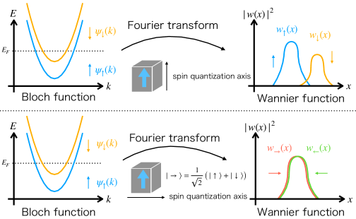
Figure 1: Schematic diagram of the process of constructing time-reversal symmetric Wannier functions. At the top, typical Wannier functions for up spin and down spin in a ferromagnetic material are depicted. In cases where the spin quantization axis for Wannierization aligns with the direction of magnetization, the spatial distributions of these Wannier functions do not match. At the bottom, time-reversal symmetric Wannier functions are shown. By orthogonalizing the spin quantization axis for Wannierization to the direction of magnetization, Wannier functions are obtained where the centers and spreads of the functions are paired, thereby matching.

2.3 Model Hamiltonian

The model Hamiltonian, dependent on the direction of magnetization, was derived following these steps: Initially, under the basis of TRS-WFs $\ket{j\mu\sigma}$, which are localized at position $j$ and specified by orbital $\mu$ and spin index $\sigma$, the matrix elements of the tight-binding Hamiltonian were decomposed into two terms: one symmetric and the other antisymmetric with respect to time reversal,

$$\matrixelement{j\mu\sigma}{H}{k\nu\sigma^{\prime}}=H_{j\mu\sigma;k\nu\sigma^{\prime}}=H_{j\mu\sigma;k\nu\sigma^{\prime}}^{s}+H_{j\mu\sigma;k\nu\sigma^{\prime}}^{a}.$$ (7)

Here, the time-reversal operator,

$$\Theta=-i\sigma^{y}K=\begin{pmatrix}0&-1\\ 1&0\end{pmatrix}K$$ (8)

is utilized, where $\sigma^{y}$ is the $y$ component of the Pauli matrices $\bm{\sigma}=(\sigma^{x},\sigma^{y},\sigma^{z})$ and the operator $K$ represents the complex conjugation.

Subsequently, the first term of Eq. (7) was further divided into two parts: one independent of spin, identified as the hopping integral $t$, and the other dependent on spin, recognized as the SOI represented by $\bm{\lambda}=(\lambda^{x},\lambda^{y},\lambda^{z})$ [39],

$$H_{j\mu\sigma;k\nu\sigma^{\prime}}^{s}=t_{j\mu;k\nu}\delta_{\sigma\sigma^{\prime}}+i(\bm{\lambda}_{j\mu;k\nu}\cdot\bm{\sigma})_{\sigma\sigma^{\prime}}.$$ (9)

It is easy to show that due to the properties of the time-reversal operator $\Theta$, all components of the hopping integral $t$ and the SOI $\bm{\lambda}$ are fundamentally real numbers. Similarly, the second term of Eq. (7) can be decomposed using Pauli matrices,

$$H_{j\mu\sigma;k\nu\sigma^{\prime}}^{a}=iM^{0}_{j\mu;k\nu}\delta_{\sigma\sigma^{\prime}}+(\bm{M}_{j\mu;k\nu}\cdot\bm{\sigma})_{\sigma\sigma^{\prime}}.$$ (10)

The components $M^{0}$ and $\bm{M}=(M^{x},M^{y},M^{z})$ of this term are also all real numbers.

In this study, we calculated the MCAE using three distinct methods. Method 1: The MCAE is calculated by rotating the magnetization in the tight-binding model defined in Eq. (10). In this approach, $H^{a}$ is approximated as the principal component of magnetization, $M^{z}_{i\mu;j\nu}$,

$$H_{j\mu\sigma;k\nu\sigma^{\prime}}^{a}\approx M^{z}_{i\mu;j\nu}(\sigma^{z})_{\sigma\sigma^{\prime}},$$ (11)

and rotated with the usual spinor rotation,

$$U_{\mathrm{s}}(\theta,\phi)=\begin{pmatrix}\cos\theta/2&e^{-i\phi}\sin\theta/2\\ -e^{i\phi}\sin\theta/2&\cos\theta/2\end{pmatrix}.$$ (12)

Indeed, when performing fully relativistic calculations, the assumption of collinear magnetization as the self-consistent spin density is justified up to the fourth-order perturbations of the SOI, according to the magnetic force theorem [40, 41]. We call this rotated tight-binding Hamiltonian as the tight-binding model with effective magnetization (TB-EM). The average value of the magnetization matrix elements discarded in the TB-EM method is defined as the computational error,

$$E_{\mathrm{err}}=\frac{1}{|H|}\sum_{jk}\sum_{\mu\nu}\sum_{\sigma\sigma^{\prime}}\{H_{j\mu\sigma;k\nu\sigma^{\prime}}^{a}-(M^{z}_{i\mu;j\nu}\sigma^{z})_{\sigma\sigma^{\prime}}\}$$ (13)

where $|H|$ represents the number of matrix elements in the Hamiltonian. This computational error, $E_{\mathrm{err}}$, corresponds to terms higher than the fourth-order perturbation of the SOI.

Method 2: Similar to Method 1, the MCAE is calculated by rotating the magnetization in the tight-binding model. However, this method retains all terms in Eq. (9) for the spinor rotation, and thus, we call this method as the tight-binding model with original magnetization (TB-OM) method.

Method 3: Here, the MCAE is calculated by rotating the magnetization in density functional theory (DFT) calculations. The tight-binding models are constructed for each of the DFT calculations and are utilized only for interpolating the energy of bands. We call this method as the DFT method. In the results section, we compare these three methods to discuss their validity and effectiveness.

2.4 Magnetocrystalline anisotropy energy

The MCAE, denoted as $\Delta E_{\mathrm{MCA}}$, is calculated based on the magnetic force theorem [40, 41], derived from the difference in band energies,

$$\Delta E_{\mathrm{MCA}}(\theta,\phi)=\frac{1}{N_{k}}\sum_{\bm{k}}\left(\sum_{n}f(\varepsilon_{n\bm{k}}^{(\theta,\phi)})\varepsilon_{n\bm{k}}^{(\theta,\phi)}-\sum_{m}f(\varepsilon_{m\bm{k}}^{(0,0)})\varepsilon_{m\bm{k}}^{(0,0)}\right).$$ (14)

Here, $n$ and $m$ are indices designating the bands, while $(\theta,\phi)$ represent the angles specifying the direction of magnetization. The number of $k$ points within the BZ is denoted by $N_{k}$. The terms $\varepsilon_{n\bm{k}}$ and $f(\varepsilon_{n\bm{k}})$ represent the energy at band $n$ and wave vector $\bm{k}$, and the Fermi distribution function respectively, where $f(\varepsilon)=\frac{1}{e^{\beta(\varepsilon-\mu)}+1}$.

The Fermi energy $\mu^{(\theta,\phi)}$, which depends on the direction of magnetization, is determined so as to satisfy the condition that the number of valence electrons per unit cell, $N_{\mathrm{elec}}$, remains constant at the temperature $T=0$,

$$N_{\mathrm{elec}}=\frac{1}{N_{k}}\sum_{\bm{k}}\sum_{n}f(\varepsilon_{n\bm{k}}^{(\theta,\phi)}).$$ (15)

2.5 Calculation details

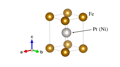
Figure 2: $\mathrm{L1_{0}}$ type crystal structure, where orange and grey spheres represent $\ce{Fe}$ and $\ce{Pt}$ ($\ce{Ni}$) atoms, respectively.

First-principles calculations program Quantum ESPRESSO [42, 43] based on plane-wave basis and pseudopotential methods were employed to obtain the Bloch states. Subsequently, a tight-binding model was created using Wannier90 program [4] in combination with SymWannier program [7], which takes into account the magnetic space group of the crystal. For the $\mathrm{L1_{0}}$ type crystal structure (Fig. 2), lattice constants were set as $a=2.728143~{}[$\mathrm{\SIUnitSymbolAngstrom}$]$, $c=3.778984~{}[$\mathrm{\SIUnitSymbolAngstrom}$]$ for $\ce{FePt}$, $a=2.506611~{}[$\mathrm{\SIUnitSymbolAngstrom}$]$, $c=3.581316~{}[$\mathrm{\SIUnitSymbolAngstrom}$]$ for $\ce{FeNi}$. The cutoff for the plane wave basis was set as $64.0~{}[\mathrm{Ry}]$, and for the electron density as $782.0~{}[\mathrm{Ry}]$. The exchange-correlation functional employed was the Perdew-Burke-Ernzerhof (PBE) formulation [44] of the generalized gradient approximation (GGA). Ultrasoft pseudopotentials from the PSLibrary [45] were utilized, with version 0.2.1 for $\ce{Fe}$ and version 0.1 for $\ce{Pt}$ and $\ce{Ni}$. According to the magnetic force theorem, SOI was incorporated during the non self-consistent field (NSCF) calculations.

Wannierization was carried out in a one-shot process, where the projection onto localized $s,p,d$ orbitals at the atomic center positions for each atom yielded 36 spinor Wannier Functions (WFs). For the $k$-mesh during Wannierization, a grid of $9\times 9\times 6$ was chosen for $\ce{FePt}$ and $9\times 9\times 7$ for $\ce{FeNi}$. From these, only $60$ inequivalent $k$ points under symmetry operations were utilized in the actual calculations for both cases. The inner energy window for disentanglement was carefully set to include the all $3d$ states of the magnetic element $\ce{Fe}$. For $\ce{FePt}$, a range of $[-1000,E_{F}+4]~{}[$\mathrm{e}\mathrm{V}$]$ was used, and for $\ce{FeNi}$, the range of $[-1000,E_{F}+5]~{}[$\mathrm{e}\mathrm{V}$]$ was used. The comparison between DFT and Wannier interpolated band structure is explained in A. Importantly, during Wannierization, the spin quantization axis (the $a$ axis) was set orthogonal to the direction of magnetization (the $c$ axis) in the first-principles calculations. This ensured that for both up and down spinors of the WFs, the differences in the centers of the WFs were less than $10^{-6}~{}[$\mathrm{\SIUnitSymbolAngstrom}$]$, and the differences in the spreads of the WFs were less than $10^{-8}~{}[$\mathrm{\SIUnitSymbolAngstrom}$^{2}]$ for all pairs.

3 Result

We first utilize the TB-EM method to increase the number of $k$-points in the BZ, to ensure the convergence of the MCAE. Following this, the dependence of MCAE on the chemical potential and SOI is examined. This involves comparing the three methods described in section 2.3, with a particular focus on assessing the validity of the TB-EM approach. Lastly, we compute the dependence of the MCAE on the angle of magnetization to derive the magnetic anisotropy constants.

3.1 $k$-mesh dependence

We initially employ $k$ interpolation with the TB-EM method to investigate the degree of convergence of the MCAE between the hard axis $[100]$ and the easy axis $[001]$, represented as $E_{[100]}-E_{[001]}$. The results are presented in Fig. 3. It is observed that for both $\ce{FePt}$ and $\ce{FeNi}$, increasing the number of $k$-points to $N_{k}=100^{3}$ ensures sufficient convergence of the MCAE within the range of computational error $E_{\mathrm{err}}$. In all subsequent calculations presented in this paper, we used a uniform $k$-point grid of $N_{k}=100^{3}$ points to determine the other dependence.

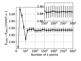
(a)

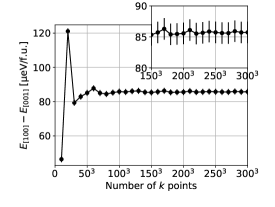
(b)

Figure 3: MCAE for (a) $\ce{FePt}$ and (b) $\ce{FeNi}$ with respect to the number of $k$-points. The error bars indicate the respective computational errors for each calculation. The MCAE converges to $2.885\pm 0.012~{}[\mathrm{meV}/f.u.]=17.21\pm 0.07~{}[\mathrm{MJ/m^{3}}]$ for FePt and $85.63\pm 2.71~{}[\mathrm{\mu eV}/f.u.]=0.610\pm 0.019~{}[\mathrm{MJ/m^{3}}]$ for FeNi, respectively.

3.2 Chemical potential dependence

We next focus on the difference between the TB-EM method (Method 1) and TB-OM method (Method 2), by calculating the chemical potential dependence of the MCAE and using the DFT method (Method 3) as a reference. The results, presented in Fig. 4, show that for $\ce{FePt}$, the TB-EM method closely matches the DFT result within the range of valence electron numbers from 16 to 20, when compared to the TB-OM method. The average difference between the TB-EM and DFT results is in the order of $10~{}[\mathrm{\mu eV}/f.u.]$. In contrast, for FeNi, both the TB-EM and TB-OM method reproduce a general trend of the DFT result, and the average differences with respect to the DFT results are in the order of $10~{}[\mathrm{\mu eV}/f.u.]$. This indicates that the limit of accuracy for MCAE calculations using the TB-EM method is in the order of $10~{}[\mathrm{\mu eV}/f.u.]$.

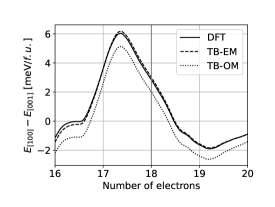
(a)

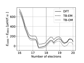
(b)

Figure 4: Chemical potential dependence of the MCAE for (a) $\ce{FePt}$ and (b) $\ce{FeNi}$ calculated using the three different methods. The horizontal axis represents the number of valence electrons, with the number 18 corresponding to the Fermi level. The DFT results (solid) are derived from Wannier $k$ interpolation oriented in two different directions. In all cases, the results with $100^{3}$ $k$-points are shown.

3.3 SOI dependence

Next, to conduct a more detailed comparison between the TB-EM and the TB-OM methods, we modify the magnitude of SOI in the second term of the model Hamiltonian in Eq. (9). This is done by uniformly scaling all elements of the SOI term with a real parameter $\lambda$. The results are illustrated in Fig. 5. In both $\ce{FePt}$ and $\ce{FeNi}$ cases, the MCAE obtained by the TB-EM method remains positive across all values of $\lambda$ in the range $0<\lambda<1.5$. In contrast, for the TB-OM method, there are regions where the MCAE becomes negative. Furthermore, in the TB-EM method, the MCAE exhibits a parabolic behavior in regions of smaller $\lambda$, aligning with the results of the second-order perturbation theory by Bruno [13] and van der Laan [14]. Additionally, the presence of a $\lambda^{4}$ term in regions of larger $\lambda$ suggests that the TB-EM method captures higher-order perturbation effects of SOI.

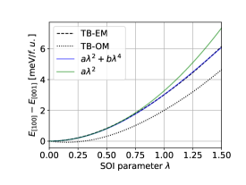
(a)

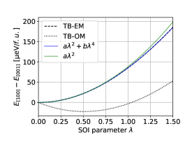
(b)

Figure 5: Dependence of the MCAE on the magnitude of SOI, denoted as $\lambda$, for (a) $\ce{FePt}$ and for (b) $\ce{FeNi}$. Here, $\lambda=0$ corresponds to the non-relativistic limit, while $\lambda=1$ represents the value in actual materials. The blue lines indicate the results of fitting with a fourth-order polynomial, and the green plots correspond to the situation when $b=0$. The fitting parameters of the fourth-order polynomial are $a=3.264\pm 0.012~{}[\mathrm{meV}/f.u.]$, $b=-0.249\pm 0.007~{}[\mathrm{meV}/f.u.]$ for $\ce{FePt}$ and $a=88.73\pm 0.11~{}[\mathrm{\mu eV}/f.u.]$, $b=-2.83\pm 0.07~{}[\mathrm{\mu eV}/f.u.]$ for $\ce{FeNi}$, respectively. In all cases, the results with $100^{3}$ $k$-points are shown.

3.4 Magnetization angle dependence

Finally, we calculate the detailed dependence of the MCAE on the magnetization direction $(\theta,\phi)$ using the TB-EM method. The angle dependence of MCAE for $\ce{FePt}$ and $\ce{FeNi}$ is depicted in Figs. 6 and 7, respectively. Furthermore, we employ a phenomenological formula for the angular dependence of MCAE,

$$\Delta E_{\mathrm{MCA}}(\theta,\phi)=K_{1}\sin^{2}\theta+K_{2}\sin^{4}\theta+K_{3}\sin^{4}\theta\cos 4\phi$$ (16)

to fit these data, from which the magnetic anisotropy constants $K_{i}$ are calculated. The results obtained are compiled in Tabs. 1 and 2, alongside values from prior theoretical and experimental studies.

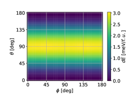
(a)

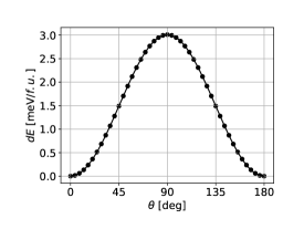
(b)

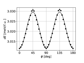
(c)

Figure 6: Dependence of the MCAE for $\ce{FePt}$ on the angular direction of magnetization $(\phi,\theta)$ measured from the $c$ axis. (a) For the full range of angles. (b) Along the line where the angle $(\phi,\theta)=(0,\theta)$. (c) Along the line where the angle $(\phi,\theta)=(\phi,\pi/2)$. In each of these cases, solid lines represent the fitting based on the phenomenological formula in Eq. (16). The results depicted in (a) were obtained using $60^{3}$ $k$-points, while those in (b) and (c) were derived using $100^{3}$ $k$-points. The fittings are conducted separately for (b) and (c).

According to Fig. 6, it can be seen that for $\ce{FePt}$, the angular dependence of the MCAE aligns well with Eq. (16). The result of fitting in Fig. 6(b) yields the magnetic anisotropy constants of $K_{1}=2.959~{}[\mathrm{meV}/f.u.]$ and $K_{2}=0.062~{}[\mathrm{meV}/f.u.]$, while that in Fig. 6(c) yields $K_{3}=-0.009~{}[\mathrm{meV}/f.u.]$. These results, when converted into standard units $[\mathrm{MJ/m^{3}}]$, are compared with previous studies in Tab. 1. Notably, there are no prior studies that have investigated the $\phi$ direction dependence given by $K_{3}$, while the values and ratios of $K_{1}$ and $K_{2}$ show good agreement with the theoretical results of Khan [25].

Table 1: Magnetic anisotropy constants of $\ce{FePt}$ are presented in units of $[\mathrm{MJ/m^{3}}]$. The upper section shows theoretical values, while the lower section shows experimental results.

Reference	$T$ [K]	$K_{2}/K_{1}$ [%]	$K_{U}$	$K_{1}$	$K_{2}$	$K_{3}$
this study	0	2.1	17.964	17.648	0.370	-0.054
Daalderop $et~{}al.$ (1991) [15]	0		20.4
Sakuma (1994) [16]	0		16.3
Solovyev $et~{}al.$ (1995) [17]	0		19.6
Oppeneer (1998) [18]	0		15.9
Galanakis $et~{}al.$ (2000) [19]	0		22.1
Ravindran $et~{}al.$ (2001) [20]	0		15.52
Staunton $et~{}al.$ (2004) [21]	0		9.523
Burkert $et~{}al.$ (2005) [22]	0		16.12
Lu $et~{}al.$ (2010) [23]	0		16.62
Kosugi $et~{}al.$ (2014) [24]	0		18.25
Khan $et~{}al.$ (2016) [25]	0		16.59 (Wien2k)
Khan $et~{}al.$ (2016) [25]	0	3.1	18.17 (SPR-KKR)	17.51	0.54
Ke (2019) [26]	0		14.51
Alsaad $et~{}al.$ (2020) [27]	0		7.6
Okamoto $et~{}al.$ (2002) [33]	Room T.	31.5		2.13	0.67
Inoue $et~{}al.$ (2006) [34]	5	1.8	6.9	7.4	0.13
Richter $et~{}al.$ (2011) [35]	850	9		2.93
Goll $et~{}al.$ (2013) [46]	Room T.		6
Ikeda $et~{}al.$ (2017) [47]	Room T.		4.6
Ono $et~{}al.$ (2018) [36]	Room T.	44	3.4	0.9	0.4
Saito $et~{}al.$ (2021) [48]	Room T.		$1.8\sim 2.3$

In contrast to the case of $\ce{FePt}$, the angular dependence of the MCAE for $\ce{FeNi}$, especially in the $\phi$ direction on the order of $0.1~{}[\mathrm{\mu eV}/f.u.]$, is obscure by computational error as shown in Fig. 7. While the positions of the peaks are accurately captured, the curve does not replicate the expected cosine curve. The magnetic anisotropy constants fitted using Eq. (16) as shown in Figs. 7(b) and (c) are found to be $K_{1}=86.681~{}[\mathrm{\mu eV}/f.u.]$, $K_{2}=-0.772~{}[\mathrm{\mu eV}/f.u.]$, and $K_{3}=-0.082~{}[\mathrm{\mu eV}/f.u.]$. As shown in Tab. 2, the previous study of Woodgate [31] concluded that $K_{3}$ is positive. This suggests that the easy axis direction in the $a$-$b$ plane for $\ce{FeNi}$ is along $[110]$ rather than $[100]$. However, our calculations indicate that, similar to $\ce{FePt}$, the easy axis in the $a$-$b$ plane for $\ce{FeNi}$ is also in the $[100]$ (or $[010]$) direction.

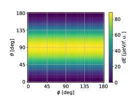
(a)

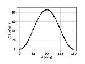
(b)

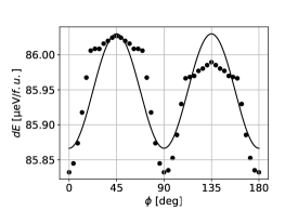
(c)

Figure 7: Dependence of the MCAE for $\ce{FeNi}$ on the angular direction of magnetization $(\phi,\theta)$ measured from the $c$ axis. (a) For the full range of angles. (b) Along the line where the angle $(\phi,\theta)=(0,\theta)$. (c) Along the line where the angle $(\phi,\theta)=(\phi,\pi/2)$. In each of these cases, solid lines represent the fitting based on the phenomenological formula, as expressed in Eq. (16). The results depicted in (a) were obtained using $60^{3}$ $k$-points, while those in (b) and (c) were derived using $100^{3}$ $k$-points. The fittings are conducted separately for (b) and (c).

Table 2: Magnetic anisotropy constants of $\ce{FeNi}$ are presented in units of $[\mathrm{MJ/m^{3}}]$. The upper section shows theoretical values, while the lower section shows experimental results. The table includes an excerpt from the sources [30, 31].

Reference	$T$ [K]	$K_{U}$	$K_{1}$	$K_{2}$	$K_{3}$
this study	0	0.61	0.6172	-0.0055	-0.0006
Ravindran $et~{}al.$ (2001) [20]	0	0.54
Miura $et~{}al.$ (2013) [28]	0	0.56
Edström $et~{}al.$ (2014) [29]	0	0.48 (Wien2k)
Edström $et~{}al.$ (2014) [29]	0	0.77 (SPR-KKR)
Qiao $et~{}al.$ (2019) [30]	0	$0.52\pm 0.05$
Ke (2019) [26]	0	0.47
Woodgate $et~{}al.$ (2023) [31]	0	0.96	0.9582	-0.0008	0.0001
Néel $et~{}al.$ (1964) [37]	293	0.55	0.32	0.23
Paulevé $et~{}al.$ (1968) [38]	Room T.	0.55	0.3	0.17	0.08
Shima $et~{}al.$ (2007) [49]	Room T.	0.63
Mizuguchi $et~{}al.$ (2011) [50]	Room T.	0.58
Kojima $et~{}al.$ (2011) [51]	Room T.	$0.5\pm 0.1$
Frisk $et~{}al.$ (2017) [52]	300	$\sim 0.35$
Ito $et~{}al.$ (2023) [53]	Room T.	0.55
Nishio $et~{}al.$ (2023) [54]	300	0.63

4 Conclusion

In our research, we developed the TB-EM method, based on the SAWFs. By investigating the dependence of the MCAE on the number of $k$ points, chemical potential and SOI, we demonstrated that the TB-EM method provides a valid effective Hamiltonian with an accuracy of the order of approximately $10~{}[\mathrm{\mu eV}/f.u.]$. Furthermore, using the TB-EM method, we determined the magnetic anisotropy constants for $\ce{FePt}$ and $\ce{FeNi}$. This methodology holds the potential for low-cost computation of various physical quantities dependent on the direction of magnetization.

5 Acknowledgement

This work was supported by JSPS KAKENHI Grant No. 21H01003, 21H04437, 22K03447, and 23H04869, JST-Mirai Program (JPMJMI20A1), Center for Science and Innovation in Spintronics (CSIS), Tohoku University and GP-Spin at Tohoku University.

Appendix A Band structure and density of states

Figures 8 and 9 display the band structures and density of states for $\ce{FePt}$ and $\ce{FeNi}$, respectively. As mentioned in section 2.5, the inner windows for Wannierization were $[-1000,E_{F}+4]~{}[$\mathrm{e}\mathrm{V}$]$ and $[-1000,E_{F}+5]~{}[$\mathrm{e}\mathrm{V}$]$ for each case. These ranges effectively encompass the states of the $\ce{Fe}$ $3d$ for both up and down spin.

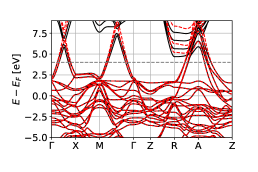
(a)

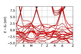
(b)

Figure 8: Comparison between DFT band structure (black) and Wannier interpolated band structure (red) for (a) $\ce{FePt}$ and (b) (a) $\ce{FeNi}$. In both cases, dashed lines represent the maximum values of the inner window.

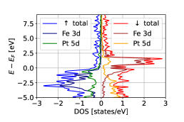
(a)

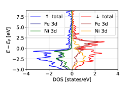
(b)

Figure 9: Density of states for (a) $\ce{FePt}$ and (b) $\ce{FeNi}$.

References

- [1] N. Marzari, D. Vanderbilt, Maximally localized generalized wannier functions for composite energy bands, Phys. Rev. B 56 (1997) 12847.
- [2] I. Souza, N. Marzari, D. Vanderbilt, Maximally localized wannier functions for entangled energy bands, Phys. Rev. B 65 (2001) 035109.
- [3] N. Marzari, A. A. Mostofi, J. R. Yates, I. Souza, D. Vanderbilt, Maximally localized wannier functions: Theory and applications, Rev. Mod. Phys. 84 (2012) 1419.
- [4] G. Pizzi, V. Vitale, R. Arita, S. Blügel, F. Freimuth, G. Géranton, M. Gibertini, D. Gresch, C. Johnson, T. Koretsune, J. Ibañez-Azpiroz, H. Lee, J.-M. Lihm, D. Marchand, A. Marrazzo, Y. Mokrousov, J. I. Mustafa, Y. Nohara, Y. Nomura, L. Paulatto, S. Poncé, T. Ponweiser, J. Qiao, F. Thöle, S. S. Tsirkin, M. Wierzbowska, N. Marzari, D. Vanderbilt, I. Souza, A. A. Mostofi, J. R. Yates, Wannier90 as a community code: new features and applications, J. Phys. Condens. Matter 32 (2020) 165902.
- [5] J. R. Yates, X. Wang, D. Vanderbilt, I. Souza, Spectral and fermi surface properties from wannier interpolation, Phys. Rev. B 75 (2007) 195121.
- [6] R. Sakuma, Symmetry-adapted wannier functions in the maximal localization procedure, Phys. Rev. B 87 (2013) 235109.
- [7] T. Koretsune, Construction of maximally-localized wannier functions using crystal symmetry, Comput. Phys. Commun. 285 (2023) 108645.
- [8] Y. Miura, J. Okabayashi, Understanding magnetocrystalline anisotropy based on orbital and quadrupole moments, J. Phys. Condens. Matter 34 (2022) 473001.
- [9] S. Bhatti, R. Sbiaa, A. Hirohata, H. Ohno, S. Fukami, S. N. Piramanayagam, Spintronics based random access memory: a review, Mater. Today 20 (2017) 530.
- [10] A. Hashimoto, S. Saito, M. Takahashi, A soft magnetic underlayer with negative uniaxial magnetocrystalline anisotropy for suppression of spike noise and wide adjacent track erasure in perpendicular recording media, J. Appl. Phys. 99 (2006) 08Q907.
- [11] K. Yoshida, M. Yokoe, Y. Ishikawa, Y. Kanai, Spin torque oscillator with negative magnetic anisotropy materials for MAMR, IEEE Trans. Magn. 46 (2010) 2466.
- [12] M. Igarashi, Y. Suzuki, Y. Sato, Oscillation feature of planar Spin-Torque oscillator for Microwave-Assisted magnetic recording, IEEE Trans. Magn. 46 (2010) 3738.
- [13] P. Bruno, Tight-binding approach to the orbital magnetic moment and magnetocrystalline anisotropy of transition-metal monolayers, Phys. Rev. B 39 (1989) 865.
- [14] G. van der Laan, Microscopic origin of magnetocrystalline anisotropy in transition metal thin films, J. Phys. Condens. Matter 10 (1998) 3239.
- [15] G. H. Daalderop, P. J. Kelly, M. F. Schuurmans, Magnetocrystalline anisotropy and orbital moments in transition-metal compounds, Phys. Rev. B 44 (1991) 12054.
- [16] A. Sakuma, First principle calculation of the magnetocrystalline anisotropy energy of FePt and CoPt ordered alloys, J. Phys. Soc. Jpn. 63 (1994) 1422.
- [17] I. V. Solovyev, IV, P. H. Dederichs, I. Mertig, I, Origin of orbital magnetization and magnetocrystalline anisotropy in TX ordered alloys (where T=Fe,Co and X=Pd,Pt), Phys. Rev. B 52 (1995) 13419.
- [18] P. M. Oppeneer, Magneto-optical spectroscopy in the valence-band energy regime: relationship to the magnetocrystalline anisotropy, J. Magn. Magn. Mater. 188 (1998) 275.
- [19] I. Galanakis, M. Alouani, H. Dreyssé, Perpendicular magnetic anisotropy of binary alloys: A total-energy calculation, Phys. Rev. B 62 (2000) 6475.
- [20] P. Ravindran, A. Kjekshus, H. Fjellvåg, P. James, L. Nordström, B. Johansson, O. Eriksson, Large magnetocrystalline anisotropy in bilayer transition metal phases from first-principles full-potential calculations, Phys. Rev. B 63 (2001) 144409.
- [21] J. B. Staunton, S. Ostanin, S. S. A. Razee, B. L. Gyorffy, L. Szunyogh, B. Ginatempo, E. Bruno, Temperature dependent magnetic anisotropy in metallic magnets from an ab initio electronic structure theory: L10-ordered FePt, Phys. Rev. Lett. 93 (2004) 257204.
- [22] T. Burkert, O. Eriksson, S. I. Simak, A. V. Ruban, B. Sanyal, L. Nordström, J. M. Wills, Magnetic anisotropy of 10 FePt and Fe-xMnxPt, Phys. Rev. B 71 (2005) 134411.
- [23] Z. Lu, R. V. Chepulskii, W. H. Butler, First-principles study of magnetic properties of l10-ordered MnPt and FePt alloys, Phys. Rev. B 81 (2010) 094437.
- [24] T. Kosugi, T. Miyake, S. Ishibashi, Second-Order perturbation formula for magnetocrystalline anisotropy using orbital angular momentum matrix, J. Phys. Soc. Jpn. 83 (2014) 044707.
- [25] S. Ayaz Khan, P. Blaha, H. Ebert, J. Minár, O. Šipr, Magnetocrystalline anisotropy of FePt: A detailed view, Phys. Rev. B 94 (2016) 144436.
- [26] L. Ke, Intersublattice magnetocrystalline anisotropy using a realistic tight-binding method based on maximally localized wannier functions, Phys. Rev. B 99 (2019) 054418.
- [27] A. Alsaad, A. A. Ahmad, T. S. Obeidat, Structural, electronic and magnetic properties of the ordered binary FePt, MnPt, and CrPt3 alloys, Heliyon 6 (2020) e03545.
- [28] Y. Miura, S. Ozaki, Y. Kuwahara, M. Tsujikawa, K. Abe, M. Shirai, The origin of perpendicular magneto-crystalline anisotropy in L10-FeNi under tetragonal distortion, J. Phys. Condens. Matter 25 (2013) 106005.
- [29] A. Edström, J. Chico, A. Jakobsson, A. Bergman, J. Rusz, Electronic structure and magnetic properties of l10 binary alloys, Phys. Rev. B 90 (2014) 014402.
- [30] J. Qiao, W. Zhao, Efficient technique for ab-initio calculation of magnetocrystalline anisotropy energy, Comput. Phys. Commun. 238 (2019) 203.
- [31] C. D. Woodgate, C. E. Patrick, L. H. Lewis, J. B. Staunton, Revisiting Néel 60 years on: The magnetic anisotropy of L10 FeNi (tetrataenite), J. Appl. Phys. 134 (2023) 163905.
- [32] S. Yamashita, A. Sakuma, First-Principles study for finite temperature magnetrocrystaline anisotropy of L10-Type ordered alloys, J. Phys. Soc. Jpn. 91 (2022) 093703.
- [33] S. Okamoto, N. Kikuchi, O. Kitakami, T. Miyazaki, Y. Shimada, K. Fukamichi, Chemical-order-dependent magnetic anisotropy and exchange stiffness constant of FePt (001) epitaxial films, Phys. Rev. B 66 (2002) 024413.
- [34] K. Inoue, H. Shima, A. Fujita, K. Ishida, K. Oikawa, K. Fukamichi, Temperature dependence of magnetocrystalline anisotropy constants in the single variant state of l10-type FePt bulk single crystal, Appl. Phys. Lett. 88 (2006) 102503.
- [35] H. J. Richter, O. Hellwig, S. Florez, C. Brombacher, M. Albrecht, Anisotropy measurements of FePt thin films, J. Appl. Phys. 109 (2011) 07B713.
- [36] T. Ono, N. Kikuchi, S. Okamoto, O. Kitakami, T. Shimatsu, Novel torque magnetometry for uniaxial anisotropy constants of thin films and its application to FePt granular thin films, Appl. Phys. Express 11 (2018) 033002.
- [37] L. Néel, J. Pauleve, R. Pauthenet, J. Laugier, others, Magnetic properties of an iron—nickel single crystal ordered by neutron bombardment, J. Appl. Phys. 35 (1964) 873.
- [38] J. Paulevé, A. Chamberod, K. Krebs, others, Magnetization curves of Fe–Ni (50–50) single crystals ordered by neutron irradiation with an applied magnetic field, J. Appl. Phys. 39 (1968) 989.
- [39] K. Kurita, T. Koretsune, Systematic first-principles study of the on-site spin-orbit coupling in crystals, Phys. Rev. B 102 (2020) 045109.
- [40] M. Weinert, R. E. Watson, J. W. Davenport, Total-energy differences and eigenvalue sums, Phys. Rev. B 32 (1985) 2115.
- [41] X. Wang, D.-S. Wang, R. Wu, A. J. Freeman, Validity of the force theorem for magnetocrystalline anisotropy, J. Magn. Magn. Mater. 159 (1996) 337.
- [42] P. Giannozzi, S. Baroni, N. Bonini, M. Calandra, R. Car, C. Cavazzoni, D. Ceresoli, G. L. Chiarotti, M. Cococcioni, I. Dabo, A. D. Corso, S. de Gironcoli, S. Fabris, G. Fratesi, R. Gebauer, U. Gerstmann, C. Gougoussis, A. Kokalj, M. Lazzeri, L. Martin-Samos, N. Marzari, F. Mauri, R. Mazzarello, S. Paolini, A. Pasquarello, L. Paulatto, C. Sbraccia, S. Scandolo, G. Sclauzero, A. P. Seitsonen, A. Smogunov, P. Umari, R. M. Wentzcovitch, QUANTUM ESPRESSO: a modular and open-source software project for quantum simulations of materials, J. Phys. Condens. Matter 21 (2009) 395502.
- [43] P. Giannozzi, O. Andreussi, T. Brumme, O. Bunau, M. Buongiorno Nardelli, M. Calandra, R. Car, C. Cavazzoni, D. Ceresoli, M. Cococcioni, N. Colonna, I. Carnimeo, A. Dal Corso, S. de Gironcoli, P. Delugas, R. A. DiStasio, Jr, A. Ferretti, A. Floris, G. Fratesi, G. Fugallo, R. Gebauer, U. Gerstmann, F. Giustino, T. Gorni, J. Jia, M. Kawamura, H.-Y. Ko, A. Kokalj, E. Küçükbenli, M. Lazzeri, M. Marsili, N. Marzari, F. Mauri, N. L. Nguyen, H.-V. Nguyen, A. Otero-de-la Roza, L. Paulatto, S. Poncé, D. Rocca, R. Sabatini, B. Santra, M. Schlipf, A. P. Seitsonen, A. Smogunov, I. Timrov, T. Thonhauser, P. Umari, N. Vast, X. Wu, S. Baroni, Advanced capabilities for materials modelling with quantum ESPRESSO, J. Phys. Condens. Matter 29 (2017) 465901.
- [44] J. P. Perdew, K. Burke, M. Ernzerhof, Generalized gradient approximation made simple, Phys. Rev. Lett. 77 (1996) 3865.
- [45] A. Dal Corso, Pseudopotentials periodic table: From H to pu, Comput. Mater. Sci. 95 (2014) 337.
- [46] D. Goll, T. Bublat, Large-area hard magnetic L10 -FePt and composite L10 -FePt based nanopatterns, Phys. Status Solidi 210 (2013) 1261.
- [47] K. Ikeda, T. Seki, G. Shibata, T. Kadono, K. Ishigami, Y. Takahashi, M. Horio, S. Sakamoto, Y. Nonaka, M. Sakamaki, K. Amemiya, N. Kawamura, M. Suzuki, K. Takanashi, A. Fujimori, Magnetic anisotropy of l10-ordered FePt thin films studied by fe and pt l2,3-edges x-ray magnetic circular dichroism (2017).
- [48] T. Saito, K. K. Tham, R. Kushibiki, T. Ogawa, S. Saito, Separate quantitative evaluation of degree of order and perpendicular magnetic anisotropy for disorder and order portion in FePt granular films, AIP Adv. 11 (2021) 015310.
- [49] T. Shima, M. Okamura, S. Mitani, K. Takanashi, Structure and magnetic properties for l10-ordered FeNi films prepared by alternate monatomic layer deposition, J. Magn. Magn. Mater. 310 (2007) 2213.
- [50] M. Mizuguchi, T. Kojima, M. Kotsugi, others, Artificial fabrication and order parameter estimation of l10-ordered FeNi thin film grown on a AuNi buffer layer, J. Magn. Soc. Jpn 35 (2011) 370–373.
- [51] T. Kojima, M. Mizuguchi, K. Takanashi, L10-ordered FeNi film grown on Cu-Ni binary buffer layer, J. Phys. Conf. Ser. 266 (2011) 012119.
- [52] A. Frisk, T. P. A. Hase, P. Svedlindh, E. Johansson, G. Andersson, Strain engineering for controlled growth of thin-film FeNi l10, J. Phys. D Appl. Phys. 50 (2017) 085009.
- [53] K. Ito, T. Ichimura, M. Hayashida, T. Nishio, S. Goto, H. Kura, R. Sasaki, M. Tsujikawa, M. Shirai, T. Koganezawa, M. Mizuguchi, Y. Shimada, T. J. Konno, H. Yanagihara, K. Takanashi, Fabrication of l10-ordered FeNi films by denitriding FeNiN(001) and FeNiN(110) films, J. Alloys Compd. 946 (2023) 169450.
- [54] T. Nishio, K. Ito, H. Kura, K. Takanashi, H. Yanagihara, Uniaxial magnetic anisotropy of L10-FeNi films with island structures on LaAlO3(110) substrates by nitrogen insertion and topotactic extraction, J. Alloys Compd. 976 (2024) 172992.