Analyzing Downlink Coverage in Clustered Low Earth Orbit Satellite Constellations: A Stochastic Geometry Approach
Abstract
Satellite networks are emerging as vital solutions for global connectivity beyond 5G. As companies such as SpaceX, OneWeb, and Amazon are poised to launch a large number of satellites in low Earth orbit, the heightened inter-satellite interference caused by mega-constellations has become a significant concern. To address this challenge, recent works have introduced the concept of satellite cluster networks where multiple satellites in a cluster collaborate to enhance the network performance. In order to investigate the performance of these networks, we propose mathematical analyses by modeling the locations of satellites and users using Poisson point processes, building on the success of stochastic geometry-based analyses for satellite networks. In particular, we suggest the lower and upper bounds of the coverage probability as functions of the system parameters, including satellite density, satellite altitude, satellite cluster area, path loss exponent, and Nakagami parameter . We validate the analytical expressions by comparing them with simulation results. Our analyses can be used to design reliable satellite cluster networks by effectively estimating the impact of system parameters on the coverage performance.
Index Terms:
Satellite communications, mega-constellations, satellite cluster, stochastic geometry, coverage probability.I Introduction
Satellite communications have garnered interest as a promising solution to achieve ubiquitous connectivity. According to the International Telecommunication Union report [1], nearly half of the global population remains unconnected. Satellites are expected to address this connectivity gap, offering a viable solution that alleviates the cost burden faced by telecom operators when deploying terrestrial base stations [2]. Traditionally, geostationary orbit (GEO) satellites were the primary choice for satellite networks due to the extensive coverage facilitated by their high altitudes. However, the extremely high altitudes of GEO satellites present challenges such as high latency and low area spectral efficiency, making them less suitable for 5G applications. The industry has shifted towards adopting low Earth orbit (LEO) satellites to reduce latency, increase service density, and facilitate cost-effective launches [3, 4, 5]. Companies like SpaceX, OneWeb, and Amazon are planning to deploy large constellations in LEOs, often referred to as mega-constellations [6]. However, in mega-constellations, launching additional satellites does not necessarily increase throughput and could even lead to performance degradation due to severe inter-satellite interference. To tackle this challenge, satellite cooperation concepts such as LEO remote sensing [7] and satellite clusters [8],[9] have been introduced to manage satellite networks effectively and mitigate inter-satellite interference.
As mega-constellations complicate simulation-based network performance analyses, the need for new tools arises for effective assessment. Stochastic geometry is introduced to mathematically analyze performance, modeling the random behavior of nodes in wireless networks, including base stations and users, through point processes such as binomial point processes (BPPs) or Poisson point processes (PPPs) [10]. Previous studies [11, 12, 13, 14, 15, 16] have conducted stochastic geometry-based analyses for wireless networks using various performance metrics for terrestrial networks. A framework for modeling wireless networks was proposed in [11], addressing the outage probability, network throughput, and capacity. In [12], the distribution of base stations modeled by a PPP was compared to the actual distribution in cellular networks, and the coverage probability and average rate were evaluated. The authors in [13] modeled downlink heterogeneous cellular networks with the PPP and analyzed the coverage probability and average rate. In [14], the coverage probability for uplink cellular networks modeled by the PPP was studied. The authors in [15] derived the downlink coverage probability considering base station cooperation within the PPP framework. A BPP model for a cache-enabled networks was used to characterize the downlink coverage probability and network spectral efficiency in [16].
Building on stochastic geometry-based analyses in terrestrial networks, recent works have extended its application to satellite networks. Given the envisaged prevalence of large-scale satellite constellations, it is crucial to analyze the network performance in scenarios where multiple satellites serve a user, moving beyond a single-satellite setup. In this work, we focus on satellite cluster networks, a pertinent solution in mega-constellations, and employ stochastic geometry to characterize the coverage probability, providing an effective means of estimating the impact of system parameters.
I-A Related Works
The recent works [17, 18, 19, 20, 21, 22, 23, 24, 25] have utilized the stochastic geometry to evaluate the system-level performance of satellite networks, focusing on scenarios where each user is served by a single satellite at a given time. Some of these works [17, 18, 19] modeled the distribution of satellite locations on the surface of a sphere using a BPP, i.e., the number of satellites distributed in a certain area follows the binomial distribution. In [17], the coverage probability and average achievable rate were evaluated, and guidelines for selecting the system parameters such as the altitudes and the number of frequency channels were proposed. The authors in [18] derived the outage probability considering satellite antenna patterns and practical channels modeled by the shadowed-Rician fading. In addition, the coverage performance was investigated in [19] for a scenario where satellite gateways that serve as relays between the users and the LEO satellites are deployed on the ground.
Other works [20, 21, 22, 23] modeled the distribution of satellite locations using a PPP, i.e., the number of nodes is randomly determined according to the Poisson distribution. While it is conventionally applied in an infinite two-dimensional area, the recent finding has demonstrated that PPPs can effectively characterize node distribution even in finite space. In particular, the authors in [20] showed that a PPP could effectively capture the actual Starlink constellation in terms of the number of visible satellites, and derived the coverage probability. In [21], the coverage probability was derived based on the contact distance distribution. The work [22] dealt the problem that determines the optimal satellite altitude to maximize the downlink coverage probability. In [23], a non-homogeneous PPP was used to model the varying satellite density according to latitudes, and the coverage probability and average achievable data rate were derived. Furthermore, the other works [24, 25] analyzed satellite networks considering orbit geometry. In [24], a PPP was employed to model the distribution of satellites in orbits. To capture the geometric characteristics of satellites with orbits that may vary in altitude, a framework using a Cox point process was suggested, and the outage probability was investigated in [25]. From these works, we conclude that point processes can successfully model actual satellite constellations, and analytical results based on stochastic geometry can effectively estimate the actual performance. However, these performance analyses have been conducted solely under the scenario where a single satellite serves a user.
The proliferation of satellites underscores the necessity for a theoretical understanding of system parameters to design networks effectively. In light of this, our stochastic geometry-based analyses shift the focus from scenarios where a single satellite serves to those involving multiple satellites, examining the impact of system parameters on network performance.
I-B Contributions
We focus on satellite networks where multiple satellites in a cluster area collaborate to serve a user, while satellites outside this area operate as interfering nodes. To assess the network performance, we employ stochastic geometry to model the locations of satellites and users. In particular, the satellite locations follow a homogeneous PPP on the surface of a sphere defined by the satellite orbit radius, and the user locations also follow a homogeneous PPP on the surface of a sphere defined by the Earth radius.
The main contributions are summarized as follows:
-
•
Due to joint transmissions via cooperative satellites to mitigate the inter-satellite interference, managing compound terms, i.e., the accumulated cluster power and interference power, is necessary for deriving the coverage probability. To handle these terms simultaneously, we leverage properties that the sum over Poisson processes on a finite sphere surface can be approximated as a single random variable: the Gamma random variable. This enables us to determine the shape and scale parameters of these approximated Gamma random variables.
-
•
Using stochastic geometry, we derive the lower and upper bounds of the coverage probability through a finite number of operations. For the specific case where the Nakagami parameter is configured to 1, i.e., Rayleigh fading, we deduce simplified closed-form expressions. Additionally, we introduce an equation that accommodates the influence of round-up and -down operations undertaken during the derivation of bounds by considering the relative distances. This heuristically derived equation closely aligns with actual results and provides a more direct explanation of the impact of system parameters on the coverage probability compared to the bounds.
-
•
Finally, we demonstrate that the derived lower and upper bounds of the coverage probability effectively encapsulate the simulations, and the heuristic approach also exhibits fair proximity. Moreover, we conduct analyses on the influence of the satellite cluster area on the coverage probability.
I-C Organizations
The remainder of the paper is organized as follows. We describe the system model in Section II. Baseline preliminaries for deriving the lower and upper bounds of the coverage probability are presented in Section III. In Section IV, we derive the lower and upper bounds of the coverage probability. In Section V, simulation results validate the analytical expressions and analyze the impact of satellite clustering on the coverage probability. Finally, conclusions follow in Section VI.
Notation
Sans-serif letters () denote random variables while serif letters () denote their realizations or scalar variables. Lower boldface symbols () denote column vectors. and denote the expectation and variance. denotes the Euclidean norm. and are used to denote the probability density function (PDF) and the cumulative density function (CDF). The Laplace transform of is defined as . denotes probability. is used to denote the Gamma distribution with the shape parameter and scale parameter . The Gamma function is defined as . Specifically, for positive integer , the Gamma function is defined as . is the Gauss’s hypergeometric function. and denote the round-up and -down operations.
II System Model
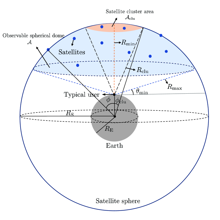
We consider a downlink satellite network depicted in Fig. 1. Satellites are located on a sphere with radius according to a homogeneous spherical Poisson point process (SPPP) where , , is the position of the satellite in a spherical coordinate system with elevation and azimuth angles spanning from to and to , respectively. The number of total satellites, , follows the Poisson distribution with density . Single-antenna users, positioned on the Earth’s surface with radius , are also distributed according to a homogeneous SPPP, denoted as , where is the number of total users on the Earth, which follows the Poisson distribution with density . According to the Slivnyak’s theorem [10], we focus on a typical user located at for our downlink performance analyses without loss of generality.
II-A Observable Spherical Dome and Cluster Area
Given that satellites below a specified elevation angle may be invisible to the typical user, we introduce the elevation angle to define the observable spherical dome . To take the visibility constraint into account, we define the maximum distance to the satellites in the observable spherical dome as , which is given by
| (1) |
using the law of cosines. Then we calculate the surface area of the observable spherical dome, , using the Archimedes’ Hat box theorem as [26]
| (2) |
To define the satellite cluster area where the satellites in the region cooperatively serve a user, we utilize the polar angle , which represents the maximum zenith angle of the multiple satellites in the cluster area as shown in Fig. 1. The maximum distance from the typical user to the cluster area, , and the surface area of the cluster are then respectively given by
| (3) |
| (4) |
Additionally, we define the minimum distance to the cluster area as .
II-B Channel Model
II-B1 Propagation Model
Our model encompasses large- and small-scale fading to characterize channel quality variation. Large-scale fading is captured using a path loss model, denoted as for , which depends on the distance and the path loss exponent [17], [20]. For small-scale fading, we model the line-of-sight (LOS) properties, which are attributed to the high altitude of satellites, with the Nakagami- distribution. This distribution captures the LOS effect by adjusting the parameter and provides analytical tractability. The PDF of the power of small-scale channel fading from the satellite to the typical user is expressed as
| (5) |
where and .
II-B2 Antenna Gain
We assume that the satellites’ beams have directional radiation patterns, while the antenna of the typical user employs an isotropic radiation pattern. Satellites maintain the boresight of their beams in the direction of the subsatellite point. With a sufficiently small cluster area, we assume the satellites in the cluster area can keep their mainlobes directed at the typical user. Conversely, satellites outside the cluster area have the typical user within the range of the sidelobe due to the narrow beamwidth for long-distance satellite communications [27]. This leads to higher antenna gain for satellites in the cluster area and a lower gain for satellites outside the cluster area. Based on the two-lobe approximation using Dolph-Chebyshev beamforming weights [28], the sectored antenna gain model for the satellite [20],[29],[30],[31] is defined as
| (6) |
where is the carrier frequency, and is the speed of light. The transmit antenna gain is determined by the satellite location, with for those in the cluster area and for those outside. The typical user’s receive antenna gain is denoted as .
III Mathematical Preliminaries
To derive the coverage probability, it is necessary to establish a basic performance metric and mathematical preliminaries. We assume an interference-limited network and employ the signal-to-interference ratio (SIR) as a performance metric. This choice encapsulates the scenario where interference becomes predominant with the increasing number of satellites, making noise negligible. We also approximate the accumulated received power from the satellites within and outside the cluster area as Gamma random variables, consolidating these compound terms into their respective single random variables.
III-A Performance Metric
We define the SIR under the condition that satellites in the cluster area transmit the signal using non-coherent joint transmission to serve the typical user [15]. The SIR at the typical user, located at , is expressed as
| (7) |
where denotes the outside of the cluster area, and represents the transmit power. In (7), the numerator and denominator indicate the accumulated power from the satellites within and outside the cluster area. For analytical simplicity, we normalize these two terms by the transmit power . The accumulated cluster power is then characterized as
| (8) |
while the accumulated interference power is given by
| (9) |
III-B Gamma Approximation
Before deriving the coverage probability, we first approximate the statistics of the sum of random variables on the state space of a Poisson process. Previous studies [32], [33] demonstrated the appropriateness of the Gamma random variable for closely modeling the statistics of the accumulated interference power in terrestrial networks. Building upon these findings, we approximate both the accumulated interference power and the accumulated cluster power in the context of satellite networks.
Proposition 1.
The accumulated interference power can be approximated as a Gamma random variable . The shape parameter and scale parameter of are obtained as
| (10) |
| (11) |
Proof.
See Appendix A. ∎
We also consider the accumulated cluster power as a Gamma random variable . The shape parameter and scale parameter are given by
| (12) |
| (13) |
These parameters are obtained through the same process as in the aforementioned proposition.
The coverage probability is derived using the statistical properties of or . When deriving the coverage probability based on , we can directly incorporate without employing Gamma approximation. On the contrary, when the coverage probability is based on , we can consider directly without its approximation. For the following section, we elaborate on the coverage probability using instead of .
IV Coverage Probability
In this section, we propose the coverage probability of the satellite cluster network, with a focus on downlink satellite cooperation in the cluster area. We utilize the SIR that incorporates joint transmissions in the cluster area, as defined in Section III-A, and apply the Gamma approximation outlined in Section III-B to derive the lower and upper bounds for the coverage probability. We assume the mutual independence of the processes governing the distribution of satellites within and outside the cluster area, given their distinct spatial regions.
The coverage probability in the interference-limited regime is the probability that the SIR at the typical user is greater than or equal to a threshold . This probability is derived as
| (14) | ||||
| (15) |
where is the SIR threshold. To derive the coverage probability based on (14), we use the parameters given in (10) and (11) to consider the CDF of the approximated Gamma random variable . Similarly, when obtaining the coverage probability based on (15), we utilize the parameters provided in (12) and (13) to incorporate the complementary CDF of the corresponding approximated Gamma random variable . For the remainder of this section, we opt for (14) to attain the coverage probability with the approximated Gamma random variable .
In order to obtain the coverage probability as per (14), it is necessary to compute the Laplace transform of . This process commences with obtaining the conditional Laplace transform of , which is then extended to the unconditional case through marginalization over the Poisson distribution. Before obtaining the conditional Laplace transform, we introduce the PDF of the distance between the typical user and a satellite located in the observable spherical dome in the following lemma.
Lemma 1.
When conditioned on whether the satellite is located within or outside the cluster area, i.e., or , the PDFs of the distance are given by
| (16) |
for , and
| (17) | ||||
for , respectively.
Proof.
To derive the conditional PDF of , we let , , denote a spherical dome whose maximum distance to the typical user is . Using the fact that the surface area of ,
| (18) |
is an increasing function of , the probability that is less than or equal to is the same as the probability that the satellite is located in . With this property, the CDF of for is derived as
| (19) |
Given that a satellite that is distributed by a PPP has the same probability of existence at any position, the probability that the satellite is located in , i.e., , is obtained as the ratio between the surface areas of and the whole sphere, i.e., . With this, the CDF is given by
| (20) |
Similarly, the conditional CDF of for is given by
| (21) | ||||
The corresponding PDFs can be derived by differentiating (20) and (IV) with respect to , which completes the proof. ∎
From the result, we derive the conditional Laplace transform of . Let denote the number of satellites in the cluster area . Fixing the number of cooperating satellites at , the locations of the satellites can be modeled using a BPP [34]. Then the conditional Laplace transform is given in the following lemma.
Lemma 2.
The conditional Laplace transform of the accumulated cluster power is
| (22) |
Proof.
See Appendix B. ∎
In solving the integral in the conditional Laplace transform, computation complexity may arise. However, assuming the Rayleigh fading for satellite channels, i.e., , reduces the integral to a closed-form solution. The simplified conditional Laplace transform for is obtained in the following corollary.
Corollary 1.
Using the integral result from [35], a simpler expression for the conditional Laplace transform of the accumulated cluster power, specifically when , is given by
| (23) | ||||
Proof.
By marginalizing the conditional Laplace transform over , the Laplace transform of the accumulated cluster power is obtained as
| (25) | ||||
where (a) is obtained using the Poisson distribution, and (b) is determined through the Taylor series expansion of the exponential function, . It is noteworthy that the conditional Laplace transform in (IV) becomes independent of through the th root operation on (IV).
Due to the non-integer property of the shape parameters and in most cases, obtaining the exact form of the coverage probability entails the utilization of the Gamma random variable’s CDF, which involves infinite summations. These infinite operations impose computational complexity and render the mathematical analysis of the results challenging. To release this issue without compromising generality, we proceed to establish the lower and upper bounds of the coverage probability using the Erlang distribution while considering a finite number of terms in both differentiation and summation [36]. Using the definition of the coverage probability (14) and the Laplace transform derived (IV), we establish the coverage probability bounds in the following theorem. It is noteworthy that the lower and upper bounds, which will be derived shortly, coincide when the shape parameter, or , is an integer.
Theorem 1.
The lower and upper bounds of the coverage probability, derived from (14) with an integer parameter , are obtained as
| (26) |
Proof.
See Appendix C. ∎
The coverage probability based on (15) then incorporates the approximated Gamma random variable and the Laplace transform of . More detailed results are presented in the following theorem.
Theorem 2.
The lower and upper bounds of the coverage probability using (15) with an integer parameter , are given by
| (27) |
Proof.
The proof can be easily derived using the same principles as in Theorem 1. ∎
From the above results, we can see that the coverage probability depends on various system parameters, including threshold , satellite density , satellite altitude , cluster area determined by , path loss exponent , and Nakagami parameter . The primary distinction between adopting or pertains to their respective shape parameters, which are determined by the difference in distances, as shown in (10) and (12). Notably, the shape parameter for is usually higher than that of because the difference between and is much larger than the difference between and particularly when considering a small cluster polar angle . As shown, determines the extent of differentiation and summation required in the coverage probability calculation. The large shape parameter of then narrows the gap between the lower and upper bounds of the coverage probability but increases the computational burden. Conversely, employing a small shape parameter with can potentially result in a wider gap between the two bounds compared to , but it enables the analyses of network with a massive number of satellites while reducing the computational load. More details about this trade-off can be found in simulation results.
We further simplify the derivative of the Laplace transform leveraging the differentiation property of the exponential function. Utilizing Faà di Bruno’s formula [37], the -th derivative of is expressed as
| (28) | ||||
where the Bell polynomial is defined as , and the sum is over all sequences of non-negative integers such that . Then, we can rewrite the lower and upper bounds of the coverage probability as follows
| (29) | ||||
As can be seen in (IV), differentiating the exponent of the Laplace transform is now required to obtain the bounds of the coverage probability. For the special case under the Rayleigh fading, i.e., , we simplify the -th derivative of the exponent of in the following corollary.
Corollary 2.
The -th derivative of the exponent of is given by
| (30) | ||||
Proof.
The -th derivative of the exponent of is obtained as
| (31) | ||||
where (a) follows from the Leibniz integration rule. The final expression in (2) is obtained by [35, Eq. 3.194.2.6], which completes the proof. ∎
V Simulation Results
In this section, we validate the Gamma approximation and the derived coverage probability bounds through Monte Carlo simulations. We also evaluate the impact of the cluster area on the coverage probability.
| Type | On | On | On satellite sphere |
|---|---|---|---|
| Scenario 1 | 50 | 2.0837 | 10,700 |
| Scenario 2 | 300 | 12.5020 | 64,100 |
In our numerical experiments, we set the satellite altitude to km and restrict satellite visibility to , with a defined polar angle of the cluster area . Utilizing a sectored antenna gain, we employ the normalized antenna gain , indicating a 10 dB gain advantage for satellites in the cluster area compared to those outside. For the coverage probability calculations, we explore two scenarios: one with an average of satellites in the cluster area and the other with . With these parameters, the average number of satellites on the satellite sphere, whose surface area is calculated as , is at least 10k, and that on the cluster area exceeds two. Specific satellite numbers for the scenarios are detailed in Table I. In addition, the first scenario employs the distribution of , the approximated Gamma random variable for the accumulated interference power , while the second scenario utilizes the distribution of , the approximated Gamma random variable for the accumulated cluster power . The upcoming results will offer a more detailed explanation, demonstrating how the utilization of these random variables enables achieving either elaborateness or computational efficiency.
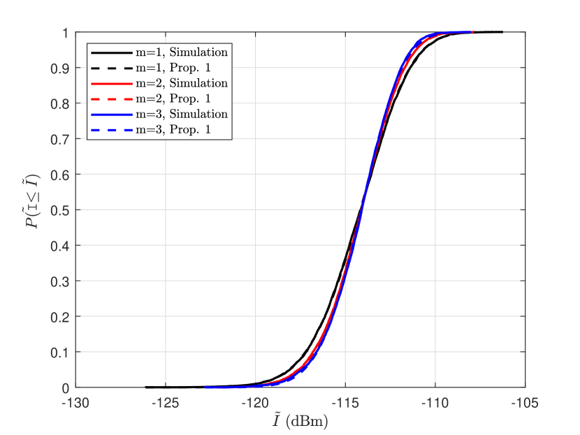
V-A Validity of Gamma Approximation
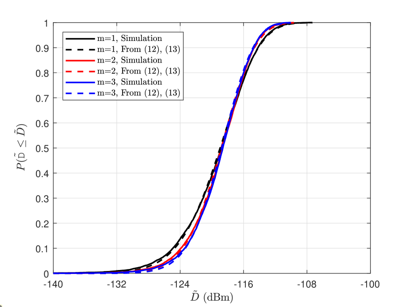
Figs. 2 and 3 show a comparison between the actual CDFs obtained from Monte Carlo simulations and our analytical CDFs. As can be seen in these figures, the Gamma random variables closely match the statistics of both and , which are defined on the state space of Poisson processes. Although the difference in CDFs is marginal, as will be shown in Figs. 4 and 5, gaps persist between the actual coverage probability and its lower and upper bounds. The deviation from actual results in CDFs can influence these gaps, in conjunction with the manipulation of the shape parameter. It is notable that, due to the small cluster area, Gamma approximation over involves fewer terms than because there are fewer satellites in the cluster area compared to those outside. Despite this, in Fig. 3, exhibits only a small deviation from the actual results, comparable to in Fig. 2.
V-B Derived Coverage Probability
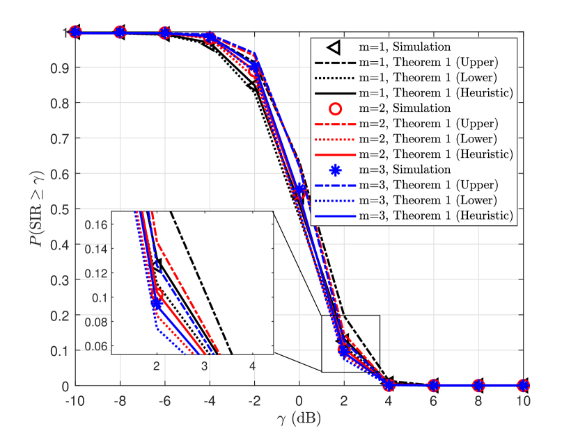
In Figs. 4 and 5, we plot the lower and upper bounds of the coverage probability based on and , in Scenarios 1 and 2, respectively. Additionally, we include a heuristic approach, denoted as , for comparison. This heuristic approach bridges the gap between the lower and upper bounds by linearly integrating them, incorporating weights determined by relative distance of with respect to and . The expression for the proposed heuristic approach is derived as:
| (32) | ||||
where the bounds of the coverage probability from Theorem 1 are applied. We can easily obtain the heuristic expression for the bounds obtained in Theorem 2 using the same principle. As the heuristic approach includes the effect of round processes by considering the weight, a close match with the actual result can be observed in both Figs. 4 and 5.
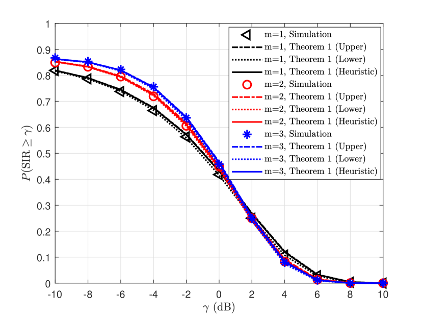
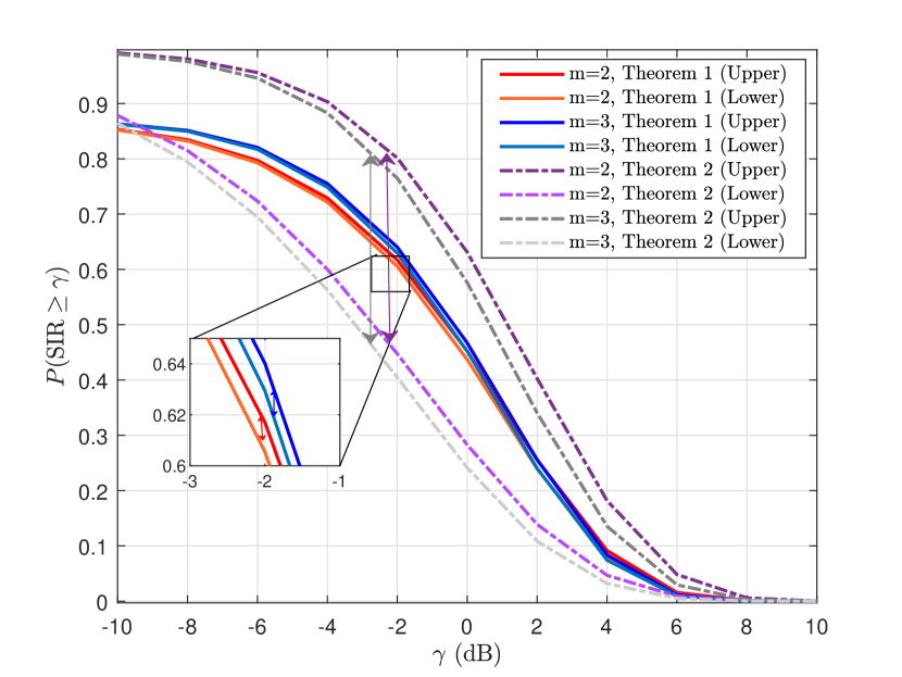
While both the lower and upper bounds effectively characterize the actual coverage probability, as shown in Fig. 6, the bounds derived from exhibit greater tightness than those obtained from . This difference in tightness arises from the larger shape parameter of compared to that of . As seen in (2), the shape parameter influences the number of operations. With an increase in operations, the gap between the lower and upper bounds narrows because the value of the final term becomes negligible. Consequently, the coverage probability bounds from with a high shape parameter are more refined than those from . However, there is a trade-off between the tightness and computational complexity, as a large shape parameter introduces an increased computational burden. Particularly in scenarios involving a massive number of satellites, the coverage probability bounds derived from can provide a fine bound while demanding significantly fewer computational resources. For instance, considering an average of satellites in the observable spherical dome with , the shape parameters for and are and , respectively. In this case, the coverage probability bounds utilizing can be computed within a manageable time frame, thanks to the smaller shape parameter.
V-C Impact of Cluster Area
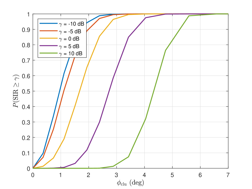
We investigate the impact of the cluster area, which is determined by , on the coverage probability. As increases, the cluster area expands, incorporating satellites that were previously causing interference into the cluster area for cooperative service to the user. Hence, the coverage probability is enhanced due to the increased accumulated cluster power and decreased accumulated interference power. Fig. 7 shows the coverage probabilities for various SIR thresholds and . As increases, the slope initially rises and then decreases beyond a specific for each SIR threshold. For example, with an SIR threshold dB, the coverage probability remarkably increases as rises from to but shows a slight increase from to . Additionally, for a given , we can determine the effective SIR threshold for a specific demanded coverage probability. For instance, if the cluster area is physically constrained to , setting the threshold to dB rather than dB is more efficient to enhance the network performance.
VI Conclusions
In this paper, we proposed the mathematical analyses of the performance of satellite cluster networks, where satellites in the cluster area collaborate to serve users, particularly in mega-constellations. To establish the lower and upper bounds of the coverage probability, we first derived the key parameters of the approximated Gamma random variables to handle the compound terms in the SIR and compared the advantages of each in terms of tightness and complexity. Leveraging the distribution of the approximated Gamma random variable, we suggested the lower and upper bounds of the coverage probability, which depend on system parameters. While the results in this work relied on random variable approximations and provided lower and upper bounds, these bounds effectively showed the network’s performance with sufficient tightness to simulation results. Moreover, our analyses not only reduced computational burden through finite operations but also expected to offer insights into the impact of system parameters on the coverage probability in satellite cluster networks.
Appendix A Proof of Proposition 1
For a Gamma random variable , its shape parameter and scale parameter are determined by the first and second-order moments and . By the Campbell’s theorem [38], the mean and the variance of the approximated Gamma random variable for the accumulated interference power are derived as follows
| (33) |
Appendix B Proof of Lemma 2
To derive the Laplace transform of the accumulated cluster power , we first derive the Laplace transform conditioned on , representing the condition that satellites are in the cluster area . The conditional Laplace transform of is given by
| (35) |
where (a) is obtained using the definition of and the Laplace transform, (b) follows from the conditional PDF given in Lemma 1, (c) results from the change of variable and the PDF for given in (5), and (d) uses the change of variable . The final expression in (2) is derived by using the definition of the Gamma function , which completes the proof.
Additionally, it is noteworthy that the conditional Laplace transform, considered in deriving the coverage probability, remains independent of the number of satellites . Taking the th root of (2), it becomes evident that the resulting th root of the conditional Laplace transform of is unaffected by the number of satellites .
Appendix C Proof of Theorem 1
The Erlang distribution is a special case of the Gamma distribution with a positive integer shape parameter. In the case of the Gamma random variable with the shape parameter , its lower and upper CDF bounds are represented using the Erlang distribution with the shape parameters (lower bound) and (upper bound) [15],[39]. The expression is as follows
| (36) |
In the same context, we transform the approximated Gamma distribution of the accumulated interference power to the Erlang distribution by round-up or -down the shape parameter to an integer .
To derive the lower and upper bounds of the coverage probability, the coverage probability with respect to is revisited
| (37) |
Invoking (36) into (37), we first derive the upper bound of the coverage probability with as
| (38) |
where (a) comes from the Erlang distribution with integer shape parameter , and (b) follows from the first derivative property of the Laplace transform . Replacing with , the lower bound of the coverage probability can be derived using the same process as in (C).
References
- [1] ITU, “Measuring the Information Society Report 2018,” vol. 2, pp. 3–4, Dec. 2018.
- [2] X. Chen, D. W. K. Ng, W. Yu, E. G. Larsson, N. Al-Dhahir, and R. Schober, “Massive Access for 5G and Beyond,” IEEE J. Sel. Areas Commun., vol. 39, no. 3, pp. 615–637, Mar. 2021.
- [3] S. Liu, Z. Gao, Y. Wu, D. W. Kwan Ng, X. Gao, K.-K. Wong, S. Chatzinotas, and B. Ottersten, “LEO Satellite Constellations for 5G and Beyond: How Will They Reshape Vertical Domains?” IEEE Commun. Mag., vol. 59, no. 7, pp. 30–36, Jul. 2021.
- [4] N. U. Hassan, C. Huang, C. Yuen, A. Ahmad, and Y. Zhang, “Dense Small Satellite Networks for Modern Terrestrial Communication Systems: Benefits, Infrastructure, and Technologies,” IEEE Wireless Commun., vol. 27, no. 5, pp. 96–103, Oct. 2020.
- [5] R. Wang, M. A. Kishk, and M.-S. Alouini, “Ultra-Dense LEO Satellite-Based Communication Systems: A Novel Modeling Technique,” IEEE Commun. Mag., vol. 60, no. 4, pp. 25–31, Apr. 2022.
- [6] I. del Portillo, B. G. Cameron, and E. F. Crawley, “A Technical Comparison of Three Low Earth Orbit Satellite Constellation Systems to Provide Global Broadband,” Acta Astronautica, vol. 159, pp. 123–135, Jun. 2019.
- [7] J. Yang, D. Li, X. Jiang, S. Chen, and L. Hanzo, “Enhancing the Resilience of Low Earth Orbit Remote Sensing Satellite Networks,” IEEE Netw., vol. 34, no. 4, pp. 304–311, Jul. 2020.
- [8] D.-H. Jung, G. Im, J.-G. Ryu, S. Park, H. Yu, and J. Choi, “Satellite Clustering for Non-Terrestrial Networks: Concept, Architectures, and Applications,” IEEE Veh. Technol. Mag., vol. 18, no. 3, pp. 29–37, Sept. 2023.
- [9] B. Al Homssi, A. Al-Hourani, K. Wang, P. Conder, S. Kandeepan, J. Choi, B. Allen, and B. Moores, “Next Generation Mega Satellite Networks for Access Equality: Opportunities, Challenges, and Performance,” IEEE Commun. Mag., vol. 60, no. 4, pp. 18–24, Apr. 2022.
- [10] M. Haenggi, Stochastic Geometry for Wireless Networks. Cambridge, England, U.K.: Cambridge University Press, 2012.
- [11] M. Haenggi, J. G. Andrews, F. Baccelli, O. Dousse, and M. Franceschetti, “Stochastic Geometry and Random Graphs for the Analysis and Design of Wireless Networks,” IEEE J. Sel. Areas Commun., vol. 27, no. 7, pp. 1029–1046, Sept. 2009.
- [12] J. G. Andrews, F. Baccelli, and R. K. Ganti, “A Tractable Approach to Coverage and Rate in Cellular Networks,” IEEE Trans. Commun., vol. 59, no. 11, pp. 3122–3134, Nov. 2011.
- [13] H. S. Dhillon, R. K. Ganti, F. Baccelli, and J. G. Andrews, “Modeling and Analysis of K-Tier Downlink Heterogeneous Cellular Networks,” IEEE J. Sel. Areas Commun., vol. 30, no. 3, pp. 550–560, Apr. 2012.
- [14] T. D. Novlan, H. S. Dhillon, and J. G. Andrews, “Analytical Modeling of Uplink Cellular Networks,” IEEE Trans. Wireless Commun., vol. 12, no. 6, pp. 2669–2679, Jun. 2013.
- [15] R. Tanbourgi, S. Singh, J. G. Andrews, and F. K. Jondral, “A Tractable Model for Noncoherent Joint-Transmission Base Station Cooperation,” IEEE Trans. Wireless Commun., vol. 13, no. 9, pp. 4959–4973, Sept. 2014.
- [16] M. Afshang and H. S. Dhillon, “Fundamentals of Modeling Finite Wireless Networks Using Binomial Point Process,” IEEE Trans. Wireless Commun., vol. 16, no. 5, pp. 3355–3370, May 2017.
- [17] N. Okati, T. Riihonen, D. Korpi, I. Angervuori, and R. Wichman, “Downlink Coverage and Rate Analysis of Low Earth Orbit Satellite Constellations Using Stochastic Geometry,” IEEE Trans. Commun., vol. 68, no. 8, pp. 5120–5134, Aug. 2020.
- [18] D.-H. Jung, J.-G. Ryu, W.-J. Byun, and J. Choi, “Performance Analysis of Satellite Communication System Under the Shadowed-Rician Fading: A Stochastic Geometry Approach,” IEEE Trans. Commun., vol. 70, no. 4, pp. 2707–2721, Apr. 2022.
- [19] A. Talgat, M. A. Kishk, and M.-S. Alouini, “Stochastic Geometry-Based Analysis of LEO Satellite Communication Systems,” IEEE Commun. Lett., vol. 25, no. 8, pp. 2458–2462, Aug. 2021.
- [20] J. Park, J. Choi, and N. Lee, “A Tractable Approach to Coverage Analysis in Downlink Satellite Networks,” IEEE Trans. Wireless Commun., vol. 22, no. 2, pp. 793–807, Feb. 2023.
- [21] A. Al-Hourani, “An Analytic Approach for Modeling the Coverage Performance of Dense Satellite Networks,” IEEE Wireless Commun. Lett., vol. 10, no. 4, pp. 897–901, Apr. 2021.
- [22] ——, “Optimal Satellite Constellation Altitude for Maximal Coverage,” IEEE Wireless Commun. Lett., vol. 10, no. 7, pp. 1444–1448, Jul. 2021.
- [23] N. Okati and T. Riihonen, “Nonhomogeneous Stochastic Geometry Analysis of Massive LEO Communication Constellations,” IEEE Trans. Commun., vol. 70, no. 3, pp. 1848–1860, Mar. 2022.
- [24] J. Lee, S. Noh, S. Jeong, and N. Lee, “Coverage Analysis of LEO Satellite Downlink Networks: Orbit Geometry Dependent Approach,” arXiv:2206.09382v1, Jun. 2022.
- [25] C.-S. Choi and F. Baccelli, “A Novel Analytical Model for LEO Satellite Constellations Leveraging Cox Point Processes,” arXiv:2212.03549v3, Dec. 2023.
- [26] H. M. Cundy and A. P. Rollett, Mathematical Models, 3rd ed. Stradbroke, England, U.K.: Tarquin Publications, 1981.
- [27] J. Tang, D. Bian, G. Li, J. Hu, and J. Cheng, “Resource Allocation for LEO Beam-Hopping Satellites in a Spectrum Sharing Scenario,” IEEE Access, vol. 9, pp. 56 468–56 478, 2021.
- [28] A. Koretz and B. Rafaely, “Dolph–Chebyshev Beampattern Design for Spherical Arrays,” IEEE Trans. Signal Process., vol. 57, no. 6, pp. 2417–2420, Jun. 2009.
- [29] T. Bai and R. W. Heath, “Coverage and Rate Analysis for Millimeter-Wave Cellular Networks,” IEEE Trans. Wireless Commun., vol. 14, no. 2, pp. 1100–1114, Feb. 2015.
- [30] S. Singh, M. N. Kulkarni, A. Ghosh, and J. G. Andrews, “Tractable Model for Rate in Self-Backhauled Millimeter Wave Cellular Networks,” IEEE J. Sel. Areas Commun., vol. 33, no. 10, pp. 2196–2211, Oct. 2015.
- [31] M. Di Renzo, “Stochastic Geometry Modeling and Analysis of Multi-Tier Millimeter Wave Cellular Networks,” IEEE Trans. Wireless Commun., vol. 14, no. 9, pp. 5038–5057, Sept. 2015.
- [32] M. Haenggi and R. Ganti, Interference in Large Wireless Networks. NOW: Foundations and Trends in Networking, 2009.
- [33] R. W. Heath, M. Kountouris, and T. Bai, “Modeling Heterogeneous Network Interference Using Poisson Point Processes,” IEEE Trans. Signal Process., vol. 61, no. 16, pp. 4114–4126, Aug. 2013.
- [34] S. N. Chiu, D. Stoyan, W. S. Kendall, and J. Mecke, Stochastic Geometry and Its Applications. Hoboken, NJ, USA: Wiley, 2013, vol. 3.
- [35] I. S. Gradshteyn and I. M. Ryzhik, Table of Integrals, Series, and Products. New York, NY, USA : Academic, 2014.
- [36] N. T. Thomopoulos, Statistical Distributions: Applications and Parameter Estimates. Cham: Cham, Switzerland: Springer International Publishing, 2017.
- [37] E. T. Bell, “Exponential Polynomials,” Ann. Math, vol. 35, pp. 258–277, 1934.
- [38] J. F. C. Kingman, Poisson processes. Oxford, England, U.K.: Clarendon Press, 1992, vol. 3.
- [39] G. Karagiannidis, N. Sagias, and T. Tsiftsis, “Closed-Form Statistics for The Sum of Squared Nakagami-m Variates and Its Applications,” IEEE Trans. Commun., vol. 54, no. 8, pp. 1353–1359, Aug. 2006.