Referee Can Play: An Alternative Approach to Conditional Generation via Model Inversion

Abstract

As a dominant force in text-to-image generation tasks, Diffusion Probabilistic Models (DPMs) face a critical challenge in controllability, struggling to adhere strictly to complex, multi-faceted instructions. In this work, we aim to address this alignment challenge for conditional generation tasks. First, we provide an alternative view of state-of-the-art DPMs as a way of inverting advanced Vision-Language Models (VLMs). With this formulation, we naturally propose a training-free approach that bypasses the conventional sampling process associated with DPMs. By directly optimizing images with the supervision of discriminative VLMs, the proposed method can potentially achieve a better text-image alignment. As proof of concept, we demonstrate the pipeline with the pre-trained BLIP-2 model and identify several key designs for improved image generation. To further enhance the image fidelity, a Score Distillation Sampling module of Stable Diffusion is incorporated. By carefully balancing the two components during optimization, our method can produce high-quality images with near state-of-the-art performance on T2I-Compbench.

Figure 6: Our method can effectively generate faithful images strictly following the prompt “Two hot dogs sit on a white paper plate near a soda cup which is sitting on a green picnic table while a bike and a silver car are parked nearby”. However, the baseline methods, including Stable Diffusion (SD) 1.5, Attend-and-Excite (Chefer et al., 2023), PixArt-$\alpha$ (Chen et al., 2023a), DALLE-2 (OpenAI, 2023), DALLE-3 (Betker et al., 2023), struggle to generate the right images encountering this kind of complex compositional prompts.

1 Introduction

With exceptional sample quality and scalability, DPMs (Sohl-Dickstein et al., 2015; Ho et al., 2020; Song et al., 2020) have significantly contributed to the success of Artificial Intelligence Generated Content (AIGC), especially in text-to-image generation. The performance of state-of-the-art (SOTA) DPMs, e.g., Stable Diffusion (Rombach et al., 2022; Podell et al., 2023), PixArt-$\alpha$ (Chen et al., 2023a), in generating various images with high-fidelity is no longer a major concern. What is left to be desired is controllability, i.e., the compatibility between the generated image and the input text. For instance, a simple composite prompt like “a red backpack and a blue book” is challenging for Stable Diffusions (SD) (Huang et al., 2023).

To better understand the condition injection mechanism of modern text-to-image generation models, let us first consider the relationship between text (i.e., condition) and image. In practice, the actual condition the model takes usually contains an extended version of the input prompt paraphrased by language models. As the text description gets richer, more information is dictated for the target image with less nuisance to fill. In other words, the stochasticity of the generation task gradually decreases with extra conditions, where we may even expect almost one-to-one matching between the text and image. This transition calls for new thinking about the conditional generation task.

On the one hand, when training such strong-condition models, high-quality paired data $(\mathbf{x},\mathbf{y})$ are needed where $\mathbf{x}$ satisfies the condition $\mathbf{y}$. For most of the generative models, the generation process can be described as mapping $(\mathbf{y},\mathbf{\epsilon})$ to $\mathbf{x}$ where $\mathbf{\epsilon}$ is a random vector providing diversity. In practice, the controllability of the generative model is critically dependent on the label quality, i.e., $\mathbf{y}|\mathbf{x}$ should be as detailed as possible. Beyond human labeling, SOTA DPMs such as DALLE-3 (Betker et al., 2023) utilize powerful vision language models (VLMs) to regenerate image captions during training. Then, given a new prompt $\mathbf{y}$ at the inference phase, the ideal image $\mathbf{x}|\mathbf{y}$ should be deemed fit by the VLM. From this perspective, the text-to-image generation case can be seen as a model inversion task on the VLM, with explicit mappings parametrized by the score network in DPMs. On the other hand, the discriminative module also plays a more central role in aligning with the condition. As supporting evidence, consider the importance of guidance in current text-to-image DPMs (Ho & Salimans, 2022; Bansal et al., 2023; Ma et al., 2023). Although designed to work directly, a relatively large classifier-free guidance (CFG) coefficient is indispensable (7.5 by default in SD). When faced with the strong condition of a multi-attribute object correspondence, the image produced by a higher CFG is more semantically compliant (see results in Appendix A.1).

The utilization of VLM in DALLE-3 and a higher CFG in SD emphasize the importance of the discriminative component for image-text alignment, which may have been overshadowed by the generative counterpart. Fortunately, discrimination (image-to-text) is relatively easier than generation (text-to-image), since an image often contains more information than its text description. When a misalignment happens during diffusion generation, it can be trivial for a VLM to tell. Based on this premise, T2I-CompBench (Huang et al., 2023) employs several discriminative VLMs, e.g., BLIP-VQA (Li et al., 2022) and CLIP (Radford et al., 2021) as referees, to measure text-image compatibility of SOTA generative models. The alignment can be further improved by finetuning with “good” text-image data selected by the referees.

Inspired by the above observations, we propose a novel conditional image generation paradigm predominantly led by VLMs for improved image-text alignment. Given textual prompts, we generate images by conducting model inversion on the VLM. Specifically, we keep the VLM parameters fixed, treating the image as the optimization object. For more efficient parameterization, we adopt the pre-trained VAE used in the latent diffusion model (Rombach et al., 2022) and conduct optimization on the latent variable space $\mathbf{z}$. We start with random noise and progressively refine $\mathbf{z}$ by minimizing the loss function used in VLM pre-training, which measures image-text consistency (Figure 7 illustrates the core idea of our method and its comparison against current DPMs). Additionally, to enhance image fidelity, we propose incorporating gradients provided by Score Distillation Sampling. The overall generation pipeline is entirely training-free and data-free, and the controllability of our method is greatly improved compared to SD. While our method may not generate images as elaborate as those specialized generation models like DALLE-3, we achieve comparable performance on image-text alignment.

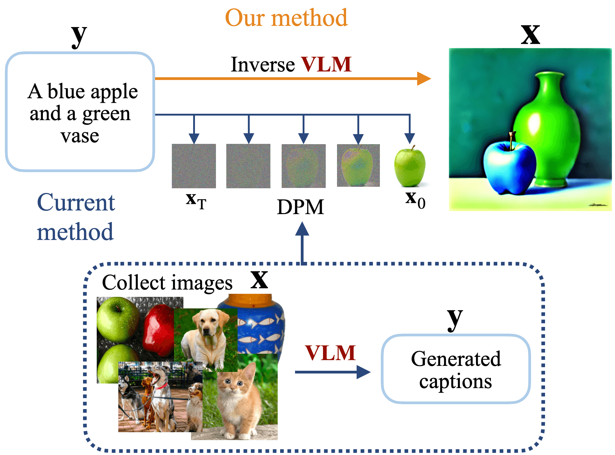
Figure 7: SOTA image generation models require collecting a large number of images which are then labeled in detail by a VLM for training. During the inference phase, the condition ($\mathbf{y}$) is injected into the denoising process of random noise ($\mathbf{x}_{\mathrm{T}}$) through a cross-attention mechanism. The key difference in our approach is that we generate images by directly inversing the VLM, eliminating the need to train a specialized generation model.

The main contributions of this work are summarized below.

• We introduce a novel perspective by understanding strong conditional text-to-image generation as model inversion, shedding light on the crucial role of discriminative models in the conditional generation process.

• We propose a method that places discriminative models such as VLMs at the forefront, introducing a shift in the text-to-image generation paradigm. Our method is training-free and highly flexible. Several key design choices are elucidated, e.g., augmentation regularization, exponential moving average with restart, etc.

• Our method achieves near SOTA results on benchmarks that measure the generation models’ controllability (Huang et al., 2023).

2 Preliminary

Discriminative Vision Language Models

VLMs represent a pivotal advancement in the field of multimodal representation learning. These models undergo extensive pre-training on expansive datasets comprising image-text pairs, enabling them the capacity for zero-shot predictions across a diverse spectrum of tasks that encompass both visual and linguistic information, including image-text retrieval, image captioning, visual question answering (VQA), etc (Du et al., 2022). The central objective of VLM pre-training is to imbue these models with a profound understanding of the intricate alignment between textual and visual modalities. To achieve this goal, various alignment losses are employed, e.g., contrastive loss in CLIP (Radford et al., 2021), ALIGN (Jia et al., 2021), ALBEF (Li et al., 2021), BLIP (Li et al., 2022), BLIP -2(Li et al., 2023a). In contrast to text-to-image generation models, VLMs exhibit a superior aptitude for aligning textual and visual information. CLIP image-text similarity is widely utilized to measure the alignment of the generated images with the textual condition (Hessel et al., 2021; Ma et al., 2023). A recent compositional text-to-image generation evaluation benchmark T2I-CompBench (Huang et al., 2023) further uses the BLIP-VQA model (Li et al., 2022) as a referee to judge the correctness of the generated images.

Latent Diffusion Models

Latent diffusion models (LDMs) (Rombach et al., 2022) conduct the forward and reverse processes in the latent space of an autoencoder. The additional encoder $\mathrm{ENC}$ and decoder $\mathrm{DEC}$ are required to map the original image $\mathbf{x}$ to a latent variable $\mathbf{z}$ and reconstruct the image from $\mathbf{z}$, such that $\mathrm{DEC}(\mathrm{ENC}(\mathbf{x}))\approx\mathbf{x}$. Classifier-free guidance (CFG) (Ho & Salimans, 2022) is a commonly used conditional generation method in DPMs. Given a condition $\mathbf{y}$ and a pre-trained text-to-image DPM with the noise prediction neural network $\phi$, CFG generates images via $\widehat{\epsilon}(\mathbf{x}_{t};\mathbf{y},t)=\epsilon_{\phi}(\mathbf{x}_{t};\mathbf{y},t)+s(\epsilon_{\phi}(\mathbf{x}_{t};\mathbf{y},t)-\epsilon_{\phi}(\mathbf{x}_{t};t)$), where $s>0$ is the guidance scale.

Score Distillation

Score distillation sampling (SDS) is an optimization mechanism to distill the rich knowledge from pre-trained text-to-image generation diffusion models (Poole et al., 2022; Luo et al., 2023). SDS allows optimizing differentiable generators, and it has been widely explored in text-to-3D generation (Wang et al., 2023c, a), and image editing tasks (Hertz et al., 2023; Kim et al., 2023a). Given a pre-trained text-to-image LDM with the noise prediction neural network $\phi$ with noise $\epsilon\sim\mathcal{N}(\mathbf{0},\mathbf{1})$, SDS optimizes a group of parameters $\theta$ by:

$$\nabla_{\theta}\mathcal{L}_{SDS}(\phi,\mathbf{x}=g(\theta))\approx\mathbb{E}_{t,\mathbf{\epsilon}}[(\mathbf{\epsilon_{\phi}}(\mathbf{z}_{t};\mathbf{y},t)-\mathbf{\epsilon})\frac{\partial\mathbf{x}}{\partial\theta}],$$

where $g(\theta)$ can be any differentiable function.

3 Conditional generation via model inversion

The image caption quality is critical for training text-to-image generation models that possess good image-text understanding ability. State-of-the-art models have increasingly harnessed discriminative VLMs’ capabilities to improve the controllability and precision of image synthesis, such as DALLE-3 (Betker et al., 2023) and PixArt-$\alpha$ (Chen et al., 2023a). By generating comprehensive and detailed textual descriptions for images ($\mathbf{x}\stackrel{{\scriptstyle\mathrm{VLM}}}{{\longrightarrow}}\mathbf{y}$), the gap between textual and visual information narrows down, allowing the image generation model (e.g., DPMs) to master a more exact alignment. At the inference stage, the model is required to generate images from the provided prompt ($\mathbf{y}\stackrel{{\scriptstyle\mathrm{DPM}}}{{\longrightarrow}}\mathbf{x}$). Therefore, the diffusion model essentially functions as a learned inverse of the VLM.

Instead of training a DPM to learn the inverse function of VLM, we venture into directly leveraging VLM to perform the reverse task: generating the corresponding image given a text prompt via optimization. From the perspective of model inversion, the inverse map learned by mainstream DPMs is parameterized by the score net and can be thought of as continuous (it’s a deterministic map if using ODE sampler). In clear contrast, the inverse map from direct optimization-based model inversion is stochastic and not continuous. Thanks to the discontinuity, the inverse map from the latter approach is not limited by any neural network parameterization and can be unlimited in terms of expressivity (Feng et al., 2021; Hu et al., 2023).

3.1 Vision Language Model Inversion for Alignment

To fully harness the text and image alignment information ingrained within the pre-trained VLMs, we propose to synthesize text-conditional images commencing from random noise with the supervision of a VLM.

Problem formulation

Denote the alignment loss given by a VLM as $L(\mathbf{x},\mathbf{y})$, where a smaller $L(\mathbf{x},\mathbf{y})$ indicates better alignment between $\mathbf{x}$ and $\mathbf{y}$. We formulate the conditional generation task as an optimization problem, i.e., $\min_{\mathbf{x}}L(\mathbf{x},\mathbf{y})$, where the VLM is kept frozen, and the image is the optimizing target. No extra training or data is needed, so our method is highly efficient. As a proof of concept, we demonstrate with the pre-trained BLIP-2 (Li et al., 2023a) model, which has lightweight training loss and good zero-shot performance. We utilize the image-text matching loss $L_{itm}$ and the caption generation loss $L_{cg}$ in BLIP-2 pre-training (Li et al., 2021), i.e., $L(\mathbf{x},\mathbf{y})=L_{itm}+L_{cg}$.

Parameterization

Images usually reside in high-dimensional spaces (e.g., $512\times 512\times 3$), which makes the optimization problem challenging and computationally expensive. Inspired by LDMs (Rombach et al., 2022), we utilize a pre-trained autoencoder to reduce the dimensionality of the optimization target from pixel space to low-dimensional latent space. We choose the widely used KL-VAE with a downsampling factor $f=8$ in the LDM (Rombach et al., 2022). Denote the decoder as $\mathrm{DEC}$. Then, $\mathbf{x}$ is parameterized as $\mathrm{DEC}(\mathbf{z})$ and we can directly work with $\mathbf{z}\in\mathbb{R}^{64\times 64\times 4}$.

Necessity of Regularization

Achieving high-quality images through direct discriminative model inversion is almost impossible (Yin et al., 2020; Wang & Torr, 2022). The first row of Figure 8 shows the generated images from a naive implementation of the above proposal. During optimization, the alignment loss can be effectively minimized, but the resulting images are not natural. They can be thought of as adversarial samples that are recognized by VLMs but not humans. The existence of adversarial samples has been extensively studied in the adversarial robustness literature (Goodfellow et al., 2014; Arrieta et al., 2020). Therefore, generating plausible images by vanilla optimization is not viable. Extra regularization is needed to constrain the search space to align with human perception.

To address the challenge, we take inspiration from contrastive learning, where semantic invariant augmentations are constructed to specify the equivariant groups in the feature space so that learning can be more efficient (Dangovski et al., 2021; HaoChen & Ma, 2022; Hu et al., 2022). Similarly, we consider generating multiple samples with semantic invariance but slight image variations through data augmentation $A\sim\mathbb{P}_{A}$ and use their averaged loss as the optimization objective. Correspondingly, we can define the augmentation-regularized loss as

$$\widetilde{L}_{\mathbf{y}}(\mathbf{x}):=\mathbb{E}_{A}L(A(\mathbf{x}),\mathbf{y}),$$ (1)

where the expectation is taken over the random augmentations. This is similar to random smoothing (Cohen et al., 2019; Li et al., 2019; Ding et al., 2023). The augmentation regularizes the search space by removing the adversarial solutions $\mathbf{x}$ where $L(\mathbf{x})$ is low while $\widetilde{L}(\mathbf{x})$ is high. To illustrate, consider $\mathbb{P}_{A}$ as random masking. Then, for any specific masking $A^{\prime}$, $\widetilde{L}_{\mathbf{y}}(\mathbf{x})\leq c$ implies that

$$\widetilde{L}_{\mathbf{y}}(A^{\prime}(\mathbf{x}))\leq c+\mathbb{P}(A\notin S_{A^{\prime}})\cdot$$

$$\mathbb{E}_{A\notin S_{A^{\prime}}}\left[L_{\mathbf{y}}((A\circ A^{\prime})(\mathbf{x}))-L_{\mathbf{y}}(A(\mathbf{x}))\right],$$

where $S_{A^{\prime}}=\{A\mid A\circ A^{\prime}=A\}$. Thus, minimizing $\widetilde{L}(\mathbf{x})$ implicitly minimizes $\widetilde{L}(A^{\prime}(\mathbf{x}))$ for all $A^{\prime}$ such that $\mathbb{P}(A\notin S_{A^{\prime}})$ is low. To verify, an image $\mathbf{x}$ in the 1st row of Figure 8 indeed obtains a low $L(\mathbf{x})$, while having a high $\widetilde{L}(\mathbf{x})$ (see results in Table 2). Thus, such an adversarial solution is removed in the 2nd and 3rd rows where a returned image $\mathbf{x}$ is ensured to have low values in $\widetilde{L}$. This augmentation regularization has been proven effective in improving overall results, including the perceptual image quality (Figure 8) and BLIP-VQA score (Table 1).

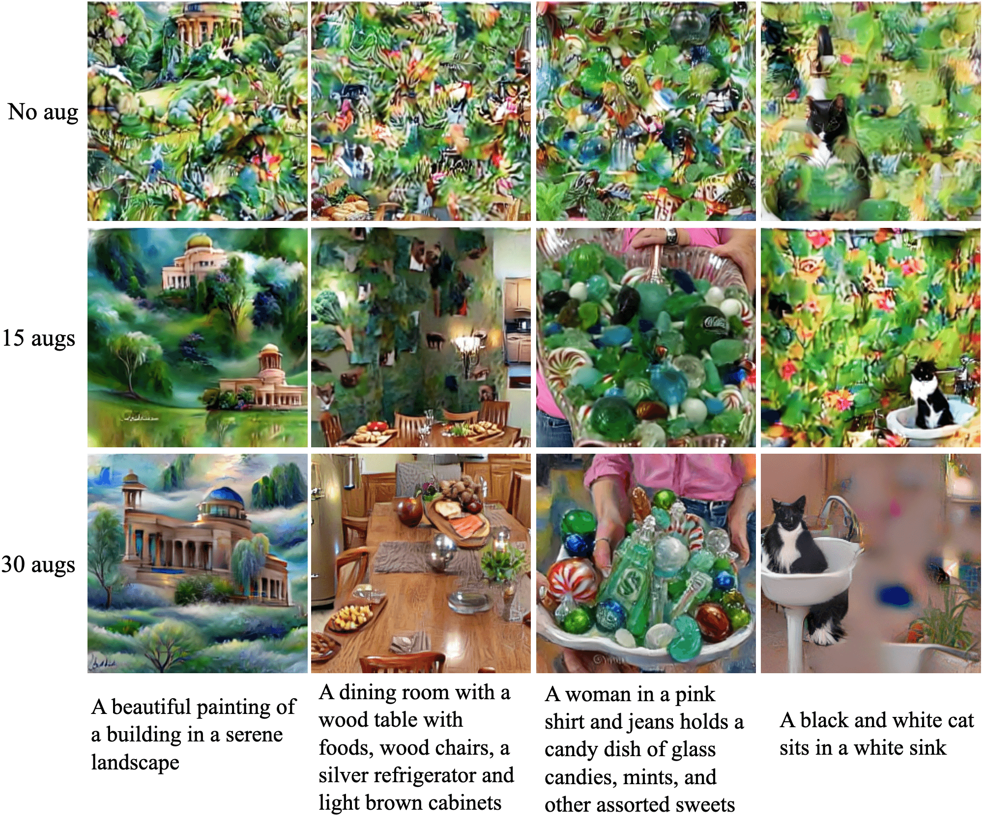
Figure 8: The illustration of the influence of augmentation regularization on BLIP-2 inversion. We show the result of no augmentation (top row), 15 augmentations (middle row), and 30 augmentations (bottom row).

Table 1: The BLIP-VQA score of BLIP-2 inversion without and with augmentations on Attribute-binding dataset

	color	shape	texture
no aug	0.6561	0.5078	0.5371
30 augs	0.8639	0.6686	0.7311

Table 2: The average BLIP-2 loss ($L_{itm}\&L_{cg})$ of images on the 1st and 3rd row of Figure 8.

	$L(\mathbf{x})$	$\widetilde{L}(\mathbf{x})$
no aug (1st row)	2e-3 $\&$ 3.28	5.65 $\&$ 4.66
30 augs (3rd row)	1e-5 $\&$ 3.08	2e-3 $\&$ 3.30

As an added benefit, augmentation regularization contributes to smoother images and lower loss values, as can be seen in Table 2. The following propositions unveil that Gaussian random augmentation will result in a smoother objective function and easier optimization for model inversion. All technical details can be found in Appendix B.

Proposition 3.1 (informal).

Under some mild regularity conditions on the augmentation, $\widetilde{L}_{y}$ is strictly smoother than $L_{y}$. Particularly, if $A(\mathbf{x})=\mathbf{x}+\epsilon$ where $\epsilon$ is Gaussian, $\widetilde{L}_{y}$ has infinite smoothness and is Lipschitz continuous.

The optimization problem can greatly benefit from both a smoother objective function (Kovalev & Gasnikov, 2022) and bounded Lipschitz constant (Ghadimi & Lan, 2013; Bertsekas, 2016). From another angle, augmentation can also improve the condition number of convex optimization, as stated in the following proposition.

Proposition 3.2 (informal).

Assume $L_{c}(\cdot)$ is a convex function and denote its Hessian matrix at $x$ as $\partial^{2}L_{c}(x)$. Under some mild regularity conditions, the condition number of $\partial^{2}\widetilde{L}_{c}$ is strictly smaller than that of $\partial^{2}L_{c}(x)$.

Ideal Augmentations for BLIP-2 Inversion

Our proposed BLIP-2 inversion posts new requirements for the ideal augmentations. We have conducted extensive ablation experiments to identify suitable augmentation techniques from conservative learning. Eventually, we employ random affine, random perspective, color-jitter, random erasing, and Gaussian noise and discard horizontal flipping and random cropping, due to a notable adverse impact on the final image (detailed results in Appendix A.3). This is to be expected since, in our case, the considered semantic information is much more intricate than that in contrastive learning. For instance, some captions may contain “left” or “right” location information, which will be significantly altered by horizontal flipping. The ineffectiveness of these augmentations is also reflected in the BLIP-2 loss. Within the same batch of augmented images, horizontal flipping and random cropping result in larger loss values. Such issues related to data augmentation altering semantics have been widely studied in the context of contrastive learning (Chen et al., 2020; Tian et al., 2020; Kalantidis et al., 2020; Patrick et al., 2021; Chuang et al., 2022).

In conclusion, with the aforementioned formulation and augmentation regularization, VLMs can be effectively inversed to generate images with both good visual quality and high alignment to given prompts. Table 3 (“BLIP-2 INV”) demonstrates SOTA alignment score on Attribute-binding dataset (Huang et al., 2023). However, since the pre-training of BLIP-2 is primarily a discriminative task, it is inevitable that a significant amount of image information is lost during its forward pass, making it challenging to recover this information through model inversion. Additional help is required to achieve a high aesthetic quality.

3.2 SDS for Improved Fidelity

To make our generated images more realistic, integrating the gradient provided by another model focusing on image fidelity can help. A natural choice is Score Distillation Sampling (SDS), an optimization method based on knowledge distillation (Poole et al., 2022) that has shown great ability in generating or editing images. We first investigate the effectiveness of SDS as a standalone image generator and measure its performance in image-text matching. Additionally, we thoroughly explore how SDS can aid model inversion in generating controllable and plausible images.

3.3 Delicate Balance

Our method consists of two modules, with VLM taking the lead in generating condition-compliant images and SDS ensuring the fidelity and aesthetics of the images. Integrating them is not a straightforward task. In our experiments, we observe that these two components tend to prioritize different aspects and may result in divergent optimization directions. BLIP-2 inversion is primarily concerned with semantic alignment, whereas SDS prioritizes image fidelity. SDS often misinterprets prompts, resulting in images with missing objects or misaligned attributes when dealing with compositional prompts. In contrast, BLIP-2 inversion is far superior in following the instructions. The image evolution processes of two modules individually clearly illustrate these phenomena (see Figure 30 and 31 in Appendix A.5). Consequently, when BLIP-2 inversion and SDS collaborate, the gradients provided by these two modules reflect different objectives (examples shown in Appendix A.5 Figure 33). This issue calls for carefully tuning the individual weights, which we discuss and demonstrate with results in the experiment section.

Algorithm 1 Conditional Generation via VLM Inverion and SDS

  Input: A text prompt $\mathbf{y}$,

  Required: a pre-trained VLM model (e.g., BLIP2) and the loss function $L$, a pre-trained Stable Diffusion model $\phi$, and a decoder $\mathrm{DEC}$.

  Output: Generated image $\mathbf{x}$ following $\mathbf{y}$.

  Set augmentation function $A$, learning rate $\beta$, weight $w_{1}$ for BLIP-2 and weight $w_{2}$ for SDS; EMA decay rate $\lambda$, EMA start iteration $e_{s}$ and EMA restart iteration $e_{rs}$.

  Initialize $\mathbf{z}_{0}\leftarrow$ sample from $\mathcal{N}(\mathbf{0},\mathbf{I})$; $\mathbf{z}_{0}^{ema}=\mathbf{z}_{0}$

  for $i=1$ to $I$ do

     $\mathbf{x}_{i}=\mathrm{DEC}(\mathbf{z}_{i-1})$

     $\nabla_{\mathbf{z}}^{{}^{\prime}}\mathcal{L}_{SDS}(\phi,\mathbf{z}_{i-1},\mathbf{y})=w_{2}\nabla_{\mathbf{z}}\mathcal{L}_{SDS}(\phi,\mathbf{z}_{i-1},\mathbf{y})$

     $\nabla_{\mathbf{z}}^{{}^{\prime}}\widetilde{L}_{\mathbf{y}}(\mathbf{x}_{i})$ = $w_{1}\nabla_{\mathbf{z}}\widetilde{L}_{\mathbf{y}}(\mathbf{x}_{i})$ $\cdot$ $\frac{||\nabla_{\mathbf{z}}\mathcal{L}_{SDS}(\phi,\mathbf{z}_{i-1},\mathbf{y})||}{||\nabla_{\mathbf{z}}\widetilde{L}_{\mathbf{y}}(\mathbf{x}_{i})||}$

     $\mathbf{z}_{i}$ $\leftarrow$ Adam($\mathbf{z}_{i-1}$, $\beta$, $\nabla_{\mathbf{z}}^{{}^{\prime}}\widetilde{L}_{\mathbf{y}}(\mathbf{x}_{i})$)

     $\mathbf{z}_{i}$ $\leftarrow$ $\mathbf{z}_{i}-\beta$ $\nabla_{\mathbf{z}}^{{}^{\prime}}\mathcal{L}_{SDS}(\phi,\mathbf{z}_{i-1},\mathbf{y})$

     $\mathbf{z}_{i}^{ema}\leftarrow\lambda$ $\mathbf{z}_{i-1}^{ema}$ + $(1-\lambda)$ $\mathbf{z}_{i}^{ema}$

     if $i\geq e_{s}$ and $(i-e_{s})\%e_{rs}=0$ then

        $\mathbf{z}_{i}\leftarrow\mathbf{z}_{i}^{ema}$

     end if

  end for

  $\mathbf{x}=\mathrm{DEC}(\mathbf{z})$

  return $\mathbf{x}$

Exponential moving average (EMA) restart strategy is further proposed to enhance the stability of the two modules’ collaboration. EMA has been widely used in deep network optimization that includes two modules or branches (Tarvainen & Valpola, 2017; He et al., 2020; Cai et al., 2021), showing the strength to provide stable optimization and improved prediction. Unlike the conventional EMA method, EMA-restart involves replacing the original optimization target with its EMA version at a specified iteration location. Two extra hyperparameters are involved in EMA-restart: starting with the start iteration location, the parameters are replaced by their EMA versions, and then every other time after the restart interval. Appropriate use of EMA-restart can effectively enhance stability during the optimization process and improve the image-text matching degree.

The overall algorithm is depicted in Algorithm 1.

4 Experiments

Implementation details can be found in Appendix C. We mainly represent the experiment results, analysis, and ablation studies in this section.

Table 3: Image-text alignment evaluation on T2I-CompBench. The best results are marked in green, and the second best in blue. The baseline data are sourced from (Chen et al., 2023a).

Model	Attribute Binding			Object Relationship		Complex
	Color $\uparrow$	Shape $\uparrow$	Texture $\uparrow$	Spatial $\uparrow$	Non-spatial $\uparrow$
Stable v1.4	0.3765	0.3576	0.4156	0.1246	0.3079	0.3080
Composable v2	0.4063	0.3299	0.3644	0.0800	0.2980	0.2898
Structured v2	0.4990	0.4218	0.4900	0.1386	0.3111	0.3355
Attn-Exct v2	0.6400	0.4517	0.5963	0.1455	0.3199	0.3401
GORS	0.6603	0.4785	0.6287	0.1815	0.3193	0.3328
DALLE-2	0.5750	0.5464	0.6374	0.1283	0.3043	0.3696
SDXL	0.6369	0.5408	0.5637	0.2032	0.3110	0.4091
PixART-$\alpha$	0.6886	0.5582	0.7044	0.2082	0.3179	0.4117
DALLE-3	0.8110	0.6750	0.8070	-	-	-
SDS v1.5	0.3793	0.3914	0.4321	0.1261	0.3038	0.2773
BLIP-2 Inv	0.8639	0.6686	0.7311	0.1008	0.3260	0.3379
our method	0.8162	0.6209	0.7202	0.1506	0.3215	0.3529

SD v1-5

Struc-Diff

Attn-Exct

Our method

Figure 24: Qualitative Comparison using prompts from Attribute-binding of T2I-CompBench (Huang et al., 2023). We generate two images for each prompt with the same two random seeds for all methods.

Table 4: Results with different EMA start iterations $e_{s}$ and restart intervals $e_{rs}$. Baseline results include without EMA: 67.43 (75.76/48.36/78.71); with original EMA: 67.22 (76.98/47.36/77.32).

$e_{rs}$\ $e_{s}$	20	40	60	80
10	65.49 (76.86/46.25/73.35)	67.75 (77.24/49.52/76.50)	65.89 (75.18/47.06/75.41)	67.15 (78.10/45.19/78.16)
20	67.96 (81.70/49.91/72.27)	65.76 (77.06/43.04/72.18)	62.61 (73.00/46.68/78.14)	71.77 (79.47/50.56/85.29)
40	64.55 (72.53/48.51/77.61)	65.11 (69.89/48.77/76.68)	71.86 (80.36/49.06/86.16)	66.73 (76.20/38.20/75.99)
60	71.24 (68.90/50.43/84.40)	72.47 (83.99/53.41/80.01)	67.14 (78.52/46.39/76.50)	66.73 (76.20/38.20/75.99)

4.1 Quantitative Results

We evaluate our method on T2I-CompBench (Huang et al., 2023), a comprehensive benchmark for open-world compositional text-to-image generation consisting of attribute binding, object relationships, and complex compositions. The results are presented in Table 3.

4.2 Qualitative Comparisons

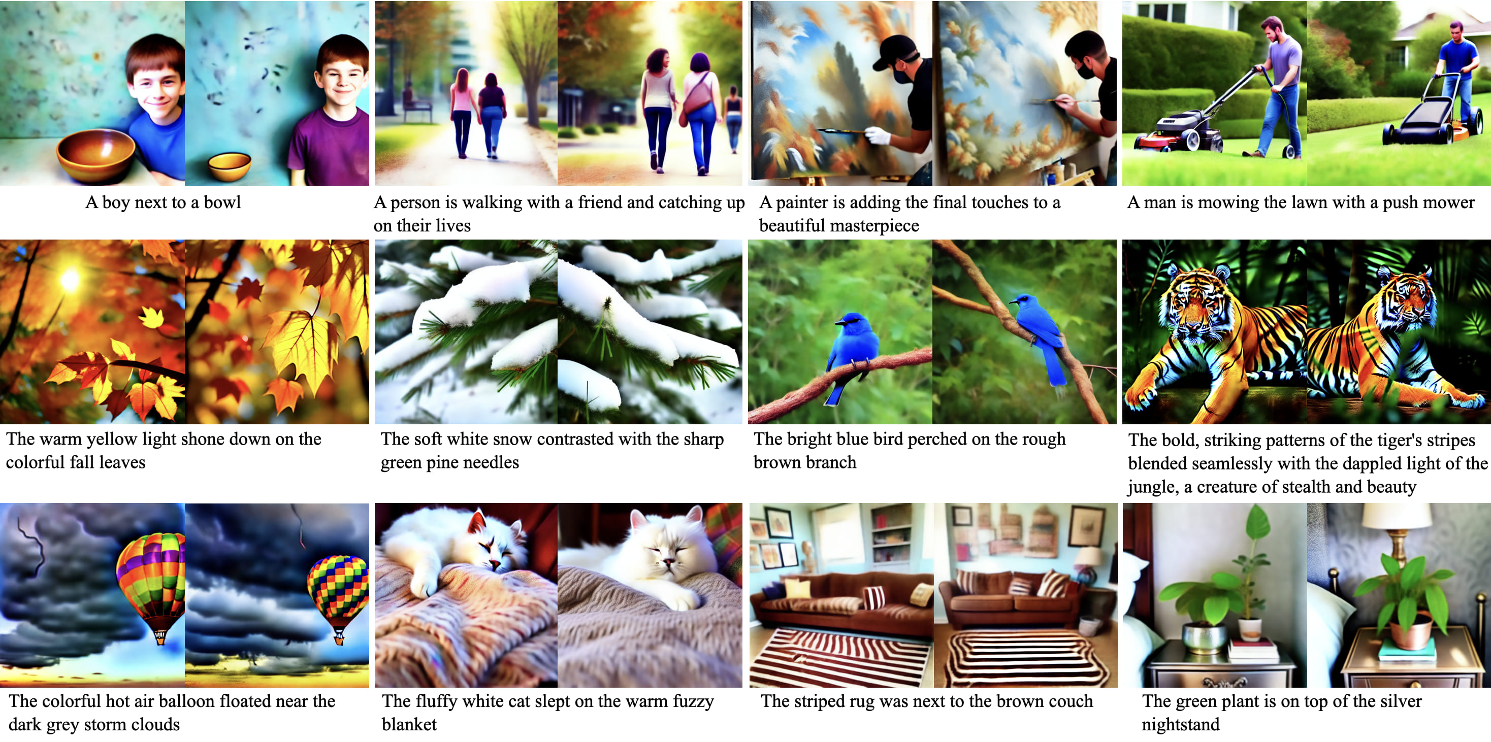
Figure 29: Images with prompt from Spatial, Non-spatial, and Complex sub-dataset

We compare our method with Stable Difussion v1-5, StructureDiffusion (Feng et al., 2022) and Attend-and-Excite (Phung et al., 2023). The qualitative results are present in Figure 24. Clearly, baseline methods all tend to neglect objects in the prompt. Additionally, we provide more examples of images generated by our method in Appendix A.4, including prompts from Object Relationship and Complex sub-datasets from T2I-CompBench. As can be seen, our method is also able to generate faithful images for prompts that describe actions, like “A person is walking with a friend and catching up on their lives”, and complex prompts that include multiple attributes for each object, like “The bold, striking patterns of the tiger’s stripes blended seamlessly with the dappled light of the jungle, a creature of stealth and beauty” (see Figure 29).

4.3 Ablation Studies

Our method comprises two pivotal components: a pre-trained BLIP-2 model and SDS with SD. Among these, BLIP-2 assumes a more critical role in the image generation process, ensuring that the generated images faithfully adhere to the provided texture instructions. To harmoniously integrate these two components, extensive exploratory experiments were conducted to identify the optimal combination. In our ablation studies, we randomly sample 60 images, with 20 images selected from each of the three Attribute-binding datasets (color/shape/texture) within T2I-CompBench for each experiment.

SDS Weight

We adaptively scale the BLIP-2 gradient so that its norm is twice that of the SDS gradient and conduct the exploration to determine the most suitable weights for SDS. We observe that higher values of the CFG factor and SDS weight $w_{2}$ can produce clearer and more realistic images but at the cost of reduced image-text alignment. Conversely, extremely low SDS weights, such as those starting below 800, struggle to generate clear and natural-looking images. Similarly, when CFG values are low, for instance, at 10, the image quality and alignment are both harmed. The most suitable SDS weight falls within the range of 800 to 1000, ideally paired with CFG values of 20 or 30. The quantitative result is presented in Appendix C.1. We further explored the scaled SDS weight and found a sweet point at starting with 800 and gradually decreasing to 400, with CFG equal to 30 (see Table 5).

BLIP-2 Weight

Since we optimize the image with the gradient of BLIP-2 and SDS separately, we also investigate the frequency and weight of BLIP-2 $w_{1}$ at each iteration. The results are shown in Table 6. The BLIP gradient norm should always be larger than SDS to ensure a better alignment with the text, yet an overemphasis on it can lead to the generation of noisy and unrealistic images, which ultimately reduces the alignment score.

Table 5: Results of scaling SDS weight $w_{2}$ with CFG scale of 20 & 30

cfg \$w_{2}$	800 $\to$ 400	1000 $\to$ 500	1500 $\to$ 500
20	63.77 (71.32/44.78/75.21)	64.12 (74.36/48.49/70.53)	60.67 (71.23/42.89/68.12)
30	69.43 (79.98/49.08/79.23)	67.43 (75.76/48.36/78.17)	63.34 (74.00/43.19/72.89)

Table 6: The influence of BLIP-2 weight $w_{1}$ and frequency.

f \ $w_{1}$	1	2	3
1	59.97 (75.08/39.44/65.37)	67.43 (75.76/48.36/78.17)	62.36 (65.12/46.91/75.04)
2	61.55 (72.96/46.66/65.02)	64.29 (75.52/43.77/73.59)	-

EMA-restart

We explore the effectiveness of the EMA-restart strategy with different start iteration locations $e_{s}$ and restart intervals $e_{rs}$, and the results are presented in Table 4. In general, we find that combinations of start $\&$ restart that resulted in 2$\sim$3 times EMA replacements can significantly benefit the result.

Random Noise Our experiments indicate that introducing random noise to $\mathbf{z}$ after each optimization iteration enhances result robustness. The results of different random noise scales are displayed in Appendix C.1 Table 9.

5 Related Work

Controllable Image Generation.

To facilitate flexible image generation capable of meeting diverse requirements, achieving controllable image generation has become a prominent focus in recent times. A prevalent approach is guidance generation. This kind of method obviates the necessity of training a diffusion model from scratch with specific conditions and instead offers direction by pre-existing specialized models or loss functions for the reverse process of the diffusion model. An early attempt in this direction was GLIDE (Nichol et al., 2021) and classifier-free guidance (Ho & Salimans, 2022), which facilitate a diffusion model in generating images that align with textual descriptions. To satisfy arbitrary requirements like textual descriptions, layouts, or segmentation, Universal Guidance (Bansal et al., 2023) is proposed. It leverages pre-existing models to offer iterative directions during the reverse process of a diffusion model. Specifically, to achieve control over multi-faced objects within the prompts, current methods typically involve the incorporation of prior layout information, either by utilizing the bound boxes as guidance (Lian et al., 2023) or injecting grounding information into new trainable layers (Li et al., 2023b; Chen et al., 2023b). Furthermore, it has been observed that cross-attention primarily governs the handling of object-related information. Consequently, various approaches have been developed that involve modifying cross-attention mechanisms to ensure that the diffusion model sufficiently attends to all objects specified in the prompts (Feng et al., 2022; Kim et al., 2023b; Chefer et al., 2023). Notably, approaches that combine bounding boxes with attention control have demonstrated improved performance in this regard (Phung et al., 2023; Wang et al., 2023b).

What sets our method apart is the central role played by a discriminative Vision-Language Model (VLM) during the image synthesis process, rather than relying on the generative model. Additionally, our approach is entirely training-free and does not necessitate the inclusion of extra information, such as layout details or object indices.

Image Generation via Model Inversion

Model inversion refers to the invert process of general model training, i.e., optimizing the input, which is initially randomly initialized, while keeping the well-trained model parameters unchanged (Mahendran & Vedaldi, 2015). An early endeavor in this direction was DeepDream (Alexander Mordvintsev & Tyka, 2015), which sought to create images corresponding to specific classes given a classification model, by producing high responses for specific classes in the output layer of the model. However, the reverse classification process posed significant challenges. During the optimization process of model inversion, it’s easy to get stuck in local optima and end up with very unrealistic images that can be regarded as adversarial examples (Goodfellow et al., 2014; Wang & Torr, 2022). Subsequent methods, such as DeepInversion (Yin et al., 2020) and CaG (Wang & Torr, 2022), introduced various regularization techniques to improve the identifiability of generated images. However, the generated images were still far from natural and lacked coherency. Notably, VQGAN-CLIP (Crowson et al., 2022) emerged as a successful example within this category of methods. It generates images by inversely applying a trained VQGAN model (Esser et al., 2021) using a loss function that measures the similarity of image and text embeddings from a CLIP model (Radford et al., 2021) and incorporates augmentation regularization. Nevertheless, VQGAN-CLIP did not delve into the impact of various augmentation methods and the mechanism underlying the effectiveness of augmentation regularization, even in subsequent studies.

We are the first to comprehensively investigate the underlying mechanism of augmentation regularization, and how to choose the appropriate augmentation techniques.

6 Conclusion and Discussion

In this study, we introduce a novel framework for image generation that enhances controllability. Our approach is rooted in a fresh perspective on comprehending the recent advancements in text-to-image synthesis models like DALLE3 as a learned inversion function of the VLM. Subsequently, we propose a direct inversion of the VLM through optimization, harnessing the full potential of text and image alignment inherent in VLMs. We elucidate the effectiveness of augmentation regularization that facilitates generating faithful images via VLM inversion. Furthermore, we enhance our method by incorporating SDS and thoroughly explore the effective synergy between it and VLM, achieving correctly generating fidelity images.

Nonetheless, our method does have limitations. For instance, the stability of the generation process is not as good as SOTA DPMs, due to the optimization nature. Occasionally mismatches or unrealistic images still occur. In this work, we only demonstrated working with the BLIP-2 model as a referee, which we found to struggle with spatial information. Instructions involving spatial relationships such as “to the left/right”, “on the top/bottom”, etc., can be challenging to follow. Our work can be further strengthened if we can incorporate multiple referees with diverse knowledge, e.g., grounding VQA model, detection models, segmentation models, etc. Such a model zoo setting has been demonstrated effective in domain generalization (Shu et al., 2021; Dong et al., 2022; Chen et al., 2023c). As the referees get more sophisticated, memory-efficient optimization (Anil et al., 2019; Baydin et al., 2022; Malladi et al., 2024) can be utilized to reduce the computation load and promote scalability.

Despite these limitations, we are introducing a novel direction and highlighting its significant potential. For all modalities, evaluating the generated samples is a challenging task. For example, we have FID (Heusel et al., 2017) for images, but such a well-accepted criterion is missing for 3D generation. Nevertheless, as long as there exist powerful discriminative models that can tell whether the generated samples are good or not, they can be utilized in a training-free fashion by extending our method to achieve a significant boost in conditional generation across every modality. Our goal is to inspire further investigations along this path, revealing the unexplored capabilities of discriminative models in generative tasks. Currently, we have only explored basic models in image generation, and we hope to inspire more future works to leverage more powerful discriminative and language models, thereby developing more robust capabilities.

Appendix A Appendix

A.1 Importance of discriminative component in conditional generation

We present both quantitative and qualitative results, showing that the discriminative module plays a more central role in aligning with the condition for current text-to-image DPMs. Table 7 shows the result of the BLIP-VQA score on the Attribute-binding sub-dataset of T2I-CompBench of Stable Diffusion v1.5 with different classifier-free-guidance (CFG) scales; clearly, a better alignment of text and image can be achieved by a larger CFG scale. We further present the images generated by the traditional generation process of Stable Diffusion v1.5 with CFG coefficient 7.5, 30, and the Score Distillation Sampling (SDS) process separately. The results indicate that when strong conditions come along, a smaller CFG also performs poorly, and the higher CFG results in comparative image quality but higher consistency with text.

Table 7: The BLIP-VQA score of Stable Diffusion v1.5 with CFG 7.5 and 30 on Attribute-binding dataset

	color	shape	texture
cfg=7.5	0.3632	0.3490	0.3985
cfg=30	0.4012	0.4018	0.4386

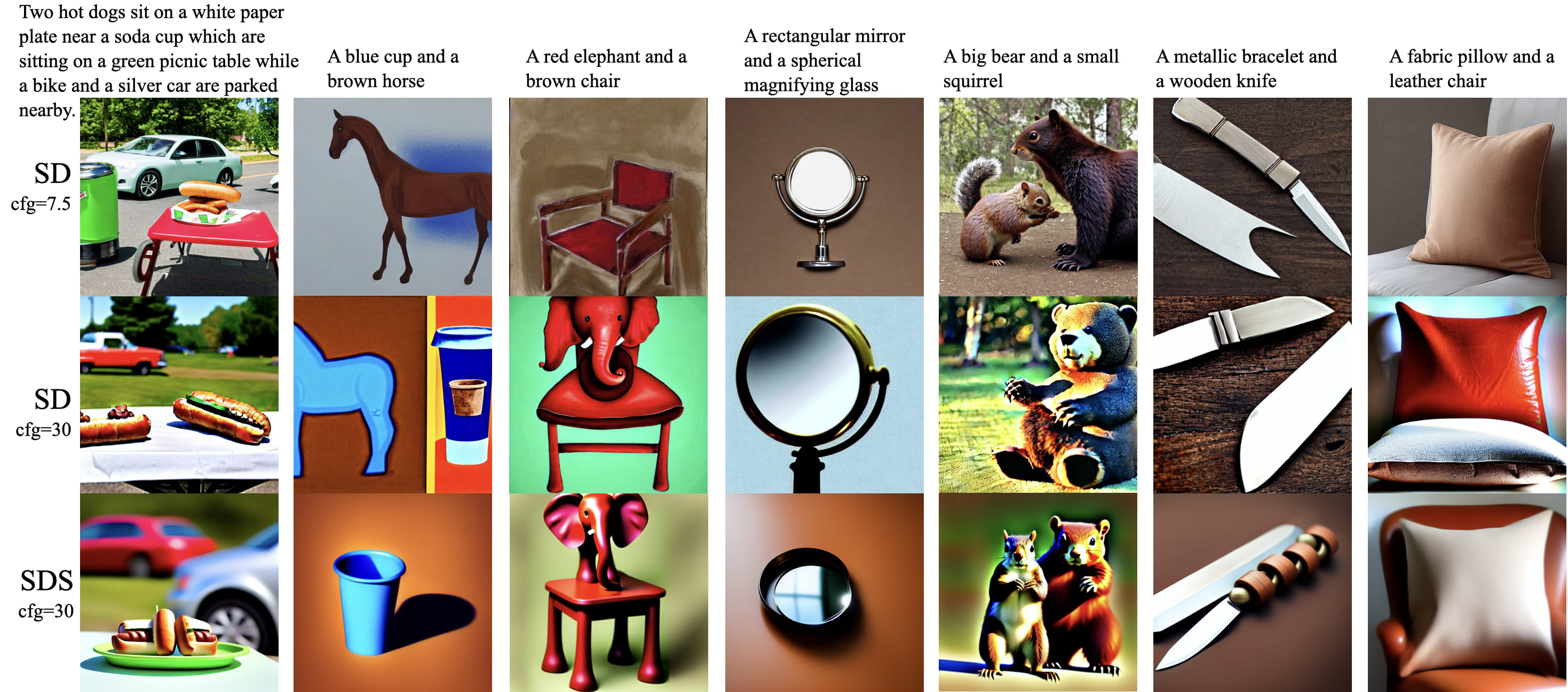
Figure 25: A comparison of the images generated from the Stable Diffusion (SD) reverse process with CFG scale=7.5, 30 and the Score Distillation Sampling (SDS) process with CFG scale=30.

A.2 Detailed BLIP-2 losses

We directly utilize the training losses of the BLIP-2 model (Li et al., 2021, 2022, 2023a), except the image-text contrastive (ITC) loss, because it requires a large batch size that is not suitable for text-to-image generation tasks. The image-text matching loss ($\mathcal{L}_{itm})$ focuses on learning how images and texts align closely. It’s a simple binary cross-entropy loss: the model predicts if an image and text pair match or not, using a linear layer called the ITM head based on their combined features. The caption-generation loss ($\mathcal{L}_{cg}$) aims to generate textual descriptions given an image. It optimizes a cross-entropy loss which trains the BERT module to maximize the likelihood of the text in an autoregressive manner. A label smoothing of 0.1 is adopted when computing the loss.

Specifically,

$$\mathcal{L}_{itm}=\mathbb{E}_{(I,T)}H(\mathbf{y}^{itm},\mathbf{p}^{itm}(I,T))),$$ (2)

where $H$ denotes the cross-entropy function, $\mathbf{y}^{itm}$ is a 2-dimensional one-hot vector representing the ground-truth label of whether $I$ and $T$ is a match, $\mathbf{p}^{itm}$ is the output of the ITM head.

$$\mathcal{L}_{cg}=\mathbb{E}_{(I,\widehat{T})}H(\mathbf{y}^{mask},\mathbf{p}^{mask}(I,\widehat{T})),$$ (3)

where $\widehat{T}$ denotes the text with mask, and $\mathbf{p}^{mask}(I,\widehat{T})$ denotes the BERT module’s output for a masked token, and $\mathbf{y}^{mask}$ is a one-hot vocabulary distribution in which the value of the ground-truth token is set to 1.

A.3 Exploration on augmentation methods for VLM inversion

Here we show the impact of adding random resized crop and random horizontal flip augments, and straightforwardly illustrate the potential reasons through BLIP-2 loss that measures the semantic consistency.

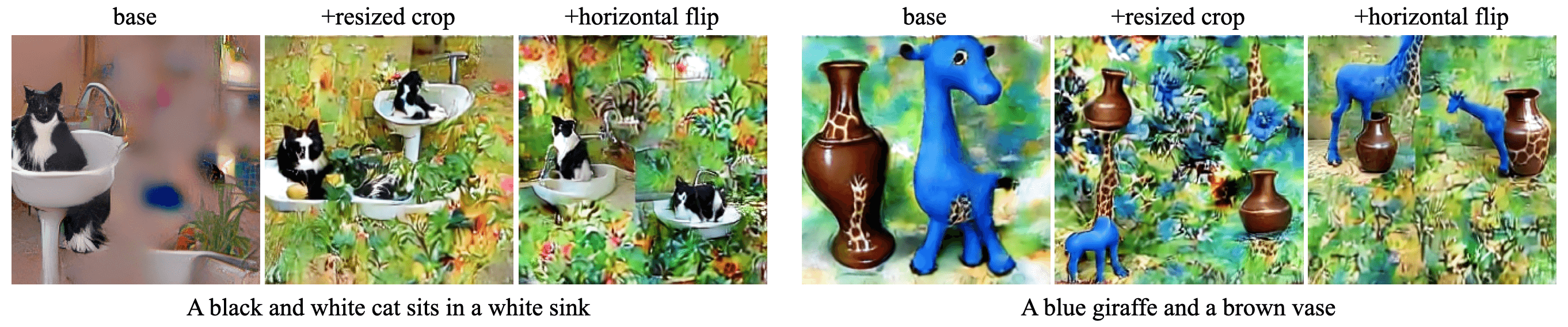
Figure 26: Images with our base augmentation methods (random affine, random perspective, color-jitter, random erasing, and Gaussian noise), base + random resized crop, and base + random horizontal flip.

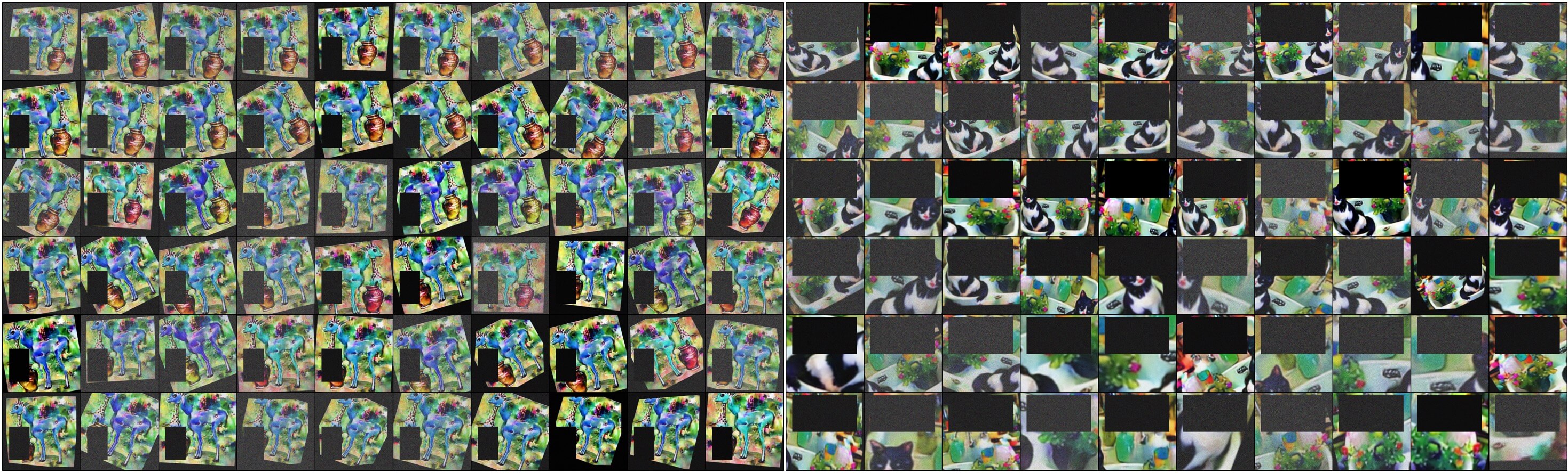
Figure 27: Sorted augmented images sorted in ascending order of BLIP-2 loss $L(\mathbf{x},\mathbf{y})$. In the left image, the horizontally flipped images exhibit higher loss. Since all of our captions contain multiple objects, incorporating horizontal flip together with random erasing easily leads to semantic inconsistencies within the same equivalence class. The right image shows that images augmented through resized cropping have a larger loss, which clearly shows altered semantic information.

A.4 More images of our method

We show more images generated by our method with the prompts sampled from the attribute-biding, spatial $\&$ non-spatial, and complex sub-datasets of T2I-CompBench, indicating our method’s effectiveness in generating images with different types of prompts.

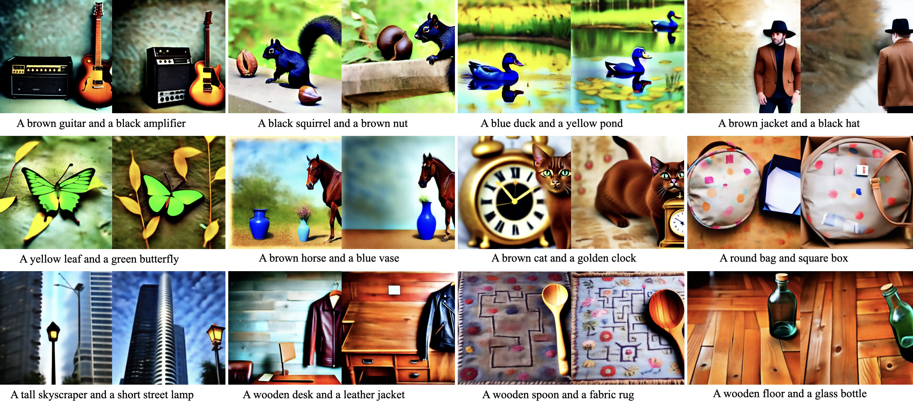
Figure 28: Images with prompt from Attribute-binding sub-dataset

A.5 Role of BLIP-2 inversion and SDS during Optimization

Evolution of individual BLIP-2 inversion, SDS, and our method (BLIP-2+SDS)

To better illustrate the effect of the two components of our method, we present the image evolution during the optimization of the two components work separately and together (Figure 30 and 31). Apparently, BLIP-2 inversion can strictly follow the prompt, while SDS tends to partially follow the prompt and neglect some objects contained in the prompt. Besides, for SDS optimization, images can change a lot during evolution, especially when encountering multiple objects in the prompt (see Figure 30), showing that introducing the instruction by cross attention is kind of fragile, the information contained in the prompt is always incompletely captured and unstable. Things are totally different in BLIP-2 inversion; the instruction is well followed, while the perceptual image quality is kind of weak. When these two components work together, better performance is achieved.

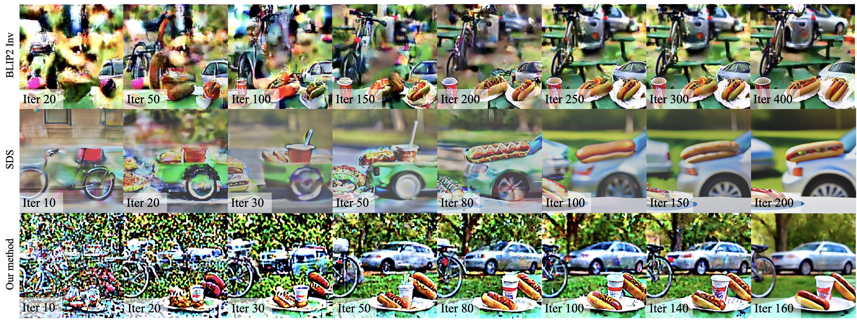
Figure 30: Image evolution of prompt “Two hot dogs sit on a white paper plate near a soda cup which are sitting on a green picnic table while a bike and a silver car are parked nearby”.

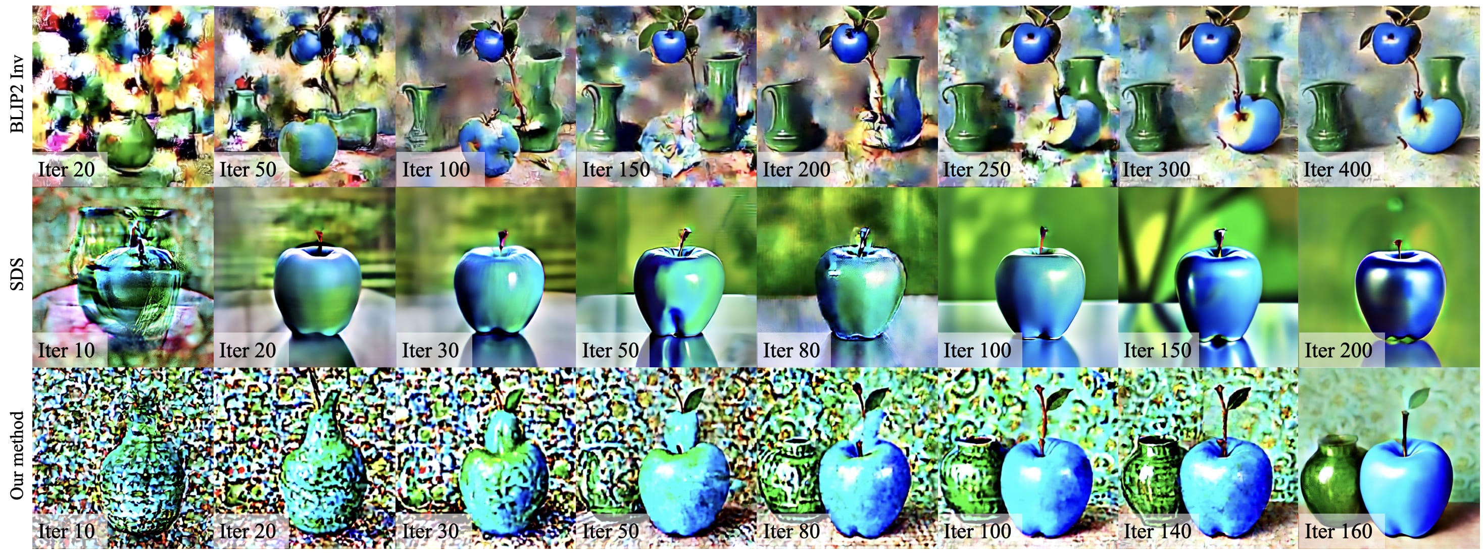
Figure 31: Images evolution of prompt “A blue apple and a green vase”.

Visualization of the gradient of BLIP-2 and SDS

To gain a more intuitive understanding of the distinct roles of the two components in our method, we visualized the gradients provided by each module (see Figure 33). Our approach to visualization is quite straightforward. We directly selected the first three (out of four) channels and then presented them in the form of images. It is evident that the gradient information from BLIP-2 is primarily concentrated on the objects, especially those with incorrectly generated attributes or those that are omitted. On the other hand, the gradients provided by SDS are more comprehensive, clearly outlining the contours of objects while also optimizing the background. Although our visualization method is direct and somewhat rudimentary, it effectively highlights the distinct functions of each module. For example, with the prompt “a blue apple and a green vase”, the SDS gradient reveals the outlines of two apples, while the BLIP-2 gradient focuses on one of the apples with the wrong attribute, attempting to transform it into a vase that matches the text description (see Figure 33).

Figure 33: Visualization of the Gradient of BLIP-2 and SDS. The images, the gradient of BLIP-2, and the gradient of SDS visualization are separately shown from top to bottom row.

A.6 Limitations of our method

Although our method is simple and effective, it still has certain shortcomings (see Figure 34). First, our method struggles to generate images with accurate positional information. We attribute this to BLIP-2’s insensitivity to capturing location details. Individual BLIP-2 inversion, despite achieving highly accurate attribute matching, performs poorly in the Spatial subset (see BLIP-2 Inv result in Table 3). Additionally, our method often generates images that directly incorporate the prompt. This may be due to the direct involvement of a BERT text encoder in the pre-trained BLIP-2 contained in our current approach. These issues are also encountered in DALLE3. Lastly, as our method does not directly utilize a specialized image generation model, it sometimes produces images that are not entirely realistic. For instance, to achieve correct attribute matching, our method may generate images where multiple objects are merged into one, which seems quite unrealistic.

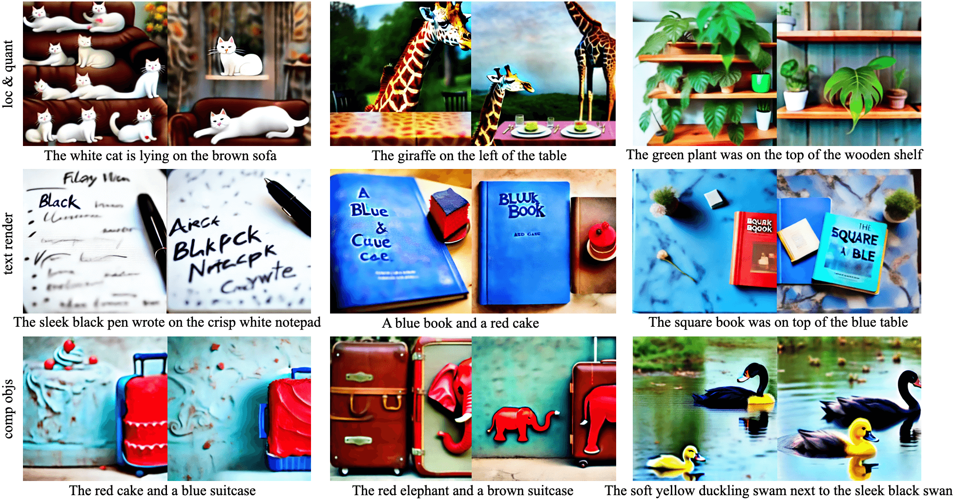
Figure 34: Limitations of our method.

Appendix B Technical Details

We introduce two propositions, both of which state that the smoothed version of $f$ by taking the expectation of the noise $\mathbb{E}_{\epsilon\sim P}f(x+\epsilon)$ has nicer property. Proposition B.1 states that the smoothed function has a higher smoothness (roughly speaking, it can take a higher degree of derivatives), and Proposition B.2 states that the smoothed function has a smaller condition number, which may lead to faster convergence rate when applying gradient descent for minimization.

Before introducing these two propositions, we state some necessary terminologies. We say a function $f$ has smoothness $m$ if $f$ is in the Sobolev space $H^{m}(\mathbb{R}^{d})$. The Fourier transform of $f\in L_{1}(\mathbb{R}^{d})$ is given by

$$\mathcal{F}(f)(\omega)=(2\pi)^{-d/2}\int_{\mathbb{R}^{d}}f(x)e^{-ix^{T}\omega}dx.$$

The characteristic function of a random variable $\epsilon$ following distribution $P$ is defined by $\varphi(t)=\mathbb{E}_{\epsilon\sim P}e^{i\epsilon^{\top}t}$. Let $\partial^{2}f(x)$ be the Hessian matrix on $x\in\mathbb{R}^{d}$. For two positive matrices $A,B$, we write $A\preceq B$ (or $B\succeq A$) if $B-A$ is semi-positive definite.

Proposition B.1 (Improved smoothness).

Let $f\in H^{m}(\mathbb{R}^{d})$. Assume that the characteristic function of the noise $\epsilon$ with mean zero satisfies

$$\varphi(t)\leq c_{1}(1+\|\omega\|^{2})^{-m_{1}/2},\forall\omega\in\mathbb{R}^{d}.$$

Then $g(x)\coloneqq\mathbb{E}_{\epsilon}f(x+\epsilon)$ has smoothness at least $m+m_{1}$, i.e., $g\in H^{m+m_{1}}(\mathbb{R}^{d})$. Furthermore, if $\epsilon$ is Gaussian, then $\mathbb{E}_{\epsilon}f(x+\epsilon)$ has infinite smoothness, i.e., for any $m_{2}>0$, $g\in H^{m+m_{2}}(\mathbb{R}^{d})$. Moreover, $\widetilde{L}_{y}$ is $\sqrt{\frac{2R^{2}}{\pi\sigma^{2}}}$-Lipschitz when $\epsilon\sim\mathcal{N}(0,\sigma^{2}I)$ and $L_{y}:\mathbb{R}^{d}\mapsto\mathbb{R}$ with $R\geq\sup_{x\in\mathbb{R}^{d}}|L_{y}(x)|$.

Proof.

Since $f\in H^{m}(\mathbb{R}^{d})$, it can be shown that (Adams & Fournier, 2003)

$$\int_{\mathbb{R}^{d}}|\mathcal{F}(f)(\omega)|^{2}(1+\|\omega\|_{2}^{2})^{m}{\rm d}\omega<\infty.$$

The Fourier inversion theorem implies that

$$g(x)=\mathbb{E}_{\epsilon}f(x+\epsilon)= \mathbb{E}_{\epsilon}\int_{\mathbb{R}^{d}}\mathcal{F}(f)(\omega)e^{i(x+\epsilon)^{\top}\omega}{\rm d}\omega$$

$$= \mathbb{E}_{\epsilon}\int_{\mathbb{R}^{d}}\mathcal{F}(f)(\omega)e^{ix^{\top}\omega}e^{i\epsilon^{\top}\omega}{\rm d}\omega$$

$$= \int_{\mathbb{R}^{d}}\mathcal{F}(f)(\omega)e^{ix^{\top}\omega}\varphi(\omega){\rm d}\omega.$$

Therefore, we have

$$\int_{\mathbb{R}^{d}}|\mathcal{F}(g)(\omega)|^{2}(1+\|\omega\|_{2}^{2})^{m+m_{1}}{\rm d}\omega$$

$$= \int_{\mathbb{R}^{d}}|\mathcal{F}(f)(\omega)|^{2}|\varphi(\omega)|^{2}(1+\|\omega\|_{2}^{2})^{m+m_{1}}{\rm d}\omega$$

$$\leq c_{1}^{2}\int_{\mathbb{R}^{d}}|\mathcal{F}(f)(\omega)|^{2}(1+\|\omega\|_{2}^{2})^{m}{\rm d}\omega<\infty,$$

which implies $g\in H^{m+m_{1}}(\mathbb{R}^{d})$.

Similarly, if $\epsilon$ is Gaussian, we have $\varphi(\omega)=e^{-\frac{1}{2}\sigma^{2}\omega^{2}}$. Hence, for any $m_{2}>d/2$, it holds that

$$\int_{\mathbb{R}^{d}}|\mathcal{F}(g)(\omega)|^{2}(1+\|\omega\|_{2}^{2})^{m+m_{2}}{\rm d}\omega$$

$$= \int_{\mathbb{R}^{d}}|\mathcal{F}(f)(\omega)|^{2}e^{-\sigma^{2}\omega^{2}}(1+\|\omega\|_{2}^{2})^{m+m_{1}}{\rm d}\omega$$

$$\leq C\int_{\mathbb{R}^{d}}|\mathcal{F}(f)(\omega)|^{2}(1+\|\omega\|_{2}^{2})^{m}{\rm d}\omega<\infty,$$

for some constant $C>0$, which implies $g\in H^{m+m_{2}}(\mathbb{R}^{d})$.

The proof of Lipschitz continuity follows from known proofs. Here, we adopt and expand the proof of Lemma 1 of (Salman et al., 2019), which shows that $\widetilde{L}_{y}$ is $\sqrt{\frac{2}{\pi}}$-Lipschitz when $\epsilon\sim\mathcal{N}(0,I)$ and $L_{y}:\mathbb{R}^{d}\mapsto\mathbb{R}$ with $L_{y}(x)\in[0,1]$. By the mean value theorem, there exists some $c$ interpolating $x$ and $x^{\prime}$ such that

$$\|\widetilde{L}_{y}(x)-\widetilde{L}_{y}(x^{\prime})\|=\|\nabla\widetilde{L}_{y}(c)^{\top}(x^{\prime}-x)\|=\|\nabla\widetilde{L}_{y}(c)^{\top}\frac{(x^{\prime}-x)}{\|(x^{\prime}-x)\|}\|(x^{\prime}-x)\|\|\leq|\widetilde{L}_{y}(c)^{\top}v|\|(x^{\prime}-x)\|.$$

where $v=\frac{(x^{\prime}-x)}{\|(x^{\prime}-x)\|}$ is a unit vector. Thus, the desired statement holds if $|\nabla\widetilde{L}_{y}(c)^{\top}v|\leq\sqrt{\frac{2R^{2}}{\pi\sigma^{2}}}$ for any unit vector $v$. With $\epsilon=t-x$ (and the symmetry of the Gaussian), we have $\widetilde{L}_{y}(x)=\frac{1}{\sigma^{d}(2\pi)^{d/2}}\int_{\mathbb{R}^{d}}L_{y}(t)\exp\left(-\frac{1}{2\sigma^{2}}\|x-t\|^{2}\right)dt$ and hence

$$\nabla\widetilde{L}_{y}(x)=\frac{1}{\sigma^{d}(2\pi)^{d/2}}\int_{\mathbb{R}^{d}}L_{y}(t)\frac{1}{\sigma^{2}}(t-x)\exp\left(-\frac{1}{2\sigma^{2}}\|x-t\|^{2}\right)dt.$$

Thus, by using $R\geq\sup_{x\in\mathbb{R}^{d}}|L_{y}(x)|$ and classical integration of the Gaussian density (e.g., see Salman et al., 2019),

$$|\nabla\widetilde{L}_{y}(x)^{\top}v| \leq\frac{R}{\sigma^{2}\sigma^{d}(2\pi)^{d/2}}\int_{\mathbb{R}^{d}}|(x-t)^{\top}v|\exp\left(-\frac{1}{2\sigma^{2}}\|x-t\|^{2}\right)dt$$

$$=\frac{R}{\sigma^{2}\sigma\sqrt{2\pi}}\int_{-\infty}^{\infty}|s|\exp\left(-\frac{s^{2}}{2\sigma^{2}}\right)ds$$

$$=\sqrt{\frac{2R^{2}}{\pi\sigma^{2}}}.$$

where the last line follows from the fact that $\int_{-\infty}^{\infty}|s|\exp\left(-\frac{s^{2}}{2\sigma^{2}}\right)ds=2\sigma^{2}$. ∎

A smaller Lipschitz constant can benefit optimization because the convergence speed tends to decrease as the Lipschitz constant increases, where typically the learning rate also needs to be smaller to achieve the convergence rate as the Lipschitz constant increases (Ghadimi & Lan, 2013; Bertsekas, 2016). For example, the convergence rate degrades (more than quadratically) as the Lipschitz constant increases (linearly) in Theorem 3 of (Lei et al., 2019) for SGD on nonconvex optimization (since their constant $C$ depends on the Lipschitz constant in its proof). Therefore, the smoothness gained by the random augmentation can benefit optimization.

Proposition B.2 (Improved condition number of convex optimization).

Let $f(x)$ be a convex function with continuous $\partial^{2}f(x)$ and

$$\mu I\preceq\partial^{2}f(x)\preceq LI,\forall x\in\mathbb{R}^{d},$$

where $I$ is an identity matrix and $\mu,L$ are two positive constants. Assume $\epsilon\sim P$ has mean zero and support $\mathbb{R}^{d}$, and $\partial^{2}\mathbb{E}_{\epsilon}f(x+\epsilon)=\mathbb{E}_{\epsilon}\partial^{2}f(x+\epsilon)$. Then

$$\mu_{1}I\preceq\partial^{2}g(x)\preceq L_{1}I,\forall x\in\mathbb{R}^{d},$$

with $\mu_{1}\geq\mu$ and $L_{1}\leq L$, where $g(x)=\mathbb{E}_{\epsilon}f(x+\epsilon)$. In addition, the inequalities are strict, i.e., $\mu_{1}>\mu$ and $L_{1}<L$, if there exist $x_{0},x_{1}\in\mathbb{R}^{d}$ and constants $c_{1},c_{2}>0$ such that

$$\partial^{2}f(x_{0})\succeq(\mu+c_{1})I,\partial^{2}f(x_{1})\preceq(L-c_{2})I.$$ (4)

Remark B.3.

Theorem 2.2.14 of Nesterov et al. (2018) states that an upper bound of the gradient descent is

$$\|x_{k}-x^{*}\|\leq\left(1-\frac{2}{1+\kappa}\right)^{k}\|x_{0}-x^{*}\|,$$

where $\kappa=L/\mu$ is the condition number. A larger $\kappa$ indicates a slower convergence rate. Proposition B.2 states that for the smoothed version of $f$, it can have a smaller condition number, thus indicating a faster convergence rate for gradient descent.

Proof.

Direct computation shows that

$$\partial^{2}g(x)=\mathbb{E}_{\epsilon}\partial^{2}f(x+\epsilon)=\int_{\mathbb{R}^{d}}\partial^{2}f(x+\epsilon){\rm d}P,$$

which clearly satisfies

$$\mu_{1}I\preceq\partial^{2}g(x)\preceq L_{1}I,\forall x\in\mathbb{R}^{d},$$

with $\mu_{1}\geq\mu$ and $L_{1}\leq L$, since $\int_{\mathbb{R}^{d}}{\rm d}P=1$.

Suppose (4) holds. We only show $\mu_{1}>\mu$, since $L_{1}<L$ can be shown similarly. By the continuity of $\partial^{2}f(x)$, there exists a neighbor hood $B(x_{0},\delta)$ with $\delta>0$ such that $\partial^{2}f(x_{0})\succeq(\mu+c_{1}^{\prime})I$ with some positive constant $c_{1}^{\prime}>0$. Hence,

$$\partial^{2}g(x)= \int_{\mathbb{R}^{d}}\partial^{2}f(x+\epsilon){\rm d}P$$

$$= \int_{\mathbb{R}^{d}\backslash B(x_{0},\delta)}\partial^{2}f(x+\epsilon){\rm d}P+\int_{B(x_{0},\delta)}\partial^{2}f(x+\epsilon){\rm d}P$$

$$\succeq \mu I\int_{\mathbb{R}^{d}\backslash B(x_{0},\delta)}{\rm d}P+(\mu+c_{1}^{\prime})I\int_{B(x_{0},\delta)}{\rm d}P,$$

which implies $\mu_{1}>\mu$, since $\int_{\mathbb{R}^{d}}{\rm d}P=1$ and $\int_{B(x_{0},\delta)}{\rm d}P>0$. Similarly, $L_{1}<L$. This finishes the proof. ∎

Appendix C Experiment Details

We optimize the randomly initialized $\mathbf{z}$ for 160 iterations. In the first 150 iterations, $\mathbf{z}$ is firstly updated using gradients provided by $\mathcal{L}_{align}$ backpropagation via an Adam optimizer. Subsequently, it is further refined using gradients provided by SDS through an SGD optimizer without momentum. The norm of the gradient from BLIP-2 is always twice the gradient from SDS; a noise $\epsilon_{z}\sim\mathcal{N}(0,0.04)$ is added on the updated $\mathbf{z}$. In the last 10 iterations, $\mathbf{z}$ is updated solely based on the gradients from SDS. We initialize the learning rate at 1.0, which then gradually diminishes to 0.5 following a cosine decay schedule. The SDS weight gradually decays from 800 to 400 following a cosine decay rate. We also implement exponential moving average (EMA) restart at 40 and 100 iterations. All experiments are conducted on the Tesla V100 gpus.

C.1 Abation results

The results of ablation explorations on the constant SDS weight and random noise scale are represented in Table 8 and 9.

Table 8: Result of different CFG-scale and SDS weight $w_{2}$

cfg / $w_{2}$	800	1000	1500	2000
10	56.52 (70.28/35.98/63.32)	57.70 (73.87/36.24/64.83)	54.40 (67.60/35.14/63.47)	52.62 (62.58/32.85/62.43)
20	62.74 (74.28/40.78/73.21)	61.08 (71.06/39.59/72.58)	60.39 (67.86/40.05/72.26)	58.06 (68.34/39.19/66.67)
30	62.18 (73.32/41.01/74.12)	60.90 (72.36/40.19/70.50)	59.78 (66.98/42.64/69.72)	56.70 (66.93/39.59/66.59)

Table 9: Results of adding random noise on z

$\sigma$	0.05	0.1	0.2	0.3
vqaScore	68.21 (79.02/46.50/79.07)	70.88 (81.12/51.62/80.00)	71.04 (79.54/51.35/83.23)	64.57 (70.54/43.66/79.50)

References

- Adams & Fournier (2003) Adams, R. A. and Fournier, J. J. Sobolev Spaces, volume 140. Academic Press, 2003.
- Alexander Mordvintsev & Tyka (2015) Alexander Mordvintsev, C. O. and Tyka, M. Inceptionism: Going deeper into neural networks, 2015. URL https://blog.research.google/2015/06/inceptionism-going-deeper-into-neural.html.
- Anil et al. (2019) Anil, R., Gupta, V., Koren, T., and Singer, Y. Memory efficient adaptive optimization. Advances in Neural Information Processing Systems, 32, 2019.
- Arrieta et al. (2020) Arrieta, A. B., Díaz-Rodríguez, N., Del Ser, J., Bennetot, A., Tabik, S., Barbado, A., García, S., Gil-López, S., Molina, D., Benjamins, R., et al. Explainable artificial intelligence (xai): Concepts, taxonomies, opportunities and challenges toward responsible ai. Information fusion, 58:82–115, 2020.
- Bansal et al. (2023) Bansal, A., Chu, H.-M., Schwarzschild, A., Sengupta, S., Goldblum, M., Geiping, J., and Goldstein, T. Universal guidance for diffusion models. In Proceedings of the IEEE/CVF Conference on Computer Vision and Pattern Recognition, pp. 843–852, 2023.
- Baydin et al. (2022) Baydin, A. G., Pearlmutter, B. A., Syme, D., Wood, F., and Torr, P. Gradients without backpropagation. arXiv preprint arXiv:2202.08587, 2022.
- Bertsekas (2016) Bertsekas, D. Nonlinear Programming. Athena scientific optimization and computation series. Athena Scientific, 2016.
- Betker et al. (2023) Betker, J., Goh, G., Jing, L., Brooks, T., Wang, J., Li, L., Ouyang, L., Zhuang, J., Lee, J., Guo, Y., et al. Improving image generation with better captions. Computer Science. https://cdn. openai. com/papers/dall-e-3. pdf, 2023.
- Cai et al. (2021) Cai, Z., Ravichandran, A., Maji, S., Fowlkes, C., Tu, Z., and Soatto, S. Exponential moving average normalization for self-supervised and semi-supervised learning. In Proceedings of the IEEE/CVF Conference on Computer Vision and Pattern Recognition (CVPR), pp. 194–203, June 2021.
- Chefer et al. (2023) Chefer, H., Alaluf, Y., Vinker, Y., Wolf, L., and Cohen-Or, D. Attend-and-excite: Attention-based semantic guidance for text-to-image diffusion models. ACM Transactions on Graphics (TOG), 42(4):1–10, 2023.
- Chen et al. (2023a) Chen, J., Yu, J., Ge, C., Yao, L., Xie, E., Wu, Y., Wang, Z., Kwok, J., Luo, P., Lu, H., et al. Pixart-: Fast training of diffusion transformer for photorealistic text-to-image synthesis. arXiv preprint arXiv:2310.00426, 2023a.
- Chen et al. (2020) Chen, T., Kornblith, S., Norouzi, M., and Hinton, G. A simple framework for contrastive learning of visual representations. In International conference on machine learning, pp. 1597–1607. PMLR, 2020.
- Chen et al. (2023b) Chen, X., Liu, Y., Yang, Y., Yuan, J., You, Q., Liu, L.-P., and Yang, H. Reason out your layout: Evoking the layout master from large language models for text-to-image synthesis. arXiv preprint arXiv:2311.17126, 2023b.
- Chen et al. (2023c) Chen, Y., Hu, T., Zhou, F., Li, Z., and Ma, Z.-M. Explore and exploit the diverse knowledge in model zoo for domain generalization. In International Conference on Machine Learning, pp. 4623–4640. PMLR, 2023c.
- Chuang et al. (2022) Chuang, C.-Y., Hjelm, R. D., Wang, X., Vineet, V., Joshi, N., Torralba, A., Jegelka, S., and Song, Y. Robust contrastive learning against noisy views. In Proceedings of the IEEE/CVF Conference on Computer Vision and Pattern Recognition, pp. 16670–16681, 2022.
- Cohen et al. (2019) Cohen, J., Rosenfeld, E., and Kolter, Z. Certified adversarial robustness via randomized smoothing. In international conference on machine learning, pp. 1310–1320. PMLR, 2019.
- Crowson et al. (2022) Crowson, K., Biderman, S., Kornis, D., Stander, D., Hallahan, E., Castricato, L., and Raff, E. Vqgan-clip: Open domain image generation and editing with natural language guidance. In European Conference on Computer Vision, pp. 88–105. Springer, 2022.
- Dangovski et al. (2021) Dangovski, R., Jing, L., Loh, C., Han, S., Srivastava, A., Cheung, B., Agrawal, P., and Soljačić, M. Equivariant contrastive learning. arXiv preprint arXiv:2111.00899, 2021.
- Ding et al. (2023) Ding, L., Hu, T., Jiang, J., Li, D., Wang, W., and Yao, Y. Random smoothing regularization in kernel gradient descent learning. arXiv preprint arXiv:2305.03531, 2023.
- Dong et al. (2022) Dong, Q., Muhammad, A., Zhou, F., Xie, C., Hu, T., Yang, Y., Bae, S.-H., and Li, Z. Zood: Exploiting model zoo for out-of-distribution generalization. Advances in Neural Information Processing Systems Volume 35, 2022.
- Du et al. (2022) Du, Y., Liu, Z., Li, J., and Zhao, W. X. A survey of vision-language pre-trained models. arXiv preprint arXiv:2202.10936, 2022.
- Esser et al. (2021) Esser, P., Rombach, R., and Ommer, B. Taming transformers for high-resolution image synthesis. In Proceedings of the IEEE/CVF conference on computer vision and pattern recognition, pp. 12873–12883, 2021.
- Feng et al. (2021) Feng, R., Lin, Z., Zhu, J., Zhao, D., Zhou, J., and Zha, Z.-J. Uncertainty principles of encoding gans. In International Conference on Machine Learning, pp. 3240–3251. PMLR, 2021.
- Feng et al. (2022) Feng, W., He, X., Fu, T.-J., Jampani, V., Akula, A., Narayana, P., Basu, S., Wang, X. E., and Wang, W. Y. Training-free structured diffusion guidance for compositional text-to-image synthesis. arXiv preprint arXiv:2212.05032, 2022.
- Ghadimi & Lan (2013) Ghadimi, S. and Lan, G. Stochastic first-and zeroth-order methods for nonconvex stochastic programming. SIAM Journal on Optimization, 23(4):2341–2368, 2013.
- Goodfellow et al. (2014) Goodfellow, I. J., Shlens, J., and Szegedy, C. Explaining and harnessing adversarial examples. arXiv preprint arXiv:1412.6572, 2014.
- HaoChen & Ma (2022) HaoChen, J. Z. and Ma, T. A theoretical study of inductive biases in contrastive learning. arXiv preprint arXiv:2211.14699, 2022.
- He et al. (2020) He, K., Fan, H., Wu, Y., Xie, S., and Girshick, R. Momentum contrast for unsupervised visual representation learning. In Proceedings of the IEEE/CVF conference on computer vision and pattern recognition, pp. 9729–9738, 2020.
- Hertz et al. (2023) Hertz, A., Aberman, K., and Cohen-Or, D. Delta denoising score. In Proceedings of the IEEE/CVF International Conference on Computer Vision, pp. 2328–2337, 2023.
- Hessel et al. (2021) Hessel, J., Holtzman, A., Forbes, M., Bras, R. L., and Choi, Y. Clipscore: A reference-free evaluation metric for image captioning. arXiv preprint arXiv:2104.08718, 2021.
- Heusel et al. (2017) Heusel, M., Ramsauer, H., Unterthiner, T., Nessler, B., and Hochreiter, S. Gans trained by a two time-scale update rule converge to a local nash equilibrium. Advances in neural information processing systems, 30, 2017.
- Ho & Salimans (2022) Ho, J. and Salimans, T. Classifier-free diffusion guidance. arXiv preprint arXiv:2207.12598, 2022.
- Ho et al. (2020) Ho, J., Jain, A., and Abbeel, P. Denoising diffusion probabilistic models. Advances in Neural Information Processing Systems, 33:6840–6851, 2020.
- Hu et al. (2022) Hu, T., Zhili, L., Zhou, F., Wang, W., and Huang, W. Your contrastive learning is secretly doing stochastic neighbor embedding. The Eleventh International Conference on Learning Representations, 2022.
- Hu et al. (2023) Hu, T., Chen, F., Wang, H., Li, J., Wang, W., Sun, J., and Li, Z. Complexity matters: Rethinking the latent space for generative modeling. arXiv preprint arXiv:2307.08283, 2023.
- Huang et al. (2023) Huang, K., Sun, K., Xie, E., Li, Z., and Liu, X. T2i-compbench: A comprehensive benchmark for open-world compositional text-to-image generation. arXiv preprint arXiv:2307.06350, 2023.
- Jia et al. (2021) Jia, C., Yang, Y., Xia, Y., Chen, Y.-T., Parekh, Z., Pham, H., Le, Q., Sung, Y.-H., Li, Z., and Duerig, T. Scaling up visual and vision-language representation learning with noisy text supervision. In International conference on machine learning, pp. 4904–4916. PMLR, 2021.
- Kalantidis et al. (2020) Kalantidis, Y., Sariyildiz, M. B., Pion, N., Weinzaepfel, P., and Larlus, D. Hard negative mixing for contrastive learning. Advances in Neural Information Processing Systems, 33:21798–21809, 2020.
- Kim et al. (2023a) Kim, S., Lee, K., Choi, J. S., Jeong, J., Sohn, K., and Shin, J. Collaborative score distillation for consistent visual synthesis. arXiv preprint arXiv:2307.04787, 2023a.
- Kim et al. (2023b) Kim, Y., Lee, J., Kim, J.-H., Ha, J.-W., and Zhu, J.-Y. Dense text-to-image generation with attention modulation. In Proceedings of the IEEE/CVF International Conference on Computer Vision, pp. 7701–7711, 2023b.
- Kovalev & Gasnikov (2022) Kovalev, D. and Gasnikov, A. The first optimal acceleration of high-order methods in smooth convex optimization. Advances in Neural Information Processing Systems, 35:35339–35351, 2022.
- Lei et al. (2019) Lei, Y., Hu, T., Li, G., and Tang, K. Stochastic gradient descent for nonconvex learning without bounded gradient assumptions. IEEE transactions on neural networks and learning systems, 31(10):4394–4400, 2019.
- Li et al. (2019) Li, B., Chen, C., Wang, W., and Carin, L. Certified adversarial robustness with additive noise. Advances in neural information processing systems, 32, 2019.
- Li et al. (2021) Li, J., Selvaraju, R., Gotmare, A., Joty, S., Xiong, C., and Hoi, S. C. H. Align before fuse: Vision and language representation learning with momentum distillation. Advances in neural information processing systems, 34:9694–9705, 2021.
- Li et al. (2022) Li, J., Li, D., Xiong, C., and Hoi, S. Blip: Bootstrapping language-image pre-training for unified vision-language understanding and generation. In International Conference on Machine Learning, pp. 12888–12900. PMLR, 2022.
- Li et al. (2023a) Li, J., Li, D., Savarese, S., and Hoi, S. Blip-2: Bootstrapping language-image pre-training with frozen image encoders and large language models. arXiv preprint arXiv:2301.12597, 2023a.
- Li et al. (2023b) Li, Y., Liu, H., Wu, Q., Mu, F., Yang, J., Gao, J., Li, C., and Lee, Y. J. Gligen: Open-set grounded text-to-image generation. In Proceedings of the IEEE/CVF Conference on Computer Vision and Pattern Recognition, pp. 22511–22521, 2023b.
- Lian et al. (2023) Lian, L., Li, B., Yala, A., and Darrell, T. Llm-grounded diffusion: Enhancing prompt understanding of text-to-image diffusion models with large language models. arXiv preprint arXiv:2305.13655, 2023.
- Luo et al. (2023) Luo, W., Hu, T., Zhang, S., Sun, J., Li, Z., and Zhang, Z. Diff-instruct: A universal approach for transferring knowledge from pre-trained diffusion models. arXiv preprint arXiv:2305.18455, 2023.
- Ma et al. (2023) Ma, J., Hu, T., Wang, W., and Sun, J. Elucidating the design space of classifier-guided diffusion generation. arXiv preprint arXiv:2310.11311, 2023.
- Mahendran & Vedaldi (2015) Mahendran, A. and Vedaldi, A. Understanding deep image representations by inverting them. In Proceedings of the IEEE conference on computer vision and pattern recognition, pp. 5188–5196, 2015.
- Malladi et al. (2024) Malladi, S., Gao, T., Nichani, E., Damian, A., Lee, J. D., Chen, D., and Arora, S. Fine-tuning language models with just forward passes. Advances in Neural Information Processing Systems, 36, 2024.
- Nesterov et al. (2018) Nesterov, Y. et al. Lectures on convex optimization, volume 137. Springer, 2018.
- Nichol et al. (2021) Nichol, A., Dhariwal, P., Ramesh, A., Shyam, P., Mishkin, P., McGrew, B., Sutskever, I., and Chen, M. Glide: Towards photorealistic image generation and editing with text-guided diffusion models. arXiv preprint arXiv:2112.10741, 2021.
- OpenAI (2023) OpenAI. Dalle-2, 2023. URL https://openai.com/dall-e-2.
- Patrick et al. (2021) Patrick, M., Asano, Y. M., Kuznetsova, P., Fong, R., Henriques, J. F., Zweig, G., and Vedaldi, A. On compositions of transformations in contrastive self-supervised learning. In Proceedings of the IEEE/CVF International Conference on Computer Vision, pp. 9577–9587, 2021.
- Phung et al. (2023) Phung, Q., Ge, S., and Huang, J.-B. Grounded text-to-image synthesis with attention refocusing. arXiv preprint arXiv:2306.05427, 2023.
- Podell et al. (2023) Podell, D., English, Z., Lacey, K., Blattmann, A., Dockhorn, T., Müller, J., Penna, J., and Rombach, R. Sdxl: Improving latent diffusion models for high-resolution image synthesis. arXiv preprint arXiv:2307.01952, 2023.
- Poole et al. (2022) Poole, B., Jain, A., Barron, J. T., and Mildenhall, B. Dreamfusion: Text-to-3d using 2d diffusion. arXiv preprint arXiv:2209.14988, 2022.
- Radford et al. (2021) Radford, A., Kim, J. W., Hallacy, C., Ramesh, A., Goh, G., Agarwal, S., Sastry, G., Askell, A., Mishkin, P., Clark, J., et al. Learning transferable visual models from natural language supervision. In International conference on machine learning, pp. 8748–8763. PMLR, 2021.
- Rombach et al. (2022) Rombach, R., Blattmann, A., Lorenz, D., Esser, P., and Ommer, B. High-resolution image synthesis with latent diffusion models. In Proceedings of the IEEE/CVF Conference on Computer Vision and Pattern Recognition, pp. 10684–10695, 2022.
- Salman et al. (2019) Salman, H., Li, J., Razenshteyn, I., Zhang, P., Zhang, H., Bubeck, S., and Yang, G. Provably robust deep learning via adversarially trained smoothed classifiers. Advances in Neural Information Processing Systems, 32, 2019.
- Shu et al. (2021) Shu, Y., Kou, Z., Cao, Z., Wang, J., and Long, M. Zoo-tuning: Adaptive transfer from a zoo of models. In International Conference on Machine Learning, pp. 9626–9637. PMLR, 2021.
- Sohl-Dickstein et al. (2015) Sohl-Dickstein, J., Weiss, E., Maheswaranathan, N., and Ganguli, S. Deep unsupervised learning using nonequilibrium thermodynamics. In International Conference on Machine Learning, pp. 2256–2265. PMLR, 2015.
- Song et al. (2020) Song, Y., Sohl-Dickstein, J., Kingma, D. P., Kumar, A., Ermon, S., and Poole, B. Score-based generative modeling through stochastic differential equations. arXiv preprint arXiv:2011.13456, 2020.
- Tarvainen & Valpola (2017) Tarvainen, A. and Valpola, H. Mean teachers are better role models: Weight-averaged consistency targets improve semi-supervised deep learning results. Advances in neural information processing systems, 30, 2017.
- Tian et al. (2020) Tian, Y., Sun, C., Poole, B., Krishnan, D., Schmid, C., and Isola, P. What makes for good views for contrastive learning? Advances in neural information processing systems, 33:6827–6839, 2020.
- Wang & Torr (2022) Wang, G. and Torr, P. H. Traditional classification neural networks are good generators: They are competitive with ddpms and gans. arXiv preprint arXiv:2211.14794, 2022.
- Wang et al. (2023a) Wang, P., Fan, Z., Xu, D., Wang, D., Mohan, S., Iandola, F., Ranjan, R., Li, Y., Liu, Q., Wang, Z., et al. Steindreamer: Variance reduction for text-to-3d score distillation via stein identity. arXiv preprint arXiv:2401.00604, 2023a.
- Wang et al. (2023b) Wang, R., Chen, Z., Chen, C., Ma, J., Lu, H., and Lin, X. Compositional text-to-image synthesis with attention map control of diffusion models. arXiv preprint arXiv:2305.13921, 2023b.
- Wang et al. (2023c) Wang, Z., Lu, C., Wang, Y., Bao, F., Li, C., Su, H., and Zhu, J. Prolificdreamer: High-fidelity and diverse text-to-3d generation with variational score distillation. arXiv preprint arXiv:2305.16213, 2023c.
- Yin et al. (2020) Yin, H., Molchanov, P., Alvarez, J. M., Li, Z., Mallya, A., Hoiem, D., Jha, N. K., and Kautz, J. Dreaming to distill: Data-free knowledge transfer via deepinversion. In Proceedings of the IEEE/CVF Conference on Computer Vision and Pattern Recognition, pp. 8715–8724, 2020.