Graph Diffusion Policy Optimization

Abstract

Recent research has made significant progress in optimizing diffusion models for specific downstream objectives, which is an important pursuit in fields such as graph generation for drug design. However, directly applying these models to graph diffusion presents challenges, resulting in suboptimal performance. This paper introduces graph diffusion policy optimization (GDPO), a novel approach to optimize graph diffusion models for arbitrary (e.g., non-differentiable) objectives using reinforcement learning. GDPO is based on an eager policy gradient tailored for graph diffusion models, developed through meticulous analysis and promising improved performance. Experimental results show that GDPO achieves state-of-the-art performance in various graph generation tasks with complex and diverse objectives. Code is available at https://github.com/sail-sg/GDPO.

sea

1 Introduction

Graph generation, a key facet of graph learning, has applications in a variety of domains, including drug and material design (Simonovsky & Komodakis, 2018), code completion (Brockschmidt et al., 2018), social network analysis (Grover et al., 2018), and neural architecture search (Xie et al., 2019). Numerous studies have shown significant progress in graph generation with deep generative models (Kipf & Welling, 2016; Wang et al., 2017; You et al., 2018b; Guo & Zhao, 2020). Recent advances in the field, most notably the introduction of graph diffusion probabilistic models (DPMs) (Vignac et al., 2022; Jo et al., 2022), represent a significant breakthrough. These methods can learn the underlying distribution from graph-structured data samples and produce high-quality novel graph structures.

In many use cases of graph generation, the primary focus is on achieving specific objectives, such as high drug efficacy (Trott & Olson, 2009) or creating novel graphs with special properties (Harary & Nash-Williams, 1965). These objectives are often expressed as reward signals, such as binding affinity (Ciepliński et al., 2020) and synthetic accessibility (Boda et al., 2007), rather than a set of training graph samples. Therefore, a more pertinent goal in such scenarios is to train graph generative models to meet these predefined objectives directly, rather than learning to match a distribution over training data (Zhou et al., 2018).

A major challenge in this context is that most signals are non-differentiable w.r.t. graph representations, making it difficult to apply many optimization algorithms. To address this, methods based on property predictors (Jin et al., 2020b; Lee et al., 2022) learn parametric models to predict the reward signals, providing gradient guidance for graph generation. However, since reward signals can be highly complex (e.g., results from physical simulations), these predictors often struggle to provide accurate guidance (Nguyen & Wei, 2019). An alternative direction is to learn graph generative models as policies through reinforcement learning (RL) (Zhou et al., 2018), which enables the integration of exact reward signals into the optimization. However, existing work primarily explores earlier graph generative models and has yet to leverage the superior performance of graph DPMs (Cao & Kipf, 2018; You et al., 2018a). On the other hand, several pioneer works have seen significant progress in optimizing continuous-variable (e.g., images) DPMs for downstream objectives (Black et al., 2023; Fan et al., 2023). The central idea is to formulate the sampling process as a policy, with the objective serving as a reward, and then learn the model using policy gradient methods. However, when these approaches are directly extended to (discrete-variable) graph DPMs, we empirically observe a substantial failure, which we will illustrate and discuss in Sec. 4.

To close this gap, we present graph diffusion policy optimization (GDPO), a policy gradient method designed to optimize graph DPMs for arbitrary reward signals. Using an RL formulation similar to that introduced by Black et al. (2023) and Fan et al. (2023) for continuous-variable DPMs, we first adapt the discrete diffusion process of graph DPMs to a Markov decision process (MDP) and formulate the learning problem as policy optimization. Then, to address the observed empirical failure, we introduce a slight modification to the standard policy gradient method REINFORCE (Sutton & Barto, 1998), dubbed the eager policy gradient and specifically tailored for graph DPMs. Experimental evaluation shows that GDPO proves effective across various scenarios and achieves high sample efficiency. Remarkably, our method achieves a $\mathbf{41.64\%}$ to $\mathbf{81.97\%}$ average reduction in generation-test distance and a $1.03\%$ to $\mathbf{19.31\%}$ improvement in the rate of generating effective drugs.

2 Related Works

Graph Generative Models. Early work in graph generation employs nonparametric random graph models (Erdos & Rényi, 1984; Holland et al., 1983). To learn complex distributions from graph-structured data, recent research has shifted towards leveraging deep generative models. This includes approaches based on auto-regressive generative models (You et al., 2018b; Liao et al., 2019b), variational autoencoders (VAEs) (Kipf & Welling, 2016; Liu et al., 2018; Hasanzadeh et al., 2019), generative adversarial networks (GANs) (Wang et al., 2017; Cao & Kipf, 2018; Martinkus et al., 2022), and normalizing flows (Shi et al., 2020; Liu et al., 2019; Luo et al., 2021).

Recently, diffusion probabilistic models (DPMs) (Ho et al., 2020; Sohl-Dickstein et al., 2015) have significantly advanced graph generation (Zhang et al., 2023). Models like EDP-GNN (Niu et al., 2020) and GDSS (Jo et al., 2022) construct graph DPMs using continuous diffusion processes (Song et al., 2020). While effective, the use of continuous representations and Gaussian noise can hurt the sparsity of generated graphs. DiGress (Vignac et al., 2022) employs categorical distributions as the Markov transitions in discrete diffusion (Austin et al., 2021), performing well on complex graph generation tasks. While these works focus on learning graph DPMs from a given dataset, our primary focus in this paper is on learning from arbitrary reward signals.

Controllable Generation for Graphs. Recent progress in controllable generation has also enabled graph generation to achieve specific objectives or properties. Previous work leverages mature conditional generation techniques from GANs and VAEs (Yang et al., 2019; Rigoni et al., 2020; Lee & Min, 2022; Jin et al., 2020a; Eckmann et al., 2022). This paradigm has been extended with the introduction of guidance-based conditional generation in DPMs (Dhariwal & Nichol, 2021). DiGress (Vignac et al., 2022) and GDSS (Jo et al., 2022) provide solutions that sample desired graphs with guidance from additional property predictors. MOOD (Lee et al., 2022) improves these methods by incorporating out-of-distribution control. However, as predicting the properties (e.g., drug efficacy) can be extremely difficult (Kinnings et al., 2011; Nguyen & Wei, 2019), the predictors often struggle to provide accurate guidance. Our work directly performs property optimization on graph DPMs through gradient estimation, thus bypassing this challenge.

Another promising direction is to learn graph generative models or explore the graph space directly through RL based on objective-related rewards (Zhou et al., 2018). However, existing methods in this domain often face challenges such as high time complexity and scalability issues (Olivecrona et al., 2017; Blaschke et al., 2020; Jeon & Kim, 2020), or limitations in policy model capabilities (Cao & Kipf, 2018; You et al., 2018a). Our work, built on graph DPMs and employing a novel policy gradient method tailored for these models, achieves new state-of-the-art performance.

Aligning DPMs. Several works focus on optimizing generative models to align with human preferences (Nguyen et al., 2017; Bai et al., 2022). Fan & Lee (2023) introduce an RL method to train DPMs for efficient sampling, aiming to reduce the sampling steps. DPOK (Fan et al., 2023) and DDPO (Black et al., 2023) are representative works that align text-to-image DPMs with black-box reward signals. They formulate the denoising process of DPMs as an MDP and optimize the model using policy gradient methods. For differentiable rewards, such as human preference models (Lee et al., 2023), AlignProp (Prabhudesai et al., 2023) and DRaFT (Clark et al., 2023) propose effective approaches to optimize DPMs with direct backpropagation, providing a more accurate gradient estimation than DDPO and DPOK. However, these works are conducted on images. To the best of our knowledge, our work is the first effective method for aligning graph DPMs with specific objectives, filling a notable gap in the literature.

3 Preliminaries

In this section, we briefly introduce the background of graph diffusion probabilistic models and policy gradient methods.

Following Vignac et al. (2022), we consider graphs with categorical node and edge attributes, allowing representation of diverse structured data like molecules. Let $\mathcal{X}$ and $\mathcal{E}$ be the space of categories for nodes and edges, respectively, with cardinalities $a=|\mathcal{X}|$ and $b=|\mathcal{E}|$. For a graph with $n$ nodes, we denote the attribute of node $i$ by a one-hot encoding vector $\bm{x}^{(i)}\in\mathbb{R}^{a}$. Similarly, the attribute of the edge from node $i$ to node $j$ is represented as $\bm{e}^{(ij)}\in\mathbb{R}^{b}$. By grouping these one-hot vectors, the graph can then be represented as a tuple $\bm{G}\triangleq(\bm{X},\bm{E})$, where $\bm{X}\in\mathbb{R}^{n\times a}$ and $\bm{E}\in\mathbb{R}^{n\times n\times b}$.

3.1 Graph Diffusion Probabilistic Models

Graph diffusion probabilistic models (DPMs) (Vignac et al., 2022) involve a forward diffusion process $q(\bm{G}_{1:T}|\bm{G}_{0})=\prod_{t=1}^{T}q(\bm{G}_{t}|\bm{G}_{t-1})$, which gradually corrupts a data distribution $q(\bm{G}_{0})$ into a simple noise distribution $q(\bm{G}_{T})$ over a specified number of diffusion steps, denoted as $T$. The transition distribution $q(\bm{G}_{t}|\bm{G}_{t-1})$ can be factorized into a product of categorical distributions for individual nodes and edges, i.e., $q(\bm{x}^{(i)}_{t}|\bm{x}^{(i)}_{t-1})$ and $q(\bm{e}^{(ij)}_{t}|\bm{e}^{(ij)}_{t-1})$. For simplicity, superscripts are omitted when no ambiguity is caused in the following. The transition distribution for each node is defined as $q(\bm{x}_{t}|\bm{x}_{t-1})=\operatorname{Cat}(\bm{x}_{t};\bm{x}_{t-1}\bm{Q}_{t})$, where the transition matrix is chosen as $\bm{Q}_{t}\triangleq\alpha_{t}\bm{I}+(1-\alpha_{t})(\bm{1}_{a}\bm{1}_{a}^{\top})/a$, with $\alpha_{t}$ transitioning from $1$ to $0$ as $t$ increases (Austin et al., 2021). It then follows that $q(\bm{x}_{t}|\bm{x}_{0})=\operatorname{Cat}(\bm{x}_{t};\bm{x}_{0}\bar{\bm{Q}}_{t})$ and $q(\bm{x}_{t-1}|\bm{x}_{t},\bm{x}_{0})\!=\!\operatorname{Cat}(\bm{x}_{t-1};\frac{\bm{x}_{t}\bm{Q}_{t}^{\top}\odot~{}\bm{x}_{0}\bar{\bm{Q}}_{t-1}}{\bm{x}_{0}\bar{\bm{Q}}_{t}\bm{x}_{t}^{\top}})$, where $\bar{\bm{Q}}_{t}\triangleq\bm{Q}_{1}\bm{Q}_{2}\cdots\bm{Q}_{t}$ and $\odot$ denotes element-wise product. The design choice of $\bm{Q}_{t}$ ensures that $q(\bm{x}_{T}|\bm{x}_{0})\approx\operatorname{Cat}(\bm{x}_{T};\!\bm{1}_{a}/a)$, i.e., a uniform distribution over $\mathcal{X}$. The transition distribution for edges is defined similarly, and we omit it for brevity.

Given the forward diffusion process, a parametric reverse denoising process $p_{\theta}(\bm{G}_{0:T})=p(\bm{G}_{T})\prod_{t=1}^{T}p_{\theta}(\bm{G}_{t-1}|\bm{G}_{t})$ is then learned to recover the data distribution from $p(\bm{G}_{T})\approx q(\bm{G}_{T})$ (an approximate uniform distribution). The reverse transition $p_{\theta}(\bm{G}_{t-1}|\bm{G}_{t})$ is designed as a product of categorical distributions over individual nodes and edges, denoted as $p_{\theta}(\bm{x}_{t-1}|\bm{G}_{t})$ and $p_{\theta}(\bm{e}_{t-1}|\bm{G}_{t})$. Notably, in line with the $\bm{x}_{0}$-parameterization used in continuous DPMs (Ho et al., 2020; Karras et al., 2022), $p_{\theta}(\bm{x}_{t-1}|\bm{G}_{t})$ is modeled as:

$$p_{\theta}(\bm{x}_{t-1}|\bm{G}_{t})\triangleq\sum_{\widetilde{\bm{x}}_{0}\in\mathcal{X}}q(\bm{x}_{t-1}|\bm{x}_{t},\widetilde{\bm{x}}_{0})p_{\theta}(\widetilde{\bm{x}}_{0}|\bm{G}_{t})\textrm{,}$$ (1)

where $p_{\theta}(\widetilde{\bm{x}}_{0}|\bm{G}_{t})$ is a neural network predicting the posterior probability of $\bm{x}_{0}$ given a noisy graph $\bm{G}_{t}$. For edges, each definition is analogous and thus omitted.

The model is learned with a dataset $\mathcal{D}$ of graph data samples by maximizing the following objective (Vignac et al., 2022):

$$\mathcal{J}_{\textsc{GDPM}}(\theta)=\mathbb{E}_{\bm{G}_{0},t}\mathbb{E}_{q(\bm{G}_{t}|\bm{G}_{0})}\left[\log p_{\theta}(\bm{G}_{0}|\bm{G}_{t})\right]\textrm{,}$$ (2)

where $\bm{G}_{0}$ and $t$ follow uniform distributions over $\mathcal{D}$ and $[\![1,T]\!]$, respectively. After learning, graph samples can then be generated by first sampling $\bm{G}_{T}$ from $p(\bm{G}_{T})$ and subsequently sampling $\bm{G}_{t}$ from $p_{\theta}(\bm{G}_{t-1}|\bm{G}_{t})$, resulting in a generation trajectory $(\bm{G}_{T},\bm{G}_{T-1},\dots,\bm{G}_{0})$.

3.2 Markov Decision Process and Policy Gradient

Markov decision processes (MDPs) are commonly used to model sequential decision-making problems (Feinberg & Shwartz, 2012). An MDP is formally defined by a quintuple $(\mathcal{S},\mathcal{A},P,r,\rho_{0})$, where $\mathcal{S}$ is the state space containing all possible environment states, $\mathcal{A}$ is the action space comprising all available potential actions, $P$ is the transition function determining the probabilities of state transitions, $r$ is the reward signal, and $\rho_{0}$ gives the distribution of the initial state.

In the context of an MDP, an agent engages with the environment across multiple steps. At each step $t$, the agent observes a state $\bm{s}_{t}\in\mathcal{S}$ and selects an action $\bm{a}_{t}\in\mathcal{A}$ based on its policy distribution $\pi_{\theta}(\bm{a}_{t}|\bm{s}_{t})$. Subsequently, the agent receives a reward $r(\bm{s}_{t},\bm{a}_{t})$ and transitions to a new state $\bm{s}_{t+1}$ following the transition function $P(\bm{s}_{t+1}|\bm{s}_{t},\bm{a}_{t})$. As the agent interacts in the MDP (starting from an initial state $\bm{s}_{0}\sim\rho_{0}$), it generates a trajectory (i.e., a sequence of states and actions) denoted as $\bm{\tau}=(\bm{s}_{0},\bm{a}_{0},\bm{s}_{1},\bm{a}_{1},\dots,\bm{s}_{T},\bm{a}_{T})$. The cumulative reward over a trajectory $\bm{\tau}$ is given by $R(\bm{\tau})=\sum_{t=0}^{T}r(\bm{s}_{t},\bm{a}_{t})$. In most scenarios, the objective is to find a policy $\pi_{\theta}$ that maximizes the expected $R(\bm{\tau})$:

$$\mathcal{J}_{\textsc{RL}}(\theta)=\mathbb{E}_{\bm{\tau}\sim p(\bm{\tau}|\pi_{\theta})}\left[R(\bm{\tau})\right]\textrm{.}$$ (3)

Policy gradient methods aim to estimate $\nabla_{\theta}\mathcal{J}_{\textsc{RL}}(\theta)$ and thus solve the problem by gradient descent. One of the most important result is the policy gradient theorem (Grondman et al., 2012), which estimates $\nabla_{\theta}\mathcal{J}_{\textsc{RL}}(\theta)$ as follows:

$$\!\!\!\!\nabla_{\theta}\mathcal{J}_{\textsc{RL}}(\theta)=\mathbb{E}_{\bm{\tau}\sim p(\bm{\tau}|\pi_{\theta})}\!\!\left[\sum_{t=0}^{T}\nabla_{\theta}\log\pi_{\theta}(\bm{a}_{t}|\bm{s}_{t})R(\bm{\tau})\right]\!\textrm{.}$$ (4)

The REINFORCE algorithm (Sutton & Barto, 1998) provides a simple method for estimating the above policy gradient using Monte-Carlo simulation, which will be adopted and discussed in the following section.

4 Method

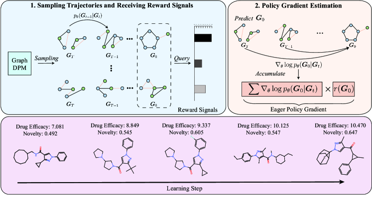
Figure 1: Overview of GDPO. (1) In each optimization step, GDPO samples multiple generation trajectories from the current Graph DPM and queries the reward function with different $\bm{G}_{0}$. (2) For each trajectory, GDPO accumulates the gradient $\nabla_{\theta}\log p_{\theta}(\bm{G}_{0}|\bm{G}_{t})$ of each $(\bm{G}_{0},\bm{G}_{t})$ pair and assigns a weight to the aggregated gradient based on the corresponding reward signal. Finally, GDPO estimates the eager policy gradient by averaging the aggregated gradient from all trajectories.

In this section, we study the problem of learning graph DPMs from arbitrary reward signals. We first present an MDP formulation of the problem and conduct an analysis on the failure of a straightforward application of REINFORCE. Based on the analysis, we introduce a substitute termed eager policy gradient, which forms the core of our proposed method Graph Diffusion Policy Optimization (GDPO).

4.1 A Markov Decision Process Formulation

A graph DPM defines a sample distribution $p_{\theta}(\bm{G}_{0})$ through its reverse denoising process $p_{\theta}(\bm{G}_{0:T})$. Given a reward signal $r(\cdot)$ defined on generated samples, we aim to maximize the expected reward (ER) over the sample distribution:

$$\mathcal{J}_{\textsc{ER}}(\theta)=\mathbb{E}_{\bm{G}_{0}\sim p_{\theta}(\bm{G}_{0})}\left[r(\bm{G}_{0})\right]\textrm{.}$$ (5)

However, directly optimizing $\mathcal{J}_{\textsc{ER}}(\theta)$ is challenging since the likelihood $p_{\theta}(\bm{G}_{0})$ is unavailable (Ho et al., 2020), hindering the use of typical RL algorithms (Black et al., 2023).

Following Fan et al. (2023), we formulate the denoising process as a $T$-step MDP and obtain an equivalent objective. Using notations in Sec. 3, the MDP is defined as follows:

$$\bm{s}_{t}\triangleq(\bm{G}_{T-t},T- t)\textrm{,}~{}~{}\bm{a}_{t}\triangleq\bm{G}_{T-t-1}\textrm{,}$$ (6)

$$\pi_{\theta}(\bm{a}_{t}|\bm{s}_{t})\triangleq p_{\theta}( \bm{G}_{T-t-1}|\bm{G}_{T-t})\textrm{,}$$

$$P(\bm{s}_{t+1}|\bm{s}_{t},\bm{a}_{t})\triangleq{}( \delta_{\bm{G}_{T-t-1}},\delta_{T-t-1})\textrm{,}$$

$$r(\bm{s}_{t},\bm{a}_{t})\triangleq r(\bm{G}_{0})\ \text{if}\ t={}T \textrm{,}~{}~{}~{}r(\bm{s}_{t},\bm{a}_{t})\triangleq 0\ \text{if}\ t<T\textrm{,}\!\!\!\!\!$$

where the initial state $\bm{s}_{0}$ corresponds to the initial noisy graph $\bm{G}_{T}$ of the denoising process and the policy corresponds to the reverse transition distribution. As a result, the graph generation trajectory $(\bm{G}_{T},\bm{G}_{T-1},\dots,\bm{G}_{0})$ can be considered as a state-action trajectory $\bm{\tau}$ produced by an agent acting in the MDP. It then follows that $p(\bm{\tau}|\pi_{\theta})=p_{\theta}(\bm{G}_{0:T})$. Moreover, we have $R(\bm{\tau})=\sum_{t=0}^{T}r(\bm{s}_{t},\bm{a}_{t})=r(\bm{G}_{0})$. Therefore, the expected cumulative reward of the agent $\mathcal{J}_{\textsc{RL}}(\theta)=\mathbb{E}_{p(\bm{\tau}|\pi_{\theta})}[R(\bm{\tau})]=\mathbb{E}_{p_{\theta}(\bm{G}_{0:T})}[r(\bm{G}_{0})]$ is equivalent to $\mathcal{J}_{\textsc{ER}}(\theta)$, and thus $\mathcal{J}_{\textsc{ER}}(\theta)$ can also be optimized with the policy gradient $\nabla_{\theta}\mathcal{J}_{\textsc{RL}}(\theta)$:

$$\nabla_{\theta}\mathcal{J}_{\textsc{RL}}(\theta)=\mathbb{E}_{\bm{\tau}}\left[r(\bm{G}_{0})\!\sum_{t=1}^{T}\nabla_{\theta}\log p_{\theta}(\bm{G}_{t-1}|\bm{G}_{t})\right]\textrm{,}$$ (7)

where the generation trajectory $\bm{\tau}$ follows $p_{\theta}(\bm{G}_{0:T})$.

4.2 Learning Graph DPMs with Policy Gradient

The policy gradient $\nabla_{\theta}\mathcal{J}_{\textsc{RL}}(\theta)$ in Eq. (7) is generally intractable and an efficient estimation is necessary. In a related setting centered on continuous-variable DPMs for image generation, DDPO (Black et al., 2023) estimates the policy gradient $\nabla_{\theta}\mathcal{J}_{\textsc{RL}}(\theta)$ with REINFORCE and achieves great results. This motivates us to also try REINFORCE on discrete-variable DPMs for graph generation, i.e., to approximate Eq. (7) with a Monte Carlo estimation:

$$\!\!\!\!\nabla_{\!\theta}\mathcal{J}_{\textsc{RL}}\!\approx\!\frac{1}{K}\!\!\sum_{k=1}^{K}\!\frac{T}{|\mathcal{T}_{k}|}\!\sum_{t\in\mathcal{T}_{k}}\!r(\bm{G}_{0}^{(k)})\nabla_{\!\theta}\!\log p_{\theta}(\bm{G}_{t-1}^{(k)}\!|\bm{G}_{t}^{(k)})\textrm{,}$$ (8)

where $\{\!\bm{G}_{0:T}^{(k)}\!\}_{k=1}^{K}$ are $K$ trajectories sampled from $p_{\theta}(\!\bm{G}_{0:T}\!)$ and $\{\mathcal{T}_{k}\subset[\![1,T]\!]\}_{k=1}^{K}$ are random subsets of timesteps.

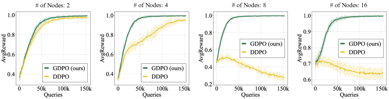
Figure 2: Toy experiment comparing DDPO and GDPO. We generate connected graphs with increasing number of nodes. Node categories are disregarded, and the edge categories are binary, indicating whether two nodes are linked. The graph DPM is initialized randomly as a one-layer graph transformer from DiGress (Vignac et al., 2022). The diffusion step $T$ is set to $50$, and the reward signal $r(\bm{G}_{0})$ is defined as $1$ if $\bm{G}_{0}$ is connected and $0$ otherwise. We use $256$ trajectories for gradient estimation in each update. The learning curve illustrates the diminishing performance of DDPO as the number of nodes increases, while GDPO consistently performs well.

However, we empirically observe that it rarely converges on graph DPMs. To investigate this, we design a toy experiment, where the reward signal is whether $\bm{G}_{0}$ is connected. The graph DPMs are randomly initialized and optimized using Eq. (8). We refer to this setting as DDPO. Fig. 2 depicts the learning curves, where the horizontal axis represents the number of queries to the reward signal and the vertical axis represents the average reward. The results demonstrate that DDPO fails to converge to a high reward signal area when generating graphs with more than 4 nodes. Furthermore, as the number of nodes increases, the fluctuation of the learning curves grows significantly. This implies that DDPO is essentially unable to optimize properly on randomly initialized models. We conjecture that the failure is due to the vast space constituted by discrete graph trajectories and the well-known high variance issue of REINFORCE (Sutton & Barto, 1998). A straightforward method to reduce variance is to sample more trajectories. However, this is typically expensive in DPMs, as each trajectory requires multiple rounds of model inference. Moreover, evaluating the reward signals of additional trajectories also incurs high computational costs, such as drug simulation (Pagadala et al., 2017).

Input: graph DPM $p_{\theta}$

Input: # of diffusion steps $T$, # of timestep samples $|\mathcal{T}|$

Input: reward signal $r(\cdot)$, # of trajectory samples $K$

Input: learning rate $\eta$ and # of training steps $N$

Output: Final graph DPM $p_{\theta}$

for $i=1,\dots,N$ do

     for $k=1,\dots,K$ do

         $\bm{G}_{0:T}^{(k)}\sim p_{\theta}$ // Sample trajectory

         $\mathcal{T}_{k}\sim\mathrm{Uniform}([\![1,T]\!])$ // Sample timesteps

         $r_{k}\leftarrow r(\bm{G}_{0}^{(k)})$ // Get rewards

        

     // Estimate reward mean and variance

     $\bar{r}\leftarrow\frac{1}{K}\sum_{k=1}^{K}r_{k}$  $\mathrm{std}[r]\leftarrow\sqrt{\frac{\sum_{k=1}^{K}(r_{k}-\bar{r})^{2}}{K-1}}$

     // Estimate the eager policy gradient

     $\bm{g}(\theta)\leftarrow\frac{1}{K}\sum\limits_{k=1}^{K}\!\frac{T}{|\mathcal{T}_{k}|}\!\sum\limits_{t\in\mathcal{T}_{k}}\!\!(\frac{r_{k}-\bar{r}}{\mathrm{std}[r]})\!\nabla_{\theta}\log p_{\theta}(\bm{G}_{0}^{(k)}|\bm{G}_{t}^{(k)})$

     // Update model parameter

     $\theta\leftarrow\theta+\eta\cdot\bm{g}(\theta)$

Algorithm 1 Graph Diffusion Policy Optimization

This prompts us to delve deeper at a micro level. Since the policy gradient estimation in Eq. (8) is a weighted summation of gradients, we first inspect each summand gradient term $\nabla_{\theta}\log p_{\theta}(\bm{G}_{t-1}|\bm{G}_{t})$. With the parameterization Eq. (1) described in Sec. 3.1, it has the following form:

$$~{}~{}\nabla_{\theta}\log p_{\theta}(\bm{G}_{t-1}|\bm{G}_{t})=$$

$$\frac{1}{p_{\theta}(\bm{G}_{t-1}|\bm{G}_{t})}\sum_{\widetilde{\bm{G}}_{0}}\leavevmode\color[rgb]{1,0,0}q(\bm{G}_{t-1}|\bm{G}_{t},\widetilde{\bm{G}}_{0})\leavevmode\color[rgb]{0,0,1}\nabla_{\theta}p_{\theta}(\widetilde{\bm{G}}_{0}|\bm{G}_{t})\textrm{,}$$ (9)

where we can view the red term as a weight assigned to the gradient $\leavevmode\color[rgb]{0,0,1}\nabla_{\theta}p_{\theta}(\widetilde{\bm{G}}_{0}|\bm{G}_{t})$, and thus $\nabla_{\theta}\log p_{\theta}(\bm{G}_{t-1}|\bm{G}_{t})$ as a weighted sum of such gradients, with $\widetilde{\bm{G}}_{0}$ taken over all possible graphs. Intuitively, the gradient $\leavevmode\color[rgb]{0,0,1}\nabla_{\theta}p_{\theta}(\widetilde{\bm{G}}_{0}|\bm{G}_{t})$ promotes the probability of predicting $\widetilde{\bm{G}}_{0}$ from $\bm{G}_{t}$. Note, however, that the weight $\leavevmode\color[rgb]{1,0,0}q(\bm{G}_{t-1}|\bm{G}_{t},\widetilde{\bm{G}}_{0})$ is completely independent of $r(\widetilde{\bm{G}}_{0})$ and could assign large weight for $\widetilde{\bm{G}}_{0}$ that has low reward. Since the weighted sum in Eq. (9) can be dominated by gradient terms with large $\leavevmode\color[rgb]{1,0,0}q(\bm{G}_{t-1}|\bm{G}_{t},\widetilde{\bm{G}}_{0})$, given a particular sampled trajectory, it is fairly possible that $\nabla_{\theta}\log p_{\theta}(\bm{G}_{t-1}|\bm{G}_{t})$ increases the probabilities of predicting undesired $\widetilde{\bm{G}}_{0}$ with low rewards from $\bm{G}_{t}$. This explains why Eq. (8) tends to produce fluctuating and unreliable policy gradient estimates when the number of Monte Carlo samples (i.e., $K$ and $|\mathcal{T}_{k}|$) is limited.

4.3 Graph Diffusion Policy Optimization

To address the above issues, we suggest a slight modification to Eq. (8) and obtain a new policy gradient denoted as $\bm{g}(\theta)$:

$$\!\bm{g}(\theta)\!\triangleq\!\frac{1}{K}\!\!\sum_{k=1}^{K}\!\frac{T}{|\mathcal{T}_{k}|}\!\sum_{t\in\mathcal{T}_{k}}\!r(\bm{G}_{0}^{(k)})\nabla_{\theta}\!\log p_{\theta}(\bm{G}_{0}^{(k)}\!|\bm{G}_{t}^{(k)})\textrm{,}$$ (10)

which we refer to as the eager policy gradient. Intuitively, although the number of possible graph trajectories is tremendous, if we partition them into different equivalence classes according to $\bm{G}_{0}$, where trajectories with the same $\bm{G}_{0}$ are considered equivalent, then the number of these equivalence classes will be much smaller than the number of graph trajectories. The optimization over these equivalence classes will be much easier than optimizing in the entire trajectory space.

Technically, by replacing the summand gradient term $\nabla_{\theta}\log p_{\theta}(\bm{G}_{t-1}|\bm{G}_{t})$ with $\nabla_{\theta}\log p_{\theta}(\bm{G}_{0}|\bm{G}_{t})$ in Eq. (8), we skip the weighted sum in Eq. (9) and directly promotes the probability of predicting $\bm{G}_{0}$ which has higher reward from $\bm{G}_{t}$ at all timestep $t$. As a result, our estimation does not focus on how $\bm{G}_{t}$ changes to $\bm{G}_{t-1}$ within the trajectory; instead, it aims to force the model’s generated results to be close to the desired $\bm{G}_{0}$, which can be seen as optimizing in equivalence classes. While being a biased estimator of the policy gradient $\nabla_{\theta}\mathcal{J}_{\textsc{RL}}(\theta)$, the eager policy gradient consistently leads to much less fluctuating learning and better performance than DDPO, as demonstrated in Fig. 2. We present the resulting method in Fig. 1 and Algorithm 1, naming it Graph Diffusion Policy Optimization (GDPO).

Table 1: General graph generation on SBM and Planar datasets.

Method	Planar Graphs					SBM Graphs
	Deg $\downarrow$	Clus $\downarrow$	Orb $\downarrow$	V.U.N (%) $\uparrow$		Deg $\downarrow$	Clus $\downarrow$	Orb $\downarrow$	V.U.N (%) $\uparrow$
GraphRNN	24.51 $\pm$ 3.22	9.03 $\pm$ 0.78	2508.30 $\pm$ 30.81	0		6.92 $\pm$ 1.13	1.72 $\pm$ 0.05	3.15 $\pm$ 0.23	4.92 $\pm$ 0.35
SPECTRE	2.55 $\pm$ 0.34	2.52 $\pm$ 0.26	2.42 $\pm$ 0.37	25.46 $\pm$ 1.33		1.92 $\pm$ 1.21	1.64 $\pm$ 0.06	1.67 $\pm$ 0.14	53.76 $\pm$ 3.62
GDSS	10.81 $\pm$ 0.86	12.99 $\pm$ 0.22	38.71 $\pm$ 0.83	0.78 $\pm$ 0.72		15.53 $\pm$ 1.30	3.50 $\pm$ 0.81	15.98 $\pm$ 2.30	0
MOOD	5.73 $\pm$ 0.82	11.87 $\pm$ 0.34	30.62 $\pm$ 0.67	1.21 $\pm$ 0.83		12.87$\pm$ 1.20	3.06 $\pm$ 0.37	2.81 $\pm$ 0.35	0
DiGress	1.43 $\pm$ 0.90	1.22 $\pm$ 0.32	1.72 $\pm$ 0.44	70.02 $\pm$ 2.17		1.63 $\pm$ 1.51	1.50 $\pm$ 0.04	1.70 $\pm$ 0.16	60.94 $\pm$ 4.98
DDPO	109.59$\pm$ 36.69	31.47 $\pm$ 4.96	504.19 $\pm$ 17.61	2.34 $\pm$ 1.10		250.06 $\pm$ 7.44	2.93 $\pm$ 0.32	6.65 $\pm$ 0.45	31.25 $\pm$ 5.22
GDPO (ours)	0.03 $\pm$ 0.04	0.62 $\pm$ 0.11	0.02 $\pm$ 0.01	73.83 $\pm$ 2.49		0.15 $\pm$ 0.13	1.50 $\pm$ 0.01	1.12 $\pm$ 0.14	80.08 $\pm$ 2.07

5 Reward Functions for Graph Generation

Graph data widely exists in different domains such as social network analysis (Freeman, 2004) and chemical research (Kearnes et al., 2016). In this work, we study both general graph and molecule-specific reward signals that are important in real-world downstream tasks. Due to the distinct properties desired in different generation tasks, reward signals can significantly vary in complexity and numerical range. Below, we elaborate on how we formulate diverse reward signals as numerical functions.

5.1 Reward Functions for General Graph Generation

Validity. For graph generation, a common objective is to generate a specific type of graph. For instance, one might be interested in graphs that can be drawn without edges crossing each other (Martinkus et al., 2022). For such objectives, the reward function $r_{\mathrm{val}}(\cdot)$ is then formulated as binary, with $r_{\mathrm{val}}(\bm{G}_{0})\triangleq 1$ indicating that the generated graph $\bm{G}_{0}$ conforms to the specified type; otherwise, $r_{\mathrm{val}}(\bm{G}_{0})\triangleq 0$.

Similarity. In certain scenarios, the objective is to generate graphs that resemble a known set of graphs $\mathcal{D}$ at the distribution level, based on a pre-defined distance metric $d(\cdot,\cdot)$ between sets of graphs. As an example, the $\textit{Deg}(\mathcal{G},\mathcal{D})$ (Liao et al., 2019a) measures the maximum mean discrepancy (MMD) (Gretton et al., 2012) between the degree distributions of a set $\mathcal{G}$ of generated graphs and the given graphs $\mathcal{D}$. Since our method requires a reward for each single generated graph $\bm{G}_{0}$, we simply adopt $\textit{Deg}(\{\bm{G}_{0}\},\mathcal{D})$ as the signal. As the magnitude of reward is critical for policy gradients (Sutton & Barto, 1998), we define $r_{\mathrm{deg}}(\bm{G}_{0})\triangleq\exp(-\textit{Deg}(\{\bm{G}_{0}\},\mathcal{D})^{2}/\sigma^{2})$, where the $\sigma$ controls the reward distribution, ensuring that the reward lies within the range of $0$ to $1$. The other two similar distance metrics are $\textit{Clus}(\mathcal{G},\mathcal{D})$ and $\textit{Orb}(\mathcal{G},\mathcal{D})$, which respectively measure the distances between two sets of graphs in terms of the distribution of clustering coefficients (Soffer & Vazquez, 2005) and the distribution of substructures (Ahmed et al., 2015). Based on the two metrics, we define two reward signals analogous to $r_{\mathrm{deg}}$, namely, $r_{\mathrm{clus}}$ and $r_{\mathrm{orb}}$.

5.2 Reward Functions for Molecular Graph Generation

Novelty. A primary objective of molecular graph generation is to discover novel drugs with desired therapeutic potentials. Due to drug patent restrictions, the novelty of generated molecules has paramount importance. The Tanimoto similarity (Bajusz et al., 2015), denoted as $J(\cdot,\cdot)$, measures the chemical similarity between two molecules, defined by the Jaccard index of molecule fingerprint bits. Specifically, $J\in[0,1]$, and $J(\bm{G}_{0},\bm{G}^{\prime}_{0})=1$ indicates that two molecules $\bm{G}_{0}$ and $\bm{G}^{\prime}_{0}$ have identical fingerprints. Following Xie et al. (2021), we define the novelty of a generated graph $\bm{G}_{0}$ as $\textit{NOV}(\bm{G}_{0})\triangleq 1-\max_{\bm{G}^{\prime}_{0}\in\mathcal{D}}J(\bm{G}_{0},\bm{G}^{\prime}_{0})$, i.e., the similarity gap between $\bm{G}_{0}$ and its nearest neighbor in the training dataset $\mathcal{D}$, and further define $r_{\textsc{nov}}(\bm{G}_{0})\triangleq\textit{NOV}(\bm{G}_{0})$.

Drug-Likeness. Regarding the efficacy of molecular graph generation in drug design, a critical indicator is the binding affinity between the generated drug candidate and a target protein. The docking score (Ciepliński et al., 2020), denoted as $\textit{DS}(\cdot)$, estimates the binding energy (in kcal/mol) between the ligand and the target protein through physical simulations in 3D space. Following Lee et al. (2022), we clip the docking score in the range $[-20,0]$ and define the reward function as $r_{\textsc{ds}}(\bm{G}_{0})\triangleq-\textit{DS}(\bm{G}_{0})/20$.

Another metric is the quantitative estimate of drug-likeness $\textit{QED}(\cdot)$, which measures the chemical properties to gauge the likelihood of a molecule being a successful drug (Bickerton et al., 2012). As it takes values in the range $[0,1]$, we adopt $r_{\textsc{qed}}(\bm{G}_{0})\triangleq\mathbb{I}[\textit{QED}(\bm{G}_{0})>0.5]$.

Synthetic Accessibility. The synthetic accessibility (Boda et al., 2007) $\textit{SA}(\cdot)$ evaluates the inherent difficulty in synthesizing a chemical compound, with values in the range from $1$ to $10$. We follow Lee et al. (2022) and use a normalized version as the reward function: $r_{\textsc{sa}}(\bm{G}_{0})\triangleq(10-\textit{SA}(\bm{G}_{0}))/9$.

Table 2: Molecule property optimization results on ZINC250k.

Method	Metric	Target Protein
		parp1	fa7	5ht1b	braf	jak2
REINVENT	Hit Ratio	0.480 $\pm$ 0.344	0.213 $\pm$ 0.081	2.453 $\pm$ 0.561	0.127 $\pm$ 0.088	0.613 $\pm$ 0.167
	DS (top $5\%$)	-8.702 $\pm$ 0.523	-7.205 $\pm$ 0.264	-8.770 $\pm$ 0.316	-8.392 $\pm$ 0.400	-8.165 $\pm$ 0.277
HierVAE	Hit Ratio	0.553 $\pm$ 0.214	0.007 $\pm$ 0.013	0.507 $\pm$ 0.278	0.207 $\pm$ 0.220	0.227 $\pm$ 0.127
	DS (top $5\%$)	-9.487 $\pm$ 0.278	-6.812 $\pm$ 0.165	-8.081 $\pm$ 0.252	-8.978 $\pm$ 0.525	-8.285 $\pm$ 0.370
FREED	Hit Ratio	4.627 $\pm$ 0.727	1.332 $\pm$ 0.113	16.767 $\pm$ 0.897	2.940 $\pm$ 0.359	5.800 $\pm$ 0.295
	DS (top $5\%$)	-10.579 $\pm$ 0.104	-8.378 $\pm$ 0.044	-10.714 $\pm$ 0.183	-10.561 $\pm$ 0.080	-9.735 $\pm$ 0.022
MOOD	Hit Ratio	7.017 $\pm$ 0.428	0.733 $\pm$ 0.141	18.673 $\pm$ 0.423	5.240 $\pm$ 0.285	9.200 $\pm$ 0.524
	DS (top $5\%$)	-10.865 $\pm$ 0.113	-8.160 $\pm$ 0.071	-11.145 $\pm$ 0.042	-11.063 $\pm$ 0.034	-10.147 $\pm$ 0.060
DiGress	Hit Ratio	0.366 $\pm$ 0.146	0.182 $\pm$ 0.232	4.236 $\pm$ 0.887	0.122 $\pm$ 0.141	0.861 $\pm$ 0.332
	DS (top $5\%$)	-9.219 $\pm$ 0.078	-7.736 $\pm$ 0.156	-9.280 $\pm$ 0.198	-9.052 $\pm$ 0.044	-8.706 $\pm$ 0.222
DDPO	Hit Ratio	0.419 $\pm$ 0.280	0.342 $\pm$ 0.685	5.488 $\pm$ 1.989	0.445 $\pm$ 0.297	1.717 $\pm$ 0.684
	DS (top $5\%$)	-9.247 $\pm$ 0.242	-7.739 $\pm$ 0.244	-9.488 $\pm$ 0.287	-9.470 $\pm$ 0.373	-8.990 $\pm$ 0.221
GDPO (ours)	Hit Ratio	9.814 $\pm$ 1.352	3.449 $\pm$ 0.188	34.359 $\pm$ 2.734	9.039 $\pm$ 1.473	13.405 $\pm$ 1.515
	DS (top $5\%$)	-10.938 $\pm$ 0.042	-8.691 $\pm$ 0.074	-11.304 $\pm$ 0.093	-11.197 $\pm$ 0.132	-10.183 $\pm$ 0.124

6 Experiments

In this section, we first examine the performance of GDPO on both general graph generation tasks and molecular graph generation tasks. Then, we conduct several ablation studies to investigate the effectiveness of GDPO’s design.

6.1 General Graph Generation

Datasets and Baselines. Following DiGress (Vignac et al., 2022), we evaluate GDPO on two benchmark datasets: SBM (200 nodes) and Planar (64 nodes), each consisting of 200 graphs. We compare GDPO with GraphRNN (You et al., 2018b), SPECTRE (Martinkus et al., 2022), GDSS (Jo et al., 2022), MOOD (Lee et al., 2022) and DiGress. The first two models are based on RNN and GAN, respectively. The remaining methods are all graph DPMs, and MOOD employs an additional property predictor. We also test DDPO (Black et al., 2023), i.e., graph DPMs optimized with Eq. (8).

Implementation. We set $T=1000$, $|\mathcal{T}|=200$, and $N=100$. The number of trajectory samples $K$ is $64$ for SBM and $256$ for Planar. We use a DiGress model with $10$ layers. More implementation details can be found in Appendix A.

Metrics and Reward Functions. We consider four metrics: $\textit{Deg}(\mathcal{G},\mathcal{D}_{test})$, $\textit{Clus}(\mathcal{G},\mathcal{D}_{test})$, $\textit{Orb}(\mathcal{G},\mathcal{D}_{test})$, and the V.U.N metrics. V.U.N measures the proportion of generated graphs that are valid, unique, and novel. The reward function is defined as follows:

$$r_{\mathrm{general}}=0.1\times(r_{\mathrm{deg}}+r_{\mathrm{clus}}+r_{\mathrm{orb}})+0.7\times r_{\mathrm{val}}\textrm{,}$$ (11)

where we do not explicitly incorporate uniqueness and novelty in to the reward. All rewards are calculated on the training dataset if a reference graph set is required. All evaluation metrics are calculated on the test dataset. More details about baselines, reward signals, and metrics are in Appendix A.1.

Results. Table 1 summarizes GDPO’s superior performance in general graph generation, showing notable improvements in Deg and V.U.N across both SBM and Planar datasets. On the Planar dataset, GDPO significantly reduces distribution distance, achieving an $\mathbf{81.97\%}$ average decrease in metrics of Deg, Clus, and Orb compared to DiGress (the best baseline method). For the SBM dataset, GDPO has a $\mathbf{41.64\%}$ average improvement. The low distributional distances to the test dataset suggests that GDPO accurately captures the data distribution with well-designed rewards. Moreover, we observe that our method outperforms DDPO by a large margin, primarily because the graphs in Planar and SBM contain too many nodes, which aligns with the observation in Fig. 2.

Table 3: Molecule Dataset Statistics.

Dataset	Molecules	Atom Types	Max Atoms
ZINC250k	249,456	9	38
MOSES	1,584,663	8	30

Table 4: Molecule property optimization results on MOSES.

Method	Metric	Target Protein
		parp1	fa7	5ht1b	braf	jak2
FREED	Hit Ratio	0.532 $\pm$ 0.614	0	4.255 $\pm$ 0.869	0.263 $\pm$ 0.532	0.798 $\pm$ 0.532
	DS (top $5\%$)	-9.313 $\pm$ 0.357	-7.825 $\pm$ 0.167	-9.506 $\pm$ 0.236	-9.306 $\pm$ 0.327	-8.594 $\pm$ 0.240
MOOD	Hit Ratio	5.402 $\pm$ 0.042	0.365 $\pm$ 0.200	26.143 $\pm$ 1.647	3.932 $\pm$ 1.290	11.301 $\pm$ 1.154
	DS (top $5\%$)	-9.814 $\pm$ 1.352	-7.974 $\pm$ 0.029	10.734 $\pm$ 0.049	-10.722 $\pm$ 0.135	-10.158 $\pm$ 0.185
DiGress	Hit Ratio	0.231 $\pm$ 0.463	0.113 $\pm$ 0.131	3.852 $\pm$ 5.013	0	0.228 $\pm$ 0.457
	DS (top $5\%$)	-9.223 $\pm$ 0.083	-6.644 $\pm$ 0.533	-8.640 $\pm$ 0.907	8.522 $\pm$ 1.017	-7.424 $\pm$ 0.994
DDPO	Hit Ratio	3.037 $\pm$ 2.107	0.504 $\pm$ 0.667	7.855 $\pm$ 1.745	0	3.943 $\pm$ 2.204
	DS (top $5\%$)	-9.727 $\pm$ 0.529	-8.025 $\pm$ 0.253	-9.631 $\pm$ 0.123	-9.407 $\pm$ 0.125	-9.404 $\pm$ 0.319
GDPO (ours)	Hit Ratio	24.711 $\pm$ 1.775	1.393 $\pm$ 0.982	17.646 $\pm$ 2.484	19.968 $\pm$ 2.309	26.688 $\pm$ 2.401
	DS (top $5\%$)	-11.002 $\pm$ 0.056	-8.468 $\pm$ 0.058	-10.990 $\pm$ 0.334	-11.337 $\pm$ 0.137	-10.290 $\pm$ 0.069

6.2 Molecule Property Optimization

Datasets and Baselines. Molecule property optimization aims to generate molecules with desired properties. We evaluate our method on two large molecule datasets: ZINC250k (Irwin et al., 2012) and MOSES (Polykovskiy et al., 2018). Data statistics are presented in Table 3. We compare GDPO with several leading methods: REINVENT (Olivecrona et al., 2017), HierVAE (Jin et al., 2020a), FREED (Yang et al., 2021) and MOOD (Lee et al., 2022). REINVENT and FREED are RL methods that search in the chemical environment. HierVAE uses a VAE for hierarchical motif-based molecule generation. MOOD, based on graph DPMs, employs a property predictor for guided sampling. Similar to general graph generation, we also compare our method with DiGress and DDPO.

Implementation. We set $T=500$, $|\mathcal{T}|=100$, $N=100$, and $K=256$ for both datasets. We use the same model structure with DiGress. See more details in Appendix A.

Metrics and Reward Functions. Following MOOD, we consider two metrics essential for real-world novel drug discovery: Novel hit ratio (%) and Novel top $5\%$ docking score, denoted as Hit Ratio and DS (top $5\%$), respectively. Using the notations from Sec. 5.2, the Hit Ratio is the proportion of unique generated molecules that satisfy: DS $<$ median DS of the known effective molecules, NOV $>$ 0.6, QED $>$ 0.5, and SA$\ <$ 5. The DS (top $5\%$) is the average DS of the top $5\%$ molecules (ranked by DS) that satisfy: NOV $>$ 0.6, QED $>$ 0.5, and SA$\ <$ 5. Since calculating DS requires specifying a target protein, we set five different protein targets to fully test GDPO: parp1, fa7, 5ht1b, braf, and jak2. The reward function for molecule property optimization is defined as follows:

$$r_{\mathrm{molecule}}=0.1\times(r_{\textsc{qed}}+r_{\textsc{sa}})+0.3\times r_{\textsc{nov}}+0.5\times r_{\textsc{ds}}\textrm{.}$$ (12)

We do not directly use Hit Ratio and DS (top $5\%$) as rewards in consideration of method generality. The reward weights are determined through several rounds of search, and we find that assigning a high weight to $r_{\textsc{nov}}$ leads to training instability, which is discussed in Sec. 6.3. More details about the experiment settings are discussed in Appendix A.2.

Results. In Table 2, GDPO shows significant improvement on ZINC250k, especially in the Hit Ratio. A higher Hit Ratio means the model is more likely to generate valuable new drugs, and GDPO averagely improves the Hit Ratio by $5.72\%$ in comparison with other SOTA methods. For DS (top $5\%$), GDPO also has a $1.48\%$ improvement on average. Discovering new drugs on MOSES is much more challenging than on ZINC250k due to its vast training dataset. In Table 4, GDPO also shows promising results on MOSES. Despite a less favorable Hit Ratio on 5ht1b, GDPO achieves an average improvement of $12.94\%$ on the other four target proteins. For DS (top $5\%$), GDPO records an average improvement of $5.54\%$ compared to MOOD, indicating a significant enhancement in the drug efficacy of the generated samples.

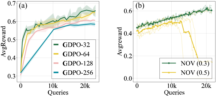
Figure 3: We investigate two key factors of GDPO on ZINC250k, with the target protein being 5ht1b. Similarly, the vertical axis represents the total queries, while the horizontal axis represents the average reward.(a) We vary the number of trajectories for gradient estimation. (b) We fix the weight of $r_{\textsc{QED}}$ and $r_{\textsc{SA}}$, and change the weight of $r_{\textsc{NOV}}$ while ensuring the total weight is 1.

6.3 Sample Efficiency and Novelty Optimization

We investigate two crucial factors for GDPO: the first one is the number of trajectories for gradient estimation, and the second one is the selection of the reward function. We test our method on ZINC250k and set the target proteins as 5ht1b. In Fig. 3 (a), the results indicate that GDPO exhibits good sampling efficiency, as it achieves a significant improvement in average reward by querying only 10k molecule reward signals, which is much less than the number of molecules contained in ZINC250k. Furthermore, the sample efficiency of GDPO can be further enhanced by reducing the number of trajectories, but this may lead to training instability. To achieve consistent improvements across multiple target proteins, we use 256 trajectories for gradient estimation in our experiments. In Fig. 3 (b), we demonstrate a failure case of GDPO when assigning a high weight to $r_{\textsc{NOV}}$. For generative models, generating a sample that is completely different from the training set is challenging. MOOD (Lee et al., 2022) achieves this by adding noise during the sampling process, while we achieve it by directly optimizing the novelty. However, assigning a large weight to $r_{\textsc{NOV}}$ can lead the model to degenerate rapidly. One possible solution is to gradually increase the weight and conduct multi-stage optimization.

7 Conclusion

We introduce GDPO, a novel policy gradient method for learning graph DPMs that effectively addresses the problem of graph generation under given objectives. Evaluation results on both general and molecular graphs indicate that GDPO is compatible with complex multi-objective optimization and achieves state-of-the-art performance on a series of representative graph generation tasks. Our future work will investigate the theoretical gap between GDPO and DDPO in order to obtain effective unbiased estimators.

Impact Statements

This paper presents work whose goal is to advance the field of Machine Learning. There are many potential societal consequences of our work, none which we feel must be specifically highlighted here.

Appendix A Experimental Details and Additional Results

Table 5: General graph generation on SBM and Planar datasets.

Method	Planar Graphs
	Deg $\downarrow$	Clus $\downarrow$	Orb $\downarrow$	V.U.N (%) $\uparrow$
Validity (0.6)	0.03 $\pm$ 0.03	0.54 $\pm$ 0.08	0.02 $\pm$ 0.01	72.34 $\pm$ 2.78
Validity (0.7)	0.03 $\pm$ 0.04	0.62 $\pm$ 0.11	0.02 $\pm$ 0.01	73.83$\pm$ 2.49
Validity (0.8)	0.12 $\pm$ 0.04	0.88 $\pm$ 0.34	0.24 $\pm$ 0.07	78.68 $\pm$ 3.12
Validity (0.9)	0.86 $\pm$ 0.12	2.17 $\pm$ 0.84	1.46 $\pm$ 0.78	81.26 $\pm$ 3.02

Implementation Details. For all experiments, we use the graph transformer proposed in DiGress (Vignac et al., 2022) as the graph DPMs, and the models are pre-trained on the training dataset before applying GDPO or DDPO. During fine-tuning, we keep all layers fixed except for attention, set the learning rate to 0.00001, and utilize gradient clipping to limit the gradient norm to be less than or equal to 1. In addition, due to significant numerical fluctuations during reward normalization, we follow DDPO (Black et al., 2023) in constraining the normalized reward to the range from $[-5,5]$. This means that gradients resulting from rewards beyond this range will not contribute to model updates. When there is insufficient memory to generate enough trajectories, we use gradient accumulation to increase the number of trajectories used for gradient estimation. We conducted all experiments on a single A100 GPU with 40GB of VRAM and an AMD EPYC 7352 24-core Processor.

A.1 General Graph Generation

Baselines. There are several baseline methods for general graph generation, we summarize them as follows:

• GraphRNN: a deep autoregressive model designed to model and generate complex distributions over graphs. It addresses challenges like non-uniqueness and high dimensionality by decomposing the generation process into node and edge formations.

• SPECTRE: a novel GAN for graph generation, approaches the problem spectrally by generating dominant parts of the graph Laplacian spectrum and matching them to eigenvalues and eigenvectors. This method allows for modeling global and local graph structures directly, overcoming issues like expressivity and mode collapse.

• GDSS: A novel score-based generative model for graphs is introduced to tackle the task of capturing permutation invariance and intricate node-edge dependencies in graph data generation. This model employs a continuous-time framework incorporating a novel graph diffusion process, characterized by stochastic differential equations (SDEs), to simultaneously model distributions of nodes and edges.

• DiGress: DiGress is a discrete denoising diffusion model designed for generating graphs with categorical attributes for nodes and edges. It employs a discrete diffusion process to iteratively modify graphs with noise, guided by a graph transformer network. By preserving the distribution of node and edge types and incorporating graph-theoretic features, DiGress achieves state-of-the-art performance on various datasets.

• MOOD: MOOD introduces Molecular Out-Of-distribution Diffusion, which employs out-of-distribution control in the generative process without added costs. By incorporating gradients from a property predictor, MOOD guides the generation process towards molecules with desired properties, enabling the discovery of novel and valuable compounds surpassing existing methods

Metrics. The metrics of general graph generations are all taken from GraphRNN (Liao et al., 2019a). The reported metrics compare the discrepancy between the distribution of certain metrics on a test set and the distribution of the same metrics on a generated graph. The metrics measured include degree distributions, clustering coefficients, and orbit counts (which measure the distribution of all substructures of size 4). Following DiGress (Vignac et al., 2022), we do not report raw numbers but ratios computed as follows:

$$r=\operatorname{MMD}(\textit{generated},\textit{test})^{2}/\operatorname{MMD}(\textit{training},\textit{test})^{2}$$ (13)

Besides, we explain some metrics that are used in the general graph generation:

• Clus: the clustering coefficient measures the tendency of nodes to form clusters in a network. Real-world networks, especially social networks, often exhibit tightly knit groups with more ties between nodes than expected by chance. There are two versions of this measure: global, which assesses overall clustering in the network, and local, which evaluates the clustering around individual nodes.

• Orb: Graphlets are induced subgraph isomorphism classes in a graph, where occurrences are isomorphic or non-isomorphic. They differ from network motifs, which are over- or under-represented graphlets compared to a random graph null model. Orb will count the occurrences of each type of graphlet in a graph. Generally, if two graphs have similar numbers of graphlets, they are considered to be relatively similar.

Reward Signals. We showcase the performance of GDPO on Planar under different configurations of reward weights. We keep the three weights related to distance the same and adjust the weight of validity while ensuring that the sum of weights is 1. The results indicate that GDPO is not very sensitive to the weights of several reward signals for general graph generation, even though these weight configurations vary significantly, they all achieve good performance. Additionally, we found that GDPO can easily increase V.U.N to above 80 while experiencing slight losses in the other three indicators. When applying GDPO in practice, one can make a tradeoff between them based on the specific application requirements.

A.2 Molecule Property Optimization

Implementation Details. Following FREED (Yang et al., 2021), we selected five proteins, PARP-1 (Poly [ADP-ribose] polymerase-1), FA7 (Coagulation factor VII), 5-HT1B (5-hydroxytryptamine receptor 1B), BRAF (Serine/threonine-protein kinase B-raf), and JAK2 (Tyrosine-protein kinase JAK2), which have the highest AUROC scores when the protein-ligand binding affinities for DUD-E ligands are approximated with AutoDock Vina (Eberhardt et al., 2021), as the target proteins for which the docking scores are calculated. QED and SA scores are computed using the RDKit library.

Baselines. There are several baseline methods for molecular graph generation under the given objectives, they are diverse in methodology and performance, we summarize them as follows:

• REINVENT: This method enhances a sequence-based generative model for molecular design by incorporating augmented episodic likelihood, enabling the generation of structures with specified properties. It successfully performs tasks such as generating analogs to a reference molecule and predicting compounds active against a specific biological target.

• HierVAE: a hierarchical graph encoder-decoder for drug discovery, overcoming limitations of previous approaches by using larger and more flexible graph motifs as building blocks. The encoder generates a multi-resolution representation of molecules, while the decoder adds motifs in a coarse-to-fine manner, effectively resolving attachments to the molecule.

• FREED: a novel reinforcement learning (RL) framework for generating effective acceptable molecules with high docking scores, crucial for drug design. FREED addresses challenges in generating realistic molecules and optimizing docking scores through a fragment-based generation method and error-prioritized experience replay (PER).

• MOOD: please refer to Appendix A.1.

Metrics. There are several metrics for evaluating the molecule properties, we summarize the meaning of these metrics as follows:

• Docking Score: Docking simulations aim to find the best binding mode based on scoring functions. Scoring functions in computational chemistry and molecular modeling predict binding affinity between molecules post-docking. They are commonly used for drug-protein interactions, but also for protein-protein or protein-DNA interactions. After defining the score function, we can optimize to find the optimal drug-protein matching positions and obtain the docking score.

• QED: Drug-likeness evaluation in drug discovery often lacks nuance, leading to potential issues with compound quality. We introduce QED, a measure based on desirability, which considers the distribution of molecular properties and allows the ranking of compounds by relative merit. QED is intuitive, transparent, and applicable to various settings. We extend its use to assess molecular target druggability and suggest it may reflect aesthetic considerations in medicinal chemistry.

• SA: a scoring method for rapid evaluation of synthetic accessibility, considering structural complexity, similarity to available starting materials, and strategic bond assessments. These components are combined using an additive scheme, with weights determined via linear regression analysis based on medicinal chemists’ accessibility scores. The calculated synthetic accessibility values align well with chemists’ assessments.

References

- Ahmed et al. (2015) Ahmed, N. K., Neville, J., Rossi, R. A., and Duffield, N. Efficient graphlet counting for large networks. In 2015 IEEE international conference on data mining, pp. 1–10. IEEE, 2015.
- Austin et al. (2021) Austin, J., Johnson, D. D., Ho, J., Tarlow, D., and van den Berg, R. Structured denoising diffusion models in discrete state-spaces. ArXiv, abs/2107.03006, 2021.
- Bai et al. (2022) Bai, Y., Jones, A., Ndousse, K., Askell, A., Chen, A., DasSarma, N., Drain, D., Fort, S., Ganguli, D., Henighan, T. J., Joseph, N., Kadavath, S., Kernion, J., Conerly, T., El-Showk, S., Elhage, N., Hatfield-Dodds, Z., Hernandez, D., Hume, T., Johnston, S., Kravec, S., Lovitt, L., Nanda, N., Olsson, C., Amodei, D., Brown, T. B., Clark, J., McCandlish, S., Olah, C., Mann, B., and Kaplan, J. Training a helpful and harmless assistant with reinforcement learning from human feedback. ArXiv, abs/2204.05862, 2022.
- Bajusz et al. (2015) Bajusz, D., Rácz, A., and Héberger, K. Why is tanimoto index an appropriate choice for fingerprint-based similarity calculations? Journal of Cheminformatics, 7, 2015.
- Bickerton et al. (2012) Bickerton, G. R. J., Paolini, G. V., Besnard, J., Muresan, S., and Hopkins, A. L. Quantifying the chemical beauty of drugs. Nature chemistry, 4 2:90–8, 2012.
- Black et al. (2023) Black, K., Janner, M., Du, Y., Kostrikov, I., and Levine, S. Training diffusion models with reinforcement learning. ArXiv, abs/2305.13301, 2023.
- Blaschke et al. (2020) Blaschke, T., Engkvist, O., Bajorath, J., and Chen, H. Memory-assisted reinforcement learning for diverse molecular de novo design. Journal of Cheminformatics, 12, 2020.
- Boda et al. (2007) Boda, K., Seidel, T., and Gasteiger, J. Structure and reaction based evaluation of synthetic accessibility. Journal of Computer-Aided Molecular Design, 21:311–325, 2007.
- Brockschmidt et al. (2018) Brockschmidt, M., Allamanis, M., Gaunt, A. L., and Polozov, O. Generative code modeling with graphs. ArXiv, abs/1805.08490, 2018.
- Cao & Kipf (2018) Cao, N. D. and Kipf, T. Molgan: An implicit generative model for small molecular graphs. ArXiv, abs/1805.11973, 2018.
- Ciepliński et al. (2020) Ciepliński, T., Danel, T., Podlewska, S., and Jastrzebski, S. Generative models should at least be able to design molecules that dock well: A new benchmark. Journal of Chemical Information and Modeling, 63:3238 – 3247, 2020.
- Clark et al. (2023) Clark, K., Vicol, P., Swersky, K., and Fleet, D. J. Directly fine-tuning diffusion models on differentiable rewards. ArXiv, abs/2309.17400, 2023.
- Dhariwal & Nichol (2021) Dhariwal, P. and Nichol, A. Diffusion models beat gans on image synthesis. ArXiv, abs/2105.05233, 2021.
- Eberhardt et al. (2021) Eberhardt, J., Santos-Martins, D., Tillack, A. F., and Forli, S. Autodock vina 1.2. 0: New docking methods, expanded force field, and python bindings. Journal of chemical information and modeling, 61(8):3891–3898, 2021.
- Eckmann et al. (2022) Eckmann, P., Sun, K., Zhao, B., Feng, M., Gilson, M. K., and Yu, R. Limo: Latent inceptionism for targeted molecule generation. Proceedings of machine learning research, 162:5777–5792, 2022.
- Erdos & Rényi (1984) Erdos, P. L. and Rényi, A. On the evolution of random graphs. Transactions of the American Mathematical Society, 286:257–257, 1984.
- Fan & Lee (2023) Fan, Y. and Lee, K. Optimizing ddpm sampling with shortcut fine-tuning. In International Conference on Machine Learning, 2023.
- Fan et al. (2023) Fan, Y., Watkins, O., Du, Y., Liu, H., Ryu, M., Boutilier, C., Abbeel, P., Ghavamzadeh, M., Lee, K., and Lee, K. Dpok: Reinforcement learning for fine-tuning text-to-image diffusion models. ArXiv, abs/2305.16381, 2023.
- Feinberg & Shwartz (2012) Feinberg, E. A. and Shwartz, A. Handbook of Markov decision processes: methods and applications, volume 40. Springer Science & Business Media, 2012.
- Freeman (2004) Freeman, L. The development of social network analysis. A Study in the Sociology of Science, 1(687):159–167, 2004.
- Gretton et al. (2012) Gretton, A., Borgwardt, K. M., Rasch, M. J., Scholkopf, B., and Smola, A. A kernel two-sample test. J. Mach. Learn. Res., 13:723–773, 2012.
- Grondman et al. (2012) Grondman, I., Busoniu, L., Lopes, G. A., and Babuska, R. A survey of actor-critic reinforcement learning: Standard and natural policy gradients. IEEE Transactions on Systems, Man, and Cybernetics, Part C (Applications and Reviews), 42(6):1291–1307, 2012.
- Grover et al. (2018) Grover, A., Zweig, A., and Ermon, S. Graphite: Iterative generative modeling of graphs. In International Conference on Machine Learning, 2018.
- Guo & Zhao (2020) Guo, X. and Zhao, L. A systematic survey on deep generative models for graph generation. IEEE Transactions on Pattern Analysis and Machine Intelligence, 45:5370–5390, 2020.
- Harary & Nash-Williams (1965) Harary, F. and Nash-Williams, C. S. J. A. On eulerian and hamiltonian graphs and line graphs. Canadian Mathematical Bulletin, 8:701 – 709, 1965.
- Hasanzadeh et al. (2019) Hasanzadeh, A., Hajiramezanali, E., Duffield, N. G., Narayanan, K. R., Zhou, M., and Qian, X. Semi-implicit graph variational auto-encoders. ArXiv, abs/1908.07078, 2019.
- Ho et al. (2020) Ho, J., Jain, A., and Abbeel, P. Denoising diffusion probabilistic models. ArXiv, abs/2006.11239, 2020.
- Holland et al. (1983) Holland, P., Laskey, K. B., and Leinhardt, S. Stochastic blockmodels: First steps. Social Networks, 5:109–137, 1983.
- Irwin et al. (2012) Irwin, J. J., Sterling, T., Mysinger, M. M., Bolstad, E. S., and Coleman, R. G. Zinc: A free tool to discover chemistry for biology. Journal of Chemical Information and Modeling, 52:1757 – 1768, 2012.
- Jeon & Kim (2020) Jeon, W. and Kim, D. Autonomous molecule generation using reinforcement learning and docking to develop potential novel inhibitors. Scientific Reports, 10, 2020.
- Jin et al. (2020a) Jin, W., Barzilay, R., and Jaakkola, T. Hierarchical generation of molecular graphs using structural motifs. In International Conference on Machine Learning, 2020a.
- Jin et al. (2020b) Jin, W., Barzilay, R., and Jaakkola, T. Multi-objective molecule generation using interpretable substructures. In International Conference on Machine Learning, 2020b.
- Jo et al. (2022) Jo, J., Lee, S., and Hwang, S. J. Score-based generative modeling of graphs via the system of stochastic differential equations. In International Conference on Machine Learning, 2022.
- Karras et al. (2022) Karras, T., Aittala, M., Aila, T., and Laine, S. Elucidating the design space of diffusion-based generative models. ArXiv, abs/2206.00364, 2022.
- Kearnes et al. (2016) Kearnes, S., McCloskey, K., Berndl, M., Pande, V., and Riley, P. Molecular graph convolutions: moving beyond fingerprints. Journal of computer-aided molecular design, 30:595–608, 2016.
- Kinnings et al. (2011) Kinnings, S. L., Liu, N., Tonge, P. J., Jackson, R. M., Xie, L., and Bourne, P. E. A machine learning-based method to improve docking scoring functions and its application to drug repurposing. Journal of chemical information and modeling, 51 2:408–19, 2011.
- Kipf & Welling (2016) Kipf, T. and Welling, M. Variational graph auto-encoders. ArXiv, abs/1611.07308, 2016.
- Lee et al. (2023) Lee, K., Liu, H., Ryu, M., Watkins, O., Du, Y., Boutilier, C., Abbeel, P., Ghavamzadeh, M., and Gu, S. S. Aligning text-to-image models using human feedback. ArXiv, abs/2302.12192, 2023.
- Lee & Min (2022) Lee, M.-S. and Min, K. Mgcvae: Multi-objective inverse design via molecular graph conditional variational autoencoder. Journal of chemical information and modeling, 2022.
- Lee et al. (2022) Lee, S., Jo, J., and Hwang, S. J. Exploring chemical space with score-based out-of-distribution generation. ArXiv, abs/2206.07632, 2022.
- Liao et al. (2019a) Liao, R., Li, Y., Song, Y., Wang, S., Hamilton, W., Duvenaud, D. K., Urtasun, R., and Zemel, R. Efficient graph generation with graph recurrent attention networks. Advances in neural information processing systems, 32, 2019a.
- Liao et al. (2019b) Liao, R., Li, Y., Song, Y., Wang, S., Nash, C., Hamilton, W. L., Duvenaud, D. K., Urtasun, R., and Zemel, R. S. Efficient graph generation with graph recurrent attention networks. In Neural Information Processing Systems, 2019b.
- Liu et al. (2019) Liu, J., Kumar, A., Ba, J., Kiros, J. R., and Swersky, K. Graph normalizing flows. ArXiv, abs/1905.13177, 2019.
- Liu et al. (2018) Liu, Q., Allamanis, M., Brockschmidt, M., and Gaunt, A. L. Constrained graph variational autoencoders for molecule design. In Neural Information Processing Systems, 2018.
- Luo et al. (2021) Luo, Y., Yan, K., and Ji, S. Graphdf: A discrete flow model for molecular graph generation. In International Conference on Machine Learning, 2021.
- Martinkus et al. (2022) Martinkus, K., Loukas, A., Perraudin, N., and Wattenhofer, R. Spectre : Spectral conditioning helps to overcome the expressivity limits of one-shot graph generators. In International Conference on Machine Learning, 2022.
- Nguyen & Wei (2019) Nguyen, D. D. and Wei, G. Agl-score: Algebraic graph learning score for protein-ligand binding scoring, ranking, docking, and screening. Journal of chemical information and modeling, 2019.
- Nguyen et al. (2017) Nguyen, K., Daumé, H., and Boyd-Graber, J. L. Reinforcement learning for bandit neural machine translation with simulated human feedback. ArXiv, abs/1707.07402, 2017.
- Niu et al. (2020) Niu, C., Song, Y., Song, J., Zhao, S., Grover, A., and Ermon, S. Permutation invariant graph generation via score-based generative modeling. In International Conference on Artificial Intelligence and Statistics, 2020.
- Olivecrona et al. (2017) Olivecrona, M., Blaschke, T., Engkvist, O., and Chen, H. Molecular de-novo design through deep reinforcement learning. Journal of Cheminformatics, 9, 2017.
- Pagadala et al. (2017) Pagadala, N. S., Syed, K., and Tuszynski, J. A. Software for molecular docking: a review. Biophysical Reviews, 9:91 – 102, 2017.
- Polykovskiy et al. (2018) Polykovskiy, D., Zhebrak, A., Sánchez-Lengeling, B., Golovanov, S., Tatanov, O., Belyaev, S., Kurbanov, R., Artamonov, A. A., Aladinskiy, V., Veselov, M., Kadurin, A., Nikolenko, S. I., Aspuru-Guzik, A., and Zhavoronkov, A. Molecular sets (moses): A benchmarking platform for molecular generation models. Frontiers in Pharmacology, 11, 2018.
- Prabhudesai et al. (2023) Prabhudesai, M., Goyal, A., Pathak, D., and Fragkiadaki, K. Aligning text-to-image diffusion models with reward backpropagation. ArXiv, abs/2310.03739, 2023.
- Rigoni et al. (2020) Rigoni, D., Navarin, N., and Sperduti, A. Conditional constrained graph variational autoencoders for molecule design. 2020 IEEE Symposium Series on Computational Intelligence (SSCI), pp. 729–736, 2020.
- Shi et al. (2020) Shi, C., Xu, M., Zhu, Z., Zhang, W., Zhang, M., and Tang, J. Graphaf: a flow-based autoregressive model for molecular graph generation. ArXiv, abs/2001.09382, 2020.
- Simonovsky & Komodakis (2018) Simonovsky, M. and Komodakis, N. Graphvae: Towards generation of small graphs using variational autoencoders. In International Conference on Artificial Neural Networks, 2018.
- Soffer & Vazquez (2005) Soffer, S. N. and Vazquez, A. Network clustering coefficient without degree-correlation biases. Physical Review E, 71(5):057101, 2005.
- Sohl-Dickstein et al. (2015) Sohl-Dickstein, J. N., Weiss, E. A., Maheswaranathan, N., and Ganguli, S. Deep unsupervised learning using nonequilibrium thermodynamics. ArXiv, abs/1503.03585, 2015.
- Song et al. (2020) Song, Y., Sohl-Dickstein, J. N., Kingma, D. P., Kumar, A., Ermon, S., and Poole, B. Score-based generative modeling through stochastic differential equations. ArXiv, abs/2011.13456, 2020.
- Sutton & Barto (1998) Sutton, R. S. and Barto, A. G. Reinforcement learning: An introduction. IEEE Trans. Neural Networks, 9:1054–1054, 1998.
- Trott & Olson (2009) Trott, O. and Olson, A. J. Autodock vina: Improving the speed and accuracy of docking with a new scoring function, efficient optimization, and multithreading. Journal of Computational Chemistry, 31, 2009.
- Vignac et al. (2022) Vignac, C., Krawczuk, I., Siraudin, A., Wang, B., Cevher, V., and Frossard, P. Digress: Discrete denoising diffusion for graph generation. ArXiv, abs/2209.14734, 2022.
- Wang et al. (2017) Wang, H., Wang, J., Wang, J., Zhao, M., Zhang, W., Zhang, F., Xie, X., and Guo, M. Graphgan: Graph representation learning with generative adversarial nets. ArXiv, abs/1711.08267, 2017.
- Xie et al. (2019) Xie, S., Kirillov, A., Girshick, R. B., and He, K. Exploring randomly wired neural networks for image recognition. 2019 IEEE/CVF International Conference on Computer Vision (ICCV), pp. 1284–1293, 2019.
- Xie et al. (2021) Xie, Y., Shi, C., Zhou, H., Yang, Y., Zhang, W., Yu, Y., and Li, L. Mars: Markov molecular sampling for multi-objective drug discovery. ArXiv, abs/2103.10432, 2021.
- Yang et al. (2019) Yang, C., Zhuang, P., Shi, W., Luu, A., and Li, P. Conditional structure generation through graph variational generative adversarial nets. In Neural Information Processing Systems, 2019.
- Yang et al. (2021) Yang, S., Hwang, D., Lee, S., Ryu, S., and Hwang, S. J. Hit and lead discovery with explorative rl and fragment-based molecule generation. ArXiv, abs/2110.01219, 2021.
- You et al. (2018a) You, J., Liu, B., Ying, R., Pande, V. S., and Leskovec, J. Graph convolutional policy network for goal-directed molecular graph generation. In Neural Information Processing Systems, 2018a.
- You et al. (2018b) You, J., Ying, R., Ren, X., Hamilton, W. L., and Leskovec, J. Graphrnn: Generating realistic graphs with deep auto-regressive models. In International Conference on Machine Learning, 2018b.
- Zhang et al. (2023) Zhang, M., Qamar, M., Kang, T., Jung, Y., Zhang, C., Bae, S.-H., and Zhang, C. A survey on graph diffusion models: Generative ai in science for molecule, protein and material. ArXiv, abs/2304.01565, 2023.
- Zhou et al. (2018) Zhou, Z., Kearnes, S. M., Li, L., Zare, R. N., and Riley, P. F. Optimization of molecules via deep reinforcement learning. Scientific Reports, 9, 2018.