Decentralized Federated Unlearning on Blockchain

Abstract.

Blockchained Federated Learning (FL) has been gaining traction for ensuring the integrity and traceability of FL processes. Blockchained FL involves participants training models locally with their data and subsequently publishing the models on the blockchain, forming a Directed Acyclic Graph (DAG)-like inheritance structure that represents the model relationship. However, this particular DAG-based structure presents challenges in updating models with sensitive data, due to the complexity and overhead involved. To address this, we propose Blockchained Federated Unlearning (BlockFUL), a generic framework that redesigns the blockchain structure using Chameleon Hash (CH) technology to mitigate the complexity of model updating, thereby reducing the computational and consensus costs of unlearning tasks. Furthermore, BlockFUL supports various federated unlearning methods, ensuring the integrity and traceability of model updates, whether conducted in parallel or serial. We conduct a comprehensive study of two typical unlearning methods, gradient ascent and re-training, demonstrating the efficient unlearning workflow in these two categories with minimal CH and block update operations. Additionally, we compare the computation and communication costs of these methods.

1. Introduction

1.1. Background and Motivations

Blockchained Federated Learning (FL) merges blockchain technology with FL to facilitate model training and updating in distributed environments. A notable Blockchained FL structure features a fully decentralized FL process, gaining attention for its openness, high security, and fairness (Kim et al., 2019; Majeed and Hong, 2019; Madill et al., 2022; Yu et al., 2018). In this structure, participants download and train models locally using their data. These local models, forming each user’s global model, are published to the blockchain and integrated into subsequent models by others. This creates a model inheritance structure resembling a Directed Acyclic Graph (DAG). This workflow embodies the model reference relation in every individual training process, meaning the current model references past contributions from other clients, a relation that manifests within the FL model’s training process.

While using blockchains helps prevent FL models from being tampered with (Li et al., 2020; Wang and Hu, 2021; Feng et al., 2021), it also stops the models from being rectified (when needed, e.g., some training data contains sensitive information or is later identified as questionable or contaminated). In addition, any participant is entitled to request the Blockchained FL system to eliminate the impact of its personal training data on the system (Halimi et al., 2022; Yuan et al., 2023). In this sense, techniques, such as machine unlearning (Bourtoule et al., 2021; Nguyen et al., 2022; Gupta et al., 2021; Thudi et al., 2022; Chundawat et al., 2023), are particularly relevant. The capability of revising and updating the blocks in Blockchained FL systems is also desired (Yu et al., 2020; Wei et al., 2022; Jia et al., 2021; Huang et al., 2019; Xu et al., 2020).

Existing unlearning methods include Sharded, Isolated, Sliced, and Aggregated training (SISA) (Bourtoule et al., 2021), re-training (Liu et al., 2020; Cao and Yang, 2015; Chen et al., 2022; Yan et al., 2022; Halimi et al., 2022; Liu et al., 2022b), and gradient ascent (Liu et al., 2022a; Wu et al., 2022b; Golatkar et al., 2020). Specifically, SISA divides data into independent slices and trains them separately, and consequently, only the affected model slice needs to be re-trained (Bourtoule et al., 2021). Re-training uses an updated dataset to re-train the entire model (Cao and Yang, 2015). Gradient ascent adjusts the model weights, making the parameters related to the unlearning knowledge move in a direction that increases the loss function the fastest, thus achieving “forgetfulness”. In this paper, we consider an incremental learning characteristic in the Blockchained FL structure (i.e., Blockchained FL based on reference relations). This characteristic makes the SISA unusable. Since any round of the model is broadcast to all clients, unlearning cannot be achieved in isolation (Koch and Soll, 2023; Wu et al., 2020; Yuan et al., 2021).

The methods of re-training and gradient ascent can incur significant overhead if applied to Blockchained FL based on model reference relations. One reason is that all historical models are recorded on the blockchain during incremental learning during the FL process. Unlearning may require editing multiple related blockchain records, increasing the complexity of the unlearning operation. Another reason arises from the so-called model inheritance, where a child model inherits and extends its parent model’s characteristics, structure, and parameters. When performing an unlearning operation, we need to update the child model and subsequent models that contain the parent model’s characteristics, structure, and parameters. Hence, updating becomes more difficult. Moreover, if a participant contributes multiple models, this model inheritance also increases the complexity of the unlearning operation. As a result, two critical research questions (RQs) need to be addressed.

• RQ1: How can Blockchained FL frameworks be enhanced to support unlearning tasks on any historical models, meanwhile addressing the challenge posed by model inheritance in distributed FL systems?

• RQ2: Which unlearning schemes can be adapted for unlearning tasks in Blockchained FL? What are their performance and costs?

In response to these two RQs, we propose a new generic framework for Blockchained FL with unlearning capability. In this framework, the participants can delete their sensitive or questionable data, and update their models without affecting the subsequent utility of inherited models or altering their network structure.

1.2. Contributions

This paper proposes BlockFUL, a generic Blockchained FL framework that supports various unlearning methods. As shown in Fig. 1, FL task participants train their own models based on their local datasets using previous models in the FL shared network. In the BlockFUL network, each user creates a node for their generated model and uses it as a transaction confirmed by the consensus mechanism and recorded on a blockchain. When users want to delete sensitive data, we use a gradient ascent method to accommodate better the need for unlearning in the BlockFUL environment.

The contributions of this paper are summarised as follows:

• To the best of our knowledge, our proposed framework, BlockFUL, represents the first generic framework to introduce unlearning capabilities into Blockchained FL in which all historical models are visible and tangled.

• BlockFUL utilizes Chameleon Hash (CH) for transaction and block header verification, facilitating transaction-wise updates within FL models certified in transactions. Unlike conventional redactable blockchains, BlockFUL enables simultaneous updates of multiple transactions and blocks in a single consensus operation across the committee. This capability can significantly reduce computation and consensus costs in blockchained federated unlearning tasks, where inherited models need to be updated during unlearning.

• BlockFUL accommodates various federated unlearning methods. Whether unlearning tasks are performed by individual contributors or the committee, and whether tasks are executed in parallel or serial, BlockFUL ensures the integrity and traceability of FL models, as well as privacy-preserving results from unlearning operations.

• We conduct a comprehensive study of two typical unlearning methods: gradient ascent and re-training. Gradient ascent updates inherited models in parallel, with a new, judiciously designed update mode and rigorously proven convergence. We demonstrate the efficient unlearning workflow in these two categories with minimal CH and block update operations. Additionally, we compare the computation and communication costs of these methods. This work illustrates a new unlearning paradigm for Blockchained FL.

The rest of the paper is organized as follows. Related works are reviewed in Section 2. The BlockFUL framework is provided in Section 3. Block federated unlearning schemes are elaborated on in Section 4. Section 5 presents the comparative experiments between the gradient ascent and re-training methods implemented in the new BlockFUL framework. Section 6 concludes this work.

2. Related Work

Existing federated unlearning research focuses primarily on parameter adjustment and re-training processes. For instance, Halimi et al. (Halimi et al., 2022) reversed the learning process by training the model to maximize local empirical losses, and executed deletion of client contributions using Projected Gradient Descent (PGD) at the clients. Wu et al. (Wu et al., 2022b) utilized class disassociation learning, client disassociation learning, and sample disassociation learning, and utilized reverse Stochastic Gradient Ascent (SGA) and Elastic Weight Consolidation (EWC) for joint unlearning of these three types of requests. FedEraser (Liu et al., 2020) utilized the historical parameter updates re-trained by the central server during FL training to reconstruct the unlearning model. Wu et al. (Wu et al., 2022a) eliminated client contributions by subtracting accumulated historical updates from the model, and utilized knowledge distillation methods to restore model performance without using client data.

FRU (Yuan et al., 2023) eliminates user contributions by rolling back and calibrating historical parameter updates, and then utilizes these updates to accelerate federated recommendation reconstruction. KNOT (Su and Li, 2023) introduces cluster aggregation and formulates the client clustering problem as a dictionary minimization problem for re-training processes. Liu et al. (Liu et al., 2022b) utilized first-order Taylor expansion approximation techniques to customize a diagonal empirical Fisher information matrix-based fast re-training algorithm.

In addition to the above studies, other excellent methods, such as FFMU (Che et al., 2023), utilize nonlinear function analysis techniques to refine local machine unlearning models into output functions of Nemytskii operators, maintaining unlearning quality while improving efficiency. Wang et al. (Wang et al., 2022) utilized CNN channel pruning to remove information about specific categories from the model for federated unlearning processes.

Existing federated unlearning techniques either depend on a central server for the unlearning process or reduce the impact on the global model through local model unlearning operations. However, these methods have limitations; that is, the central server may have malicious behaviors, and some methods can have high computational and storage costs. Moreover, they are unsuitable for data-dependent scenarios, where deleting the sensitive data of the individuals can affect the utility of subsequent models referencing the model.

3. Block Federated Unlearning Framework

This paper proposes BlockFUL, a novel generic Blockchained FL framework supporting various unlearning methods. For “incremental learning,” this framework is suitable for a fully decentralized environment and supports inherited updates of non-one models. We design a blockchain structure, combined with the CH algorithm, to provide redactable operations on the data stored on the chain.

3.1. Preparation

Registration. Before the users can participate in the BlockFUL task, they need to register in the network. Users are both model publishers and model users.

Key initialization. Each user generates two key pairs, the conversation key pair ($pk,sk$) and the CH key pair ($CH_{pk},CH_{sk}$).

Key usage and permissions. $pk$ and $sk$ are used for signing and verifying a user’s legitimate identity. The CH private key $CH_{sk}$ is assigned to the committee, which means that the committee can participate in the redactable process of the blockchain. Meanwhile, the CH public key $CH_{pk}$ is broadcasted in the network. Users only have permission to share and use the model, not to perform change operations.

3.2. Training Models

This paper focuses on the fully decentralized variant of Blockchained FL for its openness, robust security, and fairness due to its DAG-like model inheritance structure. As shown in Fig. 1, the BlockFUL framework is constructed based on an inheritance structure (Yu et al., 2023), where multiple users participate in FL training for a task, and each user can train multiple models. Consider a weighted unidirectional graph $G=(V,E)$, where $V=(GV,MV)$ and $GV$ denotes the creation model node from which a task is issued. $MV=\left\{mv_{1},mv_{2},\ldots,mv_{j}\right\}$ represent model nodes in the network that participate in a FL task. The weighted edges $E=\left\{e_{01},e_{10},\ldots,e_{xx}\right\}$ represent the links of reference relation between user models in the network.

Non-existent links indicate that the weights are null. The reference relation $r_{j\rightarrow s}=\left\{mv_{j}\rightarrow mv_{s}\right\}$, denotes that $mv_{j}$ references $mv_{s}$(as shown in Fig. 2, $R_{j}=\left\{r_{j\rightarrow s},r_{j\rightarrow f},\ldots\right\}$ denote the set of the number of model nodes referenced by $mv_{j}$(as shown in Fig. 2. It is further expressed as $\mathbb{R}_{j\rightarrow\cdots\rightarrow s}=\left\{R_{j},\ldots\right\}$, as shown in Fig. 2. Here, $r_{j\rightarrow s}$ is one of the elements in the weighted edges $E$.

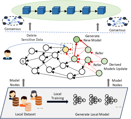
Figure 1. This figure provides an overview of the proposed framework. The lower part of the figure illustrates the users involved in the FL task. These users refer to existing models in the FL model-sharing network for local model generation and create their own model as a node to be published in the network. The middle section describes the network for a user who wants to delete sensitive data (the yellow node). The user republishes the updated model (the green node), and subsequent models affected by it (the green lattice nodes) also be updated. The upper part of the figure shows that both the publication and the update of the model are recorded in the blockchain.

Candidate models. A participant uses its local test dataset $D^{test}$ to randomly select a number of models contributed by other users for evaluation. Subsequently, the participant obtains the test accuracy set $AC^{test}$ of these models until collecting $K$ candidate model set $W^{\ast}$, as given by

(1) $$\begin{split}(AC^{test},W^{\ast})&=\left\{(F(w_{i},D^{test}),w_{i})\,\middle|\,w_{i}\in K,\right.\\ &\left.\,i=1,2,\cdots,k\right\},\end{split}$$

where $F\left(\cdot\right)$ denotes that the participant evaluates the model on its own test dataset $D^{test}$ using the model $w_{i}$ and obtains an accuracy. Then, this function returns the accuracy value.

Selection and aggregation. The participant selects the top $\mathbb{N}$ models in terms of accuracy ranking from the previous randomly selected $K$. Then, the participant uses model aggregation to obtain a pre-aggregation model $\tilde{W}$, as given by

(2) $$\tilde{W}=\sum_{w_{n}\in W}\frac{1}{N^{R_{n}}}w_{n},$$

where $W$ is the set of models in the top $\mathbb{N}$ ranks and $N^{R_{n}}$ is the number of referenced models associated with model $w_{n}$.

Training. The participant trains $\tilde{W}$ with its local training dataset $D^{train}$ to obtain the final aggregated model $W$:

(3) $$W=\daleth\left(\tilde{W},\phi,D^{train}\right),$$

where $\phi$ denotes the training settings, including the learning rate and batch size; and $\daleth\left(\cdot\right)$ denotes the participant’s training function for the task.

Evaluation. After training completion, the participant evaluates the model on its local test dataset $D^{test}$ to obtain the final accuracy $AC$.

Generate node. The participant prepares a model node $mv_{j}$ that includes the accuracy set $\mathbb{A}\mathbb{C}$ and model set $\mathbb{W}$ from the referenced $\mathbb{N}$ models, the CH value $CH(W)$ of the model, the identifier $URI(W)$ of the model, $AC$, $\phi$ and the creation timestamp $T_{mv_{j}}$. Then, the participant signs the $mv_{j}$, and broadcasts the signed nodes in the network.

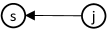
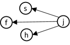
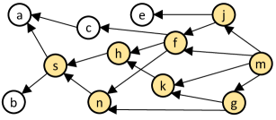
Figure 2. (a) Shows a one-to-one reference relation. (b) Model $w_{j}$ references three models, $w_{s}$, $w_{f}$ and $w_{h}$, so $R_{j}=\left\{r_{j\rightarrow s},r_{j\rightarrow f},r_{j\rightarrow h}\right\}$. (c) Between $w_{s}$ and $w_{m}$, the models affected by model $w_{s}$ are $w_{n}$, $w_{h}$, $w_{k}$, $w_{f}$, $w_{j}$ and $w_{g}$. Therefore, the set of reference relations $\mathbb{R}_{m\rightarrow\cdots\rightarrow s}=\left\{R_{m},R_{g},R_{j},R_{f},R_{k},R_{h},R_{n}\right\}$.

3.3. Blockchain Structure Design

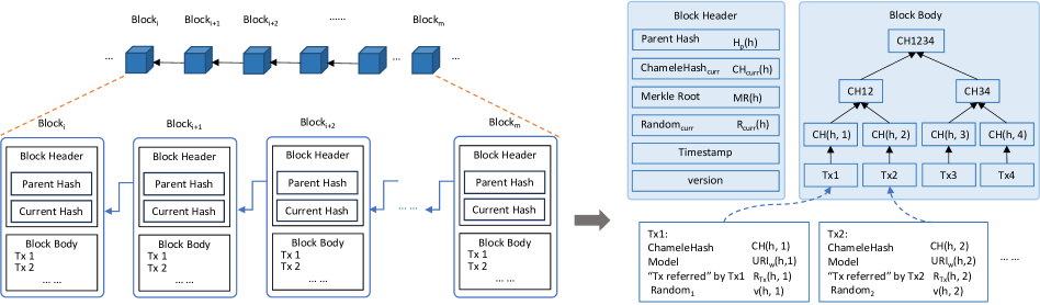
Figure 3. Blockchain structure. We link our blocks by having the hash of the current block’s parent point to the hash of the previous block. In the FL network, a node represents a model, and the model’s URI is embedded in a single transaction. Multiple transactions are included in a block. Updates in the blockchain manifest in two ways: (a) In the block body, the model URI and random number are updated, while other fields remain unchanged. As our transaction hash uses the CH value, the update does not affect the value of the Merkle Root in the block header. (b) In the block header, each update task leads to updates in the version and random number, thus using the hash value of the current block as the CH value. This ensures that the linkage between blocks is not affected.

We have designed the structure of the blockchain, linking our blocks by having the hash of the current block’s parent point to the hash of the previous block. Each block consists of a block header and a block body, consistent with the structure of traditional blocks. In our blockchain structure, we use CH to ensure that transactions and block headers are redactable. This design enables BlockFUL to update multiple transactions and blocks simultaneously through a single committee consensus operation.

Block header. As shown in Fig. 3 for a block with height $H$. The block header contains the following six key fields.

- $H_{p}\left(h\right)$: This is the parent hash of the block before linking.

- $CH_{curr}\left(h\right)$: Considering a model update task, it functions as the hash value for the current block. This role ensures that changes in the model version resulting from updates do not affect the validity of the current block.

- $R_{curr}\left(h\right)$: The latest random number for version-based CH value.

- $version$: This field is updated with the corresponding version number for each update task, maintaining consistent versions in the global state.

There is also the common block body’s Merkle root $MR(h)$ and the current block generation time $timestamp$.

Block body. A block body contains multiple redactable transactions uniformly composed in a Merkle tree structure and stores model-related values. A redactable transaction contains the following fields. Here, we take transaction $Tx_{i,j}$ as an example, i.e., the $j$-th transaction in the body of block $i$.

- CH Value $CH\left(i,j\right)$: This is the CH value of a transaction, and the field remains unchanged because it is involved in the $MR(h)$ calculation.

- Random Number $v(i,j)$: This field stores the latest random number used to compute the CH value based on $URI_{w}\left(i,j\right)$.

- Model $URI_{w}\left(i,j\right)$: This field stores the identifier of the model linked to the transaction. Only one model identifier is recorded per transaction. According to $URI_{w}\left(i,j\right)$, we can find the corresponding model in IPFS.

- $Tx_{i,j}$ referred list $R_{Tx}\left(i,j\right)$: It stores the relations with up to $N$ transactions with models being referred by the model in $Tx_{i,j}$. Based on all the reference transaction lists in the blockchain, we can obtain the reference relations of all models in the BlockFUL task.

The design of this block contributes to achieving efficient and secure redactability in the blockchain. On the one hand, due to the use of CH, transaction updates do not alter the block body’s Merkle root. However, the version field in the block header may cause collaborative updating issues with the block header. To ensure the consistency of transaction versions, we introduce the $version$ field. As a result, the validity of the link between blocks is maintained, and computational overhead is minimized. Moreover, $CH\left(i,j\right)$ is a field in the block that needs verification for the block body. In this way, even if $URI_{w}\left(i,j\right)$ and $v(i,j)$ are updated, $CH(i,j)$ in the block body remains unchanged. Thus, $MR(h)$ in the block header also remains unchanged. These conditions satisfy the immutability of $CH_{curr}\left(h\right)$ and $CH(i,j)$, respectively.

A valid block with an immutable block header can still be verified. On the other hand, this redactability does not compromise the tamper-resistance of the blockchain. The redactability of blocks is guaranteed by $CH_{sk}$ (trapdoor), an indispensable input for CH updates (Yu et al., 2020). Meanwhile, to prevent malicious committee members from deliberately exposing outdated transaction information, once a transaction becomes outdated, it will not be stored, but directly discarded. Similarly, outdated models in IPFS will also be directly discarded.

3.4. Unlearning Process

The unlearning process in BlockFUL consists of the inheritance unlearning phase and the blockchain unlearning phase.

Inheritance unlearning phase. The unlearning request is initiated by a specific node. All inherited models influenced by this node need to be updated, as shown by the green lattice nodes in Fig. 1. The updating process continues until the model nodes reach the latest generated nodes. The proposed unlearning framework supports various inheritance unlearning methods. Two cases are given in Section 4.

Blockchain unlearning phase. In subsection 3.3, we designed the blockchain structure. Each transaction has a $Tx$ reference list field to record the reference relations of its transactions. Based on these reference relations, we can obtain the reference relations of all transactions in the model inheritance training, i.e., the entire inheritance model network structure. Therefore, in the blockchain, we are able to update all inherited transactions comprehensively.

As mentioned earlier, during the initialization phase, the CH public-private key pair is generated by the users participating in FL. We first generate a private (trapdoor) key $CH_{sk}$ and a public (hash) key $CH_{pk}$ based on a security parameter $\lambda$ and a system parameter $CH_{para}$. The $CH_{pk}$ is broadcast to the network, and committee members in the blockchain each hold a $CH_{sk}$. Next, The computation involves hashing the model $URI_{w}(i,j)$, CH public key $CH_{pk}$, and a random number to generate the CH value. The calculation is as follows:

(4) $$CH\ Hash\left(URI_{w}(i,j),CH_{pk},v(i,j)\right)\rightarrow ChameleHash.$$

Updating the parameters equation related to $CH$, as shown in Eq. (5), ensures that the original $CH$ value remains valid after information updates. The committee inputs the model $URI_{w}(i,j)$ before the update, the model $URI^{\prime}_{w}(i,j)$ after the update, the random number $v(i,j)$ before the update, and the corresponding private key $CH_{sk}$. It outputs the updated random number $v^{\prime}(i,j)$, as follows:

(5) $$CH\ update\left(URI_{w}(i,j),URI^{\prime}_{w}(i,j),v(i,j),CH_{sk}\right)\rightarrow v^{\prime}(i,j).$$

Finally, by replacing the updated $URI^{\prime}_{w}(i,j)$ and $v^{\prime}(i,j)$ in the original $ChameleHash$, the output satisfies the following conditions:

(6) $$\begin{split}&CH\ hash\left(URI^{\prime}_{w}(i,j),CH_{pk},v^{\prime}(i,j)\right)=\\ &CH\ hash\left(URI_{w}(i,j),CH_{pk},v(i,j)\right).\end{split}$$

In addition, after the transaction update is completed, the block header needs to be updated. This is primarily done to update the version. Updating the version in the block header is consistent with the above process. Once the committee’s consensus nodes complete the transaction and block updates, they send them to other consensus nodes to complete the entire consensus process.

4. Block Federated Unlearning Schemes

In this section, we elaborate on the BlockFUL unlearning schemes, specifically focusing on updating model inheritance through the gradient ascent method and the re-training method. For both methods, we present the procedure and algorithm for unlearning the inherited model in BlockFUL and their computational cost. Note that the new approach using gradient ascent in our proposed BlockFUL unlearning framework also applies to distributed learning. When model nodes receive new data, they need to learn and can further update the models inherited from them.

4.1. Design Goal

Our goals for updating multiple models in parallel include accuracy in unlearning sensitive and non-sensitive data, effectively unlearning multiple categories of sensitive data, and reducing computational overhead.

G1. Comparable unlearning accuracy. In implementing unlearning, our goal is to ensure that the accuracy of the sensitive dataset approaches zero as closely as possible to minimize the risk of sensitive information leakage.

G2. Comparable non-unlearning accuracy. In implementing unlearning, this may lead to a slight decrease in accuracy for the non-sensitive dataset, even though the methods adopted may not be explicitly designed to improve accuracy. However, we still strive to ensure that there is only minimal difference in accuracy compared to the original model across unlearning tasks of different scales.

G3. Parallel multi-class unlearning. Users can upload multiple models to participate in the same FL task. When it’s necessary to delete sensitive data and update these models, parallel unlearning operations can be performed. These models may involve different categories of sensitive data, and the derived models of these models can be effectively updated.

G4. Reducing time overheads. Regardless of how many models are “forgotten” in the inheritance network, the gradient ascent method we employ should result in smaller computational costs compared to the re-training method.

4.2. Player Model

User. We make two assumptions about user behaviors. First, model references are time-sensitive, and new users joining the FL task cannot train with models from before a certain block height. Second, all users participating in the FL task are assumed to be honest and strictly adhere to the network task. Participating users do not infer models, and they do not re-train any version of the model before the unlearn operation. This assumption is fundamental to maintaining the integrity and confidentiality of the model.

Adversary. The attacker does not know the model before the unlearn operation, only the model after the unlearn operation. Having knowledge of the model before the unlearn operation does not hold significant value for an attacker. The primary focus is on safeguarding the model in its current state after the unlearning operation. This current state represents the real value and utility of the model, both from the user’s perspective and that of a potential attacker.

4.3. Scheme 1 - Gradient Ascent

Single start model. A user requesting to delete sensitive data re-trains the original model $w_{s}$ on its client to generate an updated model $w^{\prime}_{s}$. By calculating the difference between the gradients of the model before and after unlearning sensitive data, we can obtain $\nabla\theta_{s}$. Starting from a updated model $w^{\prime}_{s}$, a derived model $w_{j}$ of the original model $w_{s}$ is updated accordingly as

(7) $$w^{\prime}_{j}=\sum_{p_{l}\in P}\frac{1}{\prod_{R_{j}\in\mathbb{R}_{j\rightarrow\cdots\rightarrow s}}N^{R_{j}}}\times\alpha\nabla\theta_{s}+w_{j},$$

where $P$ denotes the set of paths from $w_{s}$ to $w_{j}$, $P=\left\{p_{1},\ldots,p_{l}\right\}$, $N^{R_{j}}$ denotes the number of models referenced by each model node passing through path $p_{l}$, and $\alpha$ denotes discount factor. This equation is formulated to handle model inheritance in FL, enabling the update of all relevant derived models. It offers insight into how model updates propagate through the inheritance structure, ensuring that modifications in the original model cascade appropriately to its derived counterparts.

Multiple start model. A user participating in a BlockFUL task contributes multiple models. During updates, these models serve as the starting update models and mutually influence each other. For a model $w_{j}$ affected by multiple starting model updates, the update results as

(8) $$w^{\prime}_{j}=\sum_{\begin{gathered}\nabla\theta_{s}\in\nabla\theta\\ P^{\nabla\theta_{s}}\in\mathbb{P}\end{gathered}}\left(\sum_{p^{\nabla\theta_{s}}_{l}\in P^{\nabla\theta_{s}}}\frac{1}{\prod_{R_{j}\in\mathbb{R}_{j\rightarrow\cdots\rightarrow s}}N^{R_{j}}}\times\alpha\nabla\theta_{s}\right)+w_{j},$$

where $\nabla\theta$ denotes the set of multiple model gradients for a user, $\nabla\theta=\left\{\nabla\theta_{1},\nabla\theta_{2},\ldots,\nabla\theta_{s}\right\}$, $p^{\nabla\theta_{s}}_{l}$ denotes the $l$-th path with gradient $\nabla\theta_{s}$ and $P^{\nabla\theta_{s}}$ denotes the set of paths with gradient $\nabla\theta_{s}$. Additionally, $\mathbb{P}$ denotes the set of paths with all gradients, $\mathbb{P}=\left\{P^{\nabla\theta_{1}},P^{\nabla\theta_{2}},\ldots,P^{\nabla\theta_{s}}\right\}$.

As shown in Eq. (7), derived model $w_{j}$ is influenced by updated model $w^{\prime}_{s}$. It is trained by referencing at least two models. Each model is referenced $N^{R_{j}}\geq 2$ times. This does not consider the special case where only one existing model is referenced. Since the key to derived model updates is related to $N^{R_{j}}$ and $\nabla\theta_{s}$, we cannot determine how much depth other models derived from $w^{\prime}_{s}$ need to go through before subsequent updates are no longer needed. Therefore, we introduce a predefined threshold $\varepsilon$ to indicate the depth of model convergence. It determines the minimum confidence level at which derived models stop updating. In addition, we use $\nabla\theta$ to denote the upward gradient and $d$ to denote the depth. For a given derived model, $P$ denotes the set of paths from $w_{s}$ to it , $P=\left\{p_{1},p_{2},\ldots,p_{l}\right\}$ , and $D$ denotes the set of depths corresponding to each path, $D=\left\{d_{1},d_{2},\ldots,d_{i}\right\}$.

Theorem 4.1.

The depth of model convergence for the number of model references $N^{R_{j}}\geq 2$ satisfies

(9) $$d_{i}>\log_{2}(\frac{|\nabla\theta|}{\varepsilon});$$

(10) $$\sum_{d_{i}\in D}\frac{1}{2^{d_{i}}}<\frac{\varepsilon}{|\nabla\theta|}.$$

Proof.

The proof can be found in Appendix A.1

∎

As can be seen from Theorem 4.1, the maximum depth of model convergence is determined by the variable $\nabla\theta$. Since $\nabla\theta$ is finite, there must exist some depth $d$ such that $d_{max}=\lceil log_{2}\frac{|\nabla\theta|}{\varepsilon}\rceil$. When $\nabla\theta$ is smaller, the model can converge faster. On the contrary, if $|\nabla\theta|$ is larger, the model converges slower. According to our previous description, in Eq. (7), the update of derived model is related to $N^{R_{j}}$ and $\nabla\theta_{s}$. Therefore, when $\nabla\theta_{s}$ is kept constant, the larger $N^{R_{j}}$ is, the faster the model converges, and vice versa, the slower it converges. In this case, the depth $d<d_{max}$.

If the model references a path in which only one model is referenced, then the depth of model convergence is $d+c$. Here, $c$ represents the number of nodes referencing only one model.

Corollary 4.2.

When multiple models of a user are used as starting points for updates, and there are interactions between these derived models. Derived models influenced by these models also reach a state of convergence at some depth.

Proof.

The proof can be found in Appendix A.2 ∎

Unlearning in BlockFUL. In Algo. 1, users broadcast the updated model message to the network. Upon receiving the message, the committee processes the starting updated model set $W$ and its inherited model set $N(W)$. According to Eq. (8), the committee performs gradient ascent updates on the inherited models. Similarly, these updates need to be executed on the blockchain. Since the reference transaction list $R_{Tx}$ in each transaction provides referencing relations for all transactions in the BlockFUL task. With the assistance of $CH_{sk}$, each committee member overwrites all transactions and versions to be updated in the blockchain. Based on all these updates, a hash value is uniformly calculated. This hash value is used to execute the consensus process, which helps prevent malicious committee members from making false updates.

1

2Define Receiver $\leftarrow$ Sender.Send(Message);

3// This transmission is secured by any private and encrypted channels, e.g., TLS.

4 Input: $G=(V,E)$, start model set $W^{\prime}$, start model $w^{\prime}_{i}\in W^{\prime}$, model gradient set $\nabla\theta$, learning rate $\alpha$

5for $w^{\prime}_{i}$ to $W^{\prime}$ parallel do

6       Send model_update message($w^{\prime}_{i}$);

7      // broadcast to the network.

8       for $w_{k}$ to $N(W)$ do

9             $w^{\prime}_{k}$ $\leftarrow$ Committee.Update($w_{k}$, $\nabla\theta$, $\alpha$);

10            // Update the model weights influenced with $W^{\prime}$ by Eq. (8).

11             $r^{\prime}_{i}$ $\leftarrow$ Committee.Overwrite$(URI(w_{i})$,

12            $URI(w^{\prime}_{i})$, $r_{i},CH_{sk}$);

13             $r^{\prime}_{version}\leftarrow Committee.Overwrite(version$,

14            $new$ $version$, $r_{version},CH_{sk}$);

15            

16       end for

17      

18 end for

19

20while Consensus do

21       Committee.Verify$(Hash(W^{\prime},N(W^{\prime}),r^{\prime},r^{\prime}_{version}))$;

22       if $Hash(W^{\prime},N(W^{\prime}),r^{\prime},r^{\prime}_{version})$ $is$ $invalid$ then

23             alarm and exit updated blocks;

24             Update the corresponding parameters in IPFS;

25            

26       end if

27      

28 end while

Algorithm 1 Gradient ascent model update

4.4. Scheme 2 - Re-training

Here, the same user model settings are used as in our gradient ascent method. The re-training method starts from the updated model $w^{\prime}_{s}$ and goes through all the paths to the model $w_{j}$.

Re-aggregation. According to pre-aggregation in Eq. (2), the re-aggregation model is expressed as

(11) $$\tilde{w}^{\prime}_{j}=\frac{1}{N^{R_{j}}}W^{\prime}_{j},$$

where $W^{\prime}_{j}$ denotes the updated set of the original selected model weights.

Re-training. According to training in Eq. (3), the users associated with these paths re-train the model on their own local clients. The derived model $w_{j}$ will be updated accordingly as

(12) $$w^{\prime}_{j}=\daleth_{j}\left(\tilde{w}^{\prime}_{j},\phi_{j},D^{train}_{j}\right).$$

Unlearning in BlockFUL. The method of model updating using re-training is shown in Algo. 2. In this process, the client first checks whether it is the starting update model. Otherwise, the client performs the operations of re-aggregation and re-training of its own model locally. Then, the client broadcasts the model update message to the network. Similarly, the committee utilizes $CH_{sk}$ in the blockchain to perform the same updating operations as in Algo. 1. Subsequently, consensus verification is conducted. Upon reaching a consensus, the committee updates the blocks and parameters accordingly in IPFS. Finally, the committee sends model update messages to the next-hop clients for model updating.

1

2Define All functions inherited from Algo. 1;

3 Input: $G=(V,E)$, start model set $W^{\prime}$, start model $w^{\prime}_{i}\in W$

4

5for $w^{\prime}_{i}$ to $W^{\prime}$ do

6       for $w_{k}$ to $N(W)$ do

7             if  $w_{k}$ $\neq$ $w^{\prime}_{i}$  then

8                   Re-aggregation according to Eq. (11); Re-training according to Eq. (12);

9             end if

10            Send model_update message($w^{\prime}_{i}$); // broadcast to the network. $r^{\prime}_{i}\leftarrow Committee.Overwrite(URI(w_{i})$,

11            $URI(w^{\prime}_{i})$, $r_{i},CH_{sk}$); $r^{\prime}_{version}\leftarrow Committee.Overwrite(version$,

12            $new$ $version$, $r_{version},CH_{sk}$);

13            while Consensus do

14                   Committee.Verify($W^{\prime},r^{\prime}_{i},r^{\prime}_{version}$);

15                   if $W^{\prime},r^{\prime}_{i},r^{\prime}_{version}$ $is$ $invalid$ then

16                         alarm and exit

17                         updated blocks;

18                         Update the corresponding parameters in IPFS;

19                        

20                   end if

21                  

22             end while

23            

24            Clients($N^{1}\left(W\right)$) $\leftarrow$ model_update message($W^{\prime}$); // Parallel transmission.

25       end for

26      

27 end for

Algorithm 2 Re-training model update

4.5. Cost Analysis

This subsection primarily analyzes the computational cost overheads of gradient ascent, re-training and block update. Here, the transmission cost $C_{tran}$ represents the cost associated with a single operation of uploading $C^{up}_{tran}$ or downloading $C^{down}_{tran}$ a model.The committee consensus cost is $C_{con}$. The cost of a single CH update operation is denoted by $C_{CH}$. Suppose $N$ blocks and $K$ models need to be updated, including $M$ starting models and $K-M$ inherited models.

Table 1. Comparison between The Gradient Acsent and Re-training Methods

Method	Computation Consumption	Update Role	Execution
Gradient Ascent	$(K-M+1)C_{GA}+(K+N)C_{CH}+C_{con}+2KC_{tran}$	Committee	Parallel
Re-training	$(K-M+1)C_{retrain}+2KC_{CH}+{K}C_{con}+2KC_{tran}+N^{R}(K-1)C_{tran}$	Client	Serial

Starting GA cost. For the starting models of gradient ascent (GA), these models are executed locally by the client in parallel. The cost of GA for the model is denoted as $C_{GA}$, and the update cost for the starting models of GA is represented as

(13) $$C^{start}_{GA}=C_{GA}.$$

Inheritance GA cost. The gradient ascent process of inherited models is executed by the committee. The update cost of GA for the inherited models is represented as

(14) $$C^{inher}_{GA}=(K-M)C_{GA}.$$

CH GA cost. The cost of CH includes the cost of transactions CH $C^{Tx}_{CH}$ and the cost of blocks CH $C^{block}_{CH}$ in the blockchain. The CH cost of GA is represented as

(15) $$C^{GA}_{CH}=KC^{Tx}_{CH}+NC^{block}_{CH}=(K+N)C_{CH}.$$

Block consensus GA cost. The committee executes the entire gradient ascent process, enabling consensus to be reached for multiple transactions or blocks simultaneously. The consensus cost of GA is represented as

(16) $$C^{GA}_{con}=C_{con}.$$

Transmission GA cost. The transmission cost of the model is primarily incurred by consensus nodes for uploading and downloading. Since consensus nodes can perform uploading and downloading tasks in parallel, the transmission cost of the model is represented as

(17) $$C^{GA}_{tran}=KC^{up}_{tran}+KC^{down}_{tran}=2KC_{tran}.$$

Starting re-training cost. For the starting models of re-training, these models are executed locally by the client in parallel. The cost of re-training for the model is denoted as $C_{retrain}$ and the update cost for the starting models of re-training is represented as

(18) $$C^{start}_{retrain}=C_{retrain}.$$

Inheritance re-training cost. The re-training process of inherited models is executed locally by these models’ clients. The re-training cost of inherited models is represented as

(19) $$C^{inher}_{retrain}=(K-M)C_{retrain}.$$

CH re-training cost. In this process, each transaction update requires one transaction CH and one block CH. The CH cost of re-training is represented as

(20) $$C^{retrain}_{CH}=KC^{Tx}_{CH}+KC^{block}_{CH}=2KC_{CH}.$$

Block consensus re-training cost. Each model update requires one round of consensus. The consensus cost for re-training is represented as

(21) $$C^{retrain}_{con}=KC_{con}.$$

Transmission re-training cost. The transmission cost of the model primarily involves the uploading and downloading processes by local clients, as well as the downloading process by consensus nodes. Suppose the average number of references per model is $N^{R}$. The transmission cost for re-training is represented as

(22) $$\begin{split}C^{retrain}_{tran}&=KC^{up}_{tran}+N^{R}(K-1)C^{down}_{tran}+KC^{down}_{tran}\\ &=2KC_{tran}+N^{R}(K-1)C_{tran}.\end{split}$$

The computational overhead of the two methods is compared in Table 1. We compared the computational costs, role updates, and update modes of the two methods. The re-training incurs higher expenses compared to gradient ascent, primarily due to consensus and transmission overheads.

For the case of one transaction corresponding to one block and the case of multiple transactions corresponding to one block, the block update costs can be represented as $SC_{block}$ and $MC_{block}$.

$Tx$-block. One or more transaction updates mainly go through CH overhead $C_{CH}$. Similarly, the main overhead is the same as the transaction overhead for one block or multiple block updates. Suppose that there are $K$ model updates. The costs can be given by

(23) $$SC_{block}=K(C^{block}_{CH}+C^{Tx}_{CH})=2KC_{CH}.$$

$Txs$-block. For the case of multiple transactions corresponding to a single block. Suppose there are $K$ model updates. The update cost in this block is

(24) $$MC_{block}=C^{block}_{CH}+KC^{Tx}_{CH}=(K+1)C_{CH}.$$

5. Experiments

In our experimental phase, we establish a simulation platform and assess the effectiveness of diverse obfuscation methods on sensitive data. We comprehensively evaluate the impact of these methods on accuracy for both sensitive and unrelated labels, incorporating classic models such as ResNet18 and MobileNetV2. We also evaluate the overhead of blockchain. This thorough analysis extends to measuring the time consumption during training and inference, providing insights into the trade-offs between privacy preservation and model performance within the BlockFUL framework.

5.1. Evaluation Metrics

Accuracy on sensitive dataset ($AD_{f}$). The accuracy of sensitive dataset of unlearning model. It should be close to zero.

Accuracy on non-sensitive dataset ($AD_{r}$). The accuracy of non-sensitive dataset of unlearning model. It should be close to the performance of the original model.

Unlearning class prediction distribution. We analyze the distribution of different samples of predictions in the unlearning model across sensitive data categories. If the number of different samples of predictions in sensitive categories is low, it indicates that the unlearned model is robust.

Unlearning time. The duration it takes for a model to unlearning or discard previously acquired information during the training process in machine learning and deep learning. The faster, the better.

Table 2. Unlearning Performance On CIFAR-10

Model	#$C_{f}$	Metrics	Original Model			Re-train Model			Gradient Ascent			Unlearning Time (ms)
												Re-training			Gradient Ascent
			$r_{1}$	$r_{2}$	$r_{3}$	$r_{1}$	$r_{2}$	$r_{3}$	$r_{1}$	$r_{2}$	$r_{3}$	$r_{1}$	$r_{2}$	$r_{3}$	$r_{1}$	$r_{2}$	$r_{3}$
MobileleNetV2	1	$A_{D_{r}}\uparrow$	81.36%	71.44%	99.40%	79.92%	82.85%	96.83%	51.53%	44.59%	42.02%	181.09	361.77	596.89	28.32	29.9	31.28
		$A_{D_{f}}\downarrow$	77.44%	77.04%	99.98%	0.00%	0.00%	0.00%	7.39%	8.52%	8.60%
	2	$A_{D_{r}}\uparrow$	98.56%	87.71%	82.49%	89.45%	78.76%	87.94%	53.64%	30.56%	17.56%	181.94	376.88	583.02	28.62	29.34	30.09
		$A_{D_{f}}\downarrow$	79.40%	86.21%	78.42%	0.00%	0.00%	0.00%	8.00%	7.16%	5.54%
	4	$A_{D_{r}}\uparrow$	92.43%	86.99%	86.70%	86.15%	94.37%	94.84%	50.97%	35.80%	16.58%	151.14	311.59	471.64	28.66	29.98	32.98
		$A_{D_{f}}\downarrow$	74.46%	74.11%	90.09%	0.00%	0.00%	0.00%	6.55%	9.36%	0.00%
	7	$A_{D_{r}}\uparrow$	92.30%	99.99%	97.39%	99.99%	99.99%	99.29%	51.87%	52.99%	36.53%	84.55	164.17	245.01	28.40	30.38	32.21
		$A_{D_{f}}\downarrow$	90.15%	91.86%	91.68%	0.00%	0.00%	0.00%	8.75%	4.32%	7.90%
ResNet18	1	$A_{D_{r}}\uparrow$	99.99%	99.99%	89.25%	99.99%	95.85%	99.99%	60.64%	52.78%	54.95%	312.95	625.27	951.14	28.62	30.05	31.59
		$A_{D_{f}}\downarrow$	99.99%	99.99%	92.73%	0.00%	0.00%	0.00%	7.76%	8.38%	6.78%
	2	$A_{D_{r}}\uparrow$	74.63%	90.09%	95.28%	99.99%	94.13%	91.95%	52.22%	60.17%	72.05%	290.76	597.86	907.71	28.67	29.8	31.03
		$A_{D_{f}}\downarrow$	98.82%	90.43%	97.70%	0.00%	0.00%	0.00%	8.95%	5.23%	3.45%
	4	$A_{D_{r}}\uparrow$	80.08%	88.00%	99.87%	90.42%	98.54%	99.95%	41.83%	58.00%	63.92%	218.85	442.17	664.46	28.55	29.86	30.83
		$A_{D_{f}}\downarrow$	89.21%	82.15%	99.68%	0.00%	0.00%	0.00%	4.50%	9.49%	8.50%
	7	$A_{D_{r}}\uparrow$	92.49%	90.19%	98.31%	99.95%	87.81%	99.99%	80.51%	54.49%	48.09%	134.04	264.57	391.35	28.54	30.66	32.27
		$A_{D_{f}}\downarrow$	84.14%	81.98%	97.50%	0.00%	0.00%	0.00%	6.00%	8.52%	7.35%

Table 3. Unlearning Performance On Fashion-MNIST

Model	#$C_{f}$	Metrics	Original Model			Re-training Model			Gradient Ascent			Unlearning Time (ms)
												Re-training			Gradient Ascent
			$r_{1}$	$r_{2}$	$r_{3}$	$r_{1}$	$r_{2}$	$r_{3}$	$r_{1}$	$r_{2}$	$r_{3}$	$r_{1}$	$r_{2}$	$r_{3}$	$r_{1}$	$r_{2}$	$r_{3}$
AlexNet	1	$A_{D_{r}}\uparrow$	99.99%	99.99%	99.81%	99.99%	99.99%	98.80%	90.38%	84.36%	72.50%	43.57	84.85	126.45	27.72	27.98	28.15
		$A_{D_{f}}\downarrow$	99.99%	99.99%	99.66%	0.00%	0.00%	0.00%	4.00%	3.99%	0.00%
	2	$A_{D_{r}}\uparrow$	99.99%	99.99%	99.80%	99.99%	99.99%	99.51%	81.71%	62.08%	74.26%	42.25	82.33	122.15	27.71	28.07	28.33
		$A_{D_{f}}\downarrow$	99.99%	99.99%	99.49%	0.00%	0.00%	0.00%	0.00%	0.00%	5.00%
	4	$A_{D_{r}}\uparrow$	99.99%	99.99%	99.96%	99.99%	99.99%	99.16%	72.14%	66.52%	61.03%	40.34	77.65	115.51	27.71	28.51	28.91
		$A_{D_{f}}\downarrow$	99.99%	99.99%	99.89%	0.00%	0.00%	0.00%	7.00%	0.00%	0.00%
	7	$A_{D_{r}}\uparrow$	99.99%	99.99%	99.72%	99.71%	92.72%	90.84%	90.16%	92.82%	84.03%	35.09	69.72	103.77	28.4	29.75	30.89
		$A_{D_{f}}\downarrow$	99.99%	99.99%	98.82%	0.00%	0.00%	0.00%	0.00%	0.00%	0.00%
ResNet18	1	$A_{D_{r}}\uparrow$	99.90%	99.73%	94.10%	95.36%	83.35%	94.11%	82.35%	86.08%	84.69%	261.35	515.62	763.3	27.87	28.39	28.93
		$A_{D_{f}}\downarrow$	99.99%	99.99%	94.49%	0.00%	0.00%	0.00%	0.00%	3.85%	6.27%
	2	$A_{D_{r}}\uparrow$	92.74%	92.74%	99.64%	95.67%	97.44%	91.37%	29.30%	64.45%	41.28%	236.34	465.44	697.74	28.03	28.77	29.42
		$A_{D_{f}}\downarrow$	95.75%	95.70%	98.35%	0.00%	0.00%	0.00%	5.00%	5.22%	1.81%
	4	$A_{D_{r}}\uparrow$	95.77%	98.97%	98.48%	99.96%	98.43%	95.02%	45.46%	69.25%	51.18%	175.26	353.09	532.84	28.27	29.49	30.7
		$A_{D_{f}}\downarrow$	62.73%	95.02%	99.71%	0.00%	0.00%	0.00%	9.75%	2.63%	0.12%
	7	$A_{D_{r}}\uparrow$	91.48%	87.32%	85.49%	92.59%	89.85%	98.61%	50.06%	32.05%	32.05%	115.51	223.26	330.35	28.56	30.67	32.72
		$A_{D_{f}}\downarrow$	74.46%	89.32%	91.84%	0.00%	0.00%	0.00%	5.57%	0.00%	0.00%

5.2. Datasets

In this subsection, we provide a brief overview of the datasets utilized in the experiments, encompassing two types as outlined below:

CIFAR-10. CIFAR-10 is a widely used dataset for image classification tasks in computer vision. It consists of 60,000 32x32 color images in 10 different classes, with 6,000 images per class. The dataset is split into 50,000 training images and 10,000 testing images.
Fashion-MNIST. Fashion-MNIST is a commonly used dataset for image classification tasks, similar to MNIST but more challenging. The dataset comprises ten fashion categories, each comprising 60,000 grayscale images with dimensions of 28x28 pixels. The training set contains 55,000 images, while the test set includes 10,000 images.

5.3. Compared Methods

In our comparison study, we employ the following unlearning methods:

Re-training. We re-train the sensitive model with a dataset containing sensitive data and the derivative models influenced by it. We remove sensitive data from this dataset and sequentially train using the remaining data according to the reference relation.
Gradient ascent. This involves the reference relation where models are uploaded by users with sensitive data. For the initial sensitive models, we calculate the difference in the model gradient before and after unlearning. Subsequently, the referenced models utilize this gradient difference for gradient ascent. By assessing these gradients, we gain insights into the impact of re-training on the models downstream, allowing for a comprehensive understanding of the unlearning process.

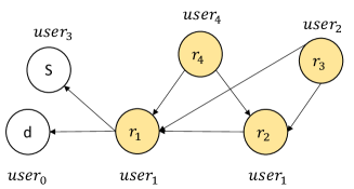
Figure 4. There are five users, and each arrow represents the aggregated model. The yellow color indicates sensitive data models and their inheritance models.

5.4. Experimental Settings

In the experimental setup, we conduct experiments using an NVIDIA GeForce RTX 3070 GPU. We employ an untrained ResNet18 model, a MobileNetV2 model, and an AlexNet model. All fine-tuned on specific datasets. The classes “forgotten” during the process are represented as #$C_{f}$.

For the reference relation framework, we involve a group of 5 users, as depicted in Fig. 4. $user_{1}$ and $user_{2}$ have labels of the same sensitive type, and the models highlighted in yellow are those that demonstrate accuracy on sensitive data.

Blockchain. In blockchain, we use PBFT consensus to ensure data consistency and security. Additionally, we have set the block packaging time to 15 seconds. This interval strikes a balance between transaction processing speed and network stability. Each block is sized at 1MB to ensure efficient network transmission and storage. CIFAR-10. In the CIFAR-10 setup, each model undergoes rigorous training for 100 epochs with a learning rate set to 0.005. The dataset encompasses distinct categories, each containing approximately 800 data samples. We strategically apply the unlearning process to both individual categories and various combinations, including 2, 4, 7, and so on. Here, $r_{1}$, $r_{2}$, and $r_{3}$ represent the models targeted for unlearning.
Fashion-MNIST. In the context of the Fashion-MNIST configuration, each model undergoes extensive training for 100 epochs with a learning rate set to 0.005. The dataset consists of distinct categories, each containing approximately 1000 data samples. The unlearning process is strategically applied to both individual categories and various combinations, including 1, 2, 4, 7, and so forth. The models designated for unlearning are referred to as $r_{1}$, $r_{2}$, and $r_{3}$.

5.5. Results

Our results compare the performance differences between the re-training method and the gradient ascent method. Furthermore, we analyze the outcomes of unlearning for individual classes and multiple classes.

CIFAR-10. We show the analysis results of $D_{r}$, $D_{f}$ and unlearning time in Table 2. Compared to the gradient ascent method, the re-train method performs the best in terms of accuracy for $D_{r}$ and $D_{f}$. In comparison to the re-train method, the gradient ascent method shows good unlearning effects for $D_{f}$, and the unlearning time can be maximally improved by 98.25% compared to re-training.
Fashion-MNIST. In the FASHION-MNIST dataset, we use AlexNet for predictions. It can be observed that the re-training time of AlexNet is much shorter compared to ResNet18. This suggests that in the case of models with fewer parameters, the re-training method can achieve better unlearning effects. Moreover, the unlearning effect of AlexNet is significantly better than ResNet18 in terms of $D_{r}$. It can be observed that the effectiveness of the gradient ascent method varies for different datasets and models.

Weight distance analysis. We conducted an analysis of the ResNet18 model using the Fashion-MNIST dataset. In the presence of sensitive data ($\#C_{f}=1$), we evaluated the distance trend of the unlearning method. Additionally, we computed the layer-wise distances between the re-trained model and the original model, as well as between the gradient ascent method and the original model. We selected the top 10 layer-wise examples to show whether the gradient ascent method has a similar distance trend to the re-trained model. As shown in Fig. 5, we can see that the gradient ascent model has a similar trend to the re-trained model, proving the effectiveness of the gradient ascent method.

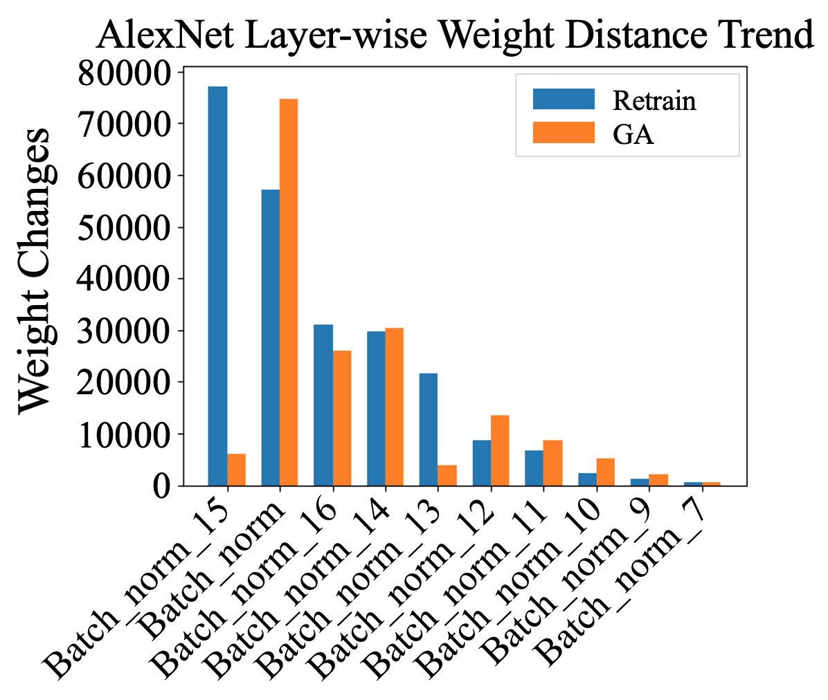
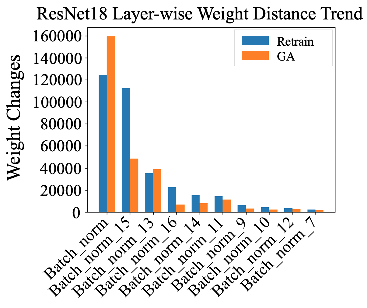
Figure 5. The sensitive data type is $\#C_{f}=1$. (a) and (b) depict the weight distances for ResNet18 on $r_{1}$ and $r_{3}$, respectively.

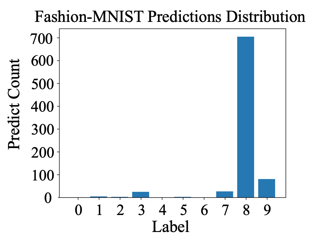
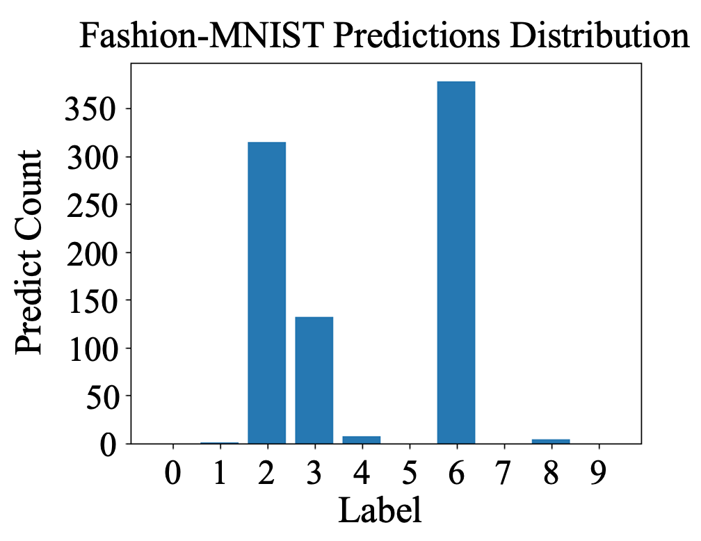
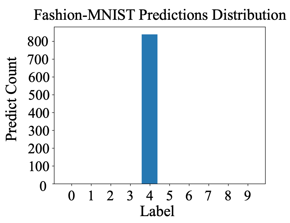
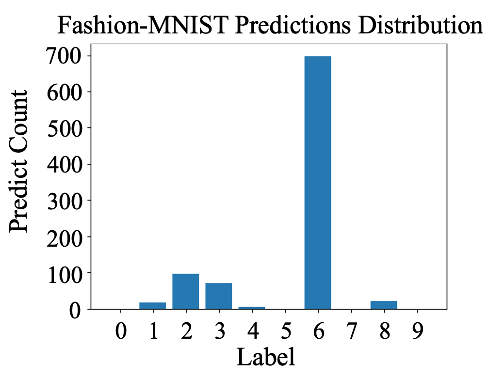
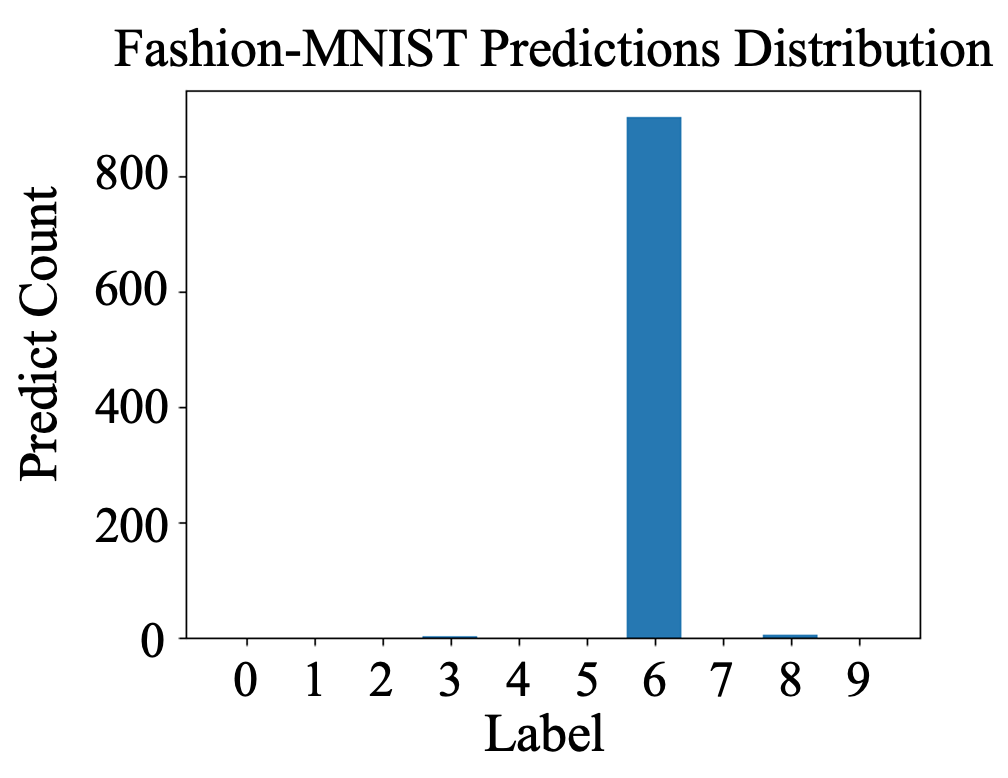
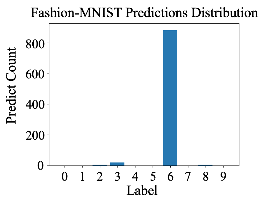
Figure 6. The sensitive data type is 0, (a) and (b) represent the re-trained ResNet18 on $r_{1}$ and $r_{2}$, respectively; and (c) and (d) represent the gradient ascent ResNet18 on $r_{1}$ and $r_{2}$, respectively; (e) and (f) represent the re-trained AlexNet on $r_{1}$ and $r_{2}$, respectively; and (g) and (h) represent the gradient ascent AlexNet on $r_{1}$ and $r_{2}$, respectively. The figure shows the prediction distribution of the unlearned model on the class of data to be “forgotten”. Our method gives a randomized response to the input query of the class of data to be “forgotten”.

5.6. Prediction Distribution

In Fashion-MNIST, we utilize the ResNet18 and AlexNet models to unlearn single-class sensitive data belonging to category 0 and multi-class sensitive data belonging to categories 0-6. After unlearning, we employ the unlearned model to predict sensitive data and analyze the distribution of predicted samples.

Single-class prediction. Figs. 6 and 6 illustrate the re-training unlearning of ResNet18 model for $r_{1}$ and $r_{2}$, while Figs. 6 and 6 depict the gradient ascent unlearning of ResNet18 model for $r_{1}$ and $r_{2}$. Similarly, Figs. 6 and 6 represent the re-train unlearning of AlexNet model for $r_{1}$ and $r_{2}$, respectively; Figs. 6 and 6 demonstrate the gradient ascent unlearning of AlexNet model for $r_{1}$ and $r_{2}$, respectively. We observe that both re-training and gradient ascent methods for ResNet18 model cannot predict the sensitive label 0. However, for the gradient ascent method of the AlexNet model, 6 can randomly predict the sensitive label 0, indicating a lack of robustness in the AlexNet model.

Multiple-class prediction. Figs. 7 and 7 are the re-training unlearning Resnet18 model for $r_{1}$ and $r_{2}$, respectively. Figs. 7 and 7 are the gradient ascent-based unlearning Resnet18 model for $r_{1}$ and $r_{2}$. Figs. 7 and 7 are the re-training unlearning AlexNet model for $r_{1}$ and $r_{2}$. Figs. 7 and 7 are the gradient ascent unlearning AlexNet model for $r_{1}$ and $r_{2}$. The sensitive data types range from category 0 to 6, from Figs. 7 and 7 we found through the gradient ascent method that the AlexNet model can still predict the sensitive label, but for the ResNet18 model Fig. 7 sensitive data 0 can still be randomly predicted, but other sensitive labels cannot be accurately predicted, demonstrating that ResNet18 exhibits a certain level of robustness across multiple sensitive labels.

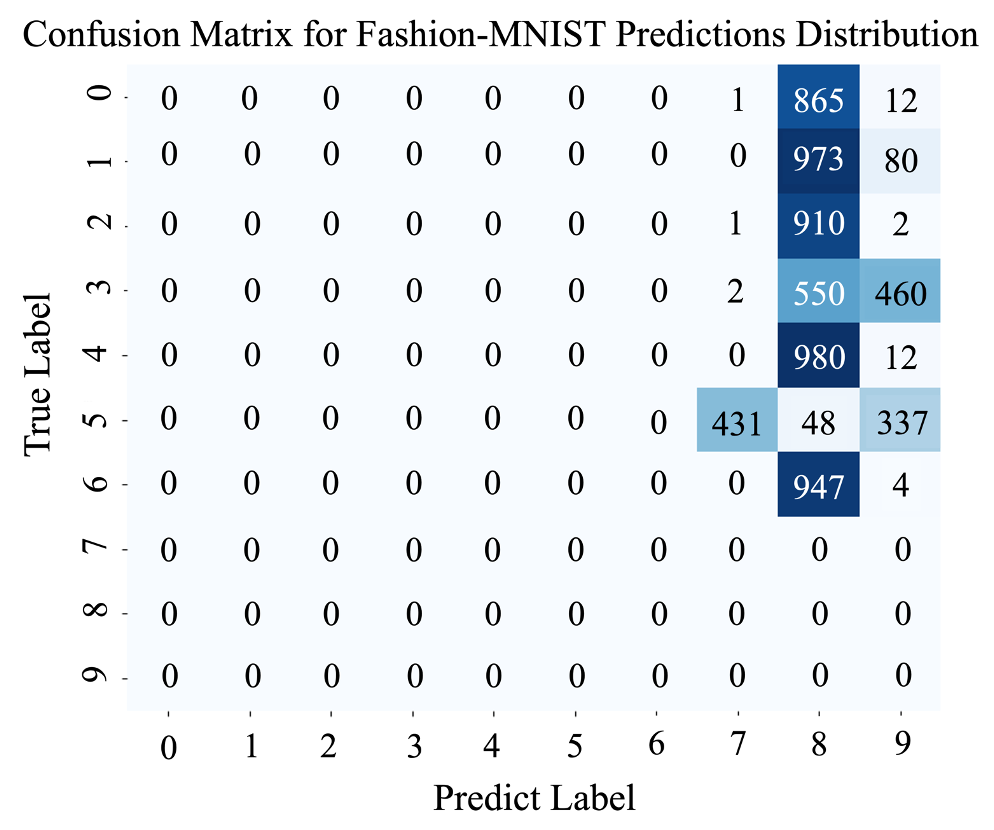
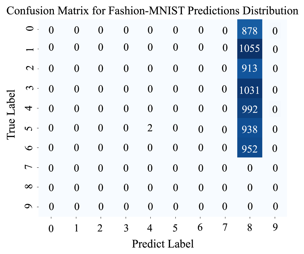
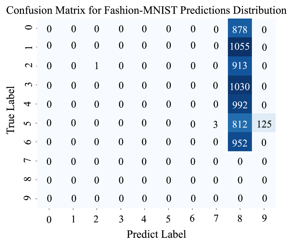
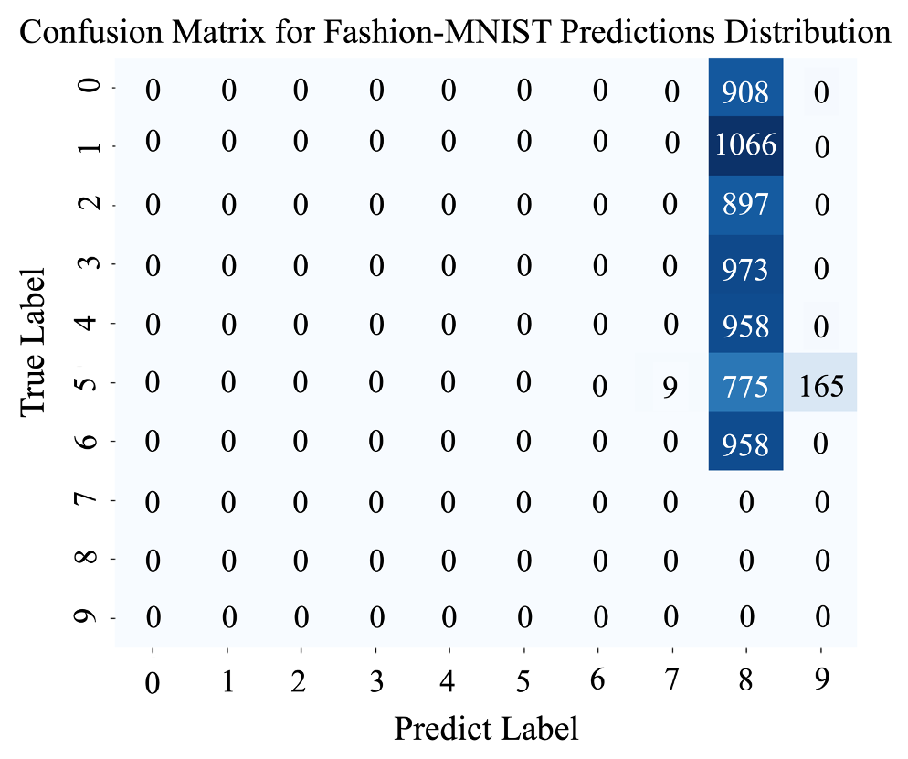
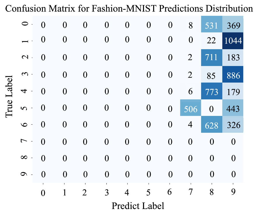
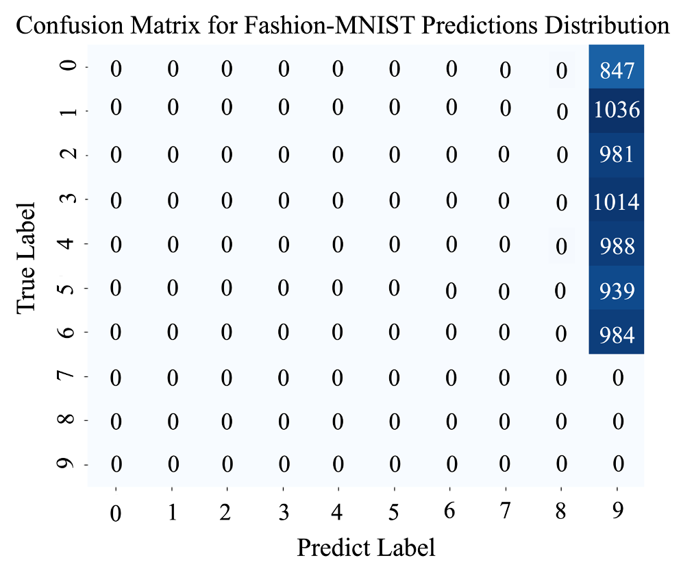
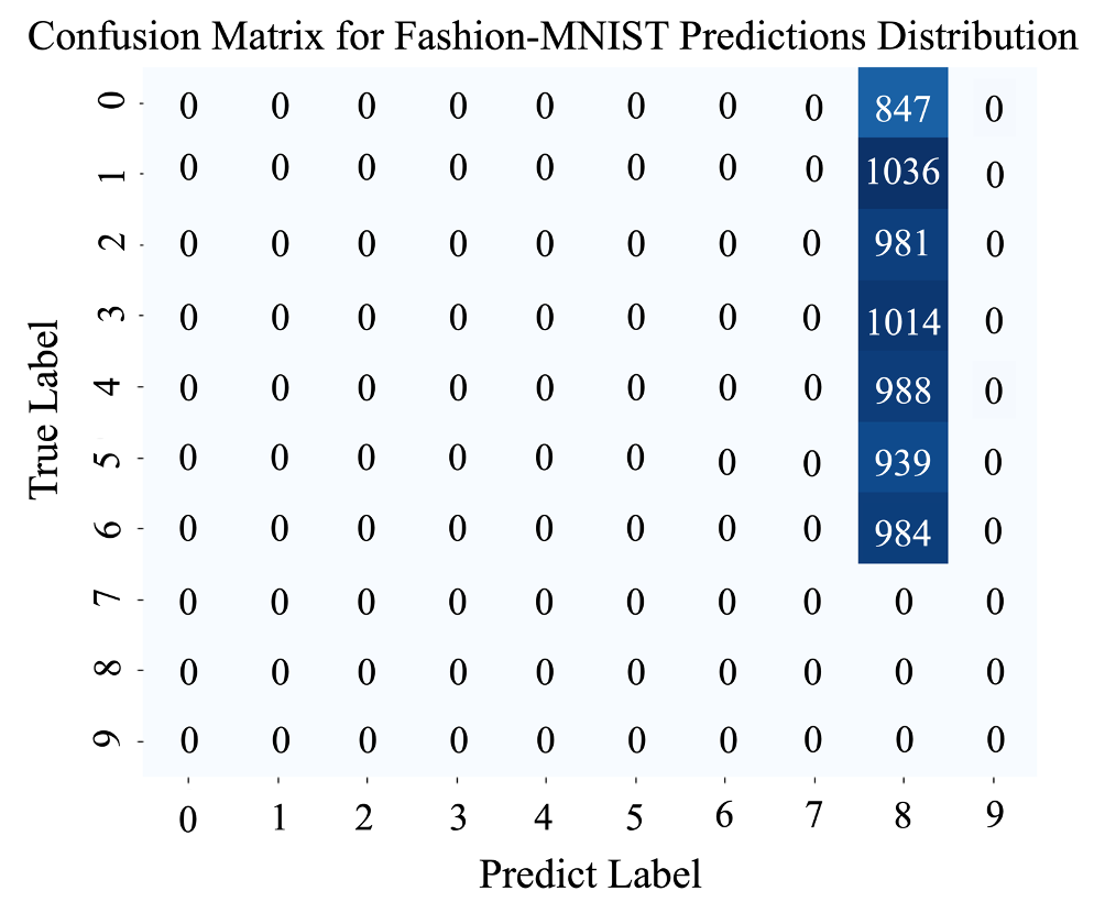
Figure 7. The sensitive data types range from category 0 to 6, (a) and (b) represent the re-trained AlexNet on $r_{1}$ and $r_{2}$, respectively and (c) and (d) represent the gradient ascent AlexNet on $r_{1}$ and $r_{2}$, respectively, (e) and (f) represent the re-trained ResNet18 on $r_{1}$ and $r_{2}$ respectively and (g) and (h) represent the gradient ascent ResNet18 on $r_{1}$ and $r_{2}$, respectively. The figures show the prediction distribution of the unlearned model on the class of data to be “forgotten”. Our method gives a randomized response to the input query of the class of data to be “forgotten”.

5.7. Cost Evaluation

In this section, we analyze the time overhead of blockchain execution under the re-training method and gradient ascent method. For each FL task, we establish a blockchain utilizing a single-chain structure. The network utilizes the PBFT consensus mechanism.

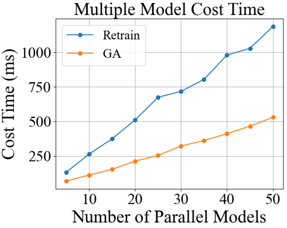
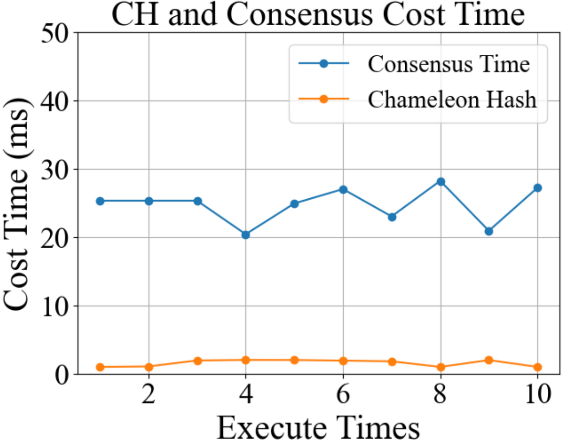
Figure 8. (a) represents the cost time of multiple start models; (b) represents the cost time of a single start model.

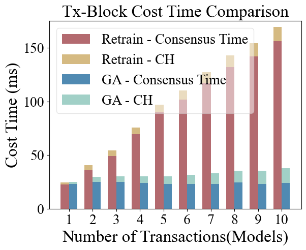
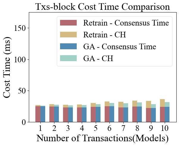
Figure 9. (a) represents the cost time of multiple blocks of inheritance models; (b) represents the cost time of a single block of inheritance model.

Multiple model parallel cost time. For both re-training and gradient ascent methods, we analyze the blockchain overhead incurred when multiple models are executed in parallel. We assume a DAG graph with only two models and the two models in different blocks, as illustrated in Fig. 8. It can be observed that both the re-training and gradient ascent methods demonstrate linear growth. This phenomenon arises from the inherent competition for network and computational resources within the PBFT consensus. The gradient ascent method incurs a maximum increase in time overhead of 124% compared to the re-training method.

Chameleon hash and consensus cost time. We conducted multiple trials to measure the chameleon hash and consensus computational overhead time for a single model, as illustrated in Fig. 8. The execution time of chameleon hash and consensus remains consistently within a constant range. Consensus time is 92% larger than chameleon hash time, occupying the majority of the blockchain overhead time.

$Tx$-block cost time. For the case where one transaction belongs to one block, we conducted experiments across multiple instances across different blocks, following Eq. (19). The horizontal axis represents the number of transactions (the number of unlearning models), and the vertical axis represents cost time. The experiments are illustrated in Fig. 9, where we observe a linear increase in time consumption as the number of inheritance models increases for both methods. Compared to re-training, gradient ascent achieves a maximum performance improvement of 75.8%.

$Txs$-block cost time. For the scenario where multiple transactions belong to a single block, we conducted experiments as depicted in Fig. 9, following Eq. (22), where the time consumption linearly increases with the number of inheritance models for both methods. However, compared to Fig. 9, the time consumption is lower than transactions across different blocks. For the re-training method and the gradient ascent method, the maximum improvements are 4.4% and 12.6%, respectively. This is due to the overhead incurred by multiple block updates. The gradient ascent method achieves a maximum improvement of 78.1% compared to re-training. This is attributed to the fact that gradient ascent only necessitates consensus once, whereas re-training imposes substantial overhead with every model update from the client, owing to the consensus requirement.

Chameleon hash overhead. We experiment with the computational overhead of chameleon hash on the blockchain. We use the structure in Fig. 4 to modify the hash values of the model $URI$ for the $r_{1}$ to $r_{4}$ nodes. One transaction corresponds to one block followed by Eq. (15), where $K=N=4$. As can be seen from Fig. 10, the modification time for each node is very short and within acceptable limits, the computational overhead grows linearly with the number of references, and the overhead of the two methods is approximately the same.

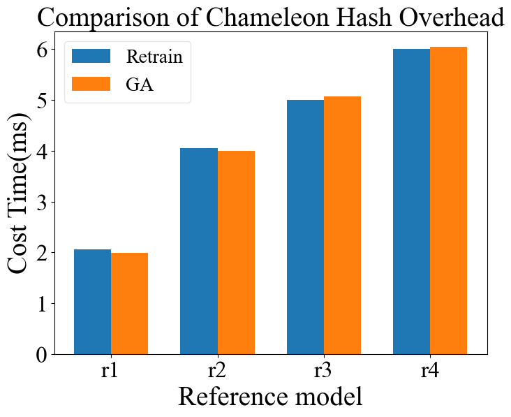
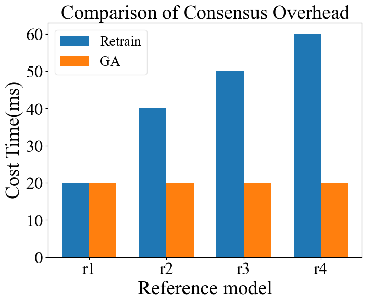
Figure 10. (a) represents chameleon hash cost time; (b) represents consensus cost time.

Blockchain consensus overhead. We conduct experiments employing the PBFT consensus on the DAG structure illustrated in Fig. 4, as detailed in Fig. 10. For the re-training method, our observations reveal that the time required also escalates as the reference number increases. However, for gradient ascent, we only need to conduct consensus once, so the overhead does not increase as the reference count grows. Notably, in comparison to the chameleon hash overhead, the consensus overhead dominates the majority. Thus, we have the flexibility to choose different consensus algorithms based on security and efficiency requirements.

6. Conclusion

For the Blockchained FL structure we considered with the characteristic of model inheritance, existing unlearning methods were either unavailable or increased the complexity of the unlearning operation. We posed two RQs: RQ1. How can Blockchained FL frameworks be enhanced to support unlearning tasks on any historical models while addressing the challenge posed by model inheritance in distributed FL systems? RQ2. Which unlearning schemes can be adapted for unlearning tasks in Blockchained FL? What are their performance and costs?

In response to these RQs, this paper proposed BlockFUL, a generic Blockchained FL framework, which supports various unlearning methods. The framework solves, for the first time, the problem of additional complexity and overhead caused by model inheritance unlearning. It enabled such “incremental” learning in a fully decentralized scenario and satisfied the need for multiple models to perform unlearning operations simultaneously. We conducted simulation experiments comparing the gradient ascent method with a baseline re-training method. The results show that the gradient ascent unlearning method is more economical in terms of time cost and superior in terms of model utility.

Appendix A Appendix

A.1. Proof of Theorem 4.1

First, in Eq. (7), we want to obtain

(25) $$|w^{\prime}_{j}-w_{j}|=\sum_{p_{l}\in P}\frac{1}{\prod_{R_{j}\in\mathbb{R}_{j\rightarrow\cdots\rightarrow s}}N^{R_{j}}}\times|\nabla\theta|<\varepsilon.$$

As discussed earlier, on a path $p_{l}$, $w_{s}$ passes through multiple model nodes to reach a model $w_{j}$ of depth $d$. The number of references per model is $N^{R_{j}}\geq 2$, with the corresponding $\frac{1}{N^{R_{j}}}\leq\frac{1}{2}$. For this path $p_{l}$, we have

(26) $$\frac{1}{\prod_{R_{j}\in\mathbb{R}_{j\rightarrow\cdots\rightarrow s}}N^{R_{j}}}\leqslant\frac{1}{2^{d}}.$$

Further, after passing through several model nodes, $w_{s}$ inevitably arrives at a model of depth $d$, to obtain

(27) $$\frac{|\nabla\theta|}{\prod_{R_{j}\in\mathbb{R}_{j\rightarrow\cdots\rightarrow s}}N^{R_{j}}}\leqslant\frac{|\nabla\theta|}{2^{d}}<\varepsilon.$$

For a $p_{l}$ path, we have

(28) $$2^{d}>\frac{|\nabla\theta|}{\varepsilon},\Longrightarrow d>log_{2}(\frac{|\nabla\theta|}{\varepsilon}).$$

For a set $P$ of all paths, we have

(29) $$\begin{split}&\sum_{p_{l}\in P}\frac{|\nabla\theta|}{\prod_{R_{j}\in\mathbb{R}_{j\rightarrow\cdots\rightarrow s}}N^{R_{j}}}\leqslant\sum_{d_{i}\in D}\frac{|\nabla\theta|}{2^{d_{i}}}<\varepsilon,\\ &\Longrightarrow\sum_{d_{i}\in D}\frac{1}{2^{d_{i}}}<\frac{\varepsilon}{|\nabla\theta|}\end{split}$$

If $\frac{1}{\prod_{R_{j}\in\mathbb{R}_{j\rightarrow\cdots\rightarrow s}}N^{R_{j}}}=\frac{1}{2^{d}}$ at this point, the value of $d$ can be obtained as

(30) $$d=\begin{cases}1,&\text{if }\log_{2}(\frac{|\nabla\theta|}{\varepsilon})<0;\\ \lceil\log_{2}\frac{|\nabla\theta|}{\varepsilon}\rceil,&\text{if }\log_{2}(\frac{|\nabla\theta|}{\varepsilon})\in\mathbb{R}^{+}\setminus\mathbb{Z}^{+}.\end{cases}$$

Theorem 1 is proved.

A.2. Proof of Corollary 4.2

According to Eq. (8), if we assume that the model $w_{j}$ is affected by multiple starting update models, we can use $B_{s}$ to represent the process of gradient ascent to $w_{j}$ for each different model. Here, $B_{s}=\sum_{p^{\nabla\theta_{s}}{l}\in P}\frac{1}{\prod\nolimits{R_{j}\in\mathbb{R}_{j\rightarrow\cdots\rightarrow s}}N^{R_{j}}}\times\nabla\theta_{s}$. Since multiple starting models are updated simultaneously, the gradient ascent process affected by the variable $\nabla\theta_{s}$ is actually the accumulation of individual gradient ascent values. In other words, $B=B_{1}+B_{2}+\cdots+B_{s}$. According to Theorem 4.1, a derived model influenced by the starting updated model eventually converges when a certain depth is reached. Therefore, as $\prod\nolimits_{R_{j}\in\mathbb{R}_{j\rightarrow\cdots\rightarrow s}}N^{R_{j}}$ increases, $B_{s}$ converge to $|w^{\prime}_{j}-w_{j}|<\varepsilon$, which further results in $B$ also converging to $|w^{\prime}_{j}-w_{j}|<\varepsilon$.

References

- (1)
- Bourtoule et al. (2021) Lucas Bourtoule, Varun Chandrasekaran, Christopher A Choquette-Choo, Hengrui Jia, Adelin Travers, Baiwu Zhang, David Lie, and Nicolas Papernot. 2021. Machine unlearning. In 2021 IEEE Symposium on Security and Privacy (SP). IEEE, 141–159.
- Cao and Yang (2015) Yinzhi Cao and Junfeng Yang. 2015. Towards making systems forget with machine unlearning. In 2015 IEEE symposium on security and privacy. IEEE, 463–480.
- Che et al. (2023) Tianshi Che, Yang Zhou, Zijie Zhang, Lingjuan Lyu, Ji Liu, Da Yan, Dejing Dou, and Jun Huan. 2023. Fast federated machine unlearning with nonlinear functional theory. In International conference on machine learning. PMLR, 4241–4268.
- Chen et al. (2022) Chong Chen, Fei Sun, Min Zhang, and Bolin Ding. 2022. Recommendation unlearning. In Proceedings of the ACM Web Conference 2022. 2768–2777.
- Chundawat et al. (2023) Vikram S Chundawat, Ayush K Tarun, Murari Mandal, and Mohan Kankanhalli. 2023. Zero-shot machine unlearning. IEEE Transactions on Information Forensics and Security (2023).
- Feng et al. (2021) Lei Feng, Yiqi Zhao, Shaoyong Guo, Xuesong Qiu, Wenjing Li, and Peng Yu. 2021. BAFL: A blockchain-based asynchronous federated learning framework. IEEE Trans. Comput. 71, 5 (2021), 1092–1103.
- Golatkar et al. (2020) Aditya Golatkar, Alessandro Achille, and Stefano Soatto. 2020. Eternal sunshine of the spotless net: Selective forgetting in deep networks. In Proceedings of the IEEE/CVF Conference on Computer Vision and Pattern Recognition. 9304–9312.
- Gupta et al. (2021) Varun Gupta, Christopher Jung, Seth Neel, Aaron Roth, Saeed Sharifi-Malvajerdi, and Chris Waites. 2021. Adaptive machine unlearning. Advances in Neural Information Processing Systems 34 (2021), 16319–16330.
- Halimi et al. (2022) Anisa Halimi, Swanand Kadhe, Ambrish Rawat, and Nathalie Baracaldo. 2022. Federated unlearning: How to efficiently erase a client in fl? arXiv preprint arXiv:2207.05521 (2022).
- Huang et al. (2019) Ke Huang, Xiaosong Zhang, Yi Mu, Xiaofen Wang, Guomin Yang, Xiaojiang Du, Fatemeh Rezaeibagha, Qi Xia, and Mohsen Guizani. 2019. Building redactable consortium blockchain for industrial Internet-of-Things. IEEE Transactions on Industrial Informatics 15, 6 (2019), 3670–3679.
- Jia et al. (2021) Yanxue Jia, Shi-Feng Sun, Yi Zhang, Zhiqiang Liu, and Dawu Gu. 2021. Redactable blockchain supporting supervision and self-management. In Proceedings of the 2021 ACM Asia Conference on Computer and Communications Security. 844–858.
- Kim et al. (2019) Hyesung Kim, Jihong Park, Mehdi Bennis, and Seong-Lyun Kim. 2019. Blockchained on-device federated learning. IEEE Communications Letters 24, 6 (2019), 1279–1283.
- Koch and Soll (2023) Korbinian Koch and Marcus Soll. 2023. No matter how you slice it: Machine unlearning with SISA comes at the expense of minority classes. In 2023 IEEE Conference on Secure and Trustworthy Machine Learning (SaTML). IEEE, 622–637.
- Li et al. (2020) Yuzheng Li, Chuan Chen, Nan Liu, Huawei Huang, Zibin Zheng, and Qiang Yan. 2020. A blockchain-based decentralized federated learning framework with committee consensus. IEEE Network 35, 1 (2020), 234–241.
- Liu et al. (2020) Gaoyang Liu, Xiaoqiang Ma, Yang Yang, Chen Wang, and Jiangchuan Liu. 2020. Federated unlearning. arXiv preprint arXiv:2012.13891 (2020).
- Liu et al. (2022a) Yang Liu, Mingyuan Fan, Cen Chen, Ximeng Liu, Zhuo Ma, Li Wang, and Jianfeng Ma. 2022a. Backdoor defense with machine unlearning. In IEEE INFOCOM 2022-IEEE Conference on Computer Communications. IEEE, 280–289.
- Liu et al. (2022b) Yi Liu, Lei Xu, Xingliang Yuan, Cong Wang, and Bo Li. 2022b. The right to be forgotten in federated learning: An efficient realization with rapid retraining. In IEEE INFOCOM 2022-IEEE Conference on Computer Communications. IEEE, 1749–1758.
- Madill et al. (2022) Evan Madill, Ben Nguyen, Carson K Leung, and Sara Rouhani. 2022. ScaleSFL: a sharding solution for blockchain-based federated learning. In Proceedings of the Fourth ACM International Symposium on Blockchain and Secure Critical Infrastructure. 95–106.
- Majeed and Hong (2019) Umer Majeed and Choong Seon Hong. 2019. FLchain: Federated learning via MEC-enabled blockchain network. In 2019 20th Asia-Pacific Network Operations and Management Symposium (APNOMS). IEEE, 1–4.
- Nguyen et al. (2022) Thanh Tam Nguyen, Thanh Trung Huynh, Phi Le Nguyen, Alan Wee-Chung Liew, Hongzhi Yin, and Quoc Viet Hung Nguyen. 2022. A survey of machine unlearning. arXiv preprint arXiv:2209.02299 (2022).
- Su and Li (2023) Ningxin Su and Baochun Li. 2023. Asynchronous federated unlearning. In IEEE INFOCOM 2023-IEEE Conference on Computer Communications. IEEE, 1–10.
- Thudi et al. (2022) Anvith Thudi, Hengrui Jia, Ilia Shumailov, and Nicolas Papernot. 2022. On the necessity of auditable algorithmic definitions for machine unlearning. In 31st USENIX Security Symposium (USENIX Security 22). 4007–4022.
- Wang et al. (2022) Junxiao Wang, Song Guo, Xin Xie, and Heng Qi. 2022. Federated unlearning via class-discriminative pruning. In Proceedings of the ACM Web Conference 2022. 622–632.
- Wang and Hu (2021) Zhilin Wang and Qin Hu. 2021. Blockchain-based federated learning: A comprehensive survey. arXiv preprint arXiv:2110.02182 (2021).
- Wei et al. (2022) Jiannan Wei, Qinchuan Zhu, Qianmu Li, Laisen Nie, Zhangyi Shen, Kim-Kwang Raymond Choo, and Keping Yu. 2022. A redactable blockchain framework for secure federated learning in industrial Internet of Things. IEEE Internet of Things Journal 9, 18 (2022), 17901–17911.
- Wu et al. (2022b) Chen Wu, Sencun Zhu, and Prasenjit Mitra. 2022b. Federated unlearning with knowledge distillation. arXiv preprint arXiv:2201.09441 (2022).
- Wu et al. (2022a) Leijie Wu, Song Guo, Junxiao Wang, Zicong Hong, Jie Zhang, and Yaohong Ding. 2022a. Federated unlearning: Guarantee the right of clients to forget. IEEE Network 36, 5 (2022), 129–135.
- Wu et al. (2020) Wentai Wu, Ligang He, Weiwei Lin, Rui Mao, Carsten Maple, and Stephen Jarvis. 2020. SAFA: A semi-asynchronous protocol for fast federated learning with low overhead. IEEE Trans. Comput. 70, 5 (2020), 655–668.
- Xu et al. (2020) Jie Xu, Kaiping Xue, Hangyu Tian, Jianan Hong, David SL Wei, and Peilin Hong. 2020. An identity management and authentication scheme based on redactable blockchain for mobile networks. IEEE Transactions on Vehicular Technology 69, 6 (2020), 6688–6698.
- Yan et al. (2022) Haonan Yan, Xiaoguang Li, Ziyao Guo, Hui Li, Fenghua Li, and Xiaodong Lin. 2022. Arcane: An efficient architecture for exact machine unlearning. In Proceedings of the Thirty-First International Joint Conference on Artificial Intelligence, IJCAI-22. 4006–4013.
- Yu et al. (2023) Guangsheng Yu, Xu Wang, Caijun Sun, Qin Wang, Ping Yu, Wei Ni, and Ren Ping Liu. 2023. Ironforge: An open, secure, fair, decentralized federated learning. IEEE Transactions on Neural Networks and Learning Systems (2023).
- Yu et al. (2020) Guangsheng Yu, Xuan Zha, Xu Wang, Wei Ni, Kan Yu, Ping Yu, J Andrew Zhang, Ren Ping Liu, and Y Jay Guo. 2020. Enabling attribute revocation for fine-grained access control in blockchain-IoT systems. IEEE Transactions on Engineering Management 67, 4 (2020), 1213–1230.
- Yu et al. (2018) Zhengxin Yu, Jia Hu, Geyong Min, Haochuan Lu, Zhiwei Zhao, Haozhe Wang, and Nektarios Georgalas. 2018. Federated learning based proactive content caching in edge computing. In 2018 IEEE Global Communications Conference (GLOBECOM). IEEE, 1–6.
- Yuan et al. (2021) Shuo Yuan, Bin Cao, Mugen Peng, and Yaohua Sun. 2021. Chainsfl: Blockchain-driven federated learning from design to realization. In 2021 IEEE Wireless Communications and Networking Conference (WCNC). IEEE, 1–6.
- Yuan et al. (2023) Wei Yuan, Hongzhi Yin, Fangzhao Wu, Shijie Zhang, Tieke He, and Hao Wang. 2023. Federated unlearning for on-device recommendation. In Proceedings of the Sixteenth ACM International Conference on Web Search and Data Mining. 393–401.