Self-Assembly of Patterns in the abstract Tile Assembly Model

Abstract

In the abstract Tile Assembly Model, self-assembling systems consisting of tiles of different colors can form structures on which colored patterns are “painted.” We explore the complexity, in terms of the unique tile types required, of assembling various patterns, proving several upper and lower bounds.

1 Introduction

During the process of self-assembly, a disorganized collection of components experiencing only random motion and local interactions combine to form structures. Examples of self-assembly abound in nature, from crystals to cellular components, and these systems have inspired researchers to study them to better understand the underlying principles governing them as well as to engineer systems that mimic them. Along the spectrum of both natural and artificial self-assembling systems are those which (1) use very small numbers of component types and form simple, unbounded, repeating patterns, (2) use a large number of component types, on the order of the entire sizes of the structures created, to form structures with highly-specified, asymmetric designs, and (3) those which use very small numbers of components to make arbitrarily large, bounded or unbounded, symmetric or asymmetric structures whose growth is directed algorithmically.

Systems in category (2), so-called fully-addressed or hard-coded have the benefit of being able to uniquely define each “pixel” of the structure and therefore to “paint” arbitrary pictures, which we’ll refer to as patterns, on their surfaces[15, 17, 11]. Although it is easy to see that any finite structure or pattern can self-assemble from a hard-coded system, it has previously been shown that there exist infinite structures and patterns that cannot self-assemble [8, 9]. The benefits of the algorithmic self-assembly[18, 5, 12] of category (3) include precise formation of shapes using exponentially fewer types of components[13, 14], thus reducing the cost, reducing the effort to fabricate and implement, and increasing the speed of growth of these systems[3]. However, the drastic reduction in the number of component types means a corresponding increase in their reuse. This results in copies of the same component type appearing in many locations throughout the resulting target structure, thus removing the ability to uniquely address each pixel when forming patterns. This generally results in a reduction in the number of patterns that are producible.

In this paper we study the trade-off between the numbers of unique components, or tile types, needed to self-assemble designed patterns and the complexities of the patterns that can self-assemble. Our first results present constructions for making tile sets that self-assemble a series of relatively simple patterns to demonstrate how efficiently they can be built algorithmically. These consist of patterns of white and black pixels on the surfaces of squares, and include (1) a pattern with a single black pixel, (2) a pattern with some number $k$ of black pixels, and (3) grids of alternating black and white stripes. All of these are shown to have exponential reductions in tile type requirements, a.k.a. tile complexity, over fully-addressed systems.

Our next pair of results combine to show a tight bound on the tile complexity of self-assembling arbitrary patterns of two colors on the surfaces of $n\times n$ squares for almost all $n$. Using an information theoretic argument we prove a lower bound, namely that for almost all $n$, such patterns have tile complexity $\Omega\left(\frac{n^{2}}{\log{n}}\right)$. We then provide a construction that, when given an arbitrary $n\times n$ pattern of black and white pixels, generates a tile set of $O\left(\frac{n^{2}}{\log{n}}\right)$ tile types that self-assemble an $n\times n$ square with black and white tiles that form that pattern. Although this is not a significant improvement over the $n^{2}$ tile types required to naively implement a fully-addressed set of tile types, the lower bound proves that for almost all patterns this is the best possible tile complexity.

Although the prior result showed that any $n\times n$ pattern can self-assemble using $O\left(\frac{n^{2}}{\log{n}}\right)$ tile types, and in fact it is well known that any finite pattern or structure can self-assemble using a fully-addressed construction, our next result shows that, if given two planes in which tiles can self-assemble (one on top of the other) then it is possible for some patterns to self-assemble using asymptotically fewer tile types than when systems are restricted to a single plane. The proof of this result uses a novel application of diagonalization to tile-based self-assembly. Namely, one system simulates every system of a given tile complexity class for a bounded number of steps, sequentially, in order to algorithmically generate a pattern that is guaranteed not to be made by any of those systems, and then prints the pattern of that system on a second plane above the assembly that performed the simulations. We also show how to extend these square patterns infinitely to cover the plane, while maintaining the same tile complexity argument.

Overall, our results demonstrate boundaries on tile complexities of algorithmic self-assembling systems when forming patterns, and help to demonstrate their benefits over fully-addressed systems. To make some of our results easier to understand, we have created a set of programs and tile sets that can be used to view examples. These can be found online: Pattern Self-Assembly Software [4].

2 Preliminary Definitions and Models

In this section we provide definitions for the terminology and model used throughout the paper.

2.1 The abstract Tile-Assembly Model

We work within the abstract Tile-Assembly Model[16] in 2 and 3 dimensions. We will use the abbreviation aTAM to refer to the 2D model, 3DaTAM for the 3D model, and barely-3DaTAM to refer to the 3D model when restricted to the use of only 2 planes of the third dimension (a.k.a. the “just barely 3D aTAM”), meaning that tiles can only be placed in locations with $z$ coordinates equal to $0$ or $1$ (use of the other two dimensions is unbounded). These definitions are borrowed from [6] and we note that [13] and [9] are good introductions to the model for unfamiliar readers.

Let $\mathbb{N}$ be the set of nonnegative integers, and for $n\in\mathbb{N}$, let $[n]=\{0,1,...,n-2,n-1\}$. Fix $d\in\{2,3\}$ to be the number of dimensions and $\Sigma$ to be some alphabet with $\Sigma^{*}$ its finite strings. A glue $g\in\Sigma^{*}\times\mathbb{N}$ consists of a finite string label and non-negative integer strength. There is a single glue of strength $0$, referred to as the null glue. A tile type is a tuple $t\in(\Sigma^{*}\times\mathbb{N})^{2d}$, thought of as a unit square or cube with a glue on each side. A tile set is a finite set of tile types. We always assume a finite set of tile types, but allow an infinite number of copies of each tile type to occupy locations in the $\mathbb{Z}^{d}$ lattice, each called a tile.

Given a tile set $T$, a configuration is an arrangement (possibly empty) of tiles in the lattice $\mathbb{Z}^{d}$, i.e. a partial function $\alpha:\mathbb{Z}^{d}\dashrightarrow T$. Two adjacent tiles in a configuration interact, or are bound or attached, if the glues on their abutting sides are equal (in both label and strength) and have positive strength. Each configuration $\alpha$ induces a binding graph $B_{\alpha}$ whose vertices are those points occupied by tiles, with an edge of weight $s$ between two vertices if the corresponding tiles interact with strength $s$. An assembly is a configuration whose domain (as a graph) is connected and non-empty. The shape $S_{\alpha}\subseteq\mathbb{Z}^{d}$ of assembly $\alpha$ is the domain of $\alpha$. For some $\tau\in\mathbb{Z}^{+}$, an assembly $\alpha$ is $\tau$-stable if every cut of $B_{\alpha}$ has weight at least $\tau$, i.e. a $\tau$-stable assembly cannot be split into two pieces without separating bound tiles whose shared glues have cumulative strength $\tau$. Given two assemblies $\alpha,\beta$, we say $\alpha$ is a subassembly of $\beta$ (denoted $\alpha\sqsubseteq\beta$) if $S_{\alpha}\subseteq S_{\beta}$ and for all $p\in S_{\alpha}$, $\alpha(p)=\beta(p)$ (i.e., they have tiles of the same types in all locations of $\alpha$).

A tile-assembly system (TAS) is a triple $\mathcal{T}=(T,\sigma,\tau)$, where $T$ is a tile set, $\sigma$ is a finite $\tau$-stable assembly called the seed assembly, and $\tau\in\mathbb{Z}^{+}$ is called the binding threshold (a.k.a. temperature). Given a TAS $\mathcal{T}=(T,\sigma,\tau)$ and two $\tau$-stable assemblies $\alpha$ and $\beta$, we say that $\alpha$ $\mathcal{T}$-produces $\beta$ in one step (written $\alpha\to^{\mathcal{T}}_{1}\beta$) if $\alpha\sqsubseteq\beta$ and $|S_{\beta}\setminus S_{\alpha}|=1$. That is, $\alpha\to^{\mathcal{T}}_{1}\beta$ if $\beta$ differs from $\alpha$ by the addition of a single tile. The $\mathcal{T}$-frontier is the set $\partial^{\mathcal{T}}\alpha=\bigcup_{\alpha\to^{\mathcal{T}}_{1}\beta}S_{\beta}\setminus S_{\alpha}$ of locations in which a tile could $\tau$-stably attach to $\alpha$. When $\mathcal{T}$ is clear from context we simply refer to these as the frontier locations.

We use $\mathcal{A}^{T}$ to denote the set of all assemblies of tiles in tile set $T$. Given a TAS $\mathcal{T}=(T,\sigma,\tau)$, a sequence of $k\in\mathbb{Z}^{+}\cup\{\infty\}$ assemblies $\alpha_{0},\alpha_{1},\ldots$ over $\mathcal{A}^{T}$ is called a $\mathcal{T}$-assembly sequence if, for all $1\leq i<k$, $\alpha_{i-1}\to^{\mathcal{T}}_{1}\alpha_{i}$. The result of an assembly sequence is the unique limiting assembly of the sequence. For finite assembly sequences, this is the final assembly; whereas for infinite assembly sequences, this is the assembly consisting of all tiles from any assembly in the sequence. We say that $\alpha$ $\mathcal{T}$-produces $\beta$ (denoted $\alpha\to^{\mathcal{T}}\beta$) if there is a $\mathcal{T}$-assembly sequence starting with $\alpha$ whose result is $\beta$. We say $\alpha$ is $\mathcal{T}$-producible if $\sigma\to^{\mathcal{T}}\alpha$ and write $\mathcal{A}[\mathcal{\mathcal{T}}]$ to denote the set of $\mathcal{T}$-producible assemblies. We say $\alpha$ is $\mathcal{T}$-terminal if $\alpha$ is $\tau$-stable and there exists no assembly that is $\mathcal{T}$-producible from $\alpha$. We denote the set of $\mathcal{T}$-producible and $\mathcal{T}$-terminal assemblies by $\mathcal{A}_{\Box}[\mathcal{\mathcal{T}}]$. If $|\mathcal{A}_{\Box}[\mathcal{\mathcal{T}}]|=1$, i.e., there is exactly one terminal assembly, we say that $\mathcal{T}$ is directed. When $\mathcal{T}$ is clear from context, we may omit $\mathcal{T}$ from notation.

2.2 Patterns

Let $C$ be a set of colors and let $P\subseteq(\mathbb{Z}^{d}\times C)$. We say that $P$ is a $d$-dimensional pattern, i.e., a set of locations and corresponding colors. Let ${\rm dom}\;P$ to be the set of locations that are assigned a color. A pattern is k-colored when the number of unique colors is uses is $k$. Let $\texttt{Color}(P,\vec{l})$ be a function that takes a pattern and a location $\vec{l}$ and returns the color of the pattern at that location. (and is undefined if $\vec{l}\not\in{\rm dom}\;(P)$).

Given a TAS $\mathcal{T}=(T,\sigma,\tau)$, we allow each tile type to be assigned exactly one color from some set of colors $C$. Let $C_{P}\subseteq C$ be a subset of those colors, and $T_{C_{P}}\subseteq T$ be the subset of tiles of $T$ whose colors are in $C_{P}$. Given an assembly $\alpha\in\mathcal{A}[\mathcal{\mathcal{T}}]$, we use ${\rm dom}\;(\alpha)$ to denote the set of all locations with tiles in $\alpha$ and ${\rm dom}\;_{C_{p}}(\alpha)$ to denote the set of all locations of tiles in $\alpha$ with colors in $C_{P}$. Given a location $\vec{l}\in\mathbb{Z}^{d}$, let $\texttt{Color}(\alpha,\vec{l})$ also define a function that takes as input an assembly and a location and returns the color of the tile at that location (and is undefined if $\vec{l}\not\in{\rm dom}\;(\alpha)$). We say that $\mathcal{T}$ weakly self-assembles pattern $P$ iff for all $\alpha\in\mathcal{A}_{\Box}[\mathcal{T}]$, ${\rm dom}\;_{C_{P}}(\alpha)=P$ and $\forall(\vec{l},c)\in P,c=\texttt{Color}(\alpha,\vec{l})$. We say that $\mathcal{T}$ strictly self-assembles pattern $P$ iff $T_{C_{P}}=T$, i.e. all tiles of $T$ are colored from $C_{P}$, and $\mathcal{T}$ weakly self-assembles $P$ (i.e. all locations receiving tiles are within $P$).

Let $SQPATS_{n}$ be the set of all patterns that are $n\times n$ squares.

A pattern class is an infinite set of patterns parameterized by some values $X$. A pattern class can be represented as a function $PC:X\rightarrow P$ that maps parameters $X$ to some pattern $P$. A construction for a pattern class $PC$ is a function $C_{PC}:X\rightarrow T$ that takes the same parameters $X$ and outputs a TAS $T$ such that $T$ weakly self-assembles $PC(X)=P$.

3 Simple Patterns

In this section we define many different simple pattern classes and present constructions that can build those pattern classes.

Definition 1 (Single-Pixel Pattern Class)

We define a pattern class that given an $n$, $i$, and $j$ creates a 2-colored $n\times n$ square white pattern with a single black tile located at $(i,j)$

$SINGLE\_PIXEL=(n,i,j)\rightarrow p$ where

• $n,i,j\in\mathbb{N}$

• $p\in\text{SQPATS}_{n}$

• $n\geq i,j$

• $\forall\vec{l}\in\{dom(p)-(i,j)\}\rightarrow\texttt{C}olor(p,\vec{l})=\text{ White }$

• $\texttt{C}olor(p,(i,j))=\text{ Black }$

Theorem 3.1

For all $n,i,j\in\mathbb{N}$, there exists an aTAM system $\mathcal{T}=(T,\sigma,2)$ such that $|\sigma|=1$, $|T|=O(\log(n))$ and $\mathcal{T}$ strictly self-assembles $SINGLE\_PIXEL(n,i,j)$.

Proof

We present a construction that given an n, i, j creates a TAS $T$ with a tile complexity of $O(\log n)$ that strictly self-assembles $P=SINGLE\_PIXEL(n,i,j)$. Figure 1(a) shows a high-level depiction of how we build the assembly.

The assembly starts by growing a hard-coded rectangle with an empty interior called a "counter box". Each edge of the box has glues for a counter to attach. The side lengths are $s=\log n$ this is the maximum length needed to count the entire square. Thus the counter box uses $O(\log n)$ tiles types.

Each side of the counter box has a number encoded in the glues. These numbers are pre-computed to grow a cross like structure that outlines the edges of the pattern. To complete the square, filler tiles will fill in between the counters and inside the counter box. There is a constant number of filler tiles.

The seed tile will be the single black tile. The counter box will grow from it. If the black tile is within $\log n$ of the side of the square, then the counter box will grow away from the edge. This means the counter box will always have room inside of the assembly.

We have shown that the tile complexity of this assembly is $O(n)$ and that it strictly self-assembles $P$. Thus the theorem is proved.

(a)

(b)

Figure 1: (a) An example of a single-pixel pattern. The black pixel is located at (10, 2). (b) The same single-pixel pattern but with the counter box and counter tiles colored for demonstration. The counter box is colored red. The counters are colored blue. The white locations are filled by generic filler tiles.

Definition 2 (Multi-Pixel Pattern Class)

We define a pattern class that given an $n$ and a list of locations $l$ with $\log n$ distance between each location creates a 2-colored $n\times n$ pattern with black tiles at each location in $l$ and white tiles everywhere else.

$MULTI-\_PIXEL=(n,l)\rightarrow p$ where

• $n\in\mathbb{N}$

• $l\in POWERSET({\rm dom}\;p)$

• $p\in SQPATS_{n}$

• $\forall\vec{v}\in dom(p)\rightarrow\texttt{C}olor(p,\vec{v})=$ Black if $\vec{v}\in l$ else White

• $\forall(x,y)\in l\rightarrow\forall(x^{\prime},y^{\prime})\in l\rightarrow|x-x^{\prime}|\geq\log n\land|y-y^{\prime}|\geq\log n$

(a)

(b)

Figure 2: (a) An example of a multi-pixel pattern with 3 black pixels. (b) A tree of counters is constructed to go to each pixel and the edges of the box. The counter box is colored red. The counters are colored blue. The white locations are filled by generic filler tiles.

Theorem 3.2

For all $n\in\mathbb{N}$ and sets of locations $l$, there exists an aTAM system $\mathcal{T}=(T,\sigma,2)$ such that $|\sigma|=1$, $|T|=O(\log(n))$ and $\mathcal{T}$ strictly self-assembles $MULTI\_PIXEL(n,l)$.

Proof

We present a construction that given an n, l, will provide a TAS $T$ with a tile complexity of $O(\log n)$ that strictly self-assembles $MULTI\_PIXEL(n,l)$. Figure 2(a) shows a high-level depiction of how we build the assembly.

We first build a path that visits each pixel in $l$. The path can only grow horizontally and vertically. The path can not intersect itself but it can branch anywhere. This can be done for any set of points. Every point where the path changes directions or there is a black pixel is called a node. The path must also touch each edge of the square.

We set the seed to be the tile at the beginning of the path. Each segment of the path has a unique counter that counts the length of the segment and builds the next counter. Every node on the path builds a counter box that counts to the next nodes in the path. The nodes that correspond to black pixels will paint the corresponding corner of them self black to adhere to the pattern. Since the points are all $\log n$ distance away, the counter boxes will never overlap.

Filler tiles fill inside the counter boxes and in-between the segments of the path. Since the path touches all the edges of the square, the entire square is filled, forming the entire pattern

Each counter box uses $O(\log n)$ tiles types. There are a constant $|l|$ number of counter boxes. There is a constant number of filter tiles. Thus the tile complexity of $T$ is $O(\log n)$ and the theorem is proved.

Definition 3 (Stripes Pattern Class)

We define a pattern class that given an $n$, $i$, and $j$ creates a 2-colored $n\times n$ square that has black stripes every $i$ rows and $j$ columns

$STRIPES=(n,i,j)\rightarrow p$ where

• $n\in\mathbb{N}$

• $i,j\in\mathbb{N}$

• $i,j<n$

• $p\in SQPATS_{n}$

• $\forall x\in[n]\rightarrow\forall y\in[n]\rightarrow\texttt{C}olor(p,(x,y))=\text{Black}\text{ if }x\mod i=0\text{ or }y\mod j=0\text{ else White}$

Theorem 3.3

For all $n,i,j\in\mathbb{N}$, there exists an aTAM system $\mathcal{T}=(T,\sigma,2)$ such that $|\sigma|=1$, $|T|=O(\log(n))$ and $\mathcal{T}$ strictly self-assembles $STRIPES(n,i,j)$.

Proof

We present a construction that given an n, i, and j, outputs a $\mathcal{T}$ that strictly self assembles $STRIPES(n,i,j)$. Figure 3(a) shows a high-level depiction of how we build the assembly.

We start by creating four counters. One of the counters counts upwards to $i$ and then place a stripe. Another counter grows alongside the first counter and only increments after each stripe. This counter counts the number of stripe in the assembly which equals $\frac{n}{i}$. The other two counters do the same for the other directions. The stripes will grow along side the counters and will go from one end of the square to the other. The counters are only in the first row and column they count out forming an L shape. The stripe tiles and the white filler tiles will fill the rest of the square with the pattern.

This construction needs 4 hard coded counters that each use $O(\log n)$ tile types. There is a constant number of filler and stripe tiles. The seed tile is a single tile that will grow the starting values for all the counter. Thus the theorem is proved.

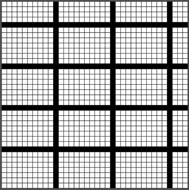
(a)

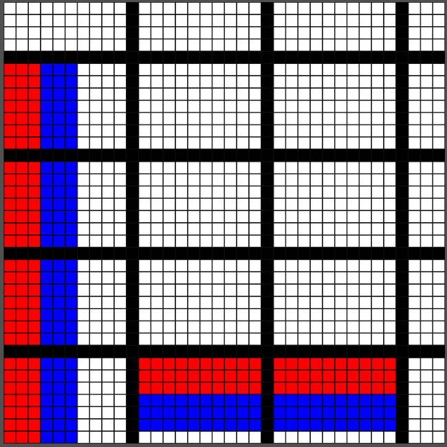
(b)

Figure 3: (a) An example of a stripes pattern. (b) The blue tiles count to the next stripe while the red tiles count the number of stripes.

4 Tight Bounds for Patterns on $n\times n$ Squares

In this section, we prove tight bounds on the tile complexity of self-assembling 2-colored patterns on the surfaces of $n\times n$ squares for almost all positive integers $n$.

Theorem 4.1

For almost all positive integers $n$, the tile complexity of weakly self-assembling 2-colored patterns on a $n\times n$ squares in the aTAM is $\Theta\left(\frac{n^{2}}{\log n}\right)$.

We prove Theorem 4.1 by separately proving the lower and upper bounds, as Lemma 1 and Lemma 2, respectively.

Lemma 1

For almost all positive integers $n$, the tile complexity of self-assembling a $2$-color pattern on an $N\times N$ square in the aTAM is $\Omega\left(\frac{n^{2}}{\log n}\right)$.

The proof of Lemma 1 is a straight-forward information-theoretic argument but we include it for the sake of completeness.

Proof

Let $\mathcal{T}=(T,\sigma,\tau)$ be a singly-seeded TAS such that $\tau\in\mathbb{Z}^{+}$ is a fixed constant, the strength of every glue of $T$ is bounded by $\tau$ and $B\subseteq T$ and assume $\mathcal{T}$ weakly self-assembles a 2-color pattern on an $n\times n$ square in the aTAM. In other words, every domain of $\mathcal{T}$ is an $n\times n$ square, and we may assume without loss of generality that the type of tile placed at every point therein is either “white” or “black”. Let $B\subseteq T$ be the subset of tiles of $T$ whose colors are “black”.

Let $n\in\mathbb{Z}^{+}$ and $w=w_{n^{2}-1}\cdots w_{0}\in\{0,1\}^{n^{2}}$. Define the pattern corresponding to $w$ as the set $P_{w}\subseteq\{0,\ldots,n-1\}^{2}$ such that for all $1\leq i<n^{2}$, $\left(i\mod n,\left\lfloor\frac{i}{n}\right\rfloor\right)\in P_{w}$ if and only if $w_{i}=1$. Let $P_{w}\subseteq\{0,\ldots,n-1\}^{2}$ and assume $\mathcal{T}_{w}$ weakly self-assembles $P_{w}$.It is easy to see that for every $n\in\mathbb{Z}^{+}$ and $w\in\{0,1\}^{n^{2}}$, there exists a TAS $\mathcal{T}_{w}=\left(T,\sigma,\tau\right)$ such that $\left|T\right|=O\left(n^{2}\right)$.

Going forward, let $n\in\mathbb{Z}^{+}$ and $w\in\{0,1\}^{n^{2}}$ be arbitrary and suppose $\mathcal{T}_{w}$ is the corresponding TAS that weakly self-assembles the pattern corresponding to $w$.

Note that $\mathcal{T}_{w}$ has $4\left|T_{w}\right|$ glues, each strength is bounded by $\tau$, which is a fixed constant, and every tile is either in $B$ or not. This means $\mathcal{T}$ can be represented using $O\left(\left|T_{w}\right|\log\left|T_{w}\right|\right)$ total bits. Let $\left\langle\mathcal{T}_{w}\right\rangle$ be such a representation of $\mathcal{T}_{w}$.

Let $w\in\{0,1\}^{*}$, and $U$ be a fixed universal Turing machine. The Kolomogorov complexity of $w$ is: $K_{U}(w)=\min\left\{\left|\pi\right|\mid U(\pi)=w\right\}$. In other words, $K_{U}(w)$ is the size of the smallest program that when simulated on $U$ outputs $w$. Let $m$ be a non-negative integer and $\varepsilon>0$ be a fixed real constant. The number of binary strings of length less than $m-\varepsilon m$ is at most $1+2+4+\cdots+2^{\lfloor m-\varepsilon m\rfloor-1}=2^{\lfloor m-\varepsilon m\rfloor}-1<2^{\lfloor m-\varepsilon n\rfloor}<2^{m-\varepsilon m+1}$. Define $A_{m,\varepsilon}=\left\{w\in\{0,1\}^{m}\mid K_{U}(w)\geq(1-\varepsilon)m\right\}$. Note that

$$\frac{\left|A_{m,\varepsilon}\right|}{2^{m}}\geq\frac{2^{m}-2^{m-\varepsilon m+1}}{2^{m}}=1-\frac{2^{m-\varepsilon m+1}}{2^{m}}=1-\frac{1}{2^{\varepsilon m-1}}.$$

Thus, we have

$$\lim_{m\rightarrow\infty}{\frac{\left|A_{m,\varepsilon}\right|}{2^{m}}}=1,$$

which means that if $\varepsilon>0$ is fixed, then for almost all strings, $w\in\{0,1\}^{m}$, $(1-\varepsilon)n<K_{U}(w)$.

There exists a fixed program $\pi_{SA}$ that takes as input $\langle\mathcal{T}_{w}\rangle$, simulates it, and outputs the string $w$ that corresponds to the pattern $P_{w}$ that $\mathcal{T}_{w}$ self-assembles. Then, for almost all strings $w\in\{0,1\}^{n^{2}}$,

$$(1-\varepsilon)|w|<K_{U}(w)<C_{1}\left(\left|\pi_{SA}\right|+\left|T_{w}\right|\log\left|T_{w}\right|\right)<C_{2}\left|T_{w}\right|\log|w|.$$

It follows that $\left|T_{w}\right|=\Omega\left(\frac{|w|}{\log|w|}\right)=\Omega\left(\frac{n^{2}}{\log n^{2}}\right)=\Omega\left(\frac{n^{2}}{\log n}\right)$.

Since $n$ and $w$ were arbitrary, the lemma follows.

To prove the lower bound for Theorem 4.1, we prove the following, which is a stronger result that applies to all positive integers $N$.

Lemma 2

For all positive integers $N$, for every pattern $P\subseteq\{0,\ldots,N-1\}^{2}$, there exists an aTAM system $\mathcal{T}=(T,\sigma,1)$ such that $|\sigma|=1$, $|T|=O\left(\frac{N^{2}}{\log N}\right)$ and $\mathcal{T}$ weakly self-assembles $P$.

Proof

We proceed by construction. Let $N\in\mathbb{Z}^{+}$ be the dimensions of the square and $P$ be the $N\times N$ pattern of black and white pixels to weakly self-assemble on the square. Our construction will yield a system $\mathcal{T}=(T,\sigma,1)$ that self-assembles an $N\times N$ square on which $P$ is formed by the black and white tiles of $T$. The tile set $T$ will be composed of two subsets, $T_{s}$ whose tiles form the skeleton, and $T_{r}$ whose tiles form the ribs. We first explain the formation of the skeleton, then that of the ribs. Figure 4 shows a high-level depiction. Throughout our discussion, we will use the notation $P(x,y)$ to denote the color (black or white) of the pattern $P$ at location $(x,y)$.

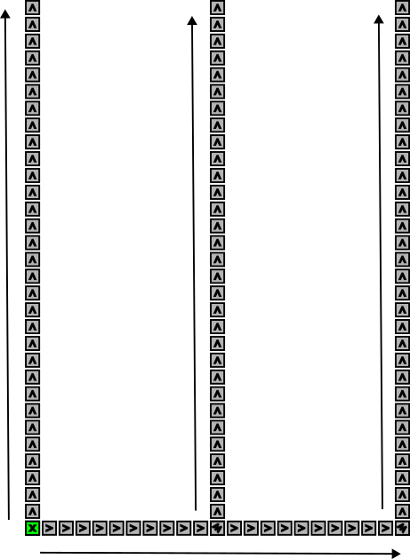
(a) The skeleton. The seed is represented in green in the lower left and the arrows show the directions of growth.

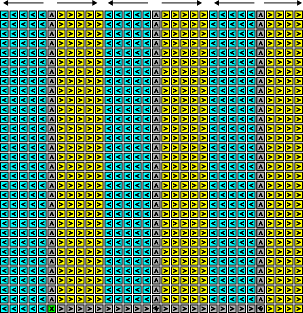
(b) The square once the ribs of the skeleton have filled in (blue growing left, yellow growing right)..

Figure 4: A schematic example of the construction of the proof of Theorem 2. Instead of showing the black and white colors corresponding to the pattern, we color the tiles to show the pieces of the construction to which they belong.

Skeleton
The seed is part of the skeleton and is placed at location $(\lfloor\log N\rfloor,0)$ and is given the same color as $P(\lfloor\log N\rfloor,0)$. Since a vertical column of the skeleton has width one, and the ribs growing off of each side have length $\lfloor\log N\rfloor$, the width of a pair of ribs and its skeleton column (which we will call a rib-pair) is $2\lfloor\log N\rfloor+1$. Dividing the full width $N$ by the width of a rib-pair, and taking the floor, gives the number of full rib-pairs that will fit. Let $f=\lfloor\frac{N}{2\log N+1}\rfloor$ be this number. Let $r=N\mod(2\lfloor\log N\rfloor+1)$ be the remaining width after the last full rib-pair. If $r<\lfloor\log N\rfloor+1$, then a column of the skeleton grows up immediately to the right of the last full rib-pair, and its ribs are of length $r-1$ and grow to the right. If $r\geq\lfloor\log N\rfloor+1$, then the last skeleton column grows upward $\lfloor\log N\rfloor$ positions to the right of the last full rib-pair and has full-length ribs (i.e., $\lfloor\log N\rfloor$) that grow to its left and ribs of length $r-(\lfloor\log N\rfloor+1)$ grow to its right. In the first case, the row of the skeleton that forms the bottom row of the square extends from the seed to $x$-coordinate $f(2\lfloor\log N\rfloor+1)+1$. In the second case, that row extends from the seed to $x$-coordinate $f(2\lfloor\log N\rfloor+1)+\lfloor\log N\rfloor+1$. The tiles of that row are hard-coded and there are $O(N)$ of them. Starting with the seed and then occurring at every $2\lfloor\log N\rfloor+1$ locations of the bottom row, a hard-coded set of tiles grows a column of height $N-1$. This row and set of columns are the full skeleton. The number of tile types is $O(N)$ for the row and $O(N)$ for each of the $O\left(\frac{N}{\log N}\right)$ columns, for a total of $O(N)+O\left(\frac{N^{2}}{\log N}\right)=O\left(\frac{N^{2}}{\log N}\right)$ tile types. Note that each skeleton tile type is given the color of the corresponding location in the pattern $P$.

Ribs
From the east and west sides of each location on the columns of the skeleton, ribs grow. Each rib is composed of $\lfloor\log N\rfloor$ tiles (except the ribs growing from the easternmost column, which may be shorter). Since there are two possible colors for each of the $\lfloor\log N\rfloor$ locations of a rib, there are a maximum of $2^{\lfloor\log N\rfloor}\leq N$ possible color patterns for any rib to match the corresponding locations in $P$. (Note that we will discuss the construction of the tiles for ribs that grow to the east, and for ribs that grow to the west the directions are simply reversed.) For any given rib $r$, let the portion of $P$ corresponding to the locations of $r$ be represented by the binary string of length $\lfloor\log N\rfloor$ where each black location is represented by a $0$, and each white by a $1$. For example, for a rib $r$ of length $5$ growing eastward from a column, if the corresponding locations of $P$ are “black, black, white, black, white”, then the binary string will be “$00101$”. For each possible binary string $b$ of length $\lfloor\log N\rfloor$, i.e. $b\in\{0,1\}^{\lfloor\log N\rfloor}$, a unique tile type, $t_{b}$, is made. with the glue $b$ on its west side and the glue $b[1:]$ (i.e. $b$ with its left bit truncated) on its east side. This tile type is given the color corresponding to the first bit of $b$. Additionally, for each skeleton column tile from which a rib should grow to the east with pattern $b$, the glue $b$ will be on its east side, allowing $t_{b}$ to attach. This results in the creation of a maximum of $N$ unique tile types (and there will be another $N$ for the first tiles of each westward growing rib). Recall that the tile types for the skeleton were already accounted for and each is hard-coded so that the placement of these glues does not require any new tile types for the skeleton.

Now, the process is repeated for each binary string from length $b-1$ to $1$, with the color of each tile being set to the value of the first remaining bit. Each iteration requires half as many tile types to be created as the previous, i.e. $2^{\lfloor\log N\rfloor-1}$, then $2^{\lfloor\log N\rfloor-2}$, $\ldots$, $2$. Intuitively, each rib position has glues that encode their bit value in the pattern and the portion of the pattern that must be extended outward from them, away from the skeleton. Therefore, for the last position on the tip of each rib, there are exactly 2 choices, white or black, and so all ribs share from a set of two tile types made specially for the ends of ribs. For the tile types of ribs that grow to the east, the total summation is $\Sigma^{\log N-1}_{x=0}{2^{\log N-x}}=2N-2=O(N)$. Accounting for the additional tile types needed for west growing ribs, the full tile complexity of the ribs is $O(N)$.

Thus, the total tile complexity for the tile types of the skeleton plus those of the ribs is $O\left(\frac{N^{2}}{\log N}\right)+O(N)=O\left(\frac{N^{2}}{\log N}\right)$.

Correctness of construction
The system $\mathcal{T}$ designed to weakly self-assemble $P$, as discussed, has a seed of a single tile, and since all tile attachments require forming a bond with a single neighbor, the temperature of the system can be $\tau=1$. Our prior analysis shows that the tile complexity is correct at $O\left(\frac{N^{2}}{\log N}\right)$, and showing that $\mathcal{T}$ weakly self-assembles $P$ is trivial since (1) the tiles of the skeleton are specifically hard-coded to be colored for their corresponding locations in $P$, and (2) for each possible pattern corresponding to a rib there is a hard-coded set of rib tiles that match that pattern and grow from the skeleton into that location. Thus, $P$ is formed and Lemma 2 is proved, and with both Lemmas 1 and 2, Theorem 4.1 is proved.

5 Repeated Patterns

In this section we discuss repeated patterns and show constructions of how to repeat any pattern.

Definition 4 (Grid Repeat Pattern Class)

We define a pattern class that given a 2-colored pattern $p_{i}$ and a $m$ will create new pattern $p_{0}$ that tiles $p_{i}$ $m$ times vertically and horizontally forming a grid of the pattern.

$GRID\_REPEAT:(p_{i},m)\rightarrow p_{o}$ where

• $m\in\mathbb{N}$

• $p_{i}\in SQPATS_{n}$

• $p_{o}\in SQPATS_{n*m}$

• $p_{o}$ is constructed by making an $m\times m$ grid of $p_{i}$ patterns

Theorem 5.1 (Repeated Pattern Tile Complexity)

For all $n,m\in\mathbb{N}$, and $P\in SQPATS_{n}$ there exists an aTAM system $\mathcal{T}=(T,\sigma,2)$ such that $|\sigma|=1$, $|T|=O(\frac{n^{2}}{\log{n}}+\log{mn})$ and $\mathcal{T}$ strictly self-assembles $GRID\_REPEAT(P,m)$.

Proof

We will prove the theorem by presenting a construction for $GRID\_REPEAT$ and showing that all produced aTAMs have $O(\frac{n^{2}}{\log{n}}+\lg{nm})$ tiles.

Let $\mathcal{T}_{P}$ be a TAS that strictly self assembles $P$ using the skeleton construction from 4.1. We will use this assembly as a sub component of the larger assembly that builds $GRID\_REPEAT(P,m)$. We divide the skeleton into $\frac{n}{\log n}$ parts called spines. Each spine is the vertical bar that extends upwards (the shaft) and a subsection of bottom row of the skeleton extending as far as the ribs that connect to the spine (the base). The skeleton construction will also be modified to use temp 2 and have the bottom row extend the length of the full square. This does not change the tile complexity of the construction.

Now we present the construction. Given a pattern $P$ and an integer $m$ a TAS $\mathcal{T}_{R}$ is built. Let $T_{COUNT}$ be a constant set of counter tiles. For each tile in $T_{COUNT}$ we create a copy of each spine from $\mathcal{T}_{P}$. The new spine will have the glues from the counter tile appended to the north of the shaft and the south, east, and west ends of the base. A copy of the rib tiles will also be made that has the counter tile’s north glue appended to their glue. This allows for the entire spine to be constructed and other spines to grow off of it according to the growth of the counter tiles. We repeat this process again to create a version of $\mathcal{T}_{P}$ where the structure is rotated 90 degrees so it grows to the east, but the pattern is still facing upwards. This will grow to the east end of the square.

Then another copy of the tiles from $\mathcal{T}_{P}$ is added to fill in the rest of the square with the pattern. There are a constant number of copies of $\mathcal{T}_{P}$ in the assembly so the tile complexity of these sections is the tile complexity of building any square pattern. The 4.1 theorem showed this to be $O(\frac{n^{2}}{\log n})$.

The seed of $\mathcal{T}_{R}$ will embed the starting value of the counter such that it counts $m$ times before it stops. This means that $\log m$ spines will be needed to encode the starting value. Only the bases of the spines will need to be hard coded in the seed. The bases are $\log{n}$ tiles long, so the seed will need to be a hard coded $\log nm$ tile types. If $\log m>\frac{n}{\log n}$ then the seed will span multiple copies of $P$. The seed will also travel upwards to set the starting counter value for the rotated section of the assembly.

Correctness of construction
The construction outputs a TAS $\mathcal{T}_{R}$ that is designed to strictly self-assemble $GRID\_REPEAT(P,m)$ for all patterns and values of $m$. It has a seed of a single tile and grows the entire skeleton from it. Our prior analysis shows that the tile complexity is correct at $O(\frac{n^{2}}{\log n}+\log{nm})$. Thus 5.1 is proved.

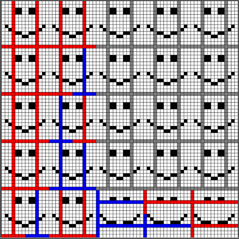
Figure 5: An example of an assembly that repeats a pattern $m=5$ times horizontally and vertically. Each spine is colored solely for clarity of presentation and in the actual construction the colors of the tiles on the spines would match the pixels of the pattern. Red spines represent a 1 and blue spines represent a 0. The spines count upwards until the counter is finished

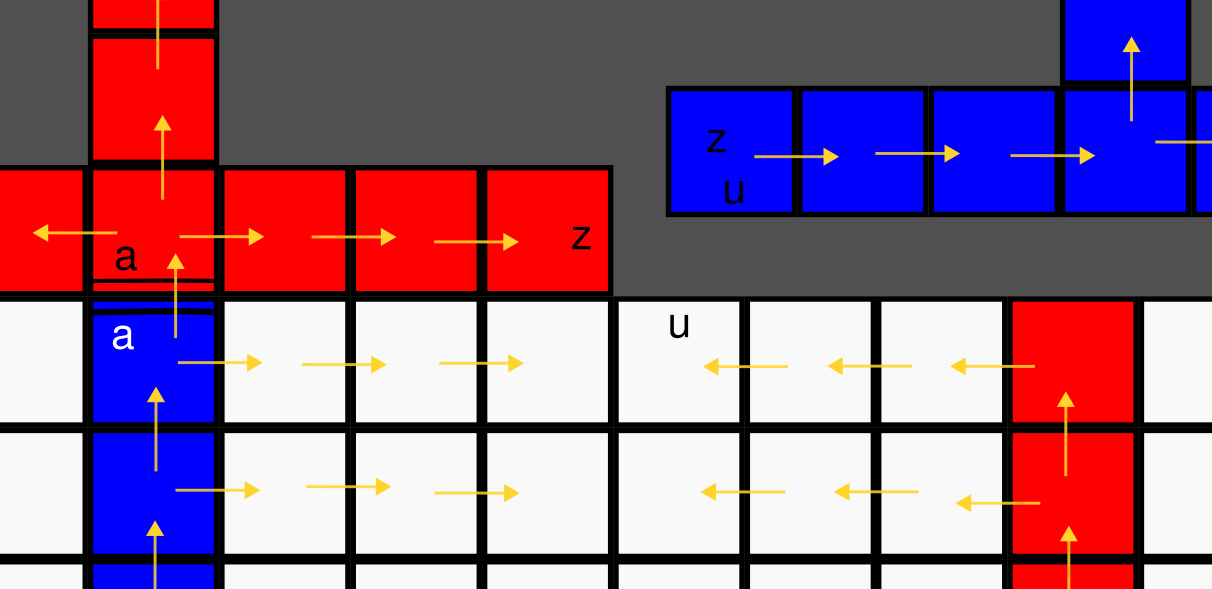
Figure 6: An example of how the binding of a spine works. The arrows indicate the growth of the tiles. The letter indicate glues. In this example, after the blue spine at the bottom finishes growing it can grow the next red spine. The incoming blue spine tiles cooperatively binds with this red spine and the ribs from the spine below. This tile will grow the rest of the spine and the pattern continues.

6 Multilayered patters

In this section, we prove that there exist patterns, both finite and infinite, that can be weakly self-assembled using asymptotically fewer tile types by barely-3DaTAM systems than by regular, 2D aTAM systems.

Theorem 6.1

For all $n\in\mathbb{Z}^{+}$, for some $m\in\mathbb{Z}^{+}$ there exists a 7-colored $m\times m$ pattern, $p_{n}$, such that no aTAM system $\mathcal{T}_{\leq n}=(T,\sigma,\tau)$ where $|T|\leq n$, $|\sigma|=1$, and $\tau\leq 2$ weakly self-assembles $p_{n}$, but a barely-3DaTAM system $\mathcal{T}_{p_{n}}=(T_{p_{n}},\sigma_{p_{n}},2)$ where $|T_{p_{n}}|=O(\log{n}/\log{\log{n}})$ and $|\sigma_{p_{n}}|=1$ weakly self-assembles $p_{n}$.

Proof

We prove Theorem 6.1 by giving the details of such a pattern $p_{n}$ that consists of a repeating “grid” of 7-colored lines on the surface of an $m\times m$ square, for $m\in\mathbb{Z}^{+}$ to be defined, and a barely 3D aTAM system $\mathcal{T}_{p_{n}}=(T_{p_{n}},\sigma,2)$ that weakly self-assembles $p_{n}$, with the tiles in $z=1$ colored in the pattern of $p_{n}$, and $|T_{p_{n}}|=O(\log{n}/\log{\log{n}})$ tile types. We show that every 2D aTAM system $\mathcal{T}_{\leq n}$ with fewer than $n$ tile types fails to weakly self-assemble $p_{n}$ by constructing $p_{n}$ so that it differs, in at least one location in each “cell” of a repeating grid of cells, from an assembly producible in each $\mathcal{T}_{\leq n}$. Two different examples of such patterns can be seen in Figure 7. A pattern $p_{n}$ consists of an $m\times m$ square that is covered in a repeating grid of square “cells.” Each cell is a $c\times c$ square where the north row and west column of each is considered “boundary,” and the rest of each cell is considered “interior.” The easternmost column and the southernmost row of cells may consist of truncated cells depending on the values of $m$ and $c$ (i.e., if $m\mod c\neq 0$). Since each cell contributes a north and west boundary, each cell interior is completely surrounded by boundaries (except, perhaps, the easternmost column and southernmost row). Depending on a bit sequence specific to each $p_{n}$ (to be discussed), the set of colors of the boundaries will be either $\{\texttt{White},\texttt{Green},\texttt{Black}\}$ or $\{\texttt{Red},\texttt{Green},\texttt{Black}\}$. The set of colors of the interiors will be $\{\texttt{Aqua},\texttt{Blue},\texttt{Yellow}\,\texttt{Fuchsia}\}$. Thus, each pattern $p_{n}$ will be composed of 7 colors.

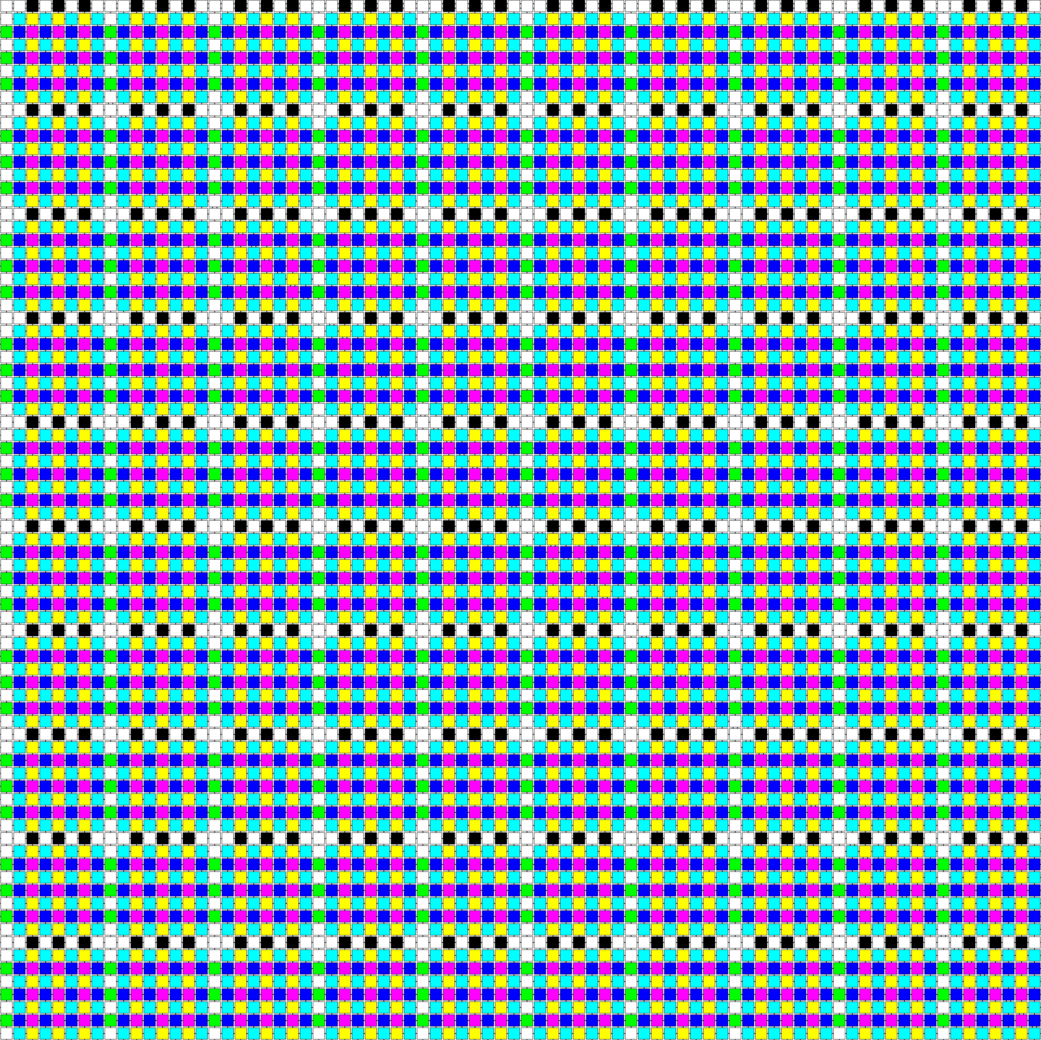
(a) Example grid pattern for bit sequence $11010101$.

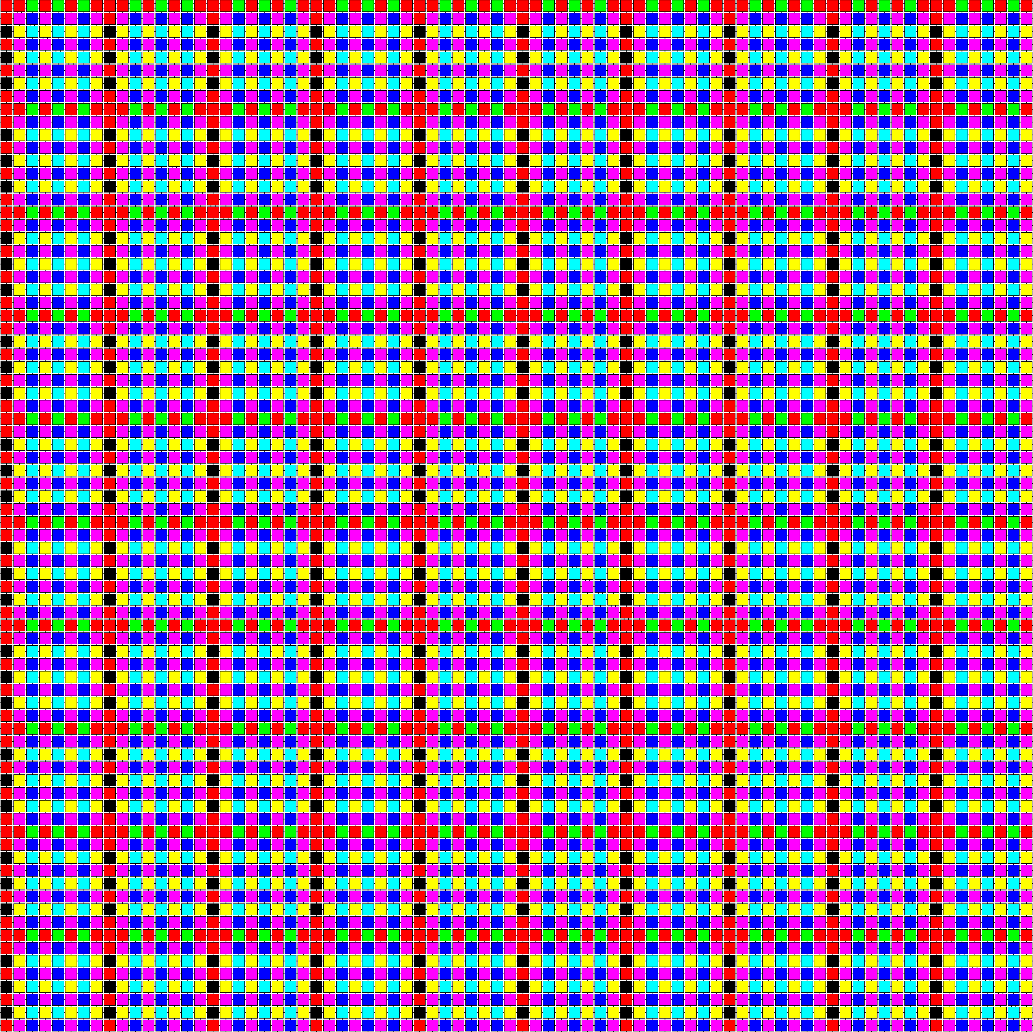
(b) Example grid pattern for bit sequence $00101010$.

Figure 7: Example $p_{n}$ patterns created by the construction in the proof of Theorem 6.1. The (repeatedly copied) binary sequence of results from the simulations of aTAM systems starts at the top, with the two colors of that row, and all subsequent boundary rows, being determined by the first bit of that pattern. During the downward growth from that row, during which a full square is formed, the repeating grid formed by the copies of that pattern is copied both downward and to both sides. The boundary columns also have two colors determined by the first bit of the sequence (one of them the same as in the boundary rows) for a total of 3 boundary colors. The interiors always use the same 4 colors.

The bit sequence that determines the colors used by the boundaries, and the ordering of the colors on the boundaries and in the interiors, is determined via simulations of a series of aTAM systems. Intuitively, our proof utilizes a construction that performs a diagonalization against all possible aTAM systems with $\leq n$ tile types by simulating each, and for each keeping track of the color of tile it places in a location specific to the index of that system so that it can ultimately generate the colored pattern $p_{n}$ that differs in at least one location from every simulated system. The dimensions of each $c\times c$ cell are $c=T(n)$, where $T(n)$ is a function that takes a number of tile types and returns a count of all possible aTAM systems with $\leq n$ tile types (with the caveat that it “overcounts” by allowing for functionally duplicate systems, as this does not impact the correctness and makes the discussion of the proof simpler). The colors of the rows and columns encode the bit sequence generated by the simulations, with the same bit sequence encoded in both the rows and the columns via an assignment of colors. There is a unique color assigned for each intersection of two bits (i.e. 00, 01, 10, and 11), with 4 colors reserved for boundaries of grid cells and 4 separate colors reserved for the interior locations of the grid cells.

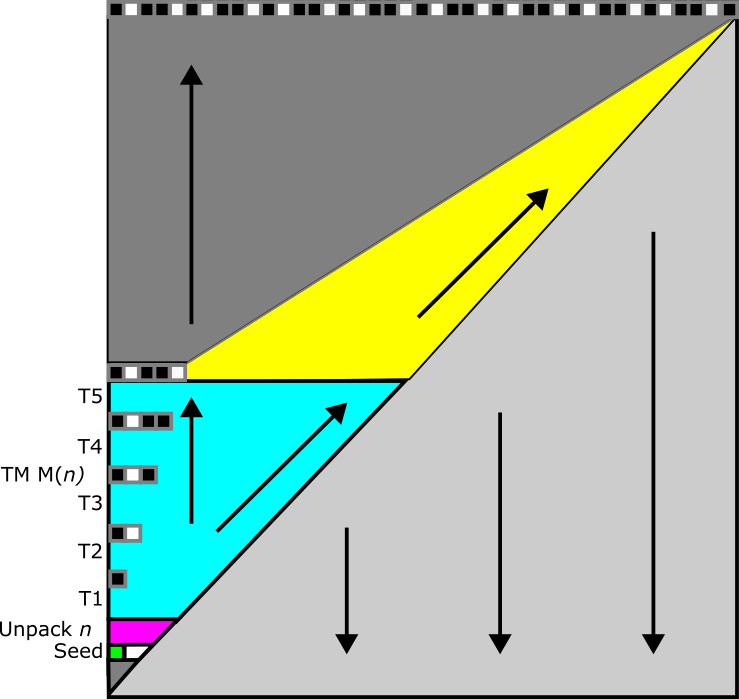
Figure 8: Schematic overview of the portion of the construction for the proof of Theorem 6.1 that grows in plane $z=0$. Note that the modules are not shown to scale. (Green) The seed tile, (Fuchsia) the base conversion module that unpacks the binary representation of $n$, (Aqua) the module that simulates the Turing machine $M$ on input $n$, that in-turn simulates each TAS with $\leq n$ tile types in sequence and saves a result bit (Black or White) for each, (Yellow and Grey) the pattern of result bits is copied repetitively to the right until it covers the entire top row. (Light Grey) A simple “filler” tile causes the assembly to form a complete square.

At a high-level, the construction consists of a handful of components (of varying complexity) that can be seen schematically depicted in Figure 8. The number $n$ is encoded in $O(\log{n}/\log{\log{n}})$ tile types following the technique of [1]. From the seed tile of $\mathcal{T}_{p_{n}}$, the $O(\log{n}/\log{\log{n}})$ tiles representing $n$ in an optimally compressed base grow to the right. Then, rows grow upward and to the right to do a base conversion in which the bits of $n$ are “unpacked” so that the northern glues of the tiles of top row of that triangle represent $n$ as $\log{n}$ bits (shown in fuchsia in Figure 8). (Figure 9 depicts a slightly more detailed example of the bit unpacking.) A simple set of filler tiles grow to the south of the seed’s row to form the bottom of the triangle. The tile complexity of this stage of the construction is $O(\log{n}/\log{\log{n}})$. The tile complexity of the remaining portions of the construction is $O(1)$, as they use a constant number of tile types independent of $n$.

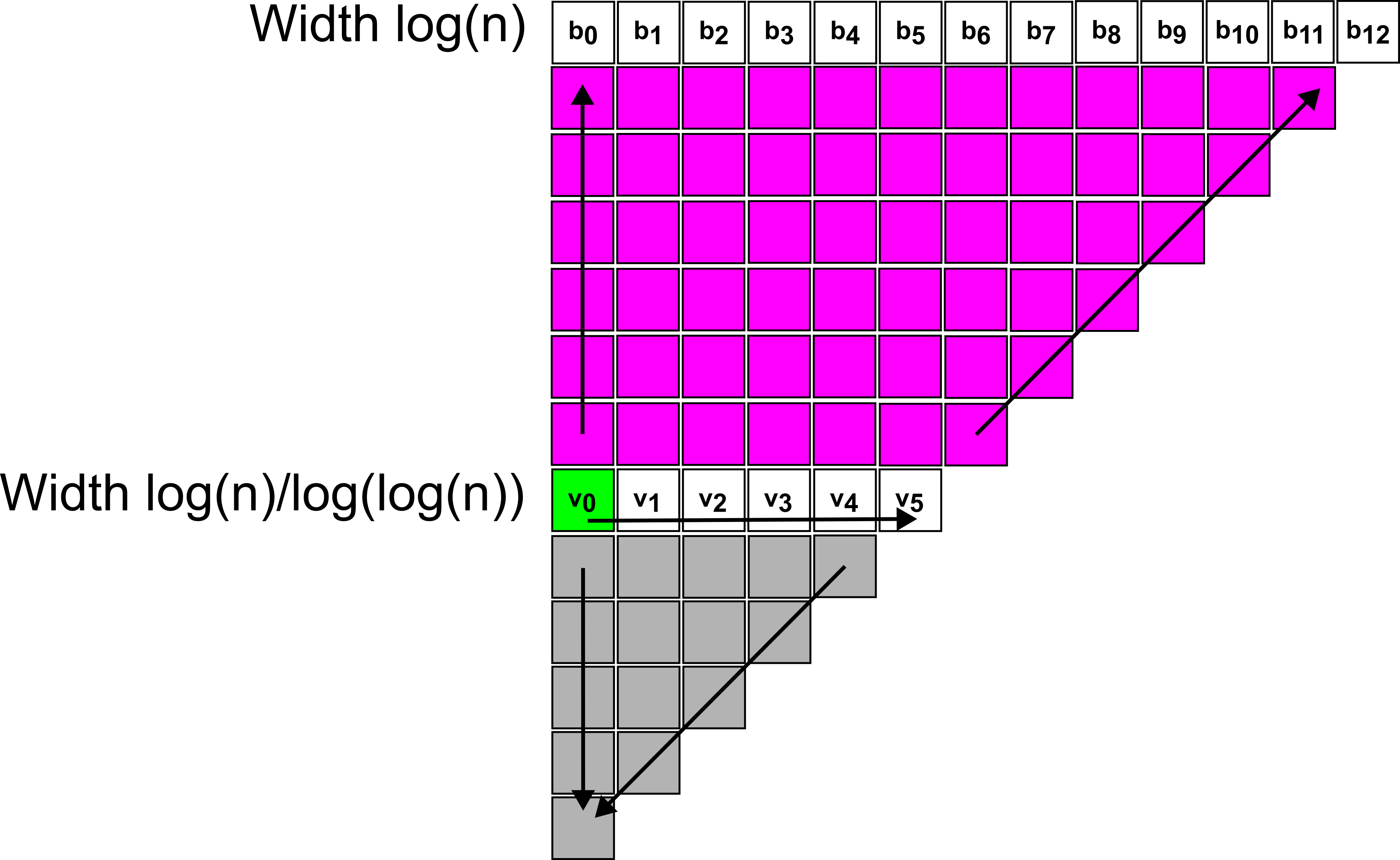
Figure 9: Schematic example of the growth of the base conversion module’s growth from Figure 8. The seed tile is shown in green. Using the technique of [1], the number $n$ is encoded using $O(\log{n}/\log{\log{n}})$ tile types. These tile types form the (white) row that grows to the east of the seed. A base conversion then occurs via rows that grow to the north (fuchsia) to convert $n$ to binary, so that the northern row of this module (white) consists of tiles that encode $n$ in binary.

6.1 Simulation of all aTAM systems with $\leq n$ tile types

A zig-zag Turing machine module (i.e., a standard aTAM construction in which a growing assembly simulates a Turing machine while rows grow in alternating, zig-zag, directions and each row increases in length by one tile - see [10, 7, 2] for some examples) uses $n$ as input. The Turing machine $M$ being simulated runs the procedure SimulateAllTileAssemblySystems, with argument $n$, as shown in Algorithm 1 (and depicted in aqua in Figure 8).

SimulateAllTileAssemblySystems is given the number $n$ as the maximum number of tile types allowed in a system, and first uses that to compute the number of all possible aTAM tile sets that could be created with up to $n$ tile types. The number of possible glues for each side of a tile (recognizing that having more glue labels than tile types is equivalent to having glues with no binding partners, which is equivalent to making those unmatched glues null) is $O(n)$, and with 8 possible colors and 4 sides for any tile type, the number of possible tile types is $O(n^{4})$. To determine all possible aTAM systems that could be made from this set of possible tile types, we overcount (since it does not change the correctness and it makes the analysis and proof easier to follow) as $O((n^{4})^{n^{4}})=O(n^{4n^{4}})$. Note that this accounts for all tile sets of size $\leq n$ since one of the tile types is the null tile type with no glues (which can simply be omitted from any set without changing its behavior) while also counting many identical (i.e. functionally equivalent) tile sets multiple times. Additionally, while all of the simulations will be at temperature $\tau=2$, since all possible tile sets will be generated with only strength-2 glues, and when simulated at $\tau=2$ these are functionally equivalent to tile sets where the glues are changed to strength-1 and simulated at $\tau=1$, this method of counting causes the behaviors of all possible systems with $\leq n$ tile types and $\tau\leq 2$ to be simulated (again, many of them multiple times).

To generate all possible aTAM systems with single-tile seeds from that collection of possible tile sets, since we can keep the temperature at $\tau=2$ (as previously explained), we only need to vary the tile types that serve as the seed (because we only consider systems with single-tile seeds). Creating a unique system for each tile type in a tile set to be the seed yields $O(n*n^{4n^{4}})=O(n^{4n^{4}+1})$ aTAM systems. For simplicity, we refer to this value as $T(n)$ (as previously mentioned). Since each of the $T(n)$ systems will be simulated and a bit value will be saved for each (ultimately allowing the construction to build a pattern $p_{n}$ that differs from each of them), that bit sequence will be of length $T(n)$. We will use the value of $T(n)$ to determine the number of steps for which each system must be simulated.

Recall that $p_{n}$ consists of a grid of cells of size $T(n)\times T(n)$ repeated horizontally and vertically. As each system $\mathcal{T}_{i}$, for $0<i\leq T(n)$, is simulated, its index $i$ is noted so that the construction can guarantee that the $i$th row and $i$th column of each cell will differ from a (potentially) corresponding location in the assembly produced by $\mathcal{T}_{i}$ during its simulation. We want to ensure that for each $\mathcal{T}_{i}$, if it happens to make a repeating grid of $T(n)\times T(n)$ cells composed of 7 colors, $p_{n}$ differs in at least one location of each cell from at least one location of one cell of the pattern produced by $\mathcal{T}_{i}$. Any system $\mathcal{T}_{i}$ that does not even produce a single valid cell of size $T(n)\times T(n)$ bounded by the boundary colors has no chance of generating $p_{n}$ so can be easily discounted. For all other $T_{i}$, a bit computed after running the simulation of $T_{i}$ is used to ensure $p_{n}$ differs.

6.2 Making $p_{n}$ differ from each simulated system

For the simulation of each system, we do not impose a restriction upon the translation of the pattern that the system makes relative to our target pattern $p_{n}$. Therefore, we cannot assume the relative position of the seed tile of $\mathcal{T}_{i}$ with respect to any portion of $p_{n}$, and we simulate each $\mathcal{T}_{i}$ until it grows an assembly that has at least one dimension (width or height) that spans the distance of a full cell with boundaries on both sides. To do so, we simulate each $\mathcal{T}_{i}$ for $4T(n)^{2}$ steps because this is the number of tiles contained within a $2\times 2$ square of grid cells, ensuring that irrespective of the position of the seed tile with respect to the pattern formed, the full dimension of at least one grid cell and its boundaries in that dimension must be spanned. Figure 10 shows an example of grid cells and a bounding box of that size, demonstrating why such bounds suffice. (Note that any system that becomes terminal before reaching such a size clearly cannot weakly self-assembly $p_{n}$, since it is much larger, so we can record an arbitrary output bit for that simulation.) Since we are only concerned with systems that can create grid-like patterns with the same boundary and interior colors used by $p_{n}$ (as differing patterns created by other systems will immediately disagree with $p_{n}$), we can inspect the assembly $\alpha_{i}$ produced by the simulation of $\mathcal{T}_{i}$ as follows.

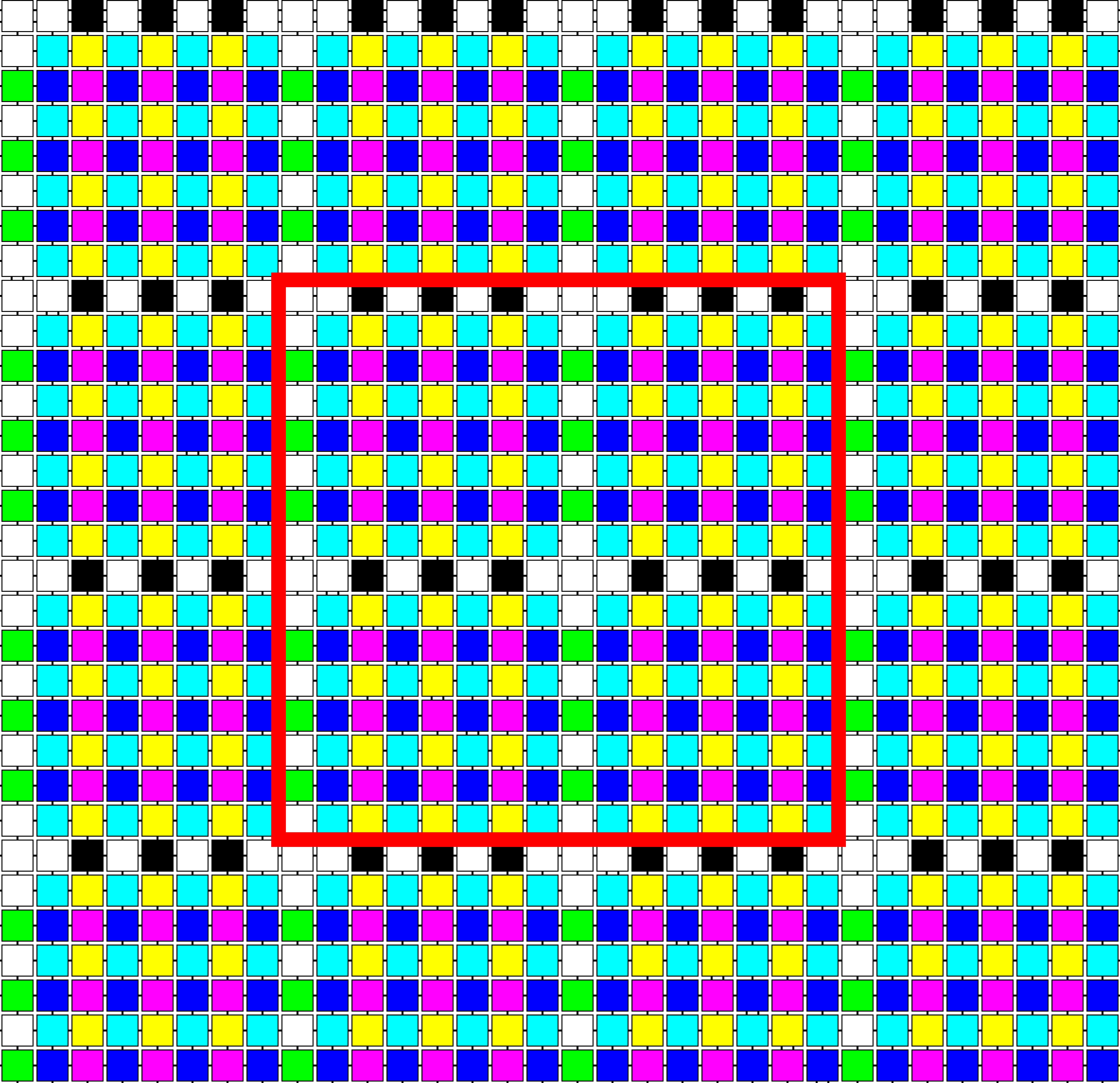
Figure 10: A portion of a pattern $p_{n}$ for the bit sequence $11010101$, showing a $4\times 4$ grid of cells and a bounding box (Red) enclosing a $2\times 2$ portion of the grid, containing $4T(n)^{2}$ tiles, where $T(n)$ is the width and height of a cell. Any assembly containing $4T(n)^{2}$ tiles must contain a connected component of at least width $\geq T(n)+1$ and/or height $\geq T(n)+1$, ensuring two boundary locations on the sides of an assembly spanning a cell.

Without loss of generality, assume that $\alpha_{i}$ has width $\geq 2T(n)$. If not, it must have height $\geq 2T(n)$ and the algorithm searches from north to south instead of west to east as described below. Starting from any leftmost tile of $\alpha_{i}$, we inspect its color and continue inspecting the colors of tiles one position to the east of the previous, looping until we encounter one whose color is a boundary color. (A simple example can be seen in Figure 11.) At that point, we skip an additional $i$ tiles to the east (noting that the $y$-coordinates don’t matter, only the $x$-coordinates). Once a tile is found at that $x$-coordinate, which is guaranteed by the number of tiles in $\alpha_{i}$ and the assumption that its width (rather than height) is $\geq 2T(n)$, its color is noted. The pattern $p_{n}$ will be produced so that the colors of each column represent a bit, 0 or 1, and the colors of each row represent a bit, 0 or 1. For the locations of a boundary row or column, there are 4 possible colors ($\{\texttt{White},\texttt{Green},\texttt{Black},\texttt{Red}\}$) used to represent the intersection of each location’s row and column value, i.e., 00, 01, 10, and 11. For the other (a.k.a. interior) locations, a set of 4 different colors is used ($\{\texttt{Aqua},\texttt{Blue},\texttt{Yellow}\,\texttt{Fuchsia}\}$). Indexing each row and column by $0<i\leq T(n)$ allows the $i$th row and $i$th column of each grid cell to be associated with a bit value. The bit value chosen to be saved is determined by the analysis of the color of the tile at index $i$ in $\alpha_{i}$ (i.e., the tile at an $x$-coordinate that is $i$ greater than that of a tile with a boundary color). If the color of the tile there is one of the two colors associated with a boundary row representing a 0, or one of the two colors associated with an interior row representing a 0, the bit value 1 is saved for that simulation. Otherwise, the bit value 0 is saved. When the pattern $p_{n}$ is later produced, it will use colors associated with this “flipped” bit for all rows and columns at index $i$ of all cells of the grid. Therefore, every tile of $p_{n}$ that is $i$ locations to the east of any tile with a boundary color will have a different color than the tile of $\alpha_{i}$ that is $i$ positions to the east of a tile with a boundary color. In this way, the pattern produced by $T_{i}$ cannot be $p_{n}$.

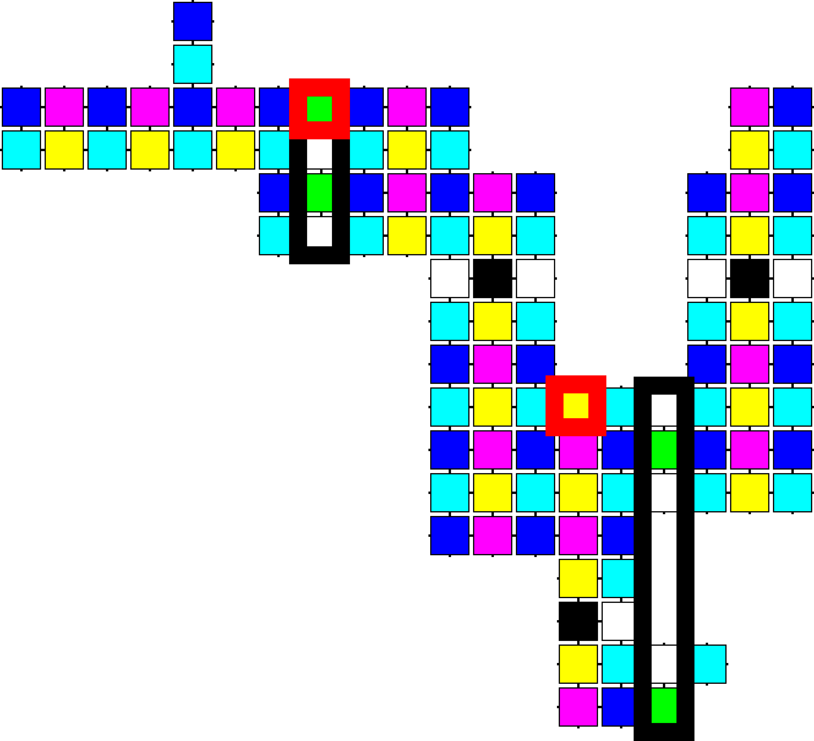
Figure 11: An example assembly $\alpha_{i}$ possibly formed during the simulation of some $T_{i}$. The leftmost red square hightlights a leftmost tile with a boundary color, and the corresponding black rectangle highlights the rest of that column and thus the boundary of a (potential) cell. Assuming $T(n)=8$, i.e., grid cell sizes of 8, the rightmost black rectangle highlights the locations of tiles at the boundary of the next cell to the right. Assuming an index value of $i=6$, the rightmost red square highlights a tile at that index, with respect to the boundary to the left. The color of the highlighted cell is Yellow, which is one of the two colors reserved for columns representing the bit value 0. Therefore, the bit value 1 is saved for index $i$ to ensure that the pattern $p_{n}$ will never place a Yellow tile $i$ locations to the east of a tile with a boundary color, guaranteeing that $p_{n}$ differs from the pattern produced by $T_{i}$.

The simulation of $M$ proceeds through the simulation of each of the $T(n)$ aTAM systems with $\leq n$ tile types. As the rows representing each simulation grow, they pass the currently computed sequence of bits upward through the tiles performing the simulations. Once $M$ completes, the sequence of generated bits is encoded in the north glues of the leftmost $T(n)$ tiles of the top row. This is represented in Figure 8 as the Black and White sequence on the top of the aqua-colored portion of the wedge. Note that the tile types that simulate $M$ are a constant-sized tile set, regardless of the value of $n$.

At that point, another constant-sized set of tiles grow in a zig-zag manner to copy the bit sequence over and over, to the right, until the entire top row consists of copies of the bit sequence (with the last copy of the sequence potentially truncated). Note that during all of the diagonal upward growth, a single “filler” tile type attaches to the right of the diagonal so that once the northward growth completes the full assembly will be a square.

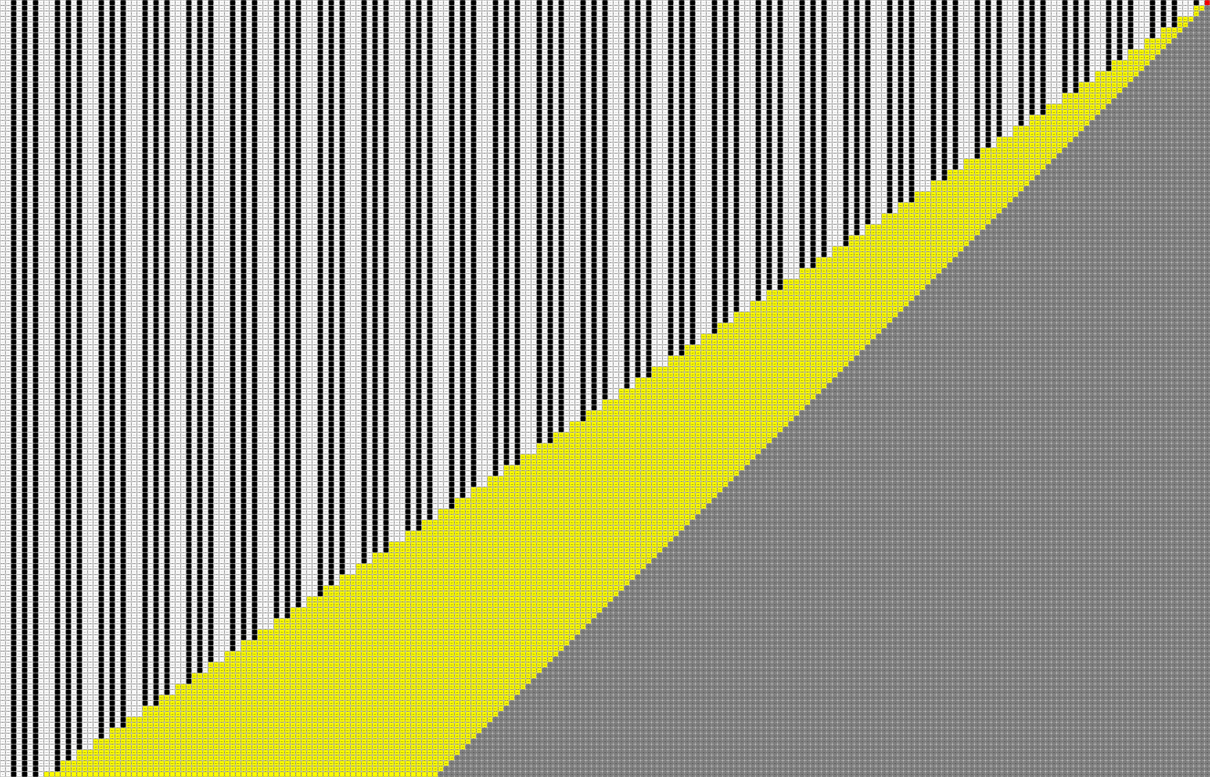
Figure 12: An example portion of the assembly from the proof of Theorem 6.1 that shows the copying of the bit sequence $11010101$ to the right until it occupies the entire top row. This corresponds to the portion of the construction shown in Figure 8 above the aqua portion. At the completion of the bit sequence copying, the rightmost tile of the topmost row (shown here in red), initiates the growth into the second plane in which the pattern $p_{n}$ will assemble. The grey portion below the yellow is formed by a single “filler” tile that causes the final assembly to be a square.

Once the bit sequence has been copied across the entire northern row, the final phase of the construction begins. The easternmost tile to attach to the top row has a strength-2 glue in the $+z$ direction, initiating growth of the second plane, onto which the pattern $p_{n}$ self-assembles. The first row to grow in $z=1$ is immediately above the northernmost row of the assembly at $z=0$ and cooperates with the tiles of that row to read the repeated bit sequence. This row forms the northern boundary row of all of the cells of $p_{n}$, and thus the tiles have the boundary colors. The northernmost row in $z=0$ grows from the left to the right and includes information about the first (i.e., leftmost) bit of the bit sequence. If the first bit of the sequence is 0, the first row in $z=1$, which is a boundary row, contains the two boundary colors for a row of value 0, which are $\{\texttt{Red},\texttt{Green}\}$. Otherwise, it contains the two boundary colors for a row of value 1, which are $\{\texttt{White},\texttt{Black}\}$. If it was 0 (resp. 1), then as that first row in $z=1$ grows from right to left, when it cooperates with a tile representing 0 in $z=0$ it will be colored Red (resp. White), When cooperating with a tile representing a 1, it will be colored Green (resp. Black).

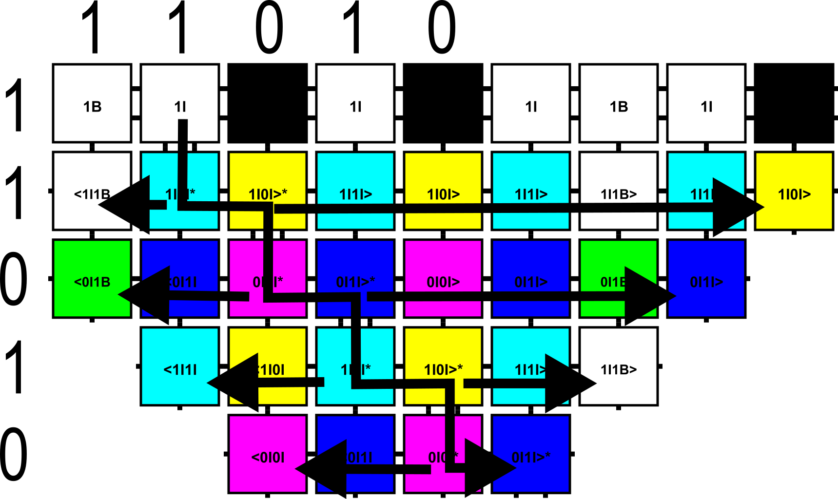
Figure 13: The growth of the grid, forming pattern $p_{n}$, from the topmost row, which is the initial row in plane $z=1$. The first tile placed in each row follows a diagonal path starting from the second tile from the left. Growth of each row expands left and right from the tile along the diagonal. The bit value for each column is propagated south from the top column, and the bit value for each row is propagated from the diagonal tile that initiates that row. In this way, the $i$th row propagates the same bit value as the $i$th column.

Upon completion of the first row of $z=1$, the final module of the construction begins growth. This module consists of 52 tile types that grow south from that first row to make the full square in $z=1$ while copying the pattern downward and to both sides to form the grid pattern $p_{n}$. (See Figure 13 for an example.)

6.3 Correctness of proof

Throughout the definition of the construction, we have explained the correctness of each component, so in this section we summarize those arguments to complete the proof of Theorem 6.1. We first note that, by definition, our construction creates a pattern in the plane $z=1$ using 7 colors: 3 for the boundary rows and columns of each cell, and 4 for the interior regions of each cell. Which 3 boundary colors are used for any particular $p_{n}$ depends upon the result of the first system simulated. Next, we argue that for every $n$ the system simulates every possible aTAM system with $\leq n$ tile types and a single-tile seed, or a functionally equivalent aTAM system. The details of how the enumeration of all such systems is guaranteed are given in Section 6.1. While the enumeration will generate multiple equivalent systems (e.g. given two possible tile types $t_{1}$ and $t_{2}$, there will be two tile sets generated with exactly those two tile types, but listed in both orders, $\{t_{1},t_{2}\}$ and $\{t_{2},t_{1}\}$) that only serves to make the series of simulations, and bit sequence generated, longer. This results in $p_{n}$ differing from each of those multiply-counted systems in at least as many locations of each grid cell as the total number of times those systems are simulated. The fact that a bit is gathered for each simulation to guarantee that $p_{n}$ differs from it in at least one location is shown in Section 6.2. Thus, it is shown that $p_{n}$ must differ from the pattern made by all aTAM systems with $\leq n$ tile types. Finally, we just need to show that the tile complexity of the barely-3DaTAM system $\mathcal{T}_{p_{n}}$ is $O(\log{n}/\log{\log{n}})$. For this, we note that the tiles of all components are constant with respect to $n$, with the exception of the initial component that unpacks the value of $n$ from its optimal encoding using $O(\log{n}/\log{\log{n}})$ tile types, for an overall tile complexity of $O(\log{n}/\log{\log{n}})$.

Additional technical details, including pseudocode for the algorithms of the Turing machine $M$ and its simulations of all systems with $\leq n$ tile types, the layout of data structures used during the simulation of a system, and time complexity analysis, can be found in Section 7 of the technical appendix.

6.4 Extending a pattern $p_{n}$ to infinitely cover $\mathbb{Z}^{2}$

We now present a version of the previous result in which the patterns produced extend infinitely, rather than being bounded by squares.

Theorem 6.2

For all $n\in\mathbb{Z}^{+}$, there exists a 7-colored pattern, $p_{n_{\infty}}$, that infinitely covers the plane $\mathbb{Z}^{2}$ such that no aTAM system $\mathcal{T}_{\leq n}=(T,\sigma,\tau)$ where $|T|\leq n$, $|\sigma|=1$, and $\tau\leq 2$ weakly self-assembles $p_{n_{\infty}}$, but a barely-3DaTAM system $\mathcal{T}_{p_{n}}=(T_{p_{n}},\sigma_{p_{n}},2)$ where $|T_{p_{n}}|=O(\log{n}/\log{\log{n}})$ and $|\sigma_{p_{n}}|=1$ weakly self-assembles $p_{n_{\infty}}$.

To prove Theorem 6.2, we extend the construction from the proof of Theorem 6.1 so that every pattern $p_{n}$ from the proof of Theorem 6.1 is extended to infinitely cover the $\mathbb{Z}^{2}$ plane, becoming $p_{n_{\infty}}$, by usage of “grid-reconstruction,” i.e., a method of copying the square grid infinitely to each side. This requires $O(1)$ unique tile types, and its assembly may be used to replicate patterns of any length $n>1$, as infinitely tiling a single bit pattern is trivial. Due to the symmetry exhibited by all $m\times m$ squares along their northeast $\rightarrow$ southwest diagonal, copies of the same pattern may be copied along these diagonals infinitely.

Given that $p_{n}$ forms on the $z=1$ layer of an $m\times m$ square, once the initial square forms, this extension causes it to be branched off of in the four cardinal directions, starting from positions $(0,m-1)$ for southward and westward expansion, and $(m-1,0)$ for northward and eastward expansion. These patterns assemble new copies of themselves upon two of three boundaries defined along their edges with glue signals, which are either propagated along from the previously formed square, or are created upon the diagonal grid-generating signal making contact with an associated boundary.

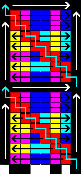
(a)

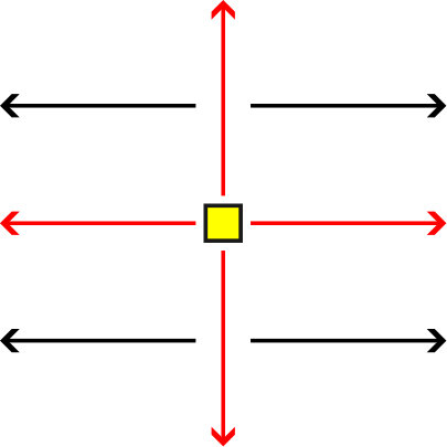
(b)

Figure 14: (a) The growth of the grid, forming pattern $p_{north}$, identical to pattern $p_{n}$, with adjustments made for expansion to the north, from its bottom-most row, which is the initial row on the plane $z=1$. The first tile placed in each row follows a diagonal path, colored in red for clarity, starting from the first tile to the right. Growth of each row expands left and right from the tile along the diagonal. Upon the leftmost and rightmost edges are bounding tiles, colored in black for clarity, which denote the leftmost and rightmost bounds of $p_{north}$. Once the diagonal makes contact with the left bound, it generates a top-bound at height $h+1$, where $h$ is the height at which the diagonal makes contact with the left bound. Once the top-bound’s signal is propagated to reach the right-bound, a new grid-forming diagonal is created, starting the process over again. (b) The infinite growth of $m\times m$ squares illustrated at a high level, with the initial $m\times m$ square which generates $p_{n}$ colored in yellow, direction of growth colored in red, and direction of copy assembly, which utilizes the signals of those assembled above or below them colored in black.

This basic assembly is used in all four cardinal directions in order to form a cross of $m\times m$ squares, each of which extends infinitely. Once a column is formed in either the east or west direction, and a corresponding row is formed in the north or south direction, tiles containing the bit values of that column to their north or south, and rows to their east or west are able to propagate out along those patterns created in the cross assembly. This allows for the infinite tiling of the same $m\times m$ square infinitely across the $\mathbb{Z}^{2}$ plane to form $p_{n_{\infty}}$.

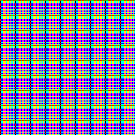
(a) Infinite tiling along the bit sequence $0110010010101$.

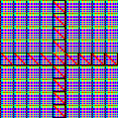
(b) Infinite tiling along the bit sequence $0110010010101$ with the cross assembly marked with red tiles along grid-creating diagonals, and black tiles along bounds.

Figure 15: Assemblies representing the infinite tiling of $m\times m$ squares corresponding to bit sequence $0110010010101$ across $\mathbb{Z}^{2}$. With creation and bounds marked, and unmarked.

7 Technical Details of the Construction for Theorem 6.1

In this section we include technical details of the construction used to prove Theorem 6.1. During the growth of the layer at $z=0$, the majority of the construction’s complexity lies in the simulation of Turing machine $M$ that simulates every aTAM system with $\leq n$ tile types. Here we provide details of the how $M$ accomplishes that.

We break the functionality of $M$ into pieces for which we define the pseudocode. The main function executed by $M$ is SimulateAllTileAssemblySystems, which takes the maximum number of tile types, $n$, in the systems to be simulated and can be seen in Algorithm 1. This function computes the number of systems to simulate, initializes the data structure used to contain the tile set definitions, then loops to simulate each system and retrieve the relevant bit value needed to construct pattern $p_{n}$.

Algorithm 1 An algorithm for simulating all aTAM systems with up to numTileTypes tile types of 8 colors, single-tile seeds, and at temperature 2 for a bounded amount of time. It returns a list of bits, one bit for each simulation.

1:procedure SimulateAllTileAssemblySystems(numTileTypes)

2:     $\texttt{P}=[]$ $\triangleright$ Initialize the pattern, which will be a list of bits

3:     $\texttt{numColors}=8$

4:     $\texttt{numGlues}=2*\texttt{numTileTypes}+1$ $\triangleright$ Maximum number of possible glues =

5:     $\triangleright$ numTileTypes glues of strength-1 +

6:     $\triangleright$ numTileTypes glues of strength-2 +

7:     $\triangleright$ the null glue

8:     $\texttt{numPossibleTileTypes}=\texttt{numColors}*\texttt{numGlues}^{4}$ $\triangleright$ Each tile can have one of

9:     $\triangleright$ numColors colors and 4

10:     $\triangleright$ glues (this will include ‘null’

11:     $\triangleright$ tile types with only null glues)

12:     $\texttt{numPossibleTileSets}=\texttt{numPossibleTileTypes}^{\texttt{numTileTypes}}$

13:     $\texttt{numSystems}=\texttt{numPossibleTileSets}*\texttt{numTileTypes}$ $\triangleright$ Make a system

14:     $\triangleright$ with each tile set and

15:     $\triangleright$ each tile type as seed

16:     currTileSet = InitializeTileSet(numTileTypes)

17:     for each $\texttt{i}\in[1,(\texttt{numPossibleTileSets}-1)]$ do

18:         for each $\texttt{tileType}\in\texttt{currTileSet}$ do $\triangleright$ Make a unique TAS with

19:              $\triangleright$ each tile type as the seed

20:              $\texttt{tas}=(\texttt{currTileSet},(\texttt{tileType},(0,0),2)$

21:              $\texttt{numSteps}=(2*\texttt{numSystems})^{2}$

22:              $\texttt{p}_{i}$ = SimulateTileAssemblySystem($\texttt{tas},\texttt{numSteps},\texttt{numSystems},\texttt{i}$)

23:              $\texttt{P}=\texttt{P}+\texttt{p}_{i}$

24:         end for each

25:         IncrementTileSet($\texttt{currTileSet},\texttt{numColors},\texttt{numGlues}$)

26:     end for each

27:     return P

28:end procedure

SimulateAllTileAssemblySystems utilizes a number of helper functions. The first is InitializeTileSet, which can be seen in Algorithm 2. It simply creates the data structure used to encode each tile of the tile set, starting each as the null tile.

Algorithm 2 A procedure to initialize the data structure representing a tile set.

1:procedure InitializeTileSet(numTileTypes)

2:     $\texttt{tileSet}=[]$ $\triangleright$ Start with an empty list

3:     for each $i\in[1,\texttt{numTileTypes}]$ do

4:         $\texttt{tile}_{i}=(0,0,0,0,0)$ $\triangleright$ Make the 5-tuple for a tile type

5:         $\triangleright$ (color, N glue, E glue, S glue, W glue)

6:         $\texttt{tileSet}=\texttt{tileSet}+\texttt{tile}_{i}$

7:     end for each

8:     return tileSet

9:end procedure

Next is the function used to increment to the next tile set to be simulated. Called IncrementTileSet, this can be seen in Algorithm 3.

Algorithm 3 Algorithm to increment the current tile set to the next possible tile set.

1:procedure IncrementTileSet($\texttt{currTileSet},\texttt{numColors},\texttt{numGlues}$)

2:     $\texttt{overflow}=\texttt{TRUE}$

3:     $\texttt{tileNum}=0$

4:     while $(\texttt{overflow}=\texttt{TRUE})$ and $(\texttt{tileNum}<len(\texttt{currTileSet}))$ do

5:         $\texttt{tile}=\texttt{currTileSet}[\texttt{tileNum}]$

6:         $\texttt{overflow}=\texttt{FALSE}$

7:         if $\texttt{tile}[0]==\texttt{numColors}$ then

8:              $\texttt{tile}[0]=1$

9:              $\texttt{overflow}==\texttt{TRUE}$

10:         else

11:              $\texttt{tile}[0]+=1$

12:         end if

13:         $\texttt{currLoc}=1$

14:         while $(\texttt{overflow}==\texttt{TRUE})$ and $(\texttt{currLoc}<5)$ do

15:              if $\texttt{tile}[\texttt{currLoc}]==\texttt{numGlues}$ then

16:                  $\texttt{tile}[\texttt{currLoc}]=1$

17:              else

18:                  $\texttt{tile}[\texttt{currLoc}]+=1$

19:                  $\texttt{overflow}=\texttt{FALSE}$

20:              end if

21:              $\texttt{currLoc}+=1$

22:         end while

23:         $\texttt{tileNum}+=1$

24:     end while

25:end procedure

The function SimulateTileSystem holds the logic for simulating each of the generated aTAM systems and also inspecting them to retrieve the necessary output bits. Its logic is shown in Algorithm 4, and a high-level overview of the data structures used to store the current tile set, assembly and frontier can be seen in Figure  16. SimulateTileSystem also has a few helper functions to be discussed below.

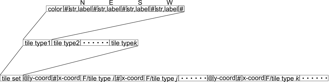
Figure 16: A high-level depiction of the encoding of the tile types, tile set, and assembly during a simulation. (Top) The encoding of a tile type consists of its color, followed by the definition of each side’s glue (i.e. its strength and label). (Middle) The encoding of a tile set consists of a list of each tile type’s definition. (Bottom) The encoding of a system being simulated consists of the definition of the tile set followed by a sub-list for each $y$-coordinate containing a tile or frontier location, where each such sub-list consists of a list of entries of the $x$-coordinates at that $y$-coordinate containing tiles or frontier locations. Each such location contains the encoding of the $x$-coordinate and either the definition of the type of the tile located there or, for a frontier location, the definitions of the glues that are adjacent to it (along with a special character to denote the location as a frontier location).

Algorithm 4 Algorithm to simulate a given aTAM system for a bounded amount of steps and return a pattern value.

1:procedure SimulateTileSystem($\texttt{tas},\texttt{numSteps},\texttt{pattSize},\texttt{index}$)

2:     $\texttt{tileSet}=\texttt{tas}[0]$

3:     $\texttt{seed}=\texttt{tas}[1]$

4:     $F=\{(0,0)\}$ $\triangleright$ Initialize the frontier

5:     $\alpha=\{\texttt{seed}\}$ $\triangleright$ Initialize assembly as seed

6:     UpdateFrontier($F,(0,0),\alpha,\texttt{tileSet}$)

7:     $s=0$

8:     while $s\leq\texttt{numSteps}$ do

9:         AddTile($F,\alpha,\texttt{tileSet}$)

10:         if $|F|=0$ then

11:              return $0$ $\triangleright$ System doesn’t make valid pattern

12:         else

13:              $s=s+1$

14:         end if

15:     end while

16:     $p=$GetPatternValue($\texttt{tileSet},\alpha,\texttt{pattSize},\texttt{index}$) $\triangleright$ Analyze pattern to

17:     $\triangleright$ find return value $p$

18:     return $p$

19:end procedure

The first helper function for SimulateTileSystem is UpdateFrontier, which can be seen in Algorithm 5 and is used to update the current set of frontier locations after a tile is added to an assembly by first removing the location of the newly added tile from the frontier, then checking all locations neighboring that newly added tile to see if they need to be added to the frontier.

Algorithm 5 A procedure that takes as arguments a set of frontier locations, one of the locations from that set, an assembly, and a tile set. It updates the frontier by adding any locations which neighbor the given location and have adjacent glues that would allow a tile of some type in the tile set to bind.

1:procedure UpdateFrontier($F,l,\alpha,T$)

2:     Remove location $l$ from $F$

3:     for $n\in\{(1,0),(-1,0),(0,1),(0,-1)\}$ do

4:         $l_{nbr}=l+n$

5:         $\texttt{glues}=[]$

6:         if $l_{nbr}\not\in\alpha$ and $l_{nbr}\not\in F$ then

7:              for $n_{2}\in\{(1,0),(-1,0),(0,1),(0,-1)\}$ do

8:                  $l_{nbr2}=l_{nbr}+n_{2}$

9:                  if $l_{nbr2}\in\alpha$ then

10:                       Let $t$ be the tile type at location $l_{nbr2}$ in $\alpha$

11:                       Let $g$ be the glue on the side of $t$ adjacent to $l_{nbr}$

12:                       $\texttt{glues}=\texttt{glues}+\texttt{g}$

13:                  end if

14:              end for

15:         end if

16:         if Sum of strengths of glues in $\texttt{glues}\geq 2$ then

17:              for $t\in T$ do

18:                  if Sum of strengths of glues of $t$ matching glues in $\texttt{glues}\geq 2$ then

19:                       $F=F\cup l_{nbr}$

20:                  end if

21:              end for

22:         end if

23:     end for

24:end procedure

The next helper function for SimulateTileSystem is AddTile, shown in Algorithm 6, the determines if and where a new tile can be added to an assembly, and adds one if possible.

Algorithm 6 A procedure that takes as arguments a set of frontier locations, an assembly, and a tile set, then places a fitting tile type into the first listed frontier location (if the frontier is not empty). It ensures the frontier and assembly are correctly updated to account for the added tile.

1:procedure AddTile($F,\alpha,T$)

2:     if $|F|=0$ then

3:         return $\triangleright$ Empty frontier, can’t add a tile

4:     else

5:         $f=F[0]$ $\triangleright$ Get the first location in the frontier

6:         for each $t\in T$ do

7:              if $t$ can bind in $f$ then

8:                  $\alpha=\alpha+(t,f)$ $\triangleright$ Add a tile of type $t$ in location $f$

9:                  $F=F-f$ $\triangleright$ Remove $f$ from the frontier

10:                  UpdateFrontier($F,f,\alpha,T$)

11:                  return

12:              end if

13:         end for each

14:     end if

15:end procedure

The function GetPatternValue inspects a given assembly to find the color of a tile at a location matching the current system’s index and, if found, returns a bit that will cause pattern $p_{n}$ to always have different colors at that index in the cells of the pattern. It simply returns 0 if the assembly fails to make a valid cell of a pattern.

Algorithm 7 Procedure for analyzing an assembly and finding the color of a tile at a given index in the pattern.

1:procedure GetPatternValue($\texttt{tileSet},\alpha,\texttt{pattSize},\texttt{index}$)

2:     Let $\texttt{BoundaryColors}=\{\texttt{Red},\texttt{Green},\texttt{Black},\texttt{White}\}$

3:     Let $\texttt{InteriorColors}=\{\texttt{Pink},\texttt{Blue}\,\texttt{Yellow},\texttt{Aqua}\}$

4:     $(\texttt{firstTileType},(\texttt{firstX},\texttt{firstY}))=\alpha[0]$ $\triangleright$ Get first tile in assembly list

5:     $\texttt{minX}=\texttt{firstX}$ $\triangleright$ Initialize min/max variables

6:     $\texttt{maxX}=\texttt{firstX}$

7:     $\texttt{minY}=\texttt{firstY}$

8:     $\texttt{maxY}=\texttt{firstY}$

9:     for each $\texttt{tile}\in\alpha$ do $\triangleright$ Find min/max coordinates of $\alpha$

10:         $\texttt{currX}=\texttt{tile}[1][0]$

11:         $\texttt{currY}=\texttt{tile}[1][1]$

12:         if $\texttt{currX}<\texttt{minX}$ then

13:              $\texttt{minX}=\texttt{currX}$

14:         end if

15:         if $\texttt{currX}>\texttt{maxX}$ then

16:              $\texttt{maxX}=\texttt{currX}$

17:         end if

18:         if $\texttt{currY}<\texttt{minY}$ then

19:              $\texttt{minY}=\texttt{currY}$

20:         end if

21:         if $\texttt{currY}>\texttt{maxY}$ then

22:              $\texttt{maxY}=\texttt{currY}$

23:         end if

24:     end for each

25:     if $\texttt{maxX}-\texttt{minX}\geq\texttt{pattSize}$ then $\triangleright$ $\alpha$ is wide enough to contain the pattern

26:         return InspectWidth($\alpha,\texttt{minX},\texttt{maxX},\texttt{index}$)

27:     else$\triangleright$ $\alpha$ must be tall enough to contain the pattern

28:         return InspectHeight($\alpha,\texttt{minY},\texttt{maxY},\texttt{index}$)

29:     end if

30:end procedure

The four helper functions for GetPatternValue are InspectWidth, InspectHeight, GetTileAtX and GetTileAtY, shown in Algorithms 8, 9, 10, and 11, respectively. The first two take as input an assembly and its greatest extent in the corresponding dimension, plus the index of the current simulation, and look for a tile with a boundary color, then a tile further along the corresponding dimension by index positions, and return a bit related to the color of the tile there. More specifically, based on the color of the tile found there, it will return a bit that will force $p_{n}$ to disagree on colors at all locations corresponding to that index value. (If a tile with a boundary color is not found, 0 is returned since the given assembly clearly cannot make pattern $p_{n}$.) GetTileAtX and GetTileAtY are simply used to find tiles at given coordinates in an assembly.

Algorithm 8 A procedure that takes an assembly, its horizontal bounds, and the index of the system being simulated, and searches horizontally to return a bit that ensures $p_{n}$ will have a different color at the index location than the assembly (or 0 if the assembly does not contain a valid pattern).

1:procedure InspectWidth($\alpha,\texttt{minX},\texttt{maxX},\texttt{index}$)

2:     $\texttt{currX}=\texttt{minX}$

3:     $\texttt{xTile}=$ GetTileAtX($\alpha,\texttt{currX}$)

4:     $\texttt{currColor}=\texttt{xTile}.\texttt{color}$

5:     while ($\texttt{currColor}\not\in\texttt{BoundaryColors}$) and ($\texttt{currX}<\texttt{maxX}$) do

6:         $\texttt{xTile}=$ GetTileAtX($\alpha,\texttt{currX}$)

7:         $\texttt{currColor}=\texttt{xTile}.\texttt{color}$

8:         $\texttt{currX}=\texttt{currX}+1$

9:     end while

10:     if $\texttt{currX}==\texttt{maxX}$ then

11:         return $0$ $\triangleright$ System failed to make valid pattern

12:     else

13:         $\texttt{indexTile}=$ GetTileAtX($\alpha,\texttt{currX}+\texttt{index}$)

14:         if $\texttt{indexTile}==\texttt{FALSE}$ then

15:              return $0$ $\triangleright$ System failed to make valid pattern

16:         else$\triangleright$ currColor is the color placed by this system at its unique index

17:              if $\texttt{index}==0$ then $\triangleright$ Boundary column

18:                  if $\texttt{currColor}\in\{\texttt{White},\texttt{Green}\}$ then $\triangleright$ Color of column value $1$

19:                       return $0$

20:                  else$\triangleright$ Color of column value $0$

21:                       return $1$

22:                  end if

23:              else

24:                  if $\texttt{currColor}\in\{\texttt{Aqua},\texttt{Blue}\}$ then $\triangleright$ Color of column value $1$

25:                       return $0$

26:                  else$\triangleright$ Color of column value $0$

27:                       return $1$

28:                  end if

29:              end if

30:         end if

31:     end if

32:end procedure

Algorithm 9 A procedure that takes an assembly, its vertical bounds, and the index of the system being simulated, and searches vertically to return a bit that ensures $p_{n}$ will have a different color at the index location than the assembly (or 0 if the assembly does not contain a valid pattern).

1:procedure InspectHeight($\alpha,\texttt{minY},\texttt{maxY},\texttt{index}$)

2:     $\texttt{currY}=\texttt{minY}$

3:     $\texttt{yTile}=$ GetTileAtY($\alpha,\texttt{currY}$)

4:     $\texttt{currColor}=\texttt{yTile}.\texttt{color}$

5:     while ($\texttt{currColor}\not\in\texttt{BoundaryColors}$) and ($\texttt{currY}<\texttt{maxY}$) do

6:         $\texttt{yTile}=$ GetTileAtY($\alpha,\texttt{currY}$)

7:         $\texttt{currColor}=\texttt{yTile}.\texttt{color}$

8:         $\texttt{currY}=\texttt{currY}+1$

9:     end while

10:     if $\texttt{currY}==\texttt{maxY}$ then

11:         return $0$ $\triangleright$ System failed to make valid pattern

12:     else

13:         $\texttt{indexTile}=$ GetTileAtY($\alpha,\texttt{currY}+\texttt{index}$)

14:         if $\texttt{indexTile}==\texttt{FALSE}$ then

15:              return $0$ $\triangleright$ System failed to make valid pattern

16:         else$\triangleright$ currColor is the color placed by this system at its unique index

17:              if $\texttt{index}==0$ then $\triangleright$ Boundary column

18:                  if $\texttt{currColor}\in\{\texttt{White},\texttt{Black}\}$ then $\triangleright$ Color of column value $1$

19:                       return $0$

20:                  else$\triangleright$ Color of column value $0$

21:                       return $1$

22:                  end if

23:              else

24:                  if $\texttt{currColor}\in\{\texttt{Aqua},\texttt{Yellow}\}$ then $\triangleright$ Color of column value $1$

25:                       return $0$

26:                  else$\triangleright$ Color of column value $0$

27:                       return $1$

28:                  end if

29:              end if

30:         end if

31:     end if

32:end procedure

Algorithm 10 A procedure that takes as arguments an assembly and $x$-coordinate value and returns a tile with that coordinate.

1:procedure GetTileAtX($\alpha,x$)

2:     for each $\texttt{tile}\in\alpha$ do

3:         $\texttt{currX}=\texttt{tile}[1][0]$

4:         if $\texttt{currX}=x$ then

5:              return tile

6:         end if

7:     end for each

8:     return FALSE

9:end procedure

Algorithm 11 A procedure that takes as arguments an assembly and $y$-coordinate value and returns a tile with that coordinate.

1:procedure GetTileAtY($\alpha,y$)

2:     for each $\texttt{tile}\in\alpha$ do

3:         $\texttt{currY}=\texttt{tile}[1][1]$

4:         if $\texttt{currY}=y$ then

5:              return tile

6:         end if

7:     end for each

8:     return FALSE

9:end procedure

7.1 Complexity analysis

Here we give a brief overview of the time complexity of Turing machine $M$ running on input $n$, which in turn determines the size of the $m\times m$ square formed for each pattern $p_{n}$.

As shown in Section 6.1, given a bound of $n$ tile types the number of aTAM systems simulated is $O(n^{4n^{4}+1})$, which we refer to at $T(n)$. Each of the $T(n)$ simulated systems is simulated for $O(T(n)^{2})$ steps.

A tile set of $n$ tile types requires $O(n\log{n})$ bits to represent. The assembly $\alpha_{i}$ of each simulated system $\mathcal{T}_{i}$ is represented as a combined list of assembly and frontier locations. (See Figure 16 for a high-level depiction.) This list will be separated into a sub-list for each $y$-coordinate that contains a tile and/or frontier location. The sub-list for each $y$-coordinate will consist of an entry for each $x$-coordinate such that the coordinate $(x,y)$ represents a location with a tile in $\alpha$ or is a frontier location. Each tile location contains a definition of the tile type located there, requiring $O(\log{n})$ bits, and each frontier location contains the definitions of any (up to a maximum of 4) glues that are adjacent to that location and their directions, also requiring $O(\log{n})$ bits. Without loss of generality, the seed tile is placed at $(0,0)$. Thus, the encoding of each $x$ or $y$ coordinate requires $O(\log{T(n)})$ bits, since the largest magnitude of any coordinate values can be $T(n)$ or $-T(n)$ if the simulation proceeds for $T(n)$ steps. This means that the encoding of each entry for an $x$-coordinate plus tile or frontier location requires $O(\log{T(n)}+\log{n})$ bits. Since $T(n)=O(n^{4n^{4}+1})$, $T(n)>>n$, so $O(\log{T(n)}+\log{n})=O(\log{T(n)})=O(n^{4})$.

There can be $O(T(n))$ tile and frontier entries representing an assembly, for a size of $O(n^{4}T(n))$. The addition of a tile and updating of the frontier requires $O(n^{4})$ traversals of the assembly, which is of size $O(n^{4}T(n))$, yielding a time per simulation step of $O(n^{4}T(n)n^{4})=O(n^{8}T(n))$. Each simulation proceeds for a maximum of $O(T(n)^{2})$ steps, yielding a simulation time of $O(n^{8}T(n)^{3})$. With a total of $T(n)$ simulations, the total run time if $O(n^{8}T(n)^{4})=O(n^{8}(n^{4n^{4}+1})^{4})$. Since the simulation of each step of $M$ requires 1 or 2 rows (depending on the direction that the head of $M$ must move and whether the next row of the simulation grows right-to-left or left-to-right), and each row increases in width by 1, this is the bound of both the height and width of the assembly once the module that simulates $M$ completes growth.

The final portion to grow in the $z=0$ plane is that which copies the pattern, which will be of length $T(n)$, across the entire width of the top row by increasing the width of the copied pattern by 3 for every 2 rows that grow upward, which themselves increase the width by 2. That means that approximately as many rows as the width of the top row before copying begins minus the width of the pattern are required, i.e., $O(n^{8}(n^{4n^{4}+1})^{4}-T(n))=O(n^{8}(n^{4n^{4}+1})^{4})$. Thus, this is the bound for the width and height of the assembly that grows in the plane $z=0$, making the $m\times m$ square for $m=O(n^{8}(n^{4n^{4}+1})^{4})$.

References

- [1] Adleman, L., Cheng, Q., Goel, A., Huang, M.D.: Running time and program size for self-assembled squares. In: Proceedings of the 33rd Annual ACM Symposium on Theory of Computing. pp. 740–748. Hersonissos, Greece (2001). https://doi.org/http://doi.acm.org/10.1145/380752.380881
- [2] Cannon, S., Demaine, E.D., Demaine, M.L., Eisenstat, S., Patitz, M.J., Schweller, R.T., Summers, S.M., Winslow, A.: Two hands are better than one (up to constant factors): Self-assembly in the 2HAM vs. aTAM. In: Portier, N., Wilke, T. (eds.) STACS. LIPIcs, vol. 20, pp. 172–184 (2013)
- [3] Doty, D., Fleming, H., Hader, D., Patitz, M.J., Vaughan, L.A.: Accelerating Self-Assembly of Crisscross Slat Systems. In: Chen, H.L., Evans, C.G. (eds.) 29th International Conference on DNA Computing and Molecular Programming (DNA 29). Leibniz International Proceedings in Informatics (LIPIcs), vol. 276, pp. 7:1–7:23. Schloss Dagstuhl – Leibniz-Zentrum für Informatik, Dagstuhl, Germany (2023). https://doi.org/10.4230/LIPIcs.DNA.29.7, https://drops.dagstuhl.de/entities/document/10.4230/LIPIcs.DNA.29.7
- [4] Drake, P., Patitz, M.J., Tracy, T.: Pattern self-assembly software (2024), http://self-assembly.net/wiki/index.php/Pattern_Self-Assembly
- [5] Evans, C.G.: Crystals that count! Physical principles and experimental investigations of DNA tile self-assembly. Ph.D. thesis, California Institute of Technology (2014)
- [6] Hader, D., Koch, A., Patitz, M.J., Sharp, M.: The impacts of dimensionality, diffusion, and directedness on intrinsic universality in the abstract tile assembly model. In: Chawla, S. (ed.) Proceedings of the 2020 ACM-SIAM Symposium on Discrete Algorithms, SODA 2020, Salt Lake City, UT, USA, January 5-8, 2020. pp. 2607–2624. SIAM (2020)
- [7] Hendricks, J., Patitz, M.J., Rogers, T.A.: Universal simulation of directed systems in the abstract tile assembly model requires undirectedness. In: Proceedings of the 57th Annual IEEE Symposium on Foundations of Computer Science (FOCS 2016), New Brunswick, New Jersey, USA October 9-11, 2016. pp. 800–809 (2016)
- [8] Lathrop, J.I., Lutz, J.H., Patitz, M.J., Summers, S.M.: Computability and complexity in self-assembly. Theory Comput. Syst. 48(3), 617–647 (2011)
- [9] Lathrop, J.I., Lutz, J.H., Summers, S.M.: Strict self-assembly of discrete Sierpinski triangles. Theoretical Computer Science 410, 384–405 (2009)
- [10] Patitz, M.J., Summers, S.M.: Self-assembly of decidable sets. Natural Computing 10(2), 853–877 (2011)
- [11] Rothemund, P.W.K.: Folding DNA to create nanoscale shapes and patterns. Nature 440(7082), 297–302 (March 2006). https://doi.org/10.1038/nature04586, http://dx.doi.org/10.1038/nature04586
- [12] Rothemund, P.W.K., Papadakis, N., Winfree, E.: Algorithmic self-assembly of DNA Sierpinski triangles. PLoS Biol 2(12), e424 (12 2004)
- [13] Rothemund, P.W.K., Winfree, E.: The program-size complexity of self-assembled squares (extended abstract). In: STOC ’00: Proceedings of the thirty-second annual ACM Symposium on Theory of Computing. pp. 459–468. ACM, Portland, Oregon, United States (2000)
- [14] Soloveichik, D., Winfree, E.: Complexity of self-assembled shapes. SIAM Journal on Computing 36(6), 1544–1569 (2007)
- [15] Tikhomirov, G., Petersen, P., Qian, L.: Fractal assembly of micrometre-scale DNA origami arrays with arbitrary patterns. Nature 552(7683), 67–71 (2017)
- [16] Winfree, E.: Algorithmic Self-Assembly of DNA. Ph.D. thesis, California Institute of Technology (June 1998)
- [17] Wintersinger, C.M., Minev, D., Ershova, A., Sasaki, H.M., Gowri, G., Berengut, J.F., Corea-Dilbert, F.E., Yin, P., Shih, W.M.: Multi-micron crisscross structures grown from dna-origami slats. Nature Nanotechnology pp. 1–9 (2022)
- [18] Woods, D., Doty, D., Myhrvold, C., Hui, J., Zhou, F., Yin, P., Winfree, E.: Diverse and robust molecular algorithms using reprogrammable dna self-assembly. Nature 567(7748), 366–372 (2019)