Towards Agile Robots: Intuitive Robot Position Speculation with Neural Networks

Abstract

The robot position speculation, which determines where the chassis should move, is one key step to control the mobile manipulators. The target position must ensure the feasibility of chassis movement and manipulability, which is guaranteed by randomized sampling and kinematic checking in traditional methods. Addressing the demands of agile robotics, this paper proposes a robot position speculation network(RPSN), a learning-based approach to enhance the agility of mobile manipulators. The RPSN incorporates a differentiable inverse kinematic algorithm and a neural network. Through end-to-end training, the RPSN can speculate positions with a high success rate. We apply the RPSN to mobile manipulators disassembling end-of-life electric vehicle batteries (EOL-EVBs). Extensive experiments on various simulated environments and physical mobile manipulators demonstrate that the probability of the initial position provided by RPSN being the ideal position is 96.67%. From the kinematic constraint perspective, it achieves 100% generation of the ideal position on average within 1.28 attempts. Much lower than that of random sampling, 31.04. Moreover, the proposed method demonstrates superior data efficiency over pure neural network approaches. The proposed RPSN enables the robot to quickly infer feasible target positions by intuition. This work moves towards building agile robots that can act swiftly like humans.

I Introduction

In recent years, mobile robotics has garnered significant attention within the realm of science and technology, undergoing rapid expansion. This surge in interest is attributed to its vast potential for applications, spanning diverse fields that include scientific experimentation, additive manufacturing, multi-robot cooperation, and collaborative efforts involving both robots and humans [1, 2, 3, 4]. As technology continues to advance, mobile robots have begun to exhibit more autonomy and intelligence, enabling them to perform tasks in a variety of complex environments [5]. This has ignited a compelling demand for profound research and innovation in the realm of Task and Motion Planning (TAMP) for mobile robots.

In the domain of task and motion planning for mobile robots, the definition of TAMP problems and the choice of planners with planning methodologies are significant. For different types of TAMP problems, different planners and planning methods can be selected to realize a variety of complex dynamic manipulation tasks [6, 7, 8, 9]. The search speed of TAMP problems can be greatly improved by designing guided planners that can be learned [10]. Additionally, the advances in artificial intelligence provide powerful solutions for particular tasks within mobile robotics, and the use of neural networks to learn the general of near-optimal heuristics can be used to design efficient neural planners [11, 12].

Figure 1: Example: TAMP framework of disassembling a screw on a distant EOL-EVB based on NeuroSymbolic AI. (Left) Task planning level. The planner outputs a sequence of action primitives to be executed according to the task. (Right) Motion planning level. Chassis position speculative results affecting the realization of the task.

Figure 2: Comparison of three chassis position sampling methods. (a) Randomized sampling motion planning (b) ANN method motion planning (c) Motion planning by using RPSN.

The emergence of third-generation artificial intelligence-Neurosymbolism [13, 14, 15, 16] provides a more effective solution to the TAMP problem, which is analogous to human subjective reasoning (subjective logic) through knowledge-driven logical systems, and to human subconscious perception (subconscious ”intuition”) through probabilistic learning of neural networks [17, 18]. This advances the current stage of AI systems from perceptual intelligence to cognitive intelligence. In our previous research, we built a NeuroSymbolic Task and Motion Planning Framework (NeuroSymbolic TAMP) based on Planning Domain Define Language (PDDL) [19, 20] to realize a robotic embodied control architecture [21, 22, 23, 24]. The framework uses PDDL to define disassembly primitives and introduces neural predicates to map sensor data to quasi-symbolic states for real-time computation, successfully accomplishing tasks such as continuous disassembly of end-of-life electric vehicle batteries (EOL-EVBs) screws. When it comes to manipulating the mobile robot for motion planning, the quality of the sampling of the target chassis position is directly linked to the robot’s task completion[25, 26, 27]. If the chassis position is too close to the working object, it may lead to collisions or robot kinematic singularities. Conversely, if the position is too far from the target, it can exceed the operational range of the robotic arm. When faced with a large workspace, multiple task types, and complex sequences of work to be performed, the accurate sampling of the chassis position of mobile robots is necessary.

In the motion planning task about the chassis, we need to know both the current chassis position and the intended target position for chassis motion in advance to complete the path planning and robot kinematics simulation. However, when dealing with a workpiece at a given location, the target chassis position is determined through random sampling [20]. This introduces uncertainty regarding whether the sampled position can effectively accomplish the task. So it is necessary to carry out the forward and inverse kinematics simulation of the robot in the simulator, which takes up a large amount of computational resources for simulation.

The inefficiency of randomly sampling and simulating, together with the gap between simulation results and the real situation, are the key bottlenecks preventing robots from moving towards agility. In the decision-making phase, motion control relies more on established logical measurements for targeted parameter resolution, rather than being able to swiftly adapt to dynamically changing physical environments. The concept of NeuroSymbolic AI introduces a novel approach that leverages the perceptual abilities of neural networks and integrates them with the differential problem-solving capabilities of physical simulators for motion scenarios. This fusion enables robots to enhance their adaptability, precision, and agility in every facet of motion planning. To achieve this, we introduce neural networks at the decision-making level. The work in this paper will demonstrate its validity.

This paper proposes a robot position speculation network(RPSN), a NeuroSymbolic AI based differentiable framework designed for motion planning of mobile robots. The RPSN offers a solution to the robot motion planning problem, eliminating the need for time-consuming and costly random sampling of target positions. When we tell RPSN the target pose of the part to be worked with, it can directly speculate a chassis target location with a high success rate for following steps, which is similar to the human mind. Moreover, the RPSN framework is data-efficient because differentiable IK imports human knowledge into the system. There are three main contributions that we have made:

1. We have programmed the robot’s forward and inverse kinematics in a differentiable manner within computational graphs for integration into the training process. This addresses challenges such as discontinuous functions to ensure gradient continuity.

2. We have introduced an innovative loss function designed to facilitate bootstrapping within the backpropagation process, even without ground truth inputs.

3. We have creatively utilized dropout to generate network randomization, which has yielded positive results.

II TAMP with RPSN

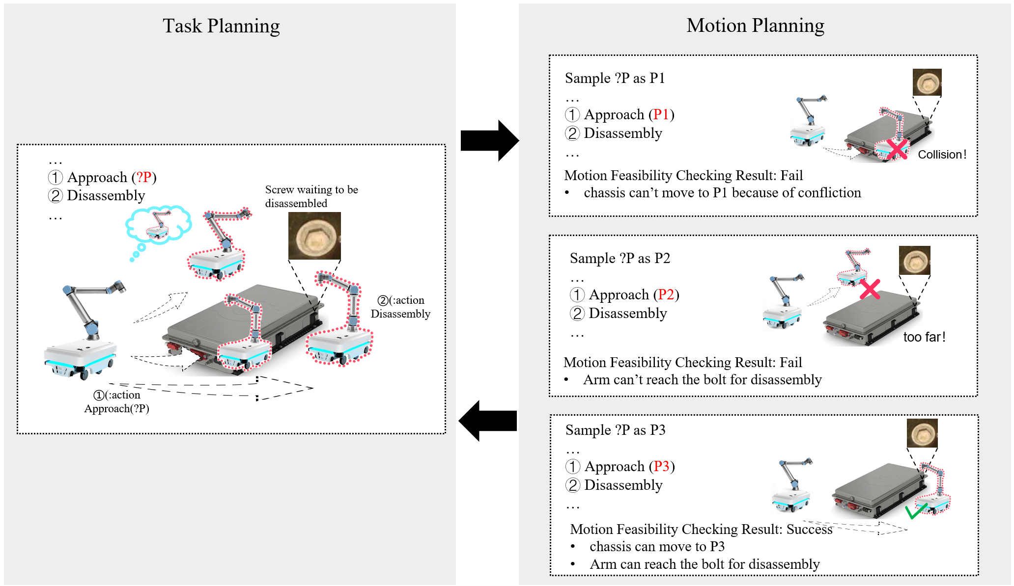
Figure 1 illustrates the whole process of TAMP based on neural symbolism and RPSN. Here, we present an example of a mobile robot disassembling a bolt from an EOL-EVB. The left side of Figure 1 is the task planning level, the system determines the current state that the robot is in based on the multimodal information such as torque, RGB images, depth images acquired by the multisensors, which is symbolically described using predefined neural predicates. Also, action primitives having preconditions and execution results are defined in the knowledge graph using the PDDL language. Once the target state is known, the system uses a logical search algorithm [23, 22] to find the best sequence of primitives to reach the final state from the current state. The right side of the image shows three distinct chassis target positions. Selecting an appropriate chassis position is extremely important because being too close can lead to collisions while being too far will exceed the robot’s workspace. The central concern in this task is how the mobile robot can efficiently and accurately perform robot position speculation to find the target location when the sequence is executed to move the mobile chassis position. In essence, when a mobile robot is required to perform a motion primitive, the challenge is to ensure that it reaches a viable position directly. This position should not only guarantee the object’s presence within the robot’s workspace but also assure the availability of a valid solution for the robot’s inverse kinematics at that specific position.

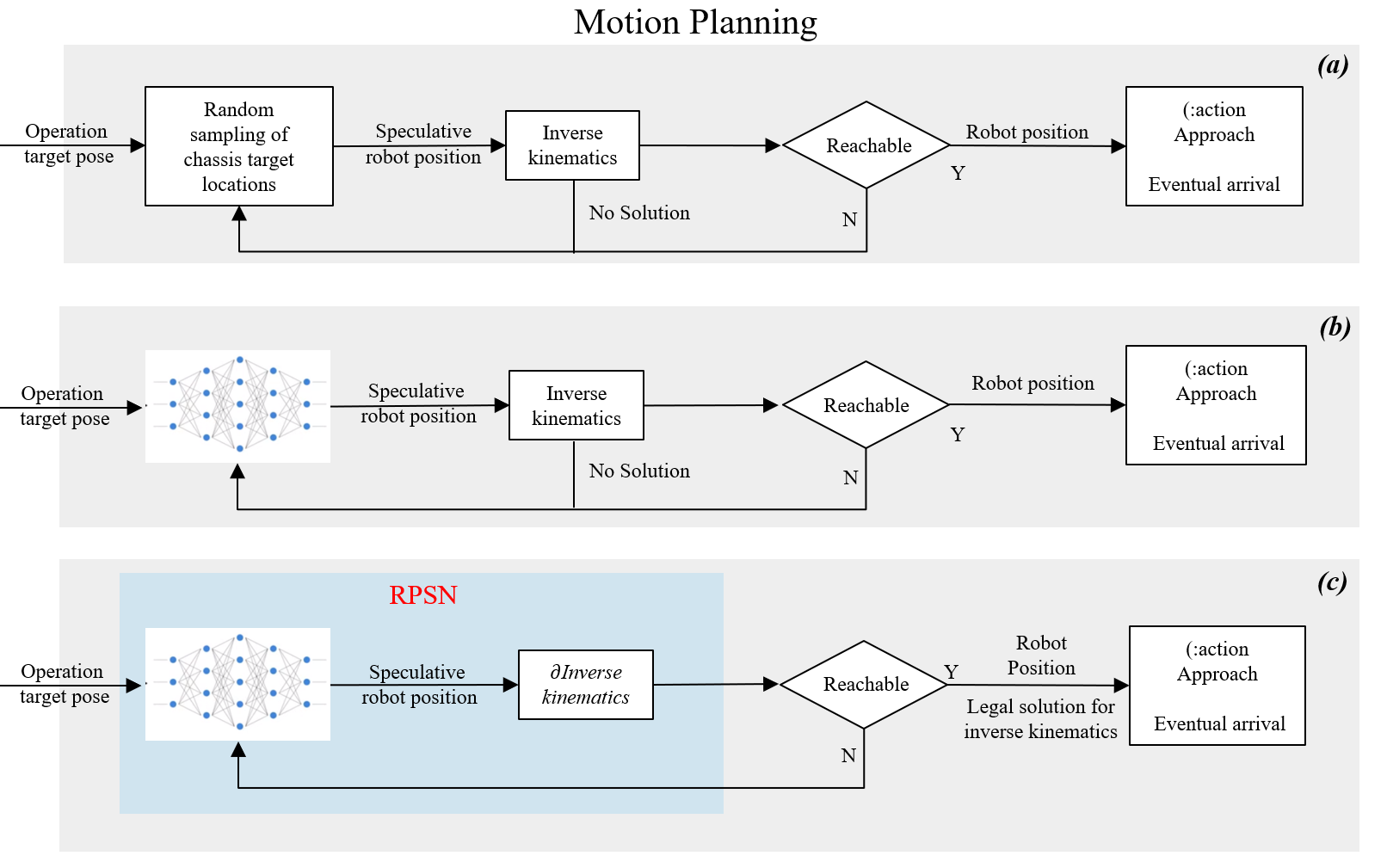
Figure 2 shows the differences and distinctions between motion planning using the traditional approach or using RPSN. Figure 2(a) is the common method of the PDDL-STREAM framework [20, 28]. For the chassis target position, the random sampling method presents an assumed chassis position, which is then employed in the robot’s inverse kinematics calculation to determine the feasibility of a valid solution and the robot’s reachability. However, Random sampling methods often necessitate closed-loop feedback and multiple sampling iterations to determine the correct final position. This prolonged process results in increased task duration and multiple recalculations for the robot’s navigation. With the help of neural networks (Figure 2(b)), this process can be optimized using a large amount of data training, through which we hope that the ANN can learn the implicit mapping relationship between the current position and the target position, thus outputting a more credible result. Compared with the previous two methods, the RPSN(Figure 2(c)) proposed in this paper consists of two modules: the Position Prediction Network and the Differentiable Kinematics Calculation Engine. When the pose of the bolt to be disassembled is inputted, the RPSN can directly output the position that the chassis should reach and provide the corresponding legal solutions for each joint, which is approximate to the subconscious intuition of human beings. This method will greatly improve the efficiency of motion planning. Figure 3 illustrates the specific end-to-end training and utilization. Comparative experiments on the three methods will follow in a subsequent section to showcase RPSN’s superiority in mobile robot motion planning.

It is worth emphasizing that the most essential difference between RPSN and traditional neural networks is that no ground truth data is provided during the training process. The forward and inverse kinematics algorithms are added to the training process of the neural network in a differentiable way and are involved in learning to steer the output values of the network before backpropagation. The traditional neural network computational graph will be greatly changed due to the addition of the robotic differentiable computation as a computational node after the forward propagation. The details of the algorithm’s differentiable process, the generalization method, and the guiding of the loss function will be elaborated in the next section.

Figure 3: RPSN training and working details. (Blue) PDDL neural predicates in task planning with action primitive execution. (Gray) Predicate Approach calling RPSN. (Yellow) RPSN training and loss function definition logic.

III RPSN Training Based on Differentiable Arithmetic Process Guidance

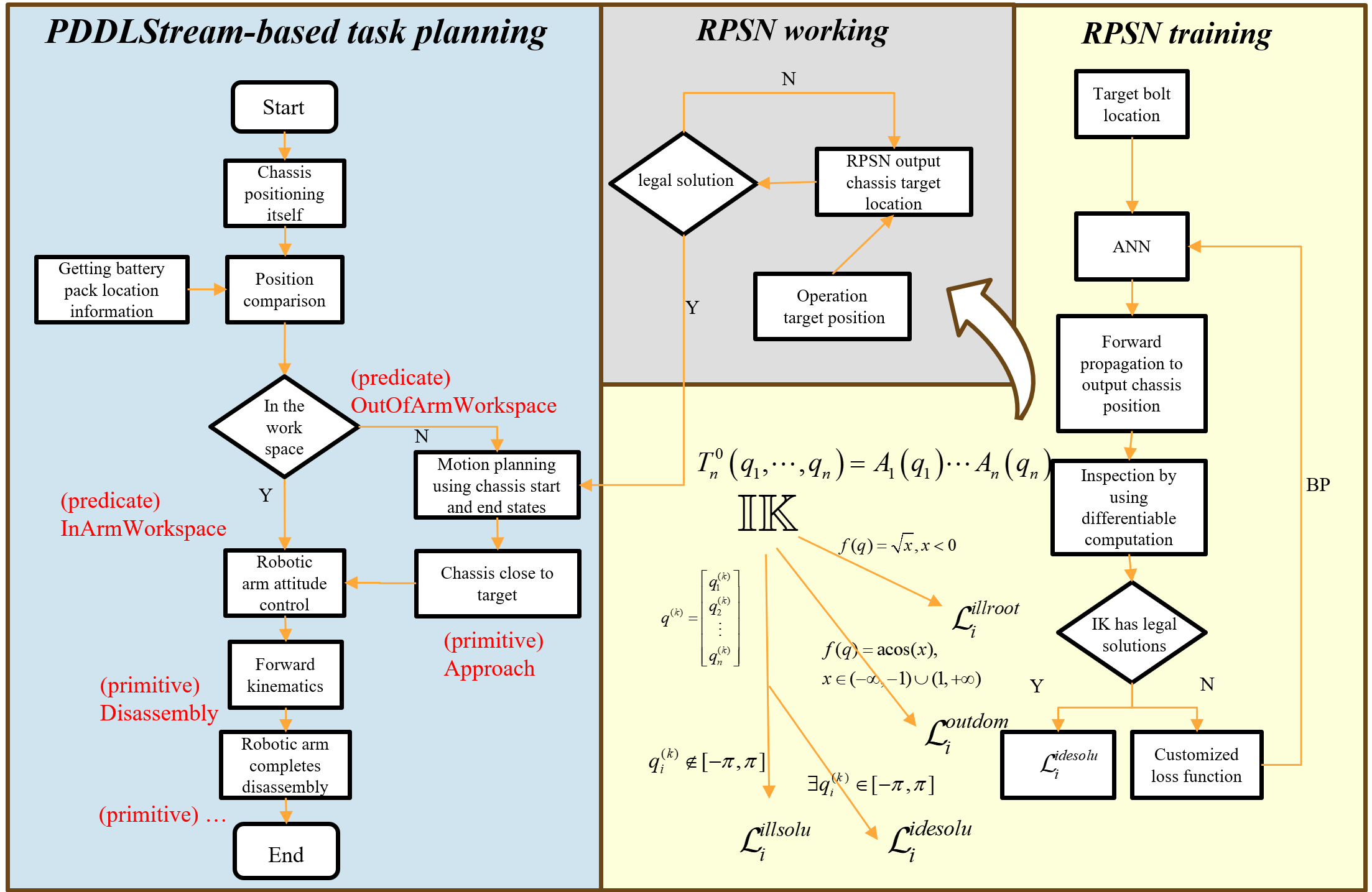
Figure 3 is a schematic diagram of the RPSN training process and working process. In the task planning stage, when a specific neural predicate triggers an action primitive that requires the robot to move, the pre-trained RPSN starts to work and provides the target position. The training stage of RPSN is particularly worthy of our attention, as it involves how to incorporate the differentiable programming property of a mature algorithm [29, 30, 31, 32] and incorporate it into the neural network training process. Its differentiable property approach should be generalizable to more mature algorithms with scalability and universality. This chapter will focus on the training process of RPSN and the general problems and solutions of differentiable programming.

III-A Computational graph construction and network training

The structure of the RPSN network requires that its robotic inverse kinematics computational engine must be written into the training process in a differentiable form. That means neither existing computational functions nor third-party libraries can be added as nodes to the computational graph of the neural network backpropagation due to their discontinuities. Before detailing the differentiation process, it is necessary to briefly describe the forward and inverse kinematics of the robot followed by the RPSN differentiable kinematics algorithm. In this paper, the differentiable algorithm follows the Denavit-Hartenbarg convention [33, 34], and the homogeneous transformation matrix of any joint $i$ concerning its predecessor joint $i-1$ can be expressed as:

$$H_{i}^{i-1}=A_{i}=Rot_{z,\theta_{i}}\operatorname{Trans}_{z,d_{i}}\operatorname{Trans}_{x,a_{i}}Rot_{x,\alpha_{i}}$$ (1)

Where $\theta$ is the joint angle, $d$ is the linkage offset, $a$ is the linkage length, and $\alpha$ is the linkage twist. When a total homogeneous transformation matrix $H_{total}$ is known :

$$H_{total}=\left[\begin{array}[]{cccc}n_{x}&o_{x}&a_{x}&p_{x}\\ n_{y}&o_{y}&a_{y}&p_{y}\\ n_{z}&o_{z}&a_{z}&p_{z}\\ 0&0&0&1\end{array}\right]=\left(\begin{array}[]{ll}R&d\\ 0&1\end{array}\right),$$ (2)

$$\quad R\in SO(3),\quad d\in\mathbb{R}^{3}$$

Then seek one or more solutions to the following equations, the inverse kinematics of the robot is formulated as:

$$\begin{gathered}T_{n}^{0}\left(q_{1},\cdots,q_{n}\right)=H_{total}\\ T_{n}^{0}\left(q_{1},\cdots,q_{n}\right)=A_{1}\left(q_{1}\right)\cdots A_{n}\left(q_{n}\right)\end{gathered}$$ (3)

The $q_{n}$ denotes the value of the nth joint, which is exactly the quantity we need to solve for in inverse kinematics. For the neural network input tensor, as in the previous example of the bolt pose to be disassembled, we give ${B}_{tar}=[\varphi,\theta,\psi,x,y,z],{B}_{tar}\in\mathbb{R}^{6}$. Considering that the robot’s actual working process is unchanged compared to the chassis position, so its pitch angle, lateral inclination, and longitudinal displacement should be Zero. Under the action of the Position Prediction Network, the robot target chassis position ${B}_{rob}=[\psi,x,y]$ is obtained, with its positive kinematics formulae derived from Eq. 1 for a six-axis robotic arm as:

$$H_{total}=\prod_{i=0}^{5}H_{i}^{i+1}$$ (4)

Then the solution of its inverse kinematics under the differentiable $\mathbb{IK}$ computational engine proposed in this paper can be expressed as:

$$\left\{\begin{matrix}solu_{angle}=\mathbb{IK}(H_{total})=\mathbb{IK}(H_{rob}^{Transpose}\cdot H_{tar})\\ H_{rob},H_{tar}=\mathbb{S}(B_{rob},B_{tar})\end{matrix}\right.$$ (5)

$$solu_{angle}\in\mathbb{R}^{8×6}$$

where $\mathbb{S}$ is the differentiable transformation engine. $\mathbb{S}$ represents the procedure of transforming the neural network’s output sequentially into Eulerian coordinates, followed by conversion into a rotation matrix, and ultimately into a homogeneous transformation matrix. These successive transformations are essential preparations for the $\mathbb{IK}$ process and hold the crucial property of being fully differentiable. The $\mathbb{IK}$ is a differentiable computational engine for the inverse kinematics algorithm. The inverse kinematics solves eight sets of solutions, each with six joint values, corresponding to the six joints of the six-axis robotic arm, which can be expressed as:

$$\text{For }k=1,2,\ldots,8\text{ and }n=1,2,\ldots,6$$ (6)

$$q^{(k)}=\begin{bmatrix}q_{n}^{(k)}\\ q_{n}^{(k)}\\ \vdots\\ q_{n}^{(k)}\end{bmatrix},\quad\text{where}\quad q_{n}^{(k)}\in[-\pi,\pi]$$

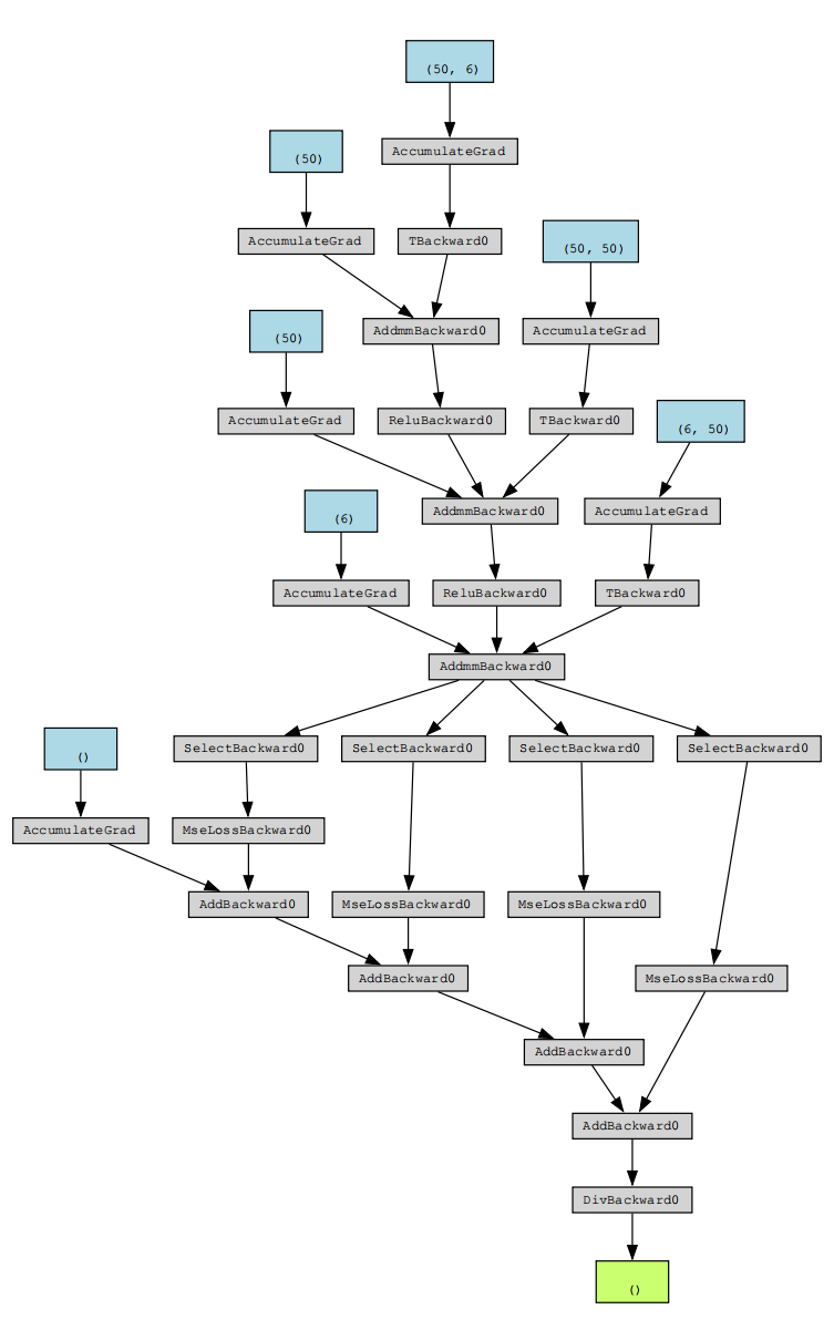
During programming, in order to make this solution process differentiable, we redefine the traditional matrixed inverse kinematics solution by defining differentiable computational processes such as $\mathbb{IK}$ and $\mathbb{S}$ using tensor operations to discretize the angular solution. This ensures that the robot’s inverse kinematics solution can be added to the computational graph. In particular, it is important to note that the Pytorch framework already provides some computational methods that can be used in writing algorithms. Including but not limited to torch.mm matrix product, torch.stack dimensional reorganization, and so on, which must be differentiable to be added to the computational graph as part of the generalized forward propagation. However, in the process of differentiable computation for traditional computational methods, there are still some non-differentiable functions or computations. The solutions to these problems will be detailed in the next section. When we add differentiable computational processes such as $\mathbb{IK}$ and $\mathbb{S}$ to the computational graph, the computational graph becomes extremely complex. Figure 4 shows the computational graph under the ANN method. Blue nodes symbolize the leaf nodes, while gray nodes signify intermediate nodes responsible for computational operations. Notably, the MSE loss function (’MseLossBackward0’ in the figure) actively participates in the forward propagation process. As a comparison, the computational graph of the real participation in RPSN is too complex to be presented intuitively. Please download and check it at the link (see https://sites.google.com/view/sjtu-rpsn). Each node in the computational graph is a differentiable mathematical operation, and we must ensure that each step of the computation is differentiable thereby ensuring that the computational graph is passable. In that case, forward propagation can take place, and special loss definitions are performed after passing through the differentiable computational engine to guide the learning of the network.

Figure 4: Computational graph of MLP with MSE

III-B Details of the differentiable methodology

In the process of differentiating the entire computation, we present the following three difficult problems:

1. Not all parts of forward and inverse kinematics can be easily differentiated; How can discontinuous functions or functions beyond the domain of definition be differentiable and participate in the computational graph?

2. RPSN as a model without ground truth data involved in training, how can the loss function be defined to have an effective bootstrap for training?

3. The parameters of the differentiable network are fixed after the training is completed, how to ensure its feedback process as well as the randomness of the network if it fails to give a legitimate solution during prediction?

For the first question, we will illustrate the general methodology with examples of the atan2 function and the $arccos$ function that jumps out of the domain of definition during the training of the RPSN. For the second question, we will present the loss functions defined by the results triggered by the different scenarios during the computation of $\mathbb{IK}$, as shown in detail in Figure 3.

The tangent function has a period of 180 degrees. When calculating the arctan function, there can be multiple tangent values for a given angle. The standard Math.atan function provides a single angle value, making angle determination complex, and it results in infinite values at 90 degrees and 270 degrees of tangent. In robot inverse kinematics, we employ the atan2 function as an effective solution for the inverse tangent. The atan2 function is defined as follows:

$$\text{atan2}(y,x)=\begin{cases}\arctan\left(\frac{y}{x}\right)&\text{if }x>0\\ \arctan\left(\frac{y}{x}\right)+\pi&\text{if }x<0\text{ and }y\geq 0\\ \arctan\left(\frac{y}{x}\right)-\pi&\text{if }x<0\text{ and }y<0\\ \frac{\pi}{2}&\text{if }x=0\text{ and }y>0\\ -\frac{\pi}{2}&\text{if }x=0\text{ and }y<0\\ \text{undefined}&\text{if }x=0\text{ and }y=0\end{cases}$$ (7)

It is clear that such an atan2 function is intermittent and its participation in the computational graph leads to a direct break in the gradient. Therefore it is necessary to redefine the forward and backward propagation process of the function itself as shown in Algorithm 1.

Algorithm 1 Differentiable Four-Quadrant Arctangent

1:class Atan2Function:

2:$\triangleright$ From torch. autograd.Function   

3:function forward($y,x$)

4:     $result\leftarrow$ calculate_atan2($y,x$)

5:$\triangleright$ calculated using the discrete atan2 function

6:     $ctx\leftarrow$save_for_backward($x,y$)

7:     return tensor($result,\text{requires\_grad}=\text{True}$)

8:$\triangleright$ ctx records the return of the results   

9:end function  

10:function backward($\text{ctx},\text{grad\_output}$)

11:      $x,y\leftarrow$ saved_tensors(ctx)

12:      $grad\_y\leftarrow$$\frac{\mathrm{d}}{\mathrm{d}y}\text{atan2}(y,x)\leftarrow x/(x^{2}+y^{2})$

13:      $grad\_x\leftarrow$$\frac{\mathrm{d}}{\mathrm{d}x}\text{atan2}(y,x)\leftarrow-y/(x^{2}+y^{2})$

14:      return $\text{grad\_output}\times grad\_y,\text{grad\_output}\times grad\_x$   

15:end function

16:function main

17:      $y\leftarrow$ get_input_y

18:      $x\leftarrow$ get_input_x

19:      $atan2\leftarrow$ Atan2Function.apply($y,x$)

20:end function

Atan2Function defines its propagation process in the form of a class. While forward propagation computes the results and stores the values of the nodes, the derivation of backpropagation can be expressed as the gradient of the node equals the result of multiplying the partial derivatives of that node by the cumulative gradient passed from the previous node. The relationship can also be seen as a concrete application of the chain rule. In this way, this inherently non-differentiable function successfully participates in the computational graph. It turns out that by simply changing the function’s body, this approach can be applied to address a range of formally discontinuous functions, ensuring computational differentiability. This will be a valuable asset in our differentiable programming workflow. Another frequent differentiable error in inverse kinematics occurs when an intermediate variable falls outside the domain of the mathematical function that operates on it. When confronted with this problem, our core idea is to continue to use the pattern of Algorithm 1 to change the forward and inverse operations of the function. Taking the most common $arccos$ function as an example, we know that:

$$F(x)=0\leq\cos^{-1}(x)\leq\pi,\text{where}-1\leq x\leq 1$$ (8)

When it appears that the value of the previous node in the computational graph is outside its domain of definition, we construct a new customized extended differentiable function $G(x)$, with the core arithmetic function $arccos$ of the current node as a base function. Taking $\delta>0$ and $\delta$ as sufficiently small:

$$G(x)=\begin{cases}-\frac{(x-(-1+\delta))}{\sqrt{1-(-1+\delta)^{2}}}+\cos^{-1}(-1+\delta),\text{if }x\leq-1+\delta,\\ \cos^{-1}(x),\hskip 51.21504pt\text{if }-1+\delta<x<1-\delta,\\ -\frac{(x-(1-\delta))}{\sqrt{1-(1-\delta)^{2}}}+\cos^{-1}(1-\delta),\text{if }x\geq 1-\delta.\end{cases}$$ (9)

In our formula, we employ the concept of tangent lines for construction. This is done because, inside the domain of the definition of the $arccos$ function, we want it to be computed normally and participate in defining the loss function. At the same time, the unsatisfactory part outside the domain of definition can have such a large slope that it is penalized by the network preference without interrupting the computation of the graph. To do this, we need to ensure that the newly constructed functions have equal values of the first-order derivatives at the discontinuity points.

This ensures that even if the value passed in from the previous node is out of the definition domain, the whole computation engine will not be terminated due to error reporting. In practice, this change not only ensures the program’s normal execution but also allows us to incorporate the out-of-definition domain into the loss composition. This is beneficial because this region typically has a steeper slope, resulting in a larger contribution. During backpropagation, the out-of-definition domain is penalized preferentially, represented as $L^{outdom}_{i}$ in Figure 3.

The solution to the second difficulty is inspired by the fact that when the input does not give a ground truth, the only pointers to training come from the various types of anomalies and their defined losses during the computation. If we can incorporate these losses into the bootstrapping of the neural network, the neural network will output outputs that can pass through all the computational maps to ultimately produce a legitimate solution. Naturally, this is a qualitative analysis, while the quantitative calculation of RPSN losses is provided by the following equation:

$$\mathcal{L}^{total}=\frac{1}{N}\sum_{i=1}^{N}( \mathbb{U}\cdot\delta_{illroot}\mathcal{L}^{illroot}_{i}+\mathbb{U}\cdot\delta_{outdom}\mathcal{L}^{outdom}_{i}$$ (10)

$$+ \delta_{illroot}\mathcal{L}^{illsolu}_{i}+\delta_{idesolu}\mathcal{L}^{idesolu}_{i})$$

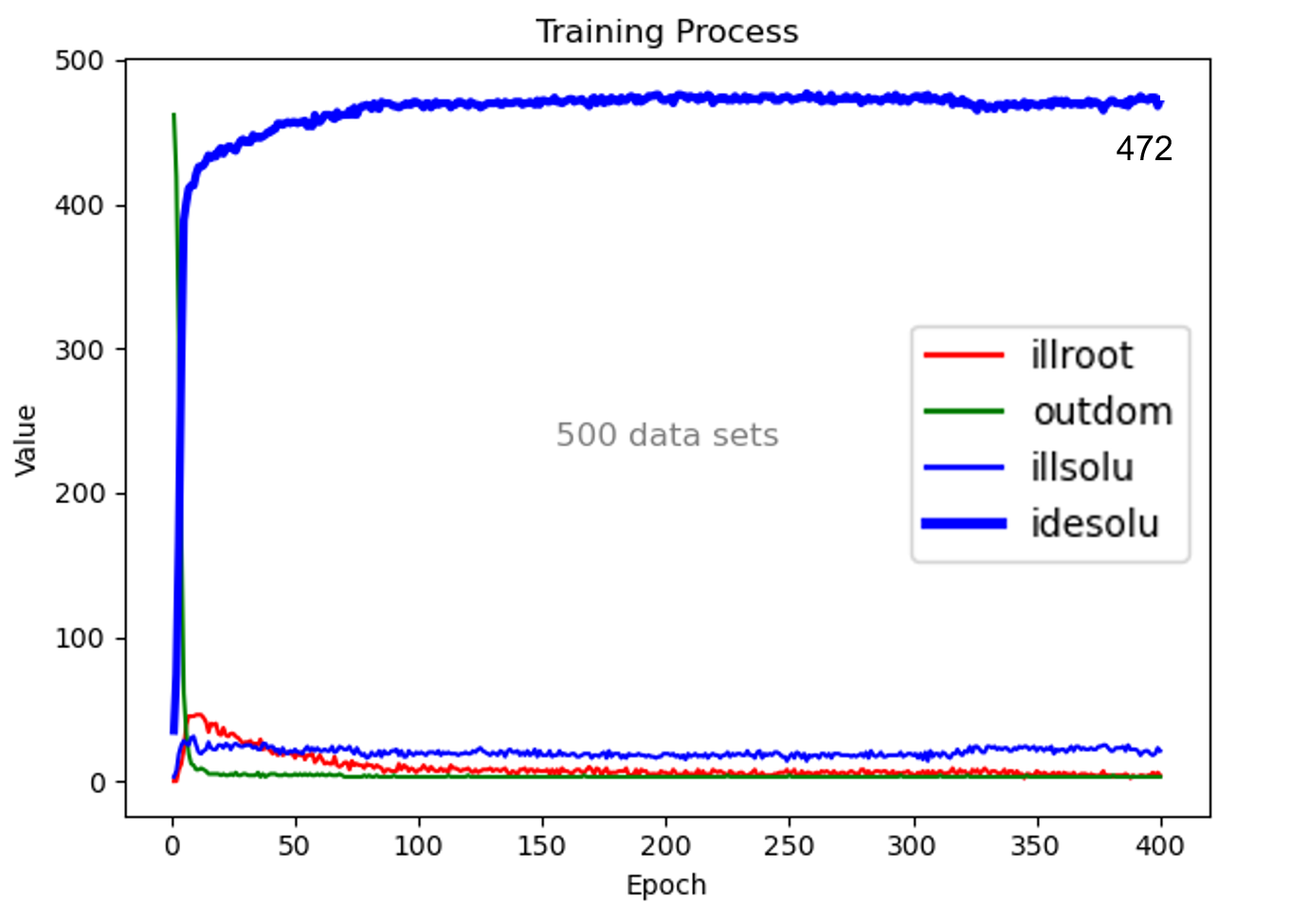
Where $\mathcal{L}^{illroot}_{i}$ as well as $\mathcal{L}^{outdom}_{i}$ denote exactly the penalties for the location prediction network data on the wrong branch during the differentiable computation process. They guarantee that the inverse operation has the result as shown in Eq. 6, even if the solved angle value is illegal. For numerically illegal angle values beyond $[-\pi,\pi]$, we use $\mathcal{L}^{illsolu}_{i}$ to penalize them. Obviously, if there exists any one of the eight sets of solutions where all the angular values of the angular solutions are within the legal range, the loss will be defined as 0, that is, $\mathcal{L}^{idesolu}_{i}$. The $\delta$ in Eq. 10 represents the weighting relationship between the different parts of the losses, which will determine which losses are preferentially penalized during backpropagation. In particular, for the inverse kinematics computation process included in the RPSN, we specifically define $\mathbb{U}$. When it takes 1, the loss function takes into account the loss from all the errors in the inverse kinematics computation process that deviates from the correct data flow, which is the task-specific loss. When it takes 0, we only define the loss and guide the training for one or more sets of illegal values in the final angular solution. Apparently, the former is more relevant for the present application scenario and the loss is defined more strictly, while the latter is an attempt of ours regarding the definition of loss in general problems and generalized scenarios.

To address the third challenge, we introduced an additional Dropout layer to the Position Prediction Network of RPSN, as illustrated in Table I. During testing, the Dropout layer remains active. When the Differentiable Kinematics Calculation Engine detects unsatisfactory outputs from the trained model, the testing process is restarted, and RPSN generates a fresh set of solutions. Since no loss is computed and no backpropagation is performed during this phase, the Dropout layer plays a crucial role in introducing randomness. Each regenerated result is generated by accessing the well-trained model, and any prior failures do not influence the current outcome.

IV Experiments and Results

IV-A Experiments Setup

Figure 5: Hardware platform

Figure 6: Training plots for the three methods. Top-down training accuracy curves for ANN, RPSN1, and RPSN2 respectively (with 500 sets of data for example).

Figure 7: Test accuracy curves for the three methods after training with different data amounts. The data volume ranges from 50 to 3200 groups.

In order to validate the effectiveness of the proposed method in this work, we use the disassembly of EOL-EVBs bolts as a practical application scenario to explore the performance demonstrated by the RPSN in terms of training and testing.

TABLE I: Training information for each model

Model	Composition	Loss function	Hyperparameter optimization
ANN	input_layer = 6 hidden_layer = 50 Dropout hidden_layer = 50 output_layer = 6	MSE	Ray.tune
RPSN1	input_layer = 6 hidden_layer = 50 Dropout hidden_layer = 50 output_layer = 3 $\mathbb{IK}$	$L^{total}$ $\mathbb{U}=1$	Ray.tune
RPSN2	input_layer = 6 hidden_layer = 50 Dropout hidden_layer = 50 output_layer = 3 $\mathbb{IK}$	$L^{total}$ $\mathbb{U}=0$	Ray.tune

TABLE II: Training Configure

Configure	Information
CPU/GPU	Intel Core i7-12700H/RTX 3060
Epoch	400
Learning rate	uniform(0.001, 0.01)
Batch size	choice([2,4,5,8,16])
Scheduler	ASHAScheduler
Grace period	150

TABLE III: Experimental Setup Introducing Randomness

	Dropout(Training)	Dropout (Testing)	Epoches	Dropout Rate
Case1	Deactivated	Deactivated	400	None
Case2	Activated	Activated	1000	2%-15%(use Ray-tune)
Case3	Deactivated	Activated	400	Consistent with case2 optimal result

Figure 8: Real-world experiments information and results.

Figure 9: The effect of randomization on the convergence of the training process.

TABLE IV: Average sampling times for each model

	Average samples(times)
Random sampling	31.04
Pure ANN	3.06
RPSN1	1.28
RPSN2	1.42

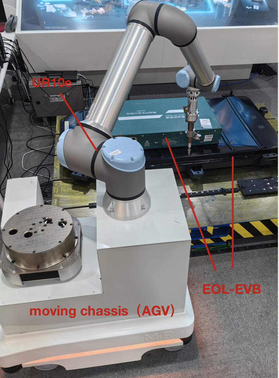
Figure 5 is our experimental hardware platform, which consists of an AGV trolley with its mounted 6-axis collaborative robot UR10e working on a to-be-disassembled EOL-EVB.

As Figure 2 introduces the RPSN structure, its Position Prediction Network is a common ANN model. Therefore, we conducted comparative experiments to demonstrate the difference in training outcomes when incorporating the computational engine for differentiable kinematics into the computational graph compared to a single ANN. The specific experimental training information is shown in Table I. We built the network model based on PyTorch and provided the training of ANN with the end-effector position required for the disassembly task in the same coordinate system with a chassis position that can accomplish the disassembly task. The loss between the network output and the ground truth is defined by MSEloss. For the training of the RPSN, the input data is a single end-effector pose required for the disassembly task, and its loss can be categorized into two cases according to the definition of Eq. 10. RPSN1 represents a more stringent task-specific loss, while RPSN2 represents a more general loss based on the use of a differentiable method as described in the previous section. In this case, the output dimension of the ANN is kept the same as the input data, making it easy to learn the mapping relationship between the spatial computational transformations during the training process.

To evaluate model performance under varying data volumes effectively, we designed ten different data volume sets, ranging from a minimum of 20 groups to a maximum of 3200 groups, for training and testing the three models. To ensure that the training hyperparameters are optimal under different data volumes and model conditions, we use Ray-tune [35] to search for optimal hyperparameters. It is guaranteed that each network model is randomly selected at least 30 times for hyperparameters under each data volume, and the network models trained with optimal hyperparameters are recorded with their test results. Training-related information is shown in Table II.

IV-B Experiments Details

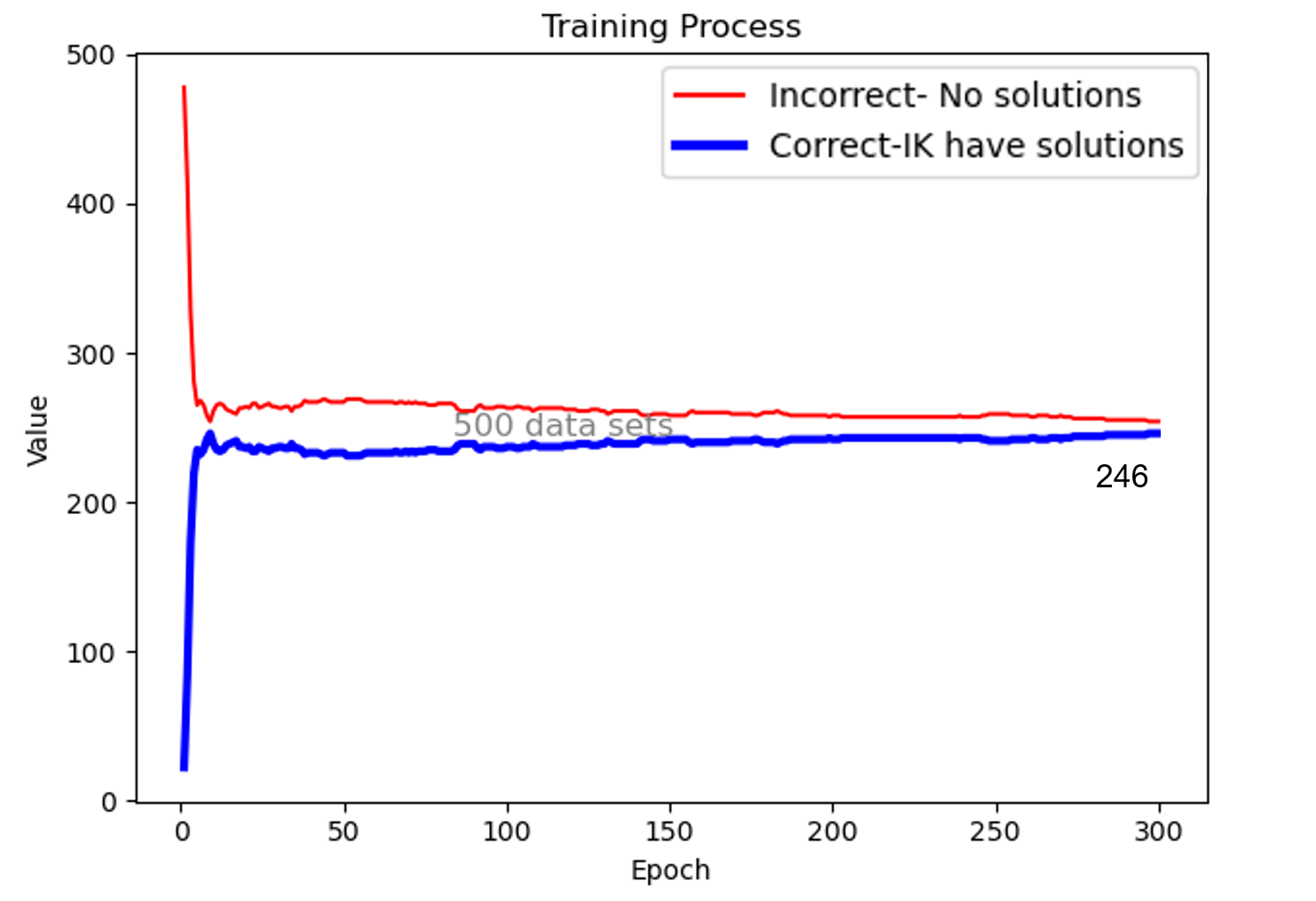
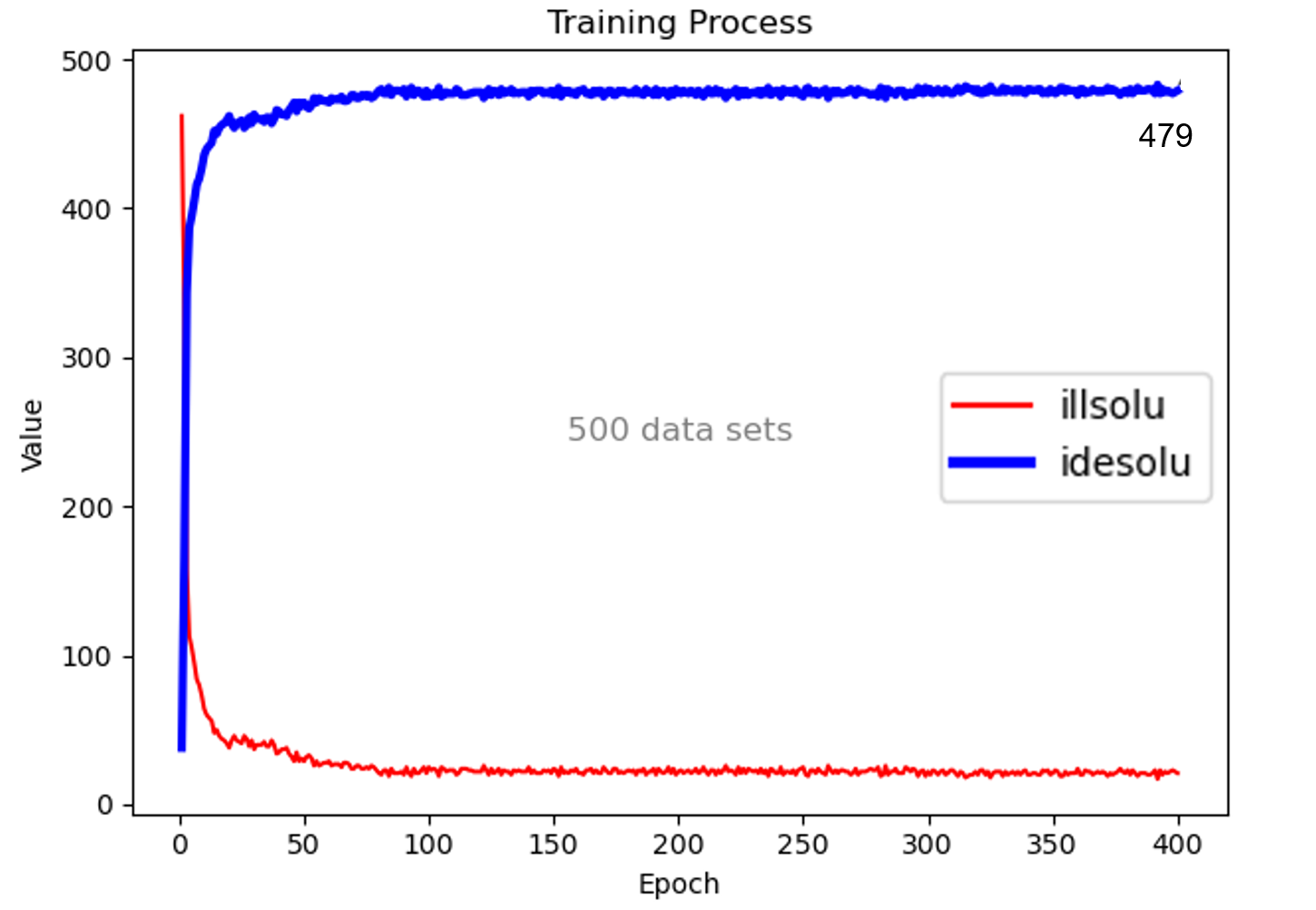
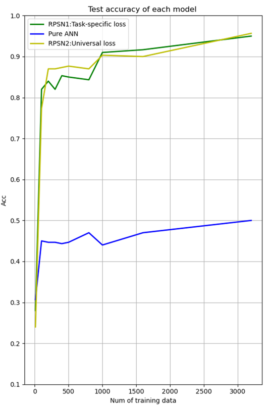
Due to the large number of experimental batches, we chose the training process of the three models in 500 sets as shown in Figure 6. Compared to the RPSN, the ANN network converges faster and has largely converged before 50 epochs. However, the large computational graph does not make the training process slow and time-consuming for the RPSN, which basically reaches convergence around 100 epochs and has a slow increase thereafter. The vertical coordinate represents the amount of data passed along with the training. The final training accuracy of the ANN method converges at around 53.69%, while the RPSN is higher than 94% for both cases. Figure 7 displays the test set results obtained from training three different models with varying amounts of data, with the RPSN model achieving the highest test accuracy at 95.67%. Meanwhile, ANN needs larger data support in training its parameters in a more optimal direction. The existing volume of data falls short of meeting the parameter refinement requirements for ANN, resulting in a test accuracy of approximately 50%. In contrast, the RPSN demonstrates an impressive accuracy exceeding 90% with only 1000 sets of training data. This excellent data efficiency can be attributed to the inclusion of differentiated kinematics algorithms as a priori knowledge within the framework.

It is important to emphasize that the experimental results depicted in Figures 6 and 7 represent explorations into the fundamental performance of RPSN, undertaken without the introduction of randomization. Compared to random sampling methods, RPSN shows amazing advantages in small data size, no ground truth, and fewer epochs of the training process. However, when undesirable situations below 5% occur, the fixed model requires multiple network models that have completed training to work together to ensure a 100% task completion rate. Thus, we introduce the network randomization methods described in Section III-B for a more in-depth comparative experimental exploration by controlling the degree of randomization during network training and testing. In this way, we aim to achieve a 100% success rate by relying solely on the combination of a single pre-trained RPSN with the feedback mechanism.

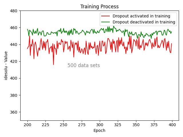
Table III shows the comparison experiments conducted with RPSN1 as the base network. In Case 1, the dropout layer is deactivated during both the training and testing phases, while the number of neurons in the hidden layer remains constant throughout the operation of RPSN. The experimental results are shown in Figures 6 and 7. Case 2 is the usage of dropout involved in training and testing as mentioned in Section III-B, and randomization occurs not only in the training process but also in the prediction process. Case 3 is based on the training of case 1, where network randomization is activated only in the testing phase. The selection of 1000 training epochs in Case 2 is deliberate. We have illustrated the training details for epochs 200-400, as depicted in the figure 9. The only variable considered was the introduction of randomization. When randomization is introduced into the training process of RPSN, the number of legal solution sets still exhibits significant fluctuations around the 400th epoch, showing an overall upward trend. Clearly, more training is required to achieve a better convergence effect. Figure 10 shows the performances of the three methods with different datasets.

Figure 10: Comparative experiments on RPSN with the introduction of randomization methods.

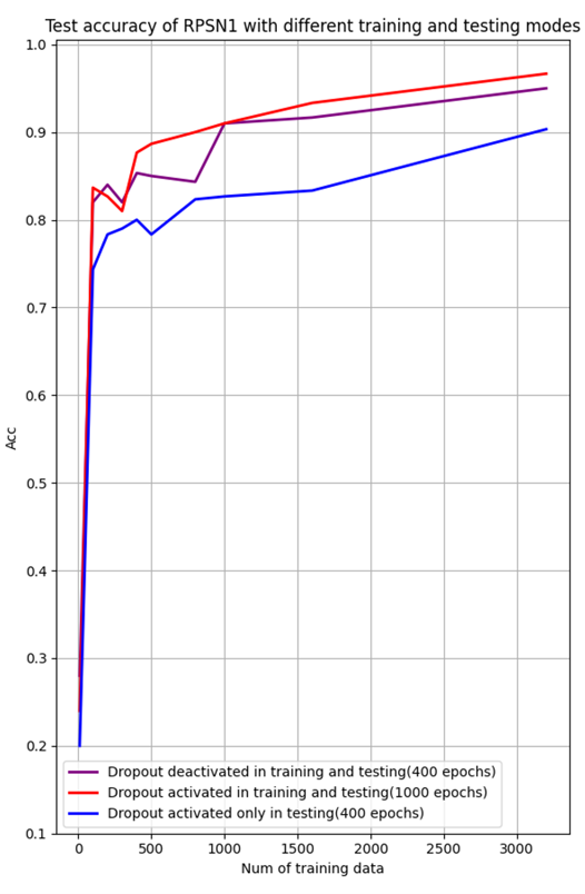
Through experiments, it is found that when the randomization method is introduced into the training and testing process, the accuracy has more obvious fluctuations in adjacent epochs. The reason for this is that the dropout’s culling of hidden neurons is completely randomized, which prevents the network from overly relying on certain neurons to get the desired output. Therefore, when randomization is involved in training, the RPSN needs to go through more rounds to achieve a similar accuracy as in case 1, and the introduction of randomization makes the individual hidden neurons more homogeneous. The experimental results show that after introducing the randomization method proposed in this paper, the RPSN achieves a single prediction accuracy of 96.67%, but it takes longer time and training epochs to reach convergence. The accuracy of this method is significantly higher than that of the method in case 3 where randomization is introduced only in testing. Therefore, despite the fact that the addition of randomization increases the training epoch, we still prefer this approach in our deployments

To further validate the advantages of RPSN, we provide the same to-be-disassembled bolt pose for different motion planning methods. The aim is to determine how many times of samples are required to reach the final chassis position when using various methods. The experimental results are shown in Table IV, where we provided 300 sets of data and calculated the mean value of the number of times all data were sampled.

IV-C Real Device Experiments in Disassembly Scenarios

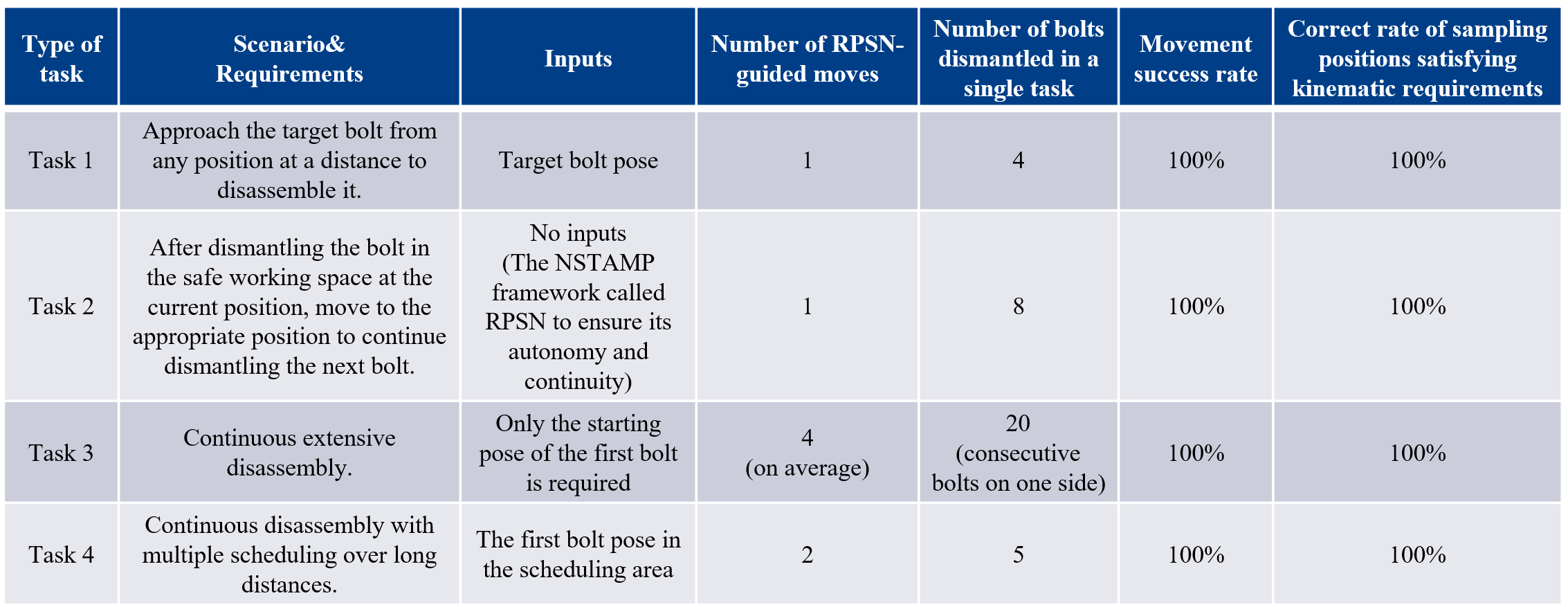
We deployed the RPSN for experiments in real-world scenarios, where the AGV is required to carry the UR10e to autonomously disassemble the surface bolts of the EOL-EVB. The RPSN is utilized in the NeuroSymbolic TAMP framework [22] and acts as the primitive ”Approach ” in guiding the entire autonomous movement of the AGV chassis. To comprehensively assess the performance of RPSN across various usage scenarios, we formulated four tasks. The corresponding task scenarios and requirements are illustrated in Figure 8. Through over 80 times of real-machine experiments, we observed that the RPSN accurately samples positions in actual disassembly scenarios with a 100% success rate. This achievement is attributed to both the high accuracy of the RPSN and the feedback checking. Demonstration videos for the four tasks are accessible on the paper’s website(see https://sites.google.com/view/sjtu-rpsn).

During experiments in real-world scenarios, we identified certain safety concerns. While some positions provided by the RPSN meet the kinematic constraints, they may still exhibit a notable distance from the bolt location. If the arm extends beyond a specific length, the tilting moment becomes excessive, making the AGV prone to overturning and causing one side of the wheels to lift off the ground. Preventing such occurrences requires an analysis that integrates static stability margin(SSM), Tumble Stability Margin(TSM), and other metrics [36, 37, 38]. In this experiment, a distance clustering method is employed to establish a safety zone for the chassis. We contemplate incorporating these stability constraints into the training process of the network in a differentiable form in future work. Aiming to make them an inherent part of the network’s intuition, thereby enhancing safety during operational processes.

IV-D Summary of Experiments

Experimental data shows that in the EOL-EVB disassembly scenario, RPSN can reliably determine the target chassis position for a given bolt without the need for sampling, planning, or simulation. The robot has a probability of completing the disassembly work directly in the position with a probability of 96.67%. The Differentiable Kinematics Calculation Engine can also act as a feedback check. Even in the event of an initial sample failure, the RPSN possesses the capability to swiftly re-sample, ensuring the generation of a reliable position with a 100% success rate. RPSN1 has an average sampling number of only 1.28 out of the 300 times of test data which will save a large amount of arithmetic power compared to the random sampling method which has 31.04 iterations of attempts and simulations.

The applications of this network model extend beyond battery pack disassembly. It pertains to all scenarios involving mobile robot motion planning, encompassing target position selection, forward and reverse kinematics, which are precisely the problems addressed by RPSN. Similar to humans, a robotic arm is akin to a human arm. Just as humans instinctively understand how their legs must position themselves to enable their arms to reach, grasp, and stably hold an object on a distant table. In contrast, robotic arms have fewer degrees of freedom and can suffer from kinematic singularities. With the help of the RPSN, the robot overcomes these problems well and seems to be able to have subconscious decision-making, which is just in line with the cognitive and embodied intelligence of robots in the NeuroSymbolic AI framework.

V Conclusions

Mobile robot motion planning often requires numerous iterations of random sampling and kinematic simulation to pinpoint the target chassis’s position. To address this problem, we designed RPSN based on the concept of the NeuroSymbolic AI. The RPSN, comprising a Position Prediction Network and a Differentiable Kinematics Calculation Engine, can directly output a highly plausible chassis position, given the pose of the working object, under which the robot kinematics is guaranteed to have a solution. We deployed the RPSN on EOL-EVB disassembly application scenarios. Our rigorous experimental validation in End-of-Life Vehicle Battery (EOL-EVB) disassembly application scenarios demonstrated that the RPSN can achieve an impressive 96.67% accuracy in initially determining the target chassis location. Furthermore, iterative sampling consistently provides 100% valid chassis locations, averaging 1.28 times.

In this study, We pioneered an approach integrating robots’ forward and backward kinematics into the neural network’s computational graph through differentiable programming. This integration redefines the traditional neural network training paradigm, significantly reducing the dependency on data during training. It opens a door for our future research, integrating differentiated classical algorithms with neural networks and rapidly guiding the learning of reliable speculative neural networks through mature knowledge. In the next step, we will attempt to introduce collision detection into the system, further enhancing the agility of robots and contributing to the advancement of embodied intelligence.

References

- [1] Benjamin Burger, Phillip M Maffettone, Vladimir V Gusev, Catherine M Aitchison, Yang Bai, Xiaoyan Wang, Xiaobo Li, Ben M Alston, Buyi Li, Rob Clowes, et al. A mobile robotic chemist. Nature, 583(7815):237–241, 2020.
- [2] Kathrin Dörfler, Gido Dielemans, Lukas Lachmayer, Tobias Recker, Annika Raatz, Dirk Lowke, and Markus Gerke. Additive manufacturing using mobile robots: Opportunities and challenges for building construction. Cement and Concrete Research, 158:106772, 2022.
- [3] Luke Antonyshyn, Jefferson Silveira, Sidney Givigi, and Joshua Marshall. Multiple mobile robot task and motion planning: A survey. ACM Computing Surveys, 55(10):1–35, 2023.
- [4] Emrah Akin Sisbot, Luis F Marin-Urias, Rachid Alami, and Thierry Simeon. A human aware mobile robot motion planner. IEEE Transactions on Robotics, 23(5):874–883, 2007.
- [5] Runqi Chai, Hanlin Niu, Joaquin Carrasco, Farshad Arvin, Hujun Yin, and Barry Lennox. Design and experimental validation of deep reinforcement learning-based fast trajectory planning and control for mobile robot in unknown environment. IEEE Transactions on Neural Networks and Learning Systems, 2022.
- [6] Caelan Reed Garrett, Rohan Chitnis, Rachel Holladay, Beomjoon Kim, Tom Silver, Leslie Pack Kaelbling, and Tomás Lozano-Pérez. Integrated task and motion planning. Annual review of control, robotics, and autonomous systems, 4:265–293, 2021.
- [7] Zi Wang, Caelan Reed Garrett, Leslie Pack Kaelbling, and Tomás Lozano-Pérez. Learning compositional models of robot skills for task and motion planning. The International Journal of Robotics Research, 40(6-7):866–894, 2021.
- [8] Jeongmin Jeon, Hong-ryul Jung, Francisco Yumbla, Tuan Anh Luong, and Hyungpil Moon. Primitive action based combined task and motion planning for the service robot. Frontiers in Robotics and AI, 9:713470, 2022.
- [9] Zhutian Yang, Caelan Reed Garrett, and Dieter Fox. Sequence-based plan feasibility prediction for efficient task and motion planning. arXiv preprint arXiv:2211.01576, 2022.
- [10] Beomjoon Kim, Zi Wang, Leslie Pack Kaelbling, and Tomás Lozano-Pérez. Learning to guide task and motion planning using score-space representation. The International Journal of Robotics Research, 38(7):793–812, 2019.
- [11] Sergio Cebollada, Luis Payá, María Flores, Adrián Peidró, and Oscar Reinoso. A state-of-the-art review on mobile robotics tasks using artificial intelligence and visual data. Expert Systems with Applications, 167:114195, 2021.
- [12] Ahmed Hussain Qureshi, Yinglong Miao, Anthony Simeonov, and Michael C Yip. Motion planning networks: Bridging the gap between learning-based and classical motion planners. IEEE Transactions on Robotics, 37(1):48–66, 2020.
- [13] Garcez Artur d’Avila, Raedt Luc De, Földiak Peter, Hitzler Pascal, Icard Thomas, Kühnberger Kai-Uwe, Miikkulainen Risto, et al. Neural-symbolic learning and reasoning: contributions and challenges. In AAAI Spring Symposium Series, AAAI Press, Palo Alto, California, USA, pages 20–23, 2015.
- [14] Bo Zhang, Jun Zhu, and Hang Su. Toward the third generation artificial intelligence. Science China Information Sciences, 66(2):121101, 2023.
- [15] Artur d’Avila Garcez and Luis C Lamb. Neurosymbolic ai: The 3 rd wave. Artificial Intelligence Review, pages 1–20, 2023.
- [16] Hsiao-Ying Lin. Team with the strong, work with the wise. Computer, 56(7):116–120, 2023.
- [17] Y LeCun. Deep learning has outlived its usefulness as a buzz-phrase, 2018.
- [18] Yoshua Bengio et al. From system 1 deep learning to system 2 deep learning. In Neural Information Processing Systems, 2019.
- [19] Constructions Aeronautiques, Adele Howe, Craig Knoblock, ISI Drew McDermott, Ashwin Ram, Manuela Veloso, Daniel Weld, David Wilkins SRI, Anthony Barrett, Dave Christianson, et al. Pddl— the planning domain definition language. Technical Report, Tech. Rep., 1998.
- [20] Caelan Reed Garrett, Tomás Lozano-Pérez, and Leslie Pack Kaelbling. Pddlstream: Integrating symbolic planners and blackbox samplers via optimistic adaptive planning. In Proceedings of the International Conference on Automated Planning and Scheduling, volume 30, pages 440–448, 2020.
- [21] Wei Ren, Zhigang Wang, Hua Yang, Yisheng Zhang, and Ming Chen. Neurosymbolic task and motion planner for disassembly electric vehicle batteries. J. Comput. Res. Dev, 58:2604, 2021.
- [22] Hengwei Zhang, Yisheng Zhang, Zhigang Wang, Shengmin Zhang, Huaicheng Li, and Ming Chen. A novel knowledge-driven flexible human–robot hybrid disassembly line and its key technologies for electric vehicle batteries. Journal of Manufacturing Systems, 68:338–353, 2023.
- [23] Hengwei Zhang, Hua Yang, Haitao Wang, Zhigang Wang, Shengmin Zhang, and Ming Chen. Autonomous electric vehicle battery disassembly based on neurosymbolic computing. In Proceedings of SAI Intelligent Systems Conference, pages 443–457. Springer, 2022.
- [24] Yisheng Zhang, Hengwei Zhang, Zhigang Wang, Shengmin Zhang, Huaicheng Li, and Ming Chen. Development of an autonomous, explainable, robust robotic system for electric vehicle battery disassembly. In 2023 IEEE/ASME International Conference on Advanced Intelligent Mechatronics (AIM), pages 409–414. IEEE, 2023.
- [25] Kimitoshi Yamazaki, Satoshi Suzuki, and Yusuke Kuribayashi. Approaching motion planning for mobile manipulators considering the uncertainty of self-positioning and object’s pose estimation. Robotics and Autonomous Systems, 158:104232, 2022.
- [26] Martin Sereinig, Wolfgang Werth, and Lisa-Marie Faller. A review of the challenges in mobile manipulation: systems design and robocup challenges. Elektrotech. Informationstechnik, 137(6):297–308, 2020.
- [27] Mingyi Zhang, Xilong Liu, De Xu, Zhiqiang Cao, and Junzhi Yu. Vision-based target-following guider for mobile robot. IEEE Transactions on Industrial Electronics, 66(12):9360–9371, 2019.
- [28] Mohamed Khodeir, Ben Agro, and Florian Shkurti. Learning to search in task and motion planning with streams. IEEE Robotics and Automation Letters, 8(4):1983–1990, 2023.
- [29] Sebastian Christodoulou and Uwe Naumann. Differentiable programming: Efficient smoothing of control-flow-induced discontinuities. arXiv preprint arXiv:2305.06692, 2023.
- [30] Hai-Jun Liao, Jin-Guo Liu, Lei Wang, and Tao Xiang. Differentiable programming tensor networks. Physical Review X, 9(3):031041, 2019.
- [31] Tzu-Mao Li, Michaël Gharbi, Andrew Adams, Frédo Durand, and Jonathan Ragan-Kelley. Differentiable programming for image processing and deep learning in halide. ACM Transactions on Graphics (ToG), 37(4):1–13, 2018.
- [32] Mike Innes, Alan Edelman, Keno Fischer, Chris Rackauckas, Elliot Saba, Viral B Shah, and Will Tebbutt. A differentiable programming system to bridge machine learning and scientific computing. arXiv preprint arXiv:1907.07587, 2019.
- [33] Jacques Denavit and Richard S Hartenberg. A kinematic notation for lower-pair mechanisms based on matrices. 1955.
- [34] CR Rocha, CP Tonetto, and Altamir Dias. A comparison between the denavit–hartenberg and the screw-based methods used in kinematic modeling of robot manipulators. Robotics and Computer-Integrated Manufacturing, 27(4):723–728, 2011.
- [35] Richard Liaw, Eric Liang, Robert Nishihara, Philipp Moritz, Joseph E Gonzalez, and Ion Stoica. Tune: A research platform for distributed model selection and training. arXiv preprint arXiv:1807.05118, 2018.
- [36] Mahdi Agheli and Stephen S Nestinger. Force-based stability margin for multi-legged robots. Robotics and Autonomous Systems, 83:138–149, 2016.
- [37] Antonio Diaz-Calderon and Alonzo Kelly. On-line stability margin and attitude estimation for dynamic articulating mobile robots. The International Journal of Robotics Research, 24(10):845–866, 2005.
- [38] Zhihua Chen, Jiehao Li, Shoukun Wang, Junzheng Wang, and Liling Ma. Flexible gait transition for six wheel-legged robot with unstructured terrains. Robotics and Autonomous Systems, 150:103989, 2022.