Radar Anti-jamming Strategy Learning via Domain-knowledge Enhanced Online Convex Optimization

Abstract

The dynamic competition between radar and jammer systems presents a significant challenge for modern Electronic Warfare (EW), as current active learning approaches still lack sample efficiency and fail to exploit jammer’s characteristics. In this paper, the competition between a frequency agile radar and a Digital Radio Frequency Memory (DRFM)-based intelligent jammer is considered. We introduce an Online Convex Optimization (OCO) framework designed to illustrate this adversarial interaction. Notably, traditional OCO algorithms exhibit suboptimal sample efficiency due to the limited information obtained per round. To address the limitations, two refined algorithms are proposed, utilizing unbiased gradient estimators that leverage the unique attributes of the jammer system. Sub-linear theoretical results on both static regret and universal regret are provided, marking a significant improvement in OCO performance. Furthermore, simulation results reveal that the proposed algorithms outperform common OCO baselines, suggesting the potential for effective deployment in real-world scenarios.

Index Terms—  frequency-agile radar, anti-jamming, online convex optimization, regret analysis

1 Introduction

The evolution of electronic warfare (EW) has introduced significant challenges for modern radar systems, especially due to the emergence of intelligent jammers [1, 2]. Among them, main lobe jamming poses a severe threat as jammers deliberately position themselves within the radar’s main beam. Traditional signal processing techniques developed to detect and mitigate jamming signals often fall short, as they rely on specific assumptions that may not always be valid. For example, blind source separation assumes a non-zero angular separation between the radar and jammer[3], which is invalid in scenarios involving self-protection jammers [4].

To address the limitations of traditional jamming countermeasures, frequency agility has been adopted, enabling radar systems to implement adaptive frequency hopping strategies in the face of main lobe jamming [5, 6, 7]. Recently, the application of learning techniques has redefined anti-jamming efforts as sequential decision-making problems. In particular, reinforcement learning has been incorporated into the development of anti-jamming strategies, with notable research exploring the deployment of Deep Q-Networks (DQN) [8, 9]. Game-theoretic methods, including two-person zero-sum games and extensive-form games with imperfect information, have been leveraged to enhance strategic anti-jamming performance [10, 11, 12]. Additionally, the multi-armed bandit framework has emerged as a novel approach for designing anti-jamming strategies [13, 14]. The field continues to advance with studies on subpulse-level frequency agile radar systems [15] and the development of adaptive power allocation models for jammers [11]. However, these active online learning techniques in anti-jamming strategy design either fall short in sample efficiency or struggle to model the dynamics of the jammer.

To overcome these limitations, it is essential to effectively model the attributes of the jammer system. In this paper, we adopt the framework of Online Convex Optimization (OCO) [16], in which the jamming strategy can be naturally embedded in the gradient of the cost function. The online interaction information thus can be effectively utilized to estimate the gradient and a online mirror descent algorithm is developed. We show that for an arbitrary jammer, the developed algorithm achieves $O(\sqrt{N})$ static regret bound (comparing with the best fixed decision in hindsight), where $N$ is the total number of iterations. This improves the results of existing works [17, 18, 19]. Further, by exploiting the knowledge that the jammer’s decisions are predicated on past interactions, we devise a more efficient algorithm that achieves an $O(\sqrt{N})$ regret bound for universal regret. This sub-linear performance suggests the feasibility of reaching an optimal anti-jamming strategy and marks a significant improvement over classic OCO algorithms. The simulation results further demonstrates that proposed algorithms outperforms OCO baselines.

2 System Model

2.1 Signal Model

Consider a frequency-agile radar system that employs a subpulse-level frequency-agile waveform during transmission. The system works in a monopulse mode, a single pulse is composed of multiple sub-pulses, each operating at a unique carrier frequency. Let $\mathcal{F}=\{f_{1},f_{2},\ldots,f_{L}\}$ denote the set of available carrier frequencies, with each frequency $f_{i}$, $i=2,3,\ldots,L$, defined as $f_{i-1}+\Delta f$ and $\Delta f$ represents the frequency step size. Denoting $M$ as the total number of sub-pulses within one pulse, the transmitted frequency-agile signal of the $n$-th pulse $(n\in[N])$ at time $t$ is expressed as

$$s_{n}(t)=\sum_{m=0}^{M-1}\text{rect}\left(\frac{t-mT_{c}}{T_{c}}\right)P_{m}a(t)\exp{(j2\pi f^{\textrm{R}}_{m}t)},$$ (1)

where $T_{c}$ is the sub-pulse duration, $P_{m}$ represents the power allocated to the $m$-th subpulse, $a(t)$ is the complex envelope, and $\text{rect}(t)$ is the rectangle function defined as $\text{rect}(t)=1$ for $0\leq t\leq 1$ and $\text{rect}(t)=0$ otherwise. Parameter $f^{\textrm{R}}_{m}\in\mathcal{F}$ denotes the sub-carrier frequency for the $m$-th sub-pulse, which may vary among sub-pulses.

The jamming system is equipped on the target, aims to mask the radar’s reflected pulse echo by transmitting a noise-modulated signal. The distance between the radar and target/jammer is denoted as $R$, and the jamming signal $j_{n}(t)$ can be described as

$$j_{n}(t)=\sum_{m=0}^{M-1}\text{rect}\left(\frac{t-T_{d}-mT_{c}}{T_{c}}\right)b_{m}(t)\exp{(j2\pi f^{\mathrm{J}}_{m}t)}$$ (2)

where $T_{d}=R/c$ ($c$ is the speed of light) is the propagation delay from the radar to the target/jammer, $b_{m}(t)$ represents the noise-modulated envelope, and $f^{\textrm{J}}_{m}$ corresponds to the carrier frequency of sub-pulse $m$. At the receiver, the radar captures a signal mixture consisting of the reflected radar pulse echo, the jamming signal, and additive noise. The received signal $r_{n}(t)$ is expressed as

$$r_{n}(t)=s_{n}(t-T_{d})+j_{n}(t-T_{d})+w_{n}(t),$$ (3)

where $w_{n}(t)$ denotes the additive white Gaussian noise.

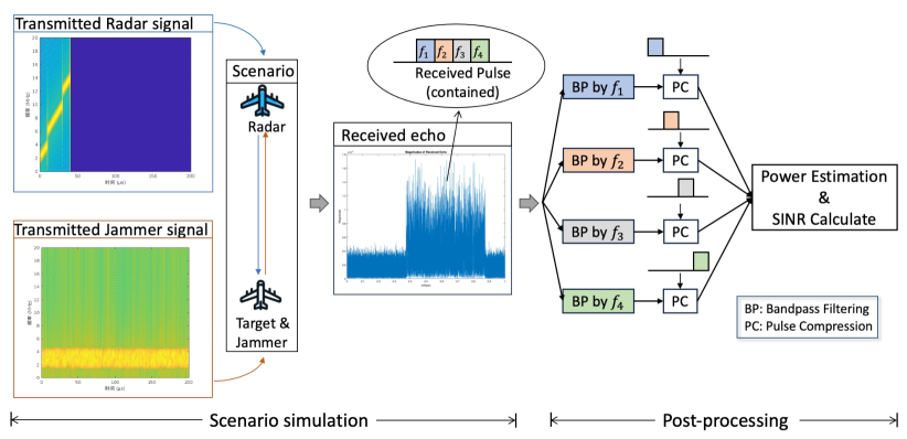
Fig. 1: A detailed illustration on the anti-jamming scenario

2.2 Post-processing of Received Signal

By implementing a suitable post-processing procedure on the mixed signal $r_{n}(t)$, it is possible to extract valuable information of the jamming signal and the radar echo. This procedure involves bandpass filtering to isolate the desired frequency band, followed by matched filtering designed to enhance the of subpulses in radar echo. The sequential steps of this procedure are depicted in the flowchart presented in Fig. 1. Crucially, this process facilitates the estimation of the power of each subpulses in radar echo, denoted as $P_{\mathrm{R}}(f^{\mathrm{R}}_{m})$, the power of jamming signal in radar receiver $P_{\mathrm{J}}$, and the noise power $P_{n_{0}}$. Consequently, the Signal-to-Interference-plus-Noise Ratio (SINR) for each subpulse $m$ can be calculated, denoted as $\text{SINR}_{m}$,

$$\text{SINR}_{m}=\frac{P_{\mathrm{R}}(f^{\mathrm{R}}_{m})}{P_{n_{0}}+P_{\mathrm{J}}\mathbf{1}(f^{\mathrm{R}}_{m}=f^{\mathrm{J}}_{m})},$$ (4)

where the indicator function $\mathbf{1}(f^{\mathrm{R}}_{m}=f^{\mathrm{J}}_{m})$ determines whether the received echo is subject to jamming on sub-pulse $m$. $\text{SINR}_{m}$ indicates the quality of the $m$-th sub-pulse for target detection, which will be used as the utility function later.

3 OCO-based Radar Strategy Design

3.1 Online Optimization Formulation

Based on the established signal models and post-processing procedure in Section 2, each pulse can be regarded as one round of interaction between the radar and jammer. Protocol 1 presents the protocol for this type of iterative interaction. The radar system dynamically adjusts its transmitted signal $s_{n}(t)$ to improve the SINR, by utilizing information extracted from previous pulses. To systematically select parameters of $s_{n}(t)$ at each iteration for this online interaction process, we propose an online optimization framework from the radar’s perspective. The goal is to enhance the radar’s adaptive capabilities in response to jammer, ensuring that with each pulse, the radar’s response is optimally adjusted to the evolving jamming strategies. Basic elements involved in this online interaction process are given below.

Algorithm 1 Iterative anti-jamming procedure

for pulse $n=1,2,\ldots,N$ do

    Radar transmits the signal $s_{n}(t)$;

    Jammer detects $s_{n}(t)$ and immediately transmits $j_{n}(t)$;

    Radar receives the echo $r_{n}(t)$ and calculate SINR from it.

end for

• Radar’s action $a_{n}$: $a_{n}=(f^{\mathrm{R}}_{n,1},f^{\mathrm{R}}_{n,2},\ldots,f^{\mathrm{R}}_{n,M})\in\mathcal{A}_{\mathrm{R}}=\mathcal{F}^{M}$ represents the radar’s choice of various sub-carrier frequencies at the $n$-th pulse.

• Radar’s strategy $\boldsymbol{x}_{n}$: The strategy from which $a_{n}$ is selected belongs to the probability simplex $\Delta_{|\mathcal{A}_{\mathrm{R}}|}$.

• Cost function $f_{n}$: The convex cost function takes a linear form as $f_{n}(\boldsymbol{x})=\langle\boldsymbol{\ell}_{n},\boldsymbol{x}\rangle:\Delta_{|\mathcal{A}_{\mathrm{R}}|}\rightarrow\mathbb{R}$.

Notably, for each pulse $n$, only $\boldsymbol{\ell}(a_{n})\in[0,1]$ is accessible, derived from (4) as

$$\boldsymbol{\ell}(a_{n})=\frac{c-\text{SINR}(a_{n})}{c}\in[0,1],$$ (5)

where $c$ is an SINR threshold that indicates high enough detection probability, $\text{SINR}(a_{n})=\frac{1}{M}\sum_{m=1}^{M}\min(\text{SINR}_{m}(a_{n}),c)$, and $\text{SINR}_{m}(a_{n})$ is the SINR of the $m$-th pulse associating with action $a_{n}$ (c.f. (4)). For the $n$-th pulse, radar’s goal is to find a strategy $\boldsymbol{x}_{n}$ that minimizes the cost function $f_{n}$ and the optimization problem is

$$\min_{\boldsymbol{x}_{n}} f_{n}(\boldsymbol{x}_{n})$$ (6)

s.t. $$\boldsymbol{x}_{n}\in\Delta_{|\mathcal{A}_{\mathrm{R}}|}.$$

Achieving the optimal solution $\boldsymbol{x}^{*}_{n}$ poses a significant challenge due to the dynamic and unknown nature of $f_{n}$. Consequently, for each pulse $n$, an implementable online algorithm $\mathcal{A}$ is employed. This algorithm uses the historical function values $(f_{1},f_{2},\ldots,f_{n-1})$, along with any other pertinent information, to generate the strategy $\boldsymbol{x}_{n}$. The action $a_{n}$ is then selected according to the probability distribution defined by $\boldsymbol{x}_{n}$. After executing the algorithm over $N$ pulses, the retrospectively best strategy $\boldsymbol{x}^{*}$ is defined as $\boldsymbol{x}^{*}=\arg\min_{\boldsymbol{x}\in\Delta_{|\mathcal{A}_{R}|}}\sum_{n=1}^{N}f_{n}(\boldsymbol{x})$. A meaningful performance metric for the online algorithm $\mathcal{A}$ is the so-called static regret. This metric evaluates the cumulative cost incurred by algorithm $\mathcal{A}$ and compares it with the cost of $\boldsymbol{x}^{*}$,

$$\text{S-Regret}_{N}(\mathcal{A})=\sum_{n=1}^{N}f_{n}(\boldsymbol{x}_{n})-\sum_{n=1}^{N}f_{n}(\boldsymbol{x}^{*}).$$ (7)

Algorithm $\mathcal{A}$ is said to be effective if its regret is sublinear as a function of $N$, i.e., $\text{S-Regret}_{N}(\mathcal{A})=o(N)$. This condition implies that on average, the algorithm performs as well as the best fixed strategy in hindsight.

3.2 Online Mirror Descent

Based on E.q. (7), the Online Gradient Descent (OGD)[16] can be used for updating $\boldsymbol{x}_{n}$, given as

$$\boldsymbol{x}_{n+1}=\text{Proj}_{\Delta_{|\mathcal{A}_{\mathrm{R}}|}}[\boldsymbol{x}_{n}-\eta_{n}\nabla f_{n}(\boldsymbol{x}_{n})]$$ (8)

where $\text{Proj}{\Delta_{|\mathcal{A}_{\mathrm{R}}|}}[\cdot]$ represents projection onto the feasible set $\Delta_{|\mathcal{A}_{\mathrm{R}}|}$, and $\eta_{n}$ is the learning rate at iteration $n$. To ensure stability [20] of OGD, a regularization term named Bregman divergence $D_{F}(\boldsymbol{x},\boldsymbol{x}_{n})$[21] is introduced, which is associated with a Legendre function $F$[22] and its domain $\mathcal{D}$. Consequently, the update rule becomes

$$\begin{cases}&\boldsymbol{u}_{n+1}=\operatorname*{argmin}\limits_{\boldsymbol{x}\in\mathcal{D}}\ \eta_{n}\langle\boldsymbol{x},\nabla f_{n}\rangle+D_{F}(\boldsymbol{x},\boldsymbol{x}_{n})\\ &\boldsymbol{x}_{n+1}=\operatorname*{argmin}\limits_{\boldsymbol{x}\in\Delta_{|\mathcal{A}_{\mathrm{R}}|}}\ D_{F}(\boldsymbol{x},\boldsymbol{u}_{n+1})\end{cases}$$ (9)

This iterative process is known as Online Mirror Descent (OMD) [23] and $F(x)=\sum(x_{i}\ln{x_{i}}-x_{i})$ is commonly adopted ($x_{i}$ is the $i$-th element of $x$), which admits analytic expression for (9). Notice that during the online interaction, only $f_{n}(a_{n})$ is observed, other values of $f_{n}(a),a\neq a_{n}$ are not available. This makes estimating $\nabla f_{n}$ be the key step of (9). A naive estimator is the importance weighted estimator (IWE) [24] given as

$$\boldsymbol{\hat{\ell}}_{n}(a)=\begin{cases}\frac{f_{n}(a)}{\boldsymbol{x}_{n}(a)},&a=a_{n}\\ 0,&\text{otherwise}.\end{cases}$$ (10)

Setting $\nabla f_{n}=\boldsymbol{\hat{\ell}}_{n}$, the OMD algorithm in (9) is equivalent to a classical bandit algorithm known as Exp3 [25], characterized by a sub-linear static regret bound of $\mathcal{O}(\sqrt{N|\mathcal{A}_{\mathrm{R}}|\log{|\mathcal{A}_{\mathrm{R}}|}})$. However, the IWE neglects the strategic nature of the interaction inherent in the online process, where the radar is essentially engaged in a game against a jammer. Critical insights into the jammer’s behavior remain unutilized. By incorporating knowledge about the jammer’s action space and strategy, we can develop more sophisticated and effective online algorithms.

4 Proposed Algorithms

4.1 Action Modeling

By leveraging the characteristics of the jammer, its action and strategy are modeled as below.

• Jammer’s action $b_{n}$: $b_{n}\in\mathcal{A}_{\mathrm{J}}=\mathcal{F}^{M}\cup\mathcal{B}$, where $\mathcal{B}$ represents specific jamming action such repeater jamming [26, 27].

• Jammer’s strategy $\boldsymbol{y}_{n}$: $b_{n}$ is selected from its strategy $\boldsymbol{y}_{n}\in\Delta_{|\mathcal{A}_{\mathrm{J}}|}$, where $\Delta_{|\mathcal{A}_{\mathrm{J}}|}$ denotes the probability simplex.

The cost function $f_{n}$ thus can be related to the cost of a two-player matrix game. In particular consider a matrix game with cost matrix $\textbf{U}\in\mathbb{R}^{|\mathcal{A}_{\mathrm{R}}|\times|\mathcal{A}_{\mathrm{J}}|}$, at the $n$-th pulse, the radar player takes action $a_{n}\sim\boldsymbol{x}_{n}$, the jammer player takes action $b_{n}\sim\boldsymbol{y}_{n}$, then the following holds

$$\mathbb{E}_{b_{n}\sim\boldsymbol{y}_{n}}[f_{n}(\boldsymbol{x}_{n})]=\boldsymbol{x}_{n}^{T}\textbf{U}\boldsymbol{y}_{n}:=\phi(\boldsymbol{x}_{n},\boldsymbol{y}_{n}),$$ (11)

The above claim implies that an unbiased gradient estimator of $f_{n}(\boldsymbol{x}_{n})$ can be attained as

$$\boldsymbol{\hat{\ell}}_{n}=\textbf{U}[:,b_{n}],$$ (12)

where the unbiased property is due to

$$\mathbb{E}[\boldsymbol{\hat{\ell}}_{n}]=\textbf{U}\times\mathbb{E}[\boldsymbol{b}_{n}]=\textbf{U}\times\boldsymbol{y}_{n}=\boldsymbol{\ell}_{n}.$$

$\boldsymbol{b}_{n}$ is the pure strategy of jammer related with its action $b_{n}\sim\boldsymbol{y}_{n}$.

By incorporating the gradient estimator from (12) into the OMD (9), we introduce an enhanced algorithm referred to as OMD with Action Modeling (OMD-AM), which is elaborated in Algorithm 1. OMD-AM achieves a sub-linear static regret bound $\mathcal{O}(\sqrt{N\log{|\mathcal{A}|}})$, with the proof omitted here. This improved regret bound effectively removes the square-root dependence on the size of the action set $|\mathcal{A}|$ that characterizes the classical Exp3 algorithm. The key to this advancement lies in leveraging the inherent game structure of the cost matrix.

Algorithm 1 Online Mirror Descent with Action Modeling(OMD-AM)

Input: $\eta>0$, $\boldsymbol{x}_{1}=(1/|\mathcal{A}_{\mathrm{R}}|)\times\mathbf{1}$

for pulse $n=1,2,\ldots,N$ Radar do

    Take action $a_{n}\sim\boldsymbol{x}_{n}$ and observe the echo $r_{n}(t)$;

    Gradient estimation from $r_{n}(t)$ by E.q. (12);

    Online mirror descent with $\boldsymbol{\hat{\ell}}_{n}$ by E.q. (9);

end for

4.2 Opponent Modeling

Modern jamming system usually contains a crucial subsystem named Digital Radio Frequency Memory (DRFM) [1], which records useful interaction histories that jammers can utilize to make informed decisions. By leveraging knowledge of the jamming strategy generation mechanism—specifically, the jamming strategy is a pre-defined fixed decision rule based on a length-$k$ history $h_{n}=\{a_{n-1},b_{n-1},\ldots,a_{n-k},b_{n-k}\}\in\mathcal{H}=\mathcal{A}_{\mathrm{R}}^{k}\times\mathcal{A}_{\mathrm{J}}^{k}$—a more effective online algorithm can be developed. Under this setting, jamming strategy $\boldsymbol{y}_{n}$ is re-expressed as

$$\boldsymbol{y}_{n}=\pi\left(h_{n}\right),$$

where $\pi:\mathcal{H}\rightarrow\Delta_{|\mathcal{A}_{\mathrm{J}}|}$ is defined as the mapping from history space to the jammer’s action space. Thus, the gradient estimator $\boldsymbol{\hat{\ell}}_{n}$ can be re-formulated by associating the length-$k$ history $h_{n}$,

$$\boldsymbol{\hat{\ell}}_{n}=\textbf{U}\boldsymbol{\hat{y}}_{n},$$ (13)

where $\boldsymbol{\hat{y}}_{n}=\pi_{n}(h_{n})$ represents the estimate of the decision rule $\pi$ at pulse $n$. A natural choice for $\pi_{n}$ is the maximum likelihood estimator (MLE), which calculates the frequency of each action $b\in\mathcal{A}_{\mathrm{J}}$, conditioned on a length-$k$ history $h\in\mathcal{H}$, across the entire interaction history $(a_{1},b_{1},\ldots,a_{n-1},b_{n-1})$. Combining gradient estimator (13) with OMD (9), we attain OMD with Opponent Modeling (OMD-OM), elaborated in Algorithm 2.

Notably, for OMD-OM, the static regret defined in (7) may tend to negative as it only compares with the best strategy $\boldsymbol{x}^{*}$ in hindsight. This comparator is weak since OMD-OM exploits the jammer strategy information. To address this limitation, we introduce a broader performance metric termed universal regret, which aligns more closely with the objective function described in (6).

$$\text{U-Regret}_{N}(\mathcal{A})=\sum_{n=1}^{N}f_{n}(\boldsymbol{x}_{n})-\min_{\boldsymbol{z}_{1},\ldots,\boldsymbol{z}_{N}}\sum_{n=1}^{N}f_{n}(\boldsymbol{z}_{n})$$ (14)

where $(\boldsymbol{z}_{1},\ldots,\boldsymbol{z}_{N})$ is a comparator sequence. Furthermore, if $\boldsymbol{z}_{1}=\ldots=\boldsymbol{z}_{N}=\boldsymbol{x}=\operatorname*{argmin}_{\boldsymbol{x}}\sum_{n=1}^{N}f_{n}(\boldsymbol{x})$, it reverts to static regret. Typically, achieving sub-linear universal regret is unattainable due to the unknown dynamics of the environment. Nevertheless, OMD-OM, which exploits the information of jamming strategy generation, utilizes a history-dependent predictor to capture the dynamic nature of the jamming strategy. By doing so, it can attain a sub-linear universal regret bound, expressed as $\mathcal{O}(\sqrt{N|\mathcal{H}|\log{|\mathcal{A}_{\mathrm{R}}|}})$ with the proof omitted here. This bound represents a significant improvement over the sub-linear static regret bounds obtained with Exp3 and OMD-AM, offering a mechanism to adapt to the dynamics of jamming environments effectively.

Algorithm 2 Online Mirror Descent with Opponent Modeling (OMD-OM)

Input: $\boldsymbol{x}_{1}$, length-$k$ history $\mathcal{H}$.

for pulse $n=1,2,\ldots,N$ Radar do

    Take action $a_{n}\sim\boldsymbol{x}_{n}$ and observe the echo $r_{n}(t)$;

    Update the history $\mathcal{H}$ and obtain $\boldsymbol{\hat{y}}_{n}$ by MLE;

    Gradient estimation by E.q. (13);

    Online mirror descent with $\boldsymbol{\hat{\ell}}_{n}$ by E.q. (9);

end for

5 Experiments

Parameter	Value
Radar antenna gain	30dB
Radar transmitted power $P_{R}$	10KW
Jammer transmitted power $P_{J}$	1KW
# of sub-pulses	4
Sub-pulse width	3$\mu$s
PRF	1000Hz
Carrier frequency	10GHz
Distance	100KM

Table 1: Parameter setting for FA radar and jammer.

This section evaluates the efficiency of the developed OMD-AM and OMD-OM algorithms through simulation experiments. Detailed settings for the radar and jammer systems are provided in Table 1. The static regret (7) and universal regret (14) are employed as the performance metrics. Two different jamming strategies were simulated: a stationary strategy where $\boldsymbol{y}_{n}=\boldsymbol{y}$ remains constant for all iterations within the simplex $\Delta_{|\mathcal{A}_{J}|}$, and a non-stationary strategy that varies in response to recent length-$3$ history, denoted as $\boldsymbol{y}_{n}=\pi(h_{n}),h_{n}\in\mathcal{H}$. Specifically, $\boldsymbol{y}_{n}(b_{1})=0.7$ and $\boldsymbol{y}_{n}(b_{2})=0.3$ where $b_{1},b_{2}$ are related with the two most common frequencies in $h_{n}$. The Exp3 algorithm serves as the baseline for comparison. For each algorithm, 500 independent trials are conducted, and the shaded areas in Fig.2 represent the confidence intervals of these trials.

Fig. 2(a) compares the average static regret under the stationary jamming strategy. The results indicate that all the evaluated algorithms achieve sub-linear regret. Notably, both OMD-OM and OMD-AM algorithms outperform the baseline Exp3 algorithm and OMD-OM significantly reduces the number of samples.

In Fig. 2(b), both the static and universal regrets for different algorithms under a non-stationary jamming strategy are compared. With regard to static regret, the OMD-AM algorithm exhibits a more rapid decline compared to the baseline Exp3, indicating a faster convergence rate. Notably, the OMD-OM algorithm demonstrates a substantial reduction in static regret, highlighting its smaller cumulative cost compared with the optimal static strategy. For universal regret, only OMD-OM achieves a sub-linear regret, showcasing its impressive capability to adapt to non-stationary environments.

Finally, Tab. 2 compares the instantaneous cost incurred by different algorithms under both stationary and non-stationary jamming strategies, evaluated after $1000$ rounds. The costs are calculated from E.q. (5). This table clearly underscores the superior performance of the OMD-AM and OMD-OM algorithms under different jamming strategies.

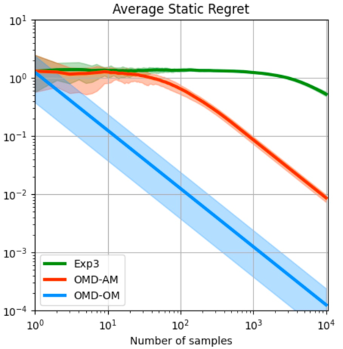
(a) Stationary jamming strategy.

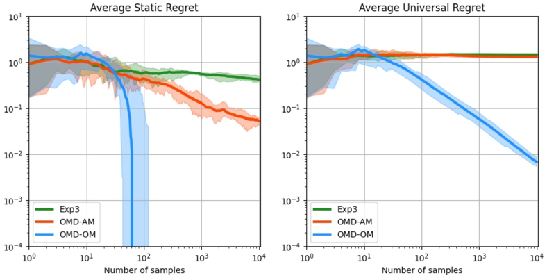
(b) Non-stationary jamming strategy.

Fig. 2: Comparison analysis of three algorithms under two different jamming strategies.

Jamming strategy	Exp3	OMD-AM	OMD-OM
Stationary	0.25	0	0
Non-stationary	0.42	0.34	0.09

Table 2: Instantaneous costs for various algorithms after $1000$ rounds.

6 Conclusion

This paper formulates the competition between subpulse-level frequency-agile radar and main-lobe intelligent jammer as an online convex optimization problem. Through careful modelings of the jamming strategies, we have developed algorithms that outperform conventional OCO benchmarks. Sub-linear static and universal regret bounds are provided, and numerical simulations demonstrates a significant enhancement in sample efficiency.

References

- [1] A. De Martino, Introduction to modern EW systems. Artech house, 2018.
- [2] D. Adamy, EW 101: A first course in electronic warfare. Artech house, 2001, vol. 101.
- [3] M. Ge, G. Cui, X. Yu, D. Huang, and L. Kong, “Mainlobe jamming suppression via blind source separation,” in 2018 IEEE Radar Conference (RadarConf18). Oklahoma City, OK: IEEE, Apr. 2018, pp. 0914–0918.
- [4] M. I. Skolnik, “Radar handbook,” 1970.
- [5] S. R. J. Axelsson, “Analysis of Random Step Frequency Radar and Comparison With Experiments,” IEEE Transactions on Geoscience and Remote Sensing, vol. 45, no. 4, pp. 890–904, Apr. 2007.
- [6] Z. Ruixue, X. Guifen, Z. Yue, and L. Hengze, “Coherent signal processing method for frequency-agile radar,” in 2015 12th IEEE International Conference on Electronic Measurement & Instruments (ICEMI), vol. 1. IEEE, 2015, pp. 431–434.
- [7] M. Bica and V. Koivunen, “Generalized Multicarrier Radar: Models and Performance,” IEEE Transactions on Signal Processing, vol. 64, no. 17, pp. 4389–4402, Sep. 2016.
- [8] Z. Zheng, W. Li, and K. Zou, “Airborne Radar Anti-Jamming Waveform Design Based on Deep Reinforcement Learning,” Sensors, vol. 22, no. 22, p. 8689, Nov. 2022.
- [9] K. Li, B. Jiu, P. Wang, H. Liu, and Y. Shi, “Radar active antagonism through deep reinforcement learning: A Way to address the challenge of mainlobe jamming,” Signal Processing, vol. 186, p. 108130, Sep. 2021.
- [10] X. Song, P. Willett, S. Zhou, and P. B. Luh, “The MIMO Radar and Jammer Games,” IEEE Transactions on Signal Processing, vol. 60, no. 2, pp. 687–699, Feb. 2012.
- [11] J. Geng, B. Jiu, K. Li, Y. Zhao, H. Liu, and H. Li, “Radar and Jammer Intelligent Game under Jamming Power Dynamic Allocation,” Remote Sensing, vol. 15, no. 3, p. 581, Jan. 2023.
- [12] K. Li, B. Jiu, W. Pu, H. Liu, and X. Peng, “Neural Fictitious Self-Play for Radar Antijamming Dynamic Game With Imperfect Information,” IEEE Transactions on Aerospace and Electronic Systems, vol. 58, no. 6, pp. 5533–5547, Dec. 2022.
- [13] Y. Fang, L. Zhang, S. Wei, T. Wang, and J. Wu, “Online Frequency-Agile Strategy for Radar Detection Based on Constrained Combinatorial Non-Stationary Bandit,” IEEE Transactions on Aerospace and Electronic Systems, pp. 1–15, 2022.
- [14] Y. Li, L. Liu, W. Pu, H. Liang, and Z.-Q. Luo, “Optimistic thompson sampling for no-regret learning in unknown games,” 2024. [Online]. Available: https://arxiv.org/abs/2402.09456
- [15] K. Li, B. Jiu, and H. Liu, “Deep Q-Network based Anti-Jamming Strategy Design for Frequency Agile Radar,” in 2019 International Radar Conference (RADAR). TOULON, France: IEEE, Sep. 2019, pp. 1–5.
- [16] M. Zinkevich, “Online convex programming and generalized infinitesimal gradient ascent,” in Proceedings of the 20th international conference on machine learning (icml-03), 2003, pp. 928–936.
- [17] E. Hazan, A. Agarwal, and S. Kale, “Logarithmic regret algorithms for online convex optimization,” Machine Learning, vol. 69, pp. 169–192, 2007.
- [18] S. Shalev-Shwartz et al., “Online learning and online convex optimization,” Foundations and Trends® in Machine Learning, vol. 4, no. 2, pp. 107–194, 2012.
- [19] A. Mokhtari, S. Shahrampour, A. Jadbabaie, and A. Ribeiro, “Online optimization in dynamic environments: Improved regret rates for strongly convex problems,” in 2016 IEEE 55th Conference on Decision and Control (CDC). IEEE, 2016, pp. 7195–7201.
- [20] E. Hazan et al., “Introduction to online convex optimization,” Foundations and Trends® in Optimization, vol. 2, no. 3-4, pp. 157–325, 2016.
- [21] A. Banerjee, S. Merugu, I. S. Dhillon, J. Ghosh, and J. Lafferty, “Clustering with bregman divergences.” Journal of machine learning research, vol. 6, no. 10, 2005.
- [22] H. H. Bauschke, J. M. Borwein et al., “Legendre functions and the method of random bregman projections,” Journal of convex analysis, vol. 4, no. 1, pp. 27–67, 1997.
- [23] E. Hazan and S. Kale, “Extracting certainty from uncertainty: Regret bounded by variation in costs,” Machine learning, vol. 80, pp. 165–188, 2010.
- [24] A. D. Flaxman, A. T. Kalai, and H. B. McMahan, “Online convex optimization in the bandit setting: gradient descent without a gradient,” arXiv preprint cs/0408007, 2004.
- [25] P. Auer, N. Cesa-Bianchi, Y. Freund, and R. E. Schapire, “The nonstochastic multiarmed bandit problem,” SIAM journal on computing, vol. 32, no. 1, pp. 48–77, 2002.
- [26] X. Wang, J. Liu, W. Zhang, Q. Fu, Z. Liu, and X. Xie, “Mathematic principles of interrupted-sampling repeater jamming (ISRJ),” Science in China Series F: Information Sciences, vol. 50, no. 1, pp. 113–123, Feb. 2007.
- [27] D. Feng, L. Xu, X. Pan, and X. Wang, “Jamming Wideband Radar Using Interrupted-Sampling Repeater,” IEEE Transactions on Aerospace and Electronic Systems, vol. 53, no. 3, pp. 1341–1354, Jun. 2017.