Giant resonant skew scattering of plasma waves in graphene off a micromagnet

Abstract

Electron skew scattering by impurities is one of the major mechanisms behind the anomalous Hall effect in ferromagnetic nanostructures. It is particularly strong at the surface of topological insulators where the Dirac equation governs electron dynamics. Motivated by recently discovered mappings between hydrodynamics and spin-1 Dirac equations, we consider the scattering of plasma waves — propagating charge density oscillations — excited in graphene off a non-uniform magnetic field created by an adjacent circular micromagnet. The calculated scattering amplitude not only exhibits a giant asymmetry, or skewness, but is resonantly enhanced if the frequency of the incoming wave matches the frequency of the trapped mode circulating the micromagnet in only one direction. Furthermore, if the frequency of incoming waves exceeds the Larmor frequency, the angular distribution of scattered plasma waves is indistinguishable from the one of Dirac electrons at the surface of a topological insulator scattering off a magnetic impurity. The micrometer scale of the proposed setup enables direct investigations of individual skew scattering events previously inaccessible in electronic systems.

Introduction: Spin–orbit interactions give rise to a plethora of phenomena in solids and play a central role in magnetic-field-free spintronic devices. These interactions have a relativistic origin and are weak in conventional semiconductor nanostructures; yet, the interactions dominate the kinetic energy of Dirac electronic states at the surface of topological insulators, e.g., $\hbox{Bi}_{2}\hbox{Se}_{3}$ and $\hbox{Bi}_{2}\hbox{Te}_{3}$ Hasan and Kane (2010); Hasan and Moore (2011). The emergent spin–momentum locking leads to coupled charge and spin transport Burkov and Hawthorn (2010), strong inverse spin-galvanic effects Garate and Franz (2010), and a rich interplay with topological magnetic defects Hurst et al. (2015); Divic et al. (2022); Paul and Fu (2021); Kurebayashi and Nagaosa (2019) and spin waves Efimkin and Kargarian (2021); Kargarian et al. (2016); Martinez-Berumen et al. (2023) in the presence of long-range magnetic ordering Bhattacharyya et al. (2021). These effects can be exploited in low-energy electronic and spintronic applications Hirohata et al. (2020).

Asymmetric – or skew – impurity scattering is another prominent effect due to the interplay between spin–orbit interactions and magnetism, resulting in the anomalous Hall effect (AHE) Nagaosa et al. (2010). The average scattering angle for Dirac electrons has been found to be an order of magnitude larger than the typical angle observed in conventional semiconductor systems, and the enhanced AHE has already attracted much attention Culcer and Das Sarma (2011); Sabzalipour and Partoens (2019); Liu et al. (2018); Culcer et al. (2020). However, there are other contributions, Berry phase-induced intrinsic and side-jumps mechanisms, and their separation is not straightforward. Moreover, the AHE is usually measured via macroscopic current–voltage probes, which average over the macroscopic number of electronic collisions. It would be highly desirable to develop a platform in which the skew scattering of Dirac electrons is tunable and can be directly probed.

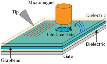
Figure 1: Schematic illustration of the considered setup. Plasma waves are excited in graphene by a near-field source and scatter off a non-uniform magnetic field created by an adjacent circular micromagnet. The calculated scattering amplitude has a high skewness and resonant behavior due to a single chiral interface mode (blue arrow line) circulating the micromagnet.

Recently, it has been realized that plasma waves (or plasmons) — propagating charge density oscillations — supported by a two-dimensional electron gas can be seen as distinct relatives of Dirac electrons Jin et al. (2016). The coupled hydrodynamic and Poisson equations describing their long-wavelength behavior can be reformulated as the relativistic-like pseudospin-1 Dirac equation. This mapping uncovered the topological stability of edge magnetoplasma waves Fetter (1985) and established the path toward their topological engineering Finnigan et al. (2022); Ciobanu et al. (2022); Sun et al. (2023); Van Mechelen et al. (2021). These findings naturally raise the question of whether the unexpected Dirac nature and resulting pseudospin–wavevector locking favor their skew scattering and whether such observations can provide helpful insights into the skew scattering of Dirac electrons.

In the present Letter, we consider plasma wave scattering in the setup sketched in Fig. 1. Propagating plasma waves in gated graphene, which is a unique, tunable, low-loss plasmonic material Grigorenko et al. (2012); Fei et al. (2012); Chen et al. (2012), are excited via a near-field source (e.g, a capacitive injector or atomic force microscope tip). The waves scatter off a non-uniform magnetic field created by an adjacent circular micromagnet. The calculated angular scattering distribution has a giant skewness, characterized by an average scattering angle exceeding $\pi/4$. The scattering is further resonantly enhanced if the frequency of the incoming wave matches the frequency of the chiral trapped mode circulating the micromagnet in only one direction. Furthermore, if the frequency of incoming waves exceeds the Larmor frequency, the angular distribution of scattered plasma waves is almost indistinguishable from the one of Dirac electrons at the surface of a topological insulator scattering off a magnetic impurity. The micrometer scale of the proposed setup can enable direct probing of skew scattering events previously inaccessible in electronic systems.

Hydrodynamic framework: The long-wavelength behavior of plasma waves in graphene can be described by classical hydrodynamic equations Fetter (1985). The linearized equations for electron density $\rho(\mathbf{r},t)$ and electric current $\mathbf{j}(\mathbf{r},t)$ can be presented as

$$\begin{gathered}\partial_{t}\rho(\mathbf{r},t)+\nabla\cdot\mathbf{j}(\mathbf{r},t)=0,\\ \partial_{t}\mathbf{j}(\mathbf{r},t)=-\frac{ne^{2}}{m}\mathbf{\nabla}\phi(\mathbf{r},t)+\frac{e}{mc}[\mathbf{j}(\mathbf{r},t)\times\mathbf{B}(\mathbf{r})].\end{gathered}$$ (1)

Here, $m$ is the cyclotron mass for electrons, $n$ is their equilibrium concentration, and $\mathbf{B}(\mathbf{r})$ is the external magnetic field perpendicular to the graphene sheet. If the graphene is gated, the scalar potential $\phi(\mathbf{r},t)$ created by the charge density fluctuations is overscreened and can be approximated as $\phi(\mathbf{r},t)=\rho(\mathbf{r},t)/C$. The capacitance per unit area $C=\kappa/4\pi d$ is determined by the distance to the gate $d$ and the dielectric constant of the separating medium $\kappa$.

If the external magnetic field is uniform, the equations support plasma waves with the gapped dispersion relation $\Omega_{\mathbf{k}}=\sqrt{(uk)^{2}+\omega_{\mathrm{c}}^{2}}$, where $u=\sqrt{4\pi ne^{2}d/m\kappa}$ is the velocity of plasma waves in the absence of a magnetic field and $\omega_{\mathrm{c}}=eB/mc$ is the Larmor frequency. The dispersion relation $\Omega_{\mathbf{k}}$ has a relativistic-like appearance, and it has been recently found that this feature is not a coincidence Jin et al. (2016). The hydrodynamic equations can be rewritten as $i\partial_{t}\psi(\mathbf{r},t)=\hat{H}(\hat{\mathbf{k}})\psi(\mathbf{r},t)$, where $\psi(\mathbf{r},t)=\left[j_{+}(\mathbf{r},t),u\rho(\mathbf{r},t),j_{-}(\mathbf{r},t)\right]$ with $j_{\pm}(\mathbf{r},t)=\left[j_{x}(\mathbf{r},t)\pm ij_{y}(\mathbf{r},t)\right]/\sqrt{2}$ and $\hat{\mathbf{k}}=-i\mathbf{\nabla}$. The Hermitian matrix $\hat{H}(\hat{\mathbf{k}})$ is given by

$$\hat{H}(\hat{\mathbf{k}})=\left(\begin{array}[]{ccc}\omega_{\mathrm{c}}(\mathbf{r})&\frac{u(\hat{k}_{x}-i\hat{k}_{y})}{\sqrt{2}}&0\\ \frac{u(\hat{k}_{x}+i\hat{k}_{y})}{\sqrt{2}}&0&\frac{u(\hat{k}_{x}-i\hat{k}_{y})}{\sqrt{2}}\\ 0&\frac{u(\hat{k}_{x}+i\hat{k}_{y})}{\sqrt{2}}&-\omega_{\mathrm{c}}(\mathbf{r})\end{array}\right),$$ (2)

and plays the role of the Hamiltonian. This matrix can be presented as $\hat{H}(\mathbf{k})=u\hat{k}_{x}\hat{S}_{x}+u\hat{k}_{y}\hat{S}_{y}+\omega_{c}(\mathbf{r})\hat{S}_{z}$, where the components of $\hat{\mathbf{S}}$ are the spin-1 generalization of the Pauli spin matrices. Interestingly, these reformulated equations are equivalent to the relativistic-like pseudospin-1 Dirac theory, and the Larmor frequency plays the role of the Dirac mass. The classical nature of the problem is reflected by the presence of particle–hole symmetry , which guarantees that any observables [e.g., $\mathbf{j}(\mathbf{r,t})$, $\rho(\mathbf{r},t)$, etc.] are real numbers.

The spin-1 reformulation uncovers an emergent pseudospin–wavevector locking that is intricately connected with plasma wave polarization (relative amplitude and phase of propagating charge and current density oscillations). The pseudospin is directed along the vector $\mathbf{h}(\mathbf{k})$, which parameterizes the effective Hamiltonian as $\hat{H}(\mathbf{k})=\mathbf{h}(\mathbf{k})\cdot\hat{\mathbf{S}}$. The pseudospin has a meron-like texture across the reciprocal space and reduces to a vortex-like texture if the magnetic field vanishes. In the latter case, the corresponding spinor wave function simplifies as $|\mathbf{k}\rangle=\{e^{-i\phi_{\mathbf{k}}},\sqrt{2},e^{i\phi_{\mathbf{k}}}\}/2$ and describes the incident plasma wave in the considered scattering setup.

Scattering setup: In the considered setup sketched in Fig. 1, the micromagnet plays the role of the target and affects plasma waves in a twofold manner. First, the gate creates a magnetic field that can be accurately approximated as nonzero and uniform only below the gate, i.e., $\omega_{\mathrm{c}}(\mathbf{r})=\omega_{\mathrm{g}}\Theta(r_{\mathrm{g}}-r)$. This effect is the primary focus of this Letter. Second, additional screening by free gate electrons further reduces the plasma wave velocity as $u_{\mathrm{g}}=u\sqrt{d_{\mathrm{g}}/(d+d_{\mathrm{g}})}$, where $d_{\mathrm{g}}$ is the distance to the micromagnet. As discussed in the Supplemental Material (SM), the extra screening affects the plasma wave scattering only at much larger frequencies compared to the range discussed below. Besides, the second effect can be avoided for the insulating micromagnets (e.g. $\hbox{Fe}_{3}\hbox{O}_{4}$).

Another advantage of the spin-1 reformulation is that it offers scattering theories developed for electronic systems Nagaosa et al. (2010) (for different approaches to plasma wave scattering, see  Efimkin et al. (2012); Torre et al. (2017); Koskamp et al. (2023); Jiang et al. (2017); Zabolotnykh et al. (2021)). Furthermore, we can establish a connection with the scattering problem for Dirac electrons at the surface of a topological insulator interacting with deposited magnetic impurities with out-of-surface magnetic moments  Wolski et al. (2023) (or magnetic textures  Araki and Nomura (2017); Wang et al. (2020)). The corresponding exchange field influencing the electrons has been described as a disk-shaped Dirac mass profile Wolski et al. (2023). The scattering strength in both spin-1 and spin-1/2 Dirac models can be described by the same dimensionless parameter $\alpha=r_{\mathrm{g}}\omega_{\mathrm{g}}/u$, and we compare these predictions below.

Scattering theories: In the weak-scattering regime $\alpha\ll 1$, the problem can be approached via perturbation theory. The scattering amplitude $f_{\mathbf{k}^{\prime}\mathbf{k}}$ between the plasma wave states $|\mathbf{k}\rangle$ and $|\mathbf{k}^{\prime}\rangle$ is given by the matrix element of the T-matrix as

$$f(\phi)=\sqrt{\frac{k}{2\pi u^{2}}}\hat{T}_{\mathbf{k}^{\prime}\mathbf{k}}(\Omega_{\mathbf{k}}).$$ (3)

Skew scattering arises from the interference between the first- and second-order scattering processes. In the second-order Born approximation, the T-matrix is approximated as $\hat{T}_{\mathbf{k}^{\prime}\mathbf{k}}(\omega)=\hat{V}_{\mathbf{k}^{\prime}\mathbf{k}}+\sum_{\mathbf{k}^{\prime\prime}}\hat{V}_{\mathbf{k}^{\prime}\mathbf{k}^{\prime\prime}}\hat{G}(\omega,\mathbf{k}^{\prime\prime})\hat{V}_{\mathbf{k}^{\prime\prime}\mathbf{k}}$, where $G(\omega,\mathbf{k})=(\omega-\hat{H}(\mathbf{k})+i\epsilon)^{-1}$ is the Green function for the effective Hamiltonian $\hat{H}(\mathbf{k})$ describing plasma waves.

Figure 2: Angular and frequency dependence of the differential cross-section $d\sigma/d\phi$ for the scattering of plasma waves (left and middle columns) and electrons (right column). As stated in the top labels, these results were calculated by using either a partial wave or a second-order Born approximation with $\alpha=0.8$ (top row) or $\alpha=1.6$ (bottom row).

As shown in the SM , the differential cross-section $d\sigma/d\phi=|f(\phi)|^{2}$ is given by

$$\begin{split}\frac{d\sigma}{d\phi}\approx&\frac{k}{2\pi u^{2}}\Big{(}|\hat{V}_{\mathbf{k}^{\prime}\mathbf{k}}|^{2}+\\ &2\pi\sum_{\mathbf{k}^{\prime\prime}}\mathop{\mathrm{Im}}\nolimits\big{[}\hat{V}_{\mathbf{k}^{\prime}\mathbf{k}^{\prime\prime}}\hat{V}_{\mathbf{k}^{\prime\prime}\mathbf{k}}\hat{V}_{\mathbf{k}\mathbf{k}^{\prime}}\big{]}\delta[\Omega_{\mathbf{k}^{\prime\prime}}-\Omega_{\mathbf{k}}]\Big{)}.\end{split}$$ (4)

The matrix element $\hat{V}_{\mathbf{k}\mathbf{k}^{\prime}}=\omega_{c}(\mathbf{k}-\mathbf{k^{\prime}})\times\langle\mathbf{k}|\hat{S}_{z}|\mathbf{k}^{\prime}\rangle$ is shaped by the spatial profile of the magnetic field $\omega_{\mathrm{c}}(\mathbf{k})=2\pi r_{\mathrm{g}}\omega_{\mathrm{g}}J_{1}(kr_{\mathrm{g}})/k$ and by the matrix element of the spinor wave functions $\langle\mathbf{k}|\hat{S}_{z}|\mathbf{k}^{\prime}\rangle=i\sin(\phi_{\mathbf{k}}-\phi_{\mathbf{k}}^{\prime})/2$. The latter is essential for skew scattering to emerge, confirming its intricate connection with the emergent pseudospin–wavevector locking. While the matrix element $\hat{V}_{\mathbf{k}\mathbf{k}^{\prime}}$ vanishes at $\mathbf{k}=\mathbf{k}^{\prime}$, the forward scattering is strongly suppressed only in the weak-scattering regime, as revealed by non-perturbative approaches. Because of the angular symmetry of the target, the scattering problem can be addressed in a non-perturbative manner via partial wave analysis. The asymptotic behavior for the wave function describing the plasma waves can be written as

$$\psi(r,\phi)=\frac{1}{2}\left(\begin{array}[]{c}1\\ \sqrt{2}\\ 1\end{array}\right)e^{ikr\cos\phi}+\frac{f(\phi)}{2}\left(\begin{array}[]{c}e^{-i\phi}\\ \sqrt{2}\\ e^{i\phi}\end{array}\right)\frac{e^{ikr}}{\sqrt{ir}}.$$ (5)

The first term describes an incident and passed plane wave, whereas the second term represents the scattered wave. The scattering amplitude $f(\phi)$ can be presented as

$$f(\phi)=\sqrt{\frac{1}{2\pi k}}\sum_{m}e^{im\phi}\left[1-e^{-2i\delta_{m}(k)}\right],$$ (6)

where $\delta_{m}(k)$ is the phase shift for the partial wave labeled by the discrete orbital number $m$. These phase shifts can be calculated using the radial equation for $\psi(r,\phi)$ supplemented with the boundary conditions ensuring electron charge conservation and continuity of electric potential at the interface where the magnetic field vanishes. These calculations are presented in the SM, whereas this Letter is focused on an analysis of the scattering observables.

Scattering observables. The angular distribution of the plasma wave scattering is governed by the differential cross-section $d\sigma/d\phi=|f(\phi)|^{2}$. The magnitude and skewness can be characterized by the total cross-section $\sigma$ and the average scattering angle $\langle\phi\rangle$, which are connected with the scattering amplitude as

$$\begin{gathered}\sigma=\int_{-\pi}^{\pi}|f(\phi)|^{2}d\phi,\quad\quad\langle\phi\rangle=\frac{1}{\sigma}\int_{-\pi}^{\pi}\phi|f(\phi)|^{2}\ d\phi\end{gathered}$$ (7)

and depend only on the dimensionless frequency of the incoming plasma wave $\omega/\omega_{\mathrm{g}}$ and the controlling scattering parameter $\alpha$.

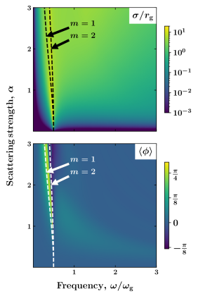
Figure 3: Scattering strength and frequency dependence of the total cross-section $\sigma$ (top) and average scattering angle $\langle\phi\rangle$ (bottom). The total cross-section is colored in a log scale, and the first two resonant harmonics $(m=1,2)$ are superimposed.

Fig. 2 presents the angular distribution of the plasma wave scattering evaluated via the partial wave analysis (left column) and perturbation theory (middle column). The high-frequency results exhibit slightly visible oscillations (they become more prominent at smaller $\alpha$ or even higher frequencies), which approximately follow the squared Fourier transform of the cyclotron frequency profile $|\omega_{\mathrm{c}}(\mathbf{k}-\mathbf{k}^{\prime})|^{2}$. Although the perturbation theory is expected to be reliable only in the weak-coupling regime $\alpha\ll 1$, it captures the high-frequency behavior reasonably well, even at $\alpha\sim 1$. In contrast, the perturbation theory completely fails to capture a prominent peak at low frequencies $\omega\lesssim\omega_{\mathrm{g}}/2$, which signals resonant plasma wave scattering. Before addressing its physical origin, we discuss the other scattering observables.

The angular distribution of the scattering of Dirac spin-1/2 electrons with the same disk-like Dirac mass profile is also presented in Fig. 2 (right column). The electronic scattering is also enhanced at low frequencies, but the dependence is smooth and resonance-free, showing a drastic difference from plasma wave scattering. In contrast, the high-frequency behavior appears almost indistinguishable; for this reason, this setup can be viewed as a classical simulator of Dirac electron scattering.

The dependence’s of the total cross-section $\sigma$ and average scattering angle $\langle\phi\rangle$ on the frequency of the incoming plasma wave $\omega/\omega_{\mathrm{g}}$ and the dimensionless parameter $\alpha$ are presented in Fig. 3. The frequency dependence of the total cross-section $\sigma$ has a narrow peak at the resonance frequency. The average scattering angle achieves a maximum below the resonance, rapidly switches its sign across the resonance, and then has a prominent minimum. The magnitude of the extrema (approximately $\pi/4$ and $-\pi/8$, respectively) drastically exceeds the typical average angle for electron scattering in nanostructures. Still, it is comparable to that for Dirac spin-1/2 electrons.

Resonant scattering and chiral interface modes. The presence of resonance is, perhaps, surprising. Magnetic fields tend to open the local gap in plasma wave dispersion and, therefore, act in a repulsive manner. Localized plasma waves, however, can be trapped at edges or different interfaces Sokolik et al. (2021); Mikhailov and Volkov (1992); Aleiner and Glazman (1994); Xia and Quinn (1994); Hasdeo and Song (2017); Ciobanu et al. (2022); Sun et al. (2023); Smith et al. (2019). Here, we argue that the plasma waves are not only trapped at the interface where the magnetic field vanishes but also circulate the micromagnet in only one direction.

The resonant nature of the scattering can be tracked in the frequency behavior of the S-matrix $S_{m}(\omega)=e^{2i\delta_{m}(\omega/\omega_{\mathrm{g}})}$ extended to the complex plane as $\omega=\omega^{\prime}+i\omega^{\prime\prime}$. Resonant modes manifest as poles below the real axis. As shown in the SM, $S_{m}(\omega)$ has a single pole for partial waves with $m\geq 1$. Furthermore, the number of resonant modes $n_{\mathrm{b}}$ can be determined according to

$$n_{\mathrm{b}}=\frac{\delta_{m}(0)-\delta_{m}(\infty)}{\pi},\quad n_{\mathrm{b}}=\begin{cases}1,&m\geq 1,\\ 0,&m<1,\end{cases}$$ (8)

which constitutes a heuristic proof of Levinson’s theorem Newton (1982). Because the bound modes appear only for positive $m$, they correspond to chiral waves circulating the gate in only one direction.

To further confirm this picture, it is instructive to shift from the disc geometry to a half-plane geometry, i.e., $\omega_{\mathrm{c}}(x)=\omega_{\mathrm{g}}\Theta(x)$. This interface supports a single chiral trapped mode with the following dispersion relation:

$$\Omega_{\text{int}}(k_{y})=\frac{uk_{y}\ \omega_{\mathrm{g}}}{\sqrt{4(uk_{y})^{2}+\omega_{\mathrm{g}}^{2}}}.$$ (9)

As presented in Fig. 4, the frequency of this mode is below the continua of bulk modes at both sides of the interface (red and blue shaded areas) and saturates towards $\omega=\omega_{\mathrm{g}}/2$. In the disc geometry, the standing wave condition $2\pi k_{m}r_{\mathrm{g}}=2\pi m$ results in discretization of the trapped mode wavevector. Therefore, the resonant frequencies can be approximated as $\Omega_{m}=\Omega_{\text{int}}(k_{m})$ and can be presented as $\Omega_{m}=\omega_{\mathrm{g}}/\sqrt{(\alpha/m)^{2}+4}$. Superimposed in Fig. 3, these frequencies accurately indicate the position of the scattering resonance, confirming that it originates from the the chiral trapped mode.

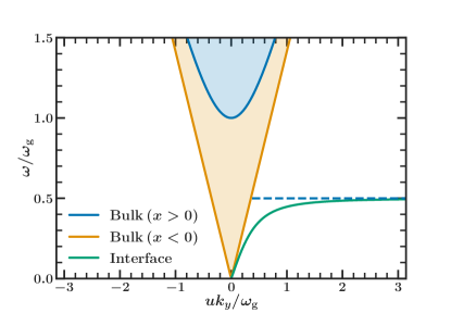
Figure 4: Dispersion of an interface plasma wave (green) localized at a magnetic field interface, i.e., $\omega_{\mathrm{c}}(x)=\omega_{\mathrm{g}}\Theta(x)$ and given by Eq. (9). Its frequency is below the continua of bulk states at both sides of the interface (orange and blue shaded areas). The edge mode propagates in only one direction and is, therefore, chiral.

Discussion: Plasma waves supported by a two-dimensional electron gas have been reported in various physical systems, including a liquid helium surface  Glattli et al. (1985); Mast et al. (1985), silicon inversion layers Allen et al. (1977), graphene Fei et al. (2012); Chen et al. (2012); Grigorenko et al. (2012), and other two-dimensional materials Scholz et al. (2013); Lian et al. (2020). In the considered setup, the monolayer graphene provides a few advantages. First, plasma waves have been reported there for a wide range of operating frequencies, spanning from mid-infrared to the terahertz range. Second, the extremely long relaxation times of monolayer graphene favor micrometer-sized plasma wave propagation. Third, the gated geometry (e.g., graphene-$\hbox{SiO}_{2}$-Si) is commonly used and permits electrical tuning of the plasma wave dispersion and cyclotron frequency. The latter is possible because the cyclotron mass $m$ for relativistic-like electrons with linear dispersion $\epsilon_{\mathbf{p}}=vp$ is doping-dependent $m=\sqrt{n\pi\hbar^{2}}/v$ and is not protected by Kohn’s theorem Kohn (1961). Regarding the micrometer-sized magnet, conventional magnets such as Ni, NiFe, and NiCr have been used in similar setups Aladyshkin et al. (2009); Ye et al. (1995); Jardine et al. (2021); Engdahl et al. (2022); Moshchalkov et al. (2006) and have been reported to produce magnetic fields up to a few dozen mT.

For estimations, we use the following set of parameters: electron velocity $v\approx 10^{8}\;\hbox{cm}/\hbox{s}$, electron concentration $n\approx 5\times 10^{11}\;\hbox{cm}^{-2}$, distance to the gate $d\approx 12\;\hbox{nm}$, effective dielectric constant for $\hbox{SiO}_{2}$ spacer $\kappa\approx 4$, magnetic field $B_{\mathrm{g}}\approx 30\;\hbox{mT}$, and micromagnet radius $r_{\mathrm{g}}\approx 3\;\mu\hbox{m}$. The smallness of the cyclotron mass $m\approx 0.15\;m_{0}$ enhances the magnetic field effect at plasma waves. Here, $m_{0}$ is the free electron mass. The other parameters of the model are $u\approx 1.3\times 10^{8}\;\hbox{cm/s}$ and $\omega_{\mathrm{g}}\approx 0.4\;\hbox{THz}$, resulting in moderate-strength scattering $\alpha=0.8$. The cyclotron frequency is in the infrared range, where plasma waves in graphene have been previously reported Grigorenko et al. (2012).

In recent years, it has been found that the spin-1 Dirac model describes a diverse family of platforms, including photonic metamaterials Zhu et al. (2017); Van Mechelen and Jacob (2018), superconducting qutrit circuits Tan et al. (2018), optical lattices in cold atomic setups Bercioux et al. (2009); Chen et al. (2019), and two-dimensional electronic systems with the $\alpha$-$T_{3}$ lattices, including $\hbox{SrTiO}_{3}$-$\hbox{SrIrO}_{3}$-$\hbox{SrTiO}_{3}$ trilayer heterostructures Wang and Ran (2011), $\hbox{so-MoS}_{2}$ allotropes Li et al. (2014), and graphene-$\hbox{In}_{2}\hbox{Te}_{2}$ bilayers Giovannetti et al. (2015). The Dirac mass term corresponds to a staggered sublattice potential and can be induced via substrate engineering. Thus, the predicted giant and resonant skew scattering can be potentially engineered in these systems, resulting in enhanced and tunable AHE.

In the considered setup, the magnetic field affects plasma waves via the local Hall conductivity. In graphene, the anomalous Hall response can be achieved via pumping with intensive circularly polarized light Kumar et al. (2016). Uniform pumping modifies the plasma wave dynamics and introduces non-reciprocity to the dispersion of edge plasma waves Song and Rudner (2016); Petrov (2021); Kumar et al. (2016). The plasma wave scattering off a non-uniform Hall response induced by a micrometer-sized light beam is also expected to be skewed, but a detailed theory is postponed for future studies.

To conclude, we predict giant and resonant plasma wave scattering off an adjacent micromagnet. The micrometer scale of the proposed setup can enable direct probes of individual skew scattering events previously inaccessible in electronic systems. The possibility of engineering the scattering target via the micromagnet shape (e.g., microring-shaped magnets) and/or external magnetic field opens further opportunities for classical simulations of quantum Dirac electron scattering.

Acknowledgments: We acknowledge fruitful discussions with Dimi Culcer, and Oleg Sushkov and support from the Australian Research Council Centre of Excellence in Future Low-Energy Electronics Technologies (CE170100039).

I The spin-1 reformulation

This section discusses the reformulation of the coupled hydrodynamic and Poisson equations as the spin-1 Dirac equation. The propagating charge density oscillations $\rho\left(\mathbf{r},t\right)$ induce the potential $\phi(\mathbf{r},t)$ which is given by

$$\phi(\mathbf{r},t)=\int d\mathbf{r}^{\prime}V\left(\mathbf{r}-\mathbf{r}^{\prime}\right)\rho\left(\mathbf{r}^{\prime},t\right),\;\;V(\mathbf{k})=\frac{2\pi}{k\kappa(\mathbf{k})}.$$ (S1)

The potential $V(\mathbf{q})$ incorporates the screening by the external media as $\kappa(\mathbf{k})=\kappa/\tanh(kd)$ Fetter (1985). Here $d$ is the distance to the gate, and $\kappa$ is the dielectric constant of the spacer. It is instructive to perform the Fourier transform, introduce the spinor $\psi(\mathbf{k},\omega)=\left\{j^{+}(\mathbf{k},\omega),j^{0}(\mathbf{k},\omega),j^{-}(\mathbf{k},\omega)\right\}$ with components $j^{\pm}(\mathbf{k},\omega)=\frac{1}{\sqrt{2}}\left[j^{x}(\mathbf{k},\omega)\pm ij^{y}(\mathbf{k},\omega)\right]$ and rescale the electronic density as $j^{0}(\mathbf{k},\omega)=\omega_{\mathrm{p}}(\mathbf{k})\rho(\mathbf{k},\omega)/k$. Here $\omega_{p}(\mathbf{k})=\sqrt{2\pi ne^{2}k\tanh(kd)/m\kappa}$ is the dispersion relation for magnetic field-free plasmons, which interpolates from the linear to the square-root dependence. The resulting equations can be presented as an eigenvalue problem $\omega\psi(\mathbf{k},\omega)=\hat{H}(\mathbf{k})\psi(\mathbf{k},\omega)$. The Hermitian $3\times 3$ matrix can be interpreted as the effective Hamiltonian of the system and is given by

$$\hat{H}(\mathbf{k})=\left(\begin{array}[]{ccc}\omega_{c}&\frac{\omega_{\mathrm{p}}(\mathbf{k})e^{i\phi_{\mathbf{k}}}}{\sqrt{2}}&0\\ \frac{\omega_{\mathrm{p}}(\mathbf{k})e^{-i\phi_{\mathrm{k}}}}{\sqrt{2}}&0&\frac{\omega_{\mathrm{p}}(\mathbf{k})e^{i\phi_{\mathbf{k}}}}{\sqrt{2}}\\ 0&\frac{\omega_{\mathrm{p}}(\mathbf{k})e^{-i\phi_{\mathbf{k}}}}{\sqrt{2}}&-\omega_{c}.\end{array}\right).$$ (S2)

Its eigenvalues have the three branches

$$\Omega^{\pm}(\mathbf{k})=\pm\Omega(\mathbf{k})\quad\text{ and }\quad\Omega^{0}(\mathbf{k})=0.$$ (S3)

The positive frequency branch $\Omega(\mathbf{k})=\sqrt{\omega^{2}_{\mathrm{c}}+\omega_{\mathrm{p}}^{2}(\mathbf{k})}$ governs the dynamics for plasma waves, and is gapped by the Larmor frequency. The negative-frequency branch is connected to the positive branch by the particle-hole symmetry transformation and is not dynamically independent. The zero-frequency branch is spurious, and its flatness is protected by the interplay of inversion $\left[\Omega^{0}(\mathbf{k})=\Omega^{0}(-\mathbf{k})\right]$ and the particle-hole $\left[\Omega^{0}(-\mathbf{k})=-\Omega^{0}(\mathbf{k})\right]$ symmetries. If we approximate the dispersion of plasma waves by its long-wavelength linear behavior $\omega_{\mathrm{p}}=uk$, the Hamiltonian reduces to the spin-1 Dirac model presented as Eq. (2) in the main text of the Letter.

II The scattering phase shifts

This section presents the derivation of scattering phase shifts for plasma waves. Due to the azimuthal symmetry of the magnetic field, it is natural to use the polar coordinates $\mathbf{r}=(r,\phi)$ and present the wave function for each angular harmonics $m$ as

$$\psi_{m}(r,\phi,\omega)=\begin{pmatrix}\psi^{+}(r,\omega)e^{i(m-1)\phi}\\ \psi^{0}(r,\omega)e^{im\phi}\\ \psi^{-}(r,\omega)e^{i(m+1)\phi}\end{pmatrix}.$$ (S4)

The top and the bottom components of the spinor can be presented as

$$\psi^{+}(r,\omega)=\frac{-iu}{\sqrt{2}\left[\omega-\omega_{c}(\mathbf{r})\right]}\left(\partial_{r}+\frac{m}{r}\right)\psi^{0}(r,\omega),$$ (S5)

$$\psi^{-}(r,\omega)=\frac{-iu}{\sqrt{2}\left[\omega+\omega_{c}(\mathbf{r})\right]}\left(\partial_{r}-\frac{m}{r}\right)\psi^{0}(r,\omega),$$ (S6)

and its central component $\psi^{0}(r,\omega)$ satisfies the closed equation as

$$\kappa^{2}(\mathbf{r})\psi^{0}(r,\omega)-\left(\partial_{r}^{2}+\frac{1}{r}\partial_{r}-\frac{m^{2}}{r^{2}}\right)\psi^{0}(r,\omega)=0.$$ (S7)

Here we have introduced $\kappa(\mathbf{r})=\sqrt{|\omega^{2}-\omega_{c}(\mathbf{r})^{2}|}/u$. It is instructive to consider the inner ($r<r_{\mathrm{g}}$) and outer ($r>r_{\mathrm{g}}$) regions separately. They will be labeled as I and II, respectively. In the outer region, the wave function can be presented as

$$\psi^{\mathrm{II}}_{m}=B_{m}\begin{pmatrix}-iJ_{m-1}(kr)\\ J_{m}(kr)\\ iJ_{m+1}(kr)\end{pmatrix}+C_{m}\begin{pmatrix}-iY_{m-1}(kr)\\ Y_{m}(kr)\\ iY_{m+1}(kr)\end{pmatrix}.$$ (S8)

Here $k=\omega/u$ is the wavevector magnitude for the incoming plasma wave; $J_{m}$ and $Y_{m}$ are the Bessel functions of the first and the second kind. The wave function Eq. (S8) has oscillatory behavior, and its asymptotics differs from the one for the free plasma wave (in the absence of the micromagnet) only by the phase shift $\delta_{m}=\arctan\left(C_{m}/B_{m}\right)$. In contrast, the behavior of the wave function in the inner region depends on the relation between the frequency of incoming plasma wave $\omega$ and the local Larmor frequency $\omega_{\mathrm{g}}$ induced by the ferromagnetic gate. If $\omega>\omega_{\mathrm{g}}$, the wave function is also oscillatory and is given by

$$\psi_{m}^{\mathrm{I}}=A_{m}\begin{pmatrix}\frac{-i}{\sqrt{2}}\sqrt{\frac{\omega+\omega_{\mathrm{g}}}{\omega-\omega_{\mathrm{g}}}}J_{m-1}(\kappa r)\\ J_{m}(\kappa r)\\ \frac{i}{\sqrt{2}}\sqrt{\frac{\omega-\omega_{\mathrm{g}}}{\omega+\omega_{\mathrm{g}}}}J_{m+1}(\kappa r)\end{pmatrix}.$$ (S9)

If $\omega<\omega_{g}$, the wave function is evanescent and decays toward the center of ferromagnet as

$$\psi_{m}^{\mathrm{I}}=A_{m}\begin{pmatrix}\frac{i}{\sqrt{2}}\sqrt{\frac{\omega_{\mathrm{g}}+\omega}{\omega_{\mathrm{g}}-\omega}}I_{m-1}(\kappa r)\\ I_{m}(\kappa r)\\ \frac{-i}{\sqrt{2}}\sqrt{\frac{\omega_{\mathrm{g}}-\omega}{\omega_{\mathrm{g}}+\omega}}I_{m+1}(\kappa r)\end{pmatrix}.$$ (S10)

Here $I_{m}$ is the modified Bessel function of the first kind.

To coefficients $A_{m}$, $B_{m}$ and $C_{m}$ can be found using boundary conditions at the interface. First, the continuity of the scalar potential dictates

$$\psi_{m}^{0,\mathrm{I}}(r_{\mathrm{g}}) =\psi_{m}^{0,\mathrm{II}}(r_{\mathrm{g}}),$$ (S11)

Second, charge conservation dictates the radial component of electric current density to be continuous across the interface, which implies

$$\psi_{m}^{+,\mathrm{I}}(r_{\mathrm{g}})+\psi_{m}^{-,\mathrm{I}}(r_{\mathrm{g}})=\psi_{m}^{+,\mathrm{II}}(r_{\mathrm{g}})+\psi_{m}^{-,\mathrm{II}}(r_{\mathrm{g}}),$$ (S12)

As for the azimuthal component of the electric current density, it can be discontinuous across the interface. These two boundary conditions are sufficient (all three of them can be calculated if we add the normalization condition for the wave function) to calculate the ratios $B_{m}/A_{m}$ and $C_{m}/A_{m}$, which determine plasma waves phase shifts as $\delta_{m}=\arctan\left(C_{m}/B_{m}\right)$. The explicit calculations result in

$$\left(\frac{B_{m}}{A_{m}}\right)_{\omega<\omega_{\mathrm{g}}}=\frac{Y_{m}(kr_{\mathrm{g}})\left(\sqrt{\frac{\omega+\text{$\omega_{\mathrm{g}}$}}{\text{$\omega_{\mathrm{g}}$}-\omega}}I_{m-1}(\kappa r_{\mathrm{g}})-\sqrt{\frac{\text{$\omega_{\mathrm{g}}$}-\omega}{\omega+\text{$\omega_{\mathrm{g}}$}}}I_{m+1}(\kappa r_{\mathrm{g}})\right)+(Y_{m-1}(kr_{\mathrm{g}})-Y_{m+1}(kr_{\mathrm{g}}))I_{m}(\kappa r_{\mathrm{g}})}{(J_{m+1}(kr_{\mathrm{g}})-J_{m-1}(kr_{\mathrm{g}}))Y_{m}(kr_{\mathrm{g}})+J_{m}(kr_{\mathrm{g}})(Y_{m-1}(kr_{\mathrm{g}})-Y_{m+1}(kr_{\mathrm{g}}))},$$ (S13)

$$\left(\frac{C_{m}}{A_{m}}\right)_{\omega<\omega_{\mathrm{g}}}=\frac{J_{m}(kr_{\mathrm{g}})\left(\sqrt{\frac{\omega+\text{$\omega_{\mathrm{g}}$}}{\text{$\omega_{\mathrm{g}}$}-\omega}}I_{m-1}(\kappa r_{\mathrm{g}})-\sqrt{\frac{\text{$\omega_{\mathrm{g}}$}-\omega}{\omega+\text{$\omega_{\mathrm{g}}$}}}I_{m+1}(\kappa r_{\mathrm{g}})\right)+(J_{m-1}(kr_{\mathrm{g}})-J_{m+1}(kr_{\mathrm{g}}))I_{m}(\kappa r_{\mathrm{g}})}{(J_{m-1}(kr_{\mathrm{g}})-J_{m+1}(kr_{\mathrm{g}}))Y_{m}(kr_{\mathrm{g}})+J_{m}(kr_{\mathrm{g}})(Y_{m+1}(kr_{\mathrm{g}})-Y_{m-1}(kr_{\mathrm{g}}))},$$

                                                                         and

$$\left(\frac{B_{m}}{A_{m}}\right)_{\omega>\omega_{\mathrm{g}}}=\frac{-Y_{m}(kr_{\mathrm{g}})\left(\sqrt{\frac{\omega+\text{$\omega_{\mathrm{g}}$}}{\omega-\text{$\omega_{\mathrm{g}}$}}}J_{m-1}(\kappa r_{\mathrm{g}})-\sqrt{\frac{\omega-\text{$\omega_{\mathrm{g}}$}}{\omega+\text{$\omega_{\mathrm{g}}$}}}J_{m+1}(\kappa r_{\mathrm{g}})\right)+(Y_{m-1}(kr_{\mathrm{g}})-Y_{m+1}(kr_{\mathrm{g}}))J_{m}(\kappa r_{\mathrm{g}})}{(J_{m+1}(kr_{\mathrm{g}})-J_{m-1}(kr_{\mathrm{g}}))Y_{m}(kr_{\mathrm{g}})+J_{m}(kr_{\mathrm{g}})(Y_{m-1}(kr_{\mathrm{g}})-Y_{m+1}(kr_{\mathrm{g}}))},$$ (S14)

$$\left(\frac{C_{m}}{A_{m}}\right)_{\omega>\omega_{\mathrm{g}}}=\frac{-J_{m}(kr_{\mathrm{g}})\left(\sqrt{\frac{\omega+\omega_{\mathrm{g}}}{\omega-\omega_{\mathrm{g}}}}J_{m-1}(\kappa r_{\mathrm{g}})+\sqrt{\frac{\omega-\omega_{\mathrm{g}}}{\omega+\omega_{\mathrm{g}}}}J_{m+1}(\kappa r_{\mathrm{g}})\right)+\left(Y_{m-1}(kr_{\mathrm{g}})-Y_{m+1}(kr_{\mathrm{g}})\right)J_{m}(\kappa r_{\mathrm{g}})}{(J_{m-1}(kr_{\mathrm{g}})-J_{m+1}(kr_{\mathrm{g}}))Y_{m}(kr_{\mathrm{g}})+J_{m}(kr_{\mathrm{g}})(Y_{m+1}(kr_{\mathrm{g}})-Y_{m-1}(kr_{\mathrm{g}}))}.$$

The corresponding phase shifts have been used to calculate the scattering observables, which are presented in the main text of the paper.

III Perturbative scattering theory

This section provides details on the derivation of Eq. (4) in the main part of the Letter. The differential cross-section for the plasma wave scattering

$$\frac{d\sigma}{d\phi}=\frac{k}{2\pi u^{2}}\cdot|T_{\mathbf{k}^{\prime}\mathbf{k}}(\Omega_{\mathbf{k}})|^{2}.$$ (S15)

is determined by the T-matrix, which in the second-order Born approximation is approximated as $\hat{T}_{\mathbf{k}^{\prime}\mathbf{k}}(\omega)=\hat{V}_{\mathbf{k}^{\prime}\mathbf{k}}+\sum_{\mathbf{k}^{\prime\prime}}\hat{V}_{\mathbf{k}^{\prime}\mathbf{k}^{\prime\prime}}\hat{G}(\omega,\mathbf{k}^{\prime\prime})\hat{V}_{\mathbf{k}^{\prime\prime}\mathbf{k}}$. Here $G(\omega,\mathbf{k})=(\omega-\hat{H}(\mathbf{k})+i\epsilon)^{-1}$ is the Green function for the effective Hamiltonian $\hat{H}(\mathbf{k})$ describing the plasma waves. Up to third order in the potential $\hat{V}$, the differential cross section is given by

$$\begin{split}\frac{d\sigma}{d\phi}\approx\frac{k}{2\pi u^{2}}\Big{(}|\hat{V}_{\mathbf{k}^{\prime}\mathbf{k}}|^{2}+2\sum_{k^{\prime\prime}}\mathop{\mathrm{Re}}\nolimits\big{[}\hat{V}_{\mathbf{k}^{\prime}\mathbf{k}^{\prime\prime}}\hat{V}_{\mathbf{k}^{\prime\prime}\mathbf{k}}\hat{V}_{\mathbf{k}\mathbf{k}^{\prime}}\big{]}\times\\ G^{\prime}(\Omega_{\mathbf{k}},\mathbf{k}^{\prime\prime})-2\sum_{\mathbf{k}^{\prime\prime}}\mathop{\mathrm{Im}}\nolimits\big{[}\hat{V}_{\mathbf{k}^{\prime}\mathbf{k}^{\prime\prime}}\hat{V}_{\mathbf{k}^{\prime\prime}\mathbf{k}}\hat{V}_{\mathbf{k}\mathbf{k}^{\prime}}\big{]}G^{\prime\prime}(\Omega_{\mathbf{k}},\mathbf{k}^{\prime\prime})\Big{)}.\end{split}$$

Here $G^{\prime}(\omega,\mathbf{k})$ and $G^{\prime\prime}(\omega,\mathbf{k})$ are real and imaginary parts of the Green function. The explicit calulation of the matrix element $\hat{V}_{\mathbf{k}\mathbf{k}^{\prime}}=i\pi r_{\mathrm{g}}\omega_{\mathrm{g}}J_{1}(kr_{\mathrm{g}})\sin(\phi_{\mathbf{k}}-\phi_{\mathbf{k}}^{\prime})/k$ demonstrates that it has only the imaginary part and the second term in the equation above vanishes. If we incorporate the explicit expression for the imaginary part of the Green function $G^{\prime\prime}(\Omega_{\mathbf{k}},\mathbf{k}^{\prime\prime})=-\pi\delta(\Omega_{\mathbf{k}^{\prime\prime}}-\Omega_{\mathbf{k}})$, the resulting expression for the cross-section matches with Eq. (4) presented in the main part of the Letter.

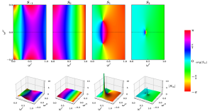
Figure 1: S-matrix plotted in the complex plane for harmonics $m=-1,0,1,2$. Shown in the top row are complex phase plots for each S-matrix harmonic, as labeled, and in the bottom row we present the same data but with the magnitude of the complex S-matrix projected on the z-axis.

IV Poles of the S-matrix

The resonant nature of the scattering can be tracked in the frequency behavior of the S-matrix $S_{m}(\omega)=e^{2i\delta_{m}(\omega/\omega_{\mathrm{g}})}$ extended to the complex plane as $\omega=\omega^{\prime}+i\omega^{\prime\prime}$. The corresponding frequency dependence for orbital numbers $m=-1,0,1,2$ is presented in Fig. (1). The resonances manifest as poles in the lower part of the complex plane. Notably, a single pole for partial waves with $m\geq 1$ exists. In contrast, the partial waves with $m\leq 0$ are free of any poles in the complex plane. This behavior demonstrates that the presence of the resonant plasma wave scattering is due to the trapped chiral mode circulating the micromagnet.

V Extra metallic screening by the micromagnet

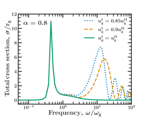
Figure 2: Frequency dependence of total cross section, $\sigma$, when the plasma wave velocity is equal across interface (green) and when the velocity is altered mismatched by $u_{\mathrm{g}}^{\mathrm{I}}=0.85u_{\mathrm{g}}^{\mathrm{II}}$ (blue, dotted) and $u_{\mathrm{g}}^{\mathrm{I}}=0.9u_{\mathrm{g}}^{\mathrm{II}}$ (orange, dashed). Calculated for scattering strength $\alpha$ as labeled.

The micrometer-sized magnets Ni, NiFe, and NiCr used in similar setups Aladyshkin et al. (2009); Ye et al. (1995); Jardine et al. (2021); Engdahl et al. (2022); Moshchalkov et al. (2006) are metallic and provide additional screening. The additional screening under the micromagnet reduces the plasma wave velocity as $u_{\mathrm{g}}=u\sqrt{d_{\mathrm{g}}/(d+d_{\mathrm{g}})}$, where $d_{\mathrm{g}}$ is the distance to the micromagnet. Since the velocity of plasma waves manifests itself explicitly in the expression for the spinor $\psi(\mathbf{r},t)=\left[j_{+}(\mathbf{r},t),u\rho(\mathbf{r},t),j_{-}(\mathbf{r},t)\right]$ the boundary condition which ensures the continuity of the electric potential needs to be modified as follows

$$\frac{1}{u_{\mathrm{g}}^{\mathrm{I}}}\psi_{m}^{0,\mathrm{I}}(r_{\mathrm{g}})=\frac{1}{u_{\mathrm{g}}^{\mathrm{II}}}\psi_{m}^{0,\mathrm{II}}(r_{\mathrm{g}}),$$ (S16)

Here $u_{\mathrm{g}}^{\mathrm{I}(\mathrm{II})}$ are plasma wave velocities at both sides of the interface. Otherwise, the calculation of the phase shifts $\delta_{m}(\mathbf{k})$ follows the same steps, which are presented in Sec. II.

For calculations, we chose the spacing between graphene and the micromagnet as $d_{\mathrm{g}}=50\;\hbox{nm}$ and $d_{\mathrm{g}}=30\;\hbox{nm}$. As a result, plasma wave velocity below the micromagnet is reduced as $u_{\mathrm{g}}^{\mathrm{I}}\approx 0.9u_{\mathrm{g}}^{\mathrm{II}}$ and $u_{\mathrm{g}}^{\mathrm{I}}\approx 0.85u_{\mathrm{g}}^{\mathrm{II}}$, respectively. The corresponding frequency dependence of the total cross-section for the plasma waves scattering (supplemented by the curve for $u_{\mathrm{g}}^{\mathrm{II}}=u_{\mathrm{g}}^{\mathrm{I}}$, which corresponds to the absence of the additional screening) is presented in Fig. (2). The oscillations we see at high frequencies in Fig. (2) are due solely to the additional screening introduced via the micromagnet, and the scattering in this region is not skewed. Furthermore, it is seen that the resonance is completely robust to the additional screening, as in the low-frequency region the contribution to the scattering amplitudes is dominated by the resonant skew scattering due to the chiral interface mode.

VI The high-frequency behavior for electron and plasma wave scattering

In the main text of the Letter, we showed that the low-frequency ($\omega\lesssim\omega_{\mathrm{g}}$) scattering of plasma waves and Dirac electrons are drastically different. Here, we demonstrate that their high-frequency ($\omega\gg\omega_{\mathrm{g}}$) behaviors are very close to each other. The corresponding angular and frequency dependence of the differential cross-section $d\sigma/d\phi$ is presented in Fig. 3. We note that although the magnitude of fine oscillations is slightly different for the two problems, the corresponding dependencies still match quite well for both considered scattering strength $\alpha=0.8$ and $\alpha=1.6$.

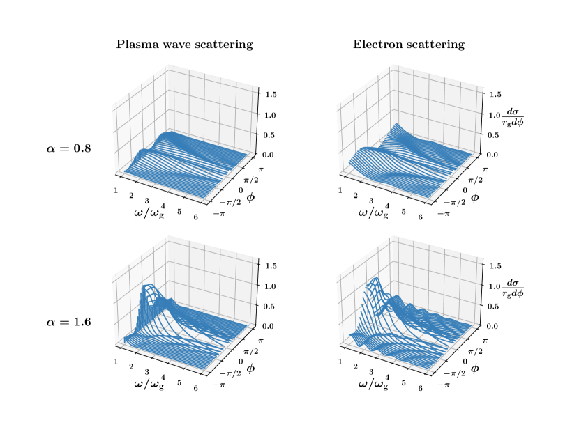
Figure 3: Angular and frequency dependence of the differential cross-section $d\sigma/d\phi$ in a high frequency ($\omega_{\mathrm{g}}\leq\omega\leq 6\omega_{\mathrm{g}}$) regime for the scattering of plasma waves (left column) and the scattering of electrons (right column). Scattering strengths, $\alpha$, are as labeled.

References

- Hasan and Kane (2010) M. Z. Hasan and C. L. Kane, Rev. Mod. Phys. 82, 3045 (2010).
- Hasan and Moore (2011) M. Z. Hasan and J. E. Moore, Annual Review of Condensed Matter Physics 2, 55 (2011).
- Burkov and Hawthorn (2010) A. A. Burkov and D. G. Hawthorn, Phys. Rev. Lett. 105, 066802 (2010).
- Garate and Franz (2010) I. Garate and M. Franz, Phys. Rev. Lett. 104, 146802 (2010).
- Hurst et al. (2015) H. M. Hurst, D. K. Efimkin, J. Zang, and V. Galitski, Phys. Rev. B 91, 060401 (2015).
- Divic et al. (2022) S. Divic, H. Ling, T. Pereg-Barnea, and A. Paramekanti, Phys. Rev. B 105, 035156 (2022).
- Paul and Fu (2021) N. Paul and L. Fu, Phys. Rev. Res. 3, 033173 (2021).
- Kurebayashi and Nagaosa (2019) D. Kurebayashi and N. Nagaosa, Phys. Rev. B 100, 134407 (2019).
- Efimkin and Kargarian (2021) D. K. Efimkin and M. Kargarian, Phys. Rev. B 104, 075413 (2021).
- Kargarian et al. (2016) M. Kargarian, D. K. Efimkin, and V. Galitski, Phys. Rev. Lett. 117, 076806 (2016).
- Martinez-Berumen et al. (2023) I. Martinez-Berumen, W. A. Coish, and T. Pereg-Barnea, Phys. Rev. B 107, 205110 (2023).
- Bhattacharyya et al. (2021) S. Bhattacharyya, G. Akhgar, M. Gebert, J. Karel, M. T. Edmonds, and M. S. Fuhrer, Advanced Materials 33, 2170262 (2021).
- Hirohata et al. (2020) A. Hirohata, K. Yamada, Y. Nakatani, I.-L. Prejbeanu, B. Dieny, P. Pirro, and B. Hillebrands, Journal of Magnetism and Magnetic Materials 509, 166711 (2020).
- Nagaosa et al. (2010) N. Nagaosa, J. Sinova, S. Onoda, A. H. MacDonald, and N. P. Ong, Rev. Mod. Phys. 82, 1539 (2010).
- Culcer and Das Sarma (2011) D. Culcer and S. Das Sarma, Phys. Rev. B 83, 245441 (2011).
- Sabzalipour and Partoens (2019) A. Sabzalipour and B. Partoens, Phys. Rev. B 100, 035419 (2019).
- Liu et al. (2018) N. Liu, J. Teng, and Y. Li, Nature Communications 9, 1282 (2018).
- Culcer et al. (2020) D. Culcer, A. Cem Keser, Y. Li, and G. Tkachov, 2D Materials 7, 022007 (2020).
- Jin et al. (2016) D. Jin, L. Lu, Z. Wang, C. Fang, J. D. Joannopoulos, M. Soljačić, L. Fu, and N. X. Fang, Nature Communications 7, 13486 (2016).
- Fetter (1985) A. L. Fetter, Phys. Rev. B 32, 7676 (1985).
- Finnigan et al. (2022) C. Finnigan, M. Kargarian, and D. K. Efimkin, Phys. Rev. B 105, 205426 (2022).
- Ciobanu et al. (2022) A. Ciobanu, P. Cosme, and H. Tercas, “Topological waves in the continuum in magnetized graphene devices,” (2022), arXiv:2212.01489 [cond-mat.mes-hall] .
- Sun et al. (2023) W. Sun, T. V. Mechelen, S. Bharadwaj, A. K. Boddeti, and Z. Jacob, New Journal of Physics 25, 113009 (2023).
- Van Mechelen et al. (2021) T. Van Mechelen, W. Sun, and Z. Jacob, Nature Communications 12, 4729 (2021).
- Grigorenko et al. (2012) A. N. Grigorenko, M. Polini, and K. S. Novoselov, Nature Photonics 6, 749 (2012).
- Fei et al. (2012) Z. Fei, A. S. Rodin, G. O. Andreev, W. Bao, A. S. McLeod, M. Wagner, L. M. Zhang, Z. Zhao, M. Thiemens, G. Dominguez, M. M. Fogler, A. H. C. Neto, C. N. Lau, F. Keilmann, and D. N. Basov, Nature 487, 82 (2012).
- Chen et al. (2012) J. Chen, M. Badioli, P. Alonso-González, S. Thongrattanasiri, F. Huth, J. Osmond, M. Spasenović, A. Centeno, A. Pesquera, P. Godignon, A. Zurutuza Elorza, N. Camara, F. J. G. de Abajo, R. Hillenbrand, and F. H. L. Koppens, Nature 487, 77 (2012).
-
Note (1)
The symmetry works as . The explicit expression for is given by
where is the complex conjugation operator. Only the positive frequency states correspond to physical modes supported by two-dimensional electron gas. - Efimkin et al. (2012) D. K. Efimkin, Y. E. Lozovik, and A. A. Sokolik, Nanoscale Research Letters 7, 163 (2012).
- Torre et al. (2017) I. Torre, M. I. Katsnelson, A. Diaspro, V. Pellegrini, and M. Polini, Phys. Rev. B 96, 035433 (2017).
- Koskamp et al. (2023) T. M. Koskamp, M. I. Katsnelson, and K. J. A. Reijnders, Phys. Rev. B 108, 085414 (2023).
- Jiang et al. (2017) B.-Y. Jiang, G.-X. Ni, Z. Addison, J. K. Shi, X. Liu, S. Y. F. Zhao, P. Kim, E. J. Mele, D. N. Basov, and M. M. Fogler, Nano Letters 17, 7080 (2017).
- Zabolotnykh et al. (2021) A. A. Zabolotnykh, V. V. Enaldiev, and V. A. Volkov, Phys. Rev. B 104, 195435 (2021).
- Wolski et al. (2023) S. Wolski, V. K. Dugaev, and E. Y. Sherman, Phys. Rev. Res. 5, 023164 (2023).
- Araki and Nomura (2017) Y. Araki and K. Nomura, Phys. Rev. B 96, 165303 (2017).
- Wang et al. (2020) C.-Z. Wang, H.-Y. Xu, and Y.-C. Lai, Phys. Rev. Res. 2, 013247 (2020).
- Note (2) Supplementary material.
- Sokolik et al. (2021) A. A. Sokolik, O. V. Kotov, and Y. E. Lozovik, Phys. Rev. B 103, 155402 (2021).
- Mikhailov and Volkov (1992) S. A. Mikhailov and V. A. Volkov, Journal of Physics: Condensed Matter 4, 6523 (1992).
- Aleiner and Glazman (1994) I. L. Aleiner and L. I. Glazman, Phys. Rev. Lett. 72, 2935 (1994).
- Xia and Quinn (1994) X. Xia and J. J. Quinn, Phys. Rev. B 50, 11187 (1994).
- Hasdeo and Song (2017) E. H. Hasdeo and J. C. W. Song, Nano Letters 17, 7252 (2017).
- Smith et al. (2019) T. B. Smith, I. Torre, and A. Principi, Phys. Rev. B 99, 155422 (2019).
- Newton (1982) R. G. Newton, Scattering Theory of Waves and Particles (Springer Berlin Heidelberg, 1982).
- Glattli et al. (1985) D. C. Glattli, E. Y. Andrei, G. Deville, J. Poitrenaud, and F. I. B. Williams, Phys. Rev. Lett. 54, 1710 (1985).
- Mast et al. (1985) D. B. Mast, A. J. Dahm, and A. L. Fetter, Phys. Rev. Lett. 54, 1706 (1985).
- Allen et al. (1977) S. J. Allen, D. C. Tsui, and R. A. Logan, Phys. Rev. Lett. 38, 980 (1977).
- Scholz et al. (2013) A. Scholz, T. Stauber, and J. Schliemann, Phys. Rev. B 88, 035135 (2013).
- Lian et al. (2020) C. Lian, S.-Q. Hu, J. Zhang, C. Cheng, Z. Yuan, S. Gao, and S. Meng, Phys. Rev. Lett. 125, 116802 (2020).
- Kohn (1961) W. Kohn, Phys. Rev. 123, 1242 (1961).
- Aladyshkin et al. (2009) A. Y. Aladyshkin, A. V. Silhanek, W. Gillijns, and V. V. Moshchalkov, Superconductor Science and Technology 22, 053001 (2009).
- Ye et al. (1995) P. Ye, D. Weiss, K. Klitzing, K. Eberl, and H. Nickel, Applied Physics Letters 67, 1441 (1995).
- Jardine et al. (2021) M. J. A. Jardine, J. P. T. Stenger, Y. Jiang, E. J. de Jong, W. Wang, A. C. B. Jayich, and S. M. Frolov, SciPost Phys. 11, 090 (2021).
- Engdahl et al. (2022) J. N. Engdahl, A. i. e. i. f. C. Keser, and O. P. Sushkov, Phys. Rev. Res. 4, 043175 (2022).
- Moshchalkov et al. (2006) V. V. Moshchalkov, D. S. Golubovi~Ç, and M. Morelle, Comptes Rendus Physique 7, 86 (2006), superconductivity and magnetism.
- Zhu et al. (2017) Y.-Q. Zhu, D.-W. Zhang, H. Yan, D.-Y. Xing, and S.-L. Zhu, Phys. Rev. A 96, 033634 (2017).
- Van Mechelen and Jacob (2018) T. Van Mechelen and Z. Jacob, Phys. Rev. A 98, 023842 (2018).
- Tan et al. (2018) X. Tan, D.-W. Zhang, Q. Liu, G. Xue, H.-F. Yu, Y.-Q. Zhu, H. Yan, S.-L. Zhu, and Y. Yu, Phys. Rev. Lett. 120, 130503 (2018).
- Bercioux et al. (2009) D. Bercioux, D. F. Urban, H. Grabert, and W. Häusler, Physical Review A 80, 063603 (2009).
- Chen et al. (2019) Y.-R. Chen, Y. Xu, J. Wang, J.-F. Liu, and Z. Ma, Phys. Rev. B 99, 045420 (2019).
- Wang and Ran (2011) F. Wang and Y. Ran, Phys. Rev. B 84, 241103 (2011).
- Li et al. (2014) W. Li, M. Guo, G. Zhang, and Y.-W. Zhang, Phys. Rev. B 89, 205402 (2014).
- Giovannetti et al. (2015) G. Giovannetti, M. Capone, J. van den Brink, and C. Ortix, Phys. Rev. B 91, 121417 (2015).
- Kumar et al. (2016) A. Kumar, A. Nemilentsau, K. H. Fung, G. Hanson, N. X. Fang, and T. Low, Phys. Rev. B 93, 041413 (2016).
- Song and Rudner (2016) J. C. W. Song and M. S. Rudner, Proceedings of the National Academy of Sciences 113, 4658 (2016).
- Petrov (2021) A. S. Petrov, Phys. Rev. B 104, L241407 (2021).
Supplemental Material for