Distributed Finite-time Differentiator for Multi-agent Systems Under Directed Graph

Abstract

This paper proposes a new distributed finite-time differentiator (DFD) for multi-agent systems (MAS) under directed graph, which extends the differentiator algorithm from the centralized case to the distributed case by only using relative/absolute position information. By skillfully constructing a Lyapunov function, the finite-time stability of the closed-loop system under DFD is proved. Inspired by the duality principle of control theory, a distributed continuous finite-time output consensus algorithm extended from DFD for a class of leader-follower MAS is provided, which not only completely suppresses disturbance, but also avoids chattering. Finally, several simulation examples are given to verify the effectiveness of the DFD.

I Introduction

The differentiator means that for a real-time measurable signal $f(t)$, design an algorithm to estimate $\dot{f}(t)$ under certain conditions. Based on the second-order sliding mode algorithm, namely the super-twisting algorithm [1], a famous differentiator algorithm was proposed in [2]. Considering that many mechanical systems can be modeled by a second-order system, the super-twisting algorithm was employed to solve the control problem in [3]. For the high-order systems, the corresponding differentiator algorithm and output feedback control algorithm were introduced in [4]. In order to accelerate the convergence speed, uniformly convergent differentiators were proposed in [5, 6].

The above differentiator can be regarded as centralized differentiator. With the development of science and technology, networks are playing an increasingly important role [7]. In the early stage, in [8, 9], the asymptotical consensus of second-order leader-follower MAS was realized by designing distributed observers. The distributed observers for linear systems were studied in [7, 10, 11]. In [12], the cooperative output regulation of LTI plant was solved based on the distributed observer. Considering the uncertainty and disturbance of the system, robust distributed observers were proposed in [13, 14]. Combining with adaptive control method, adaptive distributed observers were proposed in [15, 16, 17]. In addition, distributed finite-time and fixed-time observers were proposed in [18, 19], respectively. However, most of these observers need the leader’s internal state information (equivalent to $\dot{f}(t)$) or control input information (equivalent to $\ddot{f}(t)$), so they are not distributed differentiators. To the best of our knowledge, no related algorithm can achieve the same function, i.e., distributed finite-time differentiator.

In the cooperative control of leader-follower MAS, the full states or partial internal states of leader are required in most works, which precludes many practical applications where only the output of the leader system is available [20]. In practice, sometimes only the relative position information can be obtained rather than the absolute global position, and for each follower agent, the more important information is the relative position and relative velocity between itself and the leader, rather than the absolute global position and absolute global velocity. For example, for groups of mobile robots, the global positions of the robots are usually not available while the relative position measurements should be used instead [21]. In addition, it is more difficult to get velocity and acceleration measurements than position measurement [22, 23] and the follower agents might not be equipped with velocity sensors to save space, cost and weight [25, 24]. Therefore, the study of distributed observer and controller based only on the relative position information has important theoretical significance and practical value [26].

The main contributions of this paper are given as follows. Firstly, unlike the centralized finite-time differentiator, a framework of distributed finite-time differentiator (DFD) is proposed, which can achieve the exact differential estimation only if the differentiable signal $f(t)$ is available for at least one agent. The distributed finite-time differentiator can be realized via the absolute position information or relative position information, which is more available for formation control without global position information. Secondly, the distributed finite-time differentiator is employed to design a new distributed finite-time consensus control algorithm, which can achieve finite-time output consensus of a class of leader-follower MAS under disturbance. Unlike the discontinuous consensus controllers [27, 28], the consensus controller proposed in this paper is continuous, which not only completely suppresses disturbance, but also avoids chattering.

Notations: For any vector ${\bf x}=[x_{1},x_{2},...,x_{n}]^{T}\in R^{n}$, we give some notations.
(1) $\lfloor x_{i}\rceil^{a}={\rm sgn}(x_{i})|x_{i}|^{a}$, $a\geq 0$. Especially, when $a=0$, define $\lfloor x_{i}\rceil^{0}={\rm sgn}(x_{i})$.
(2) ${\rm diag}({\bf x})\in R^{n\times n}$ indicates the diagonal matrix with the diagonal element of vector ${\bf x}$.
(3) $\lfloor{\bf x}\rceil^{a}=\Big{[}\lfloor x_{1}\rceil^{a},\lfloor x_{2}\rceil^{a},...,\lfloor x_{n}\rceil^{a}\Big{]}^{T}\in R^{n}$, $a\geq 0$.
(4) If matrix $Q=Q^{T}\in R^{n}$ is positive definite, it is recorded as $Q>0$, and the eigenvalues of matrix $Q$ are sorted by size, where the maximum and minimum values are recorded as $\lambda_{n}(Q)$ and $\lambda_{1}(Q)$ respectively.
(5) Denote ${\bf 1}=[1,...,1]^{T}$ and ${\bf 0}=[0,...,0]^{T}$ with appropriate dimension.

II Necessary preparation

II-A Graph theory

The directed graph is often used to describe the communication topology of MAS. $\Psi=\{V,E,A\}$ represents the connectivity among agents. $V=\{v_{i},i=1,\cdots,n\}$ is the set of vertices, $A=[a_{ij}]\in R^{n\times n}$ is the weighted adjacency matrix and $E\subseteq V\times V$ is the set of edges. Define $\Gamma=\{1,\cdots,n\}$ as node indexes. If $(v_{j},v_{i})\in E$, then $a_{ij}>0$ and agent $v_{j}$ is a neighbor agent of agent $v_{i}$; otherwise, $a_{ij}=0$. The set of all neighboring agents of agent $v_{i}$ is represented by $N_{i}=\{j:(v_{j},v_{i})\in E\}$. The output degree of $v_{i}$ is defined as: ${\rm deg}_{out}(v_{i})=d_{i}=\sum_{j=1}^{n}a_{ij}=\sum_{j\in N_{i}}a_{ij}$. $D={\rm diag}\{d_{1},\cdots,d_{n}\}$ is called as the degree matrix. Then $L=D-A$ is called as the Laplacian matrix. The path from $v_{i}$ to $v_{j}$ in the graph $\Psi$ is a sequence of different vertices, which starts with $v_{i}$ and ends with $v_{j}$ and each step is included in the set $E$. A directed graph $\Psi$ is said to be strongly connected if there is a path from $v_{i}$ to $v_{j}$ between each pair of distinct vertices $v_{i}$, $v_{j}$. In addition, if $A^{T}=A$, then $\Psi(A)$ is said to be an undirected graph. For every different vertices $v_{i}$ and $v_{j}$, there is a path from $v_{i}$ to $v_{j}$, then $\Psi$ is said to be connected. If there is a leader, the connectivity between the leader and each follower agent is represented by vector ${\bf b}=[b_{1},b_{2},...,b_{n}]^{T}\in R^{n}$. If agent $i$ can get the leader’s information, then $b_{i}>0$, otherwise, $b_{i}=0$. Besides, define $B={\rm diag}({\bf b})$.

II-B Some useful lemmas

Lemma 1

[29] Consider the following system

$$\dot{x}=f(x),\quad f(0)=0,\quad x\in R^{n},$$ (1)

where $f(\cdot):{R}^{n}\rightarrow{R}^{n}$ is a continuous function. Suppose there exist a positive definite continuous function $V(x):U\rightarrow R$, real numbers $c>0$ and $\alpha\in(0,1)$, and an open neighborhood $U_{0}\subset U$ of the origin such that $\dot{V}(x)+c(V(x))^{\alpha}\leq 0,x\in U_{0}\backslash\{0\}.$ Then $V(x)$ approaches $0$ in a finite time. In addition, the finite settling time $T$ satisfies that $T\leq\frac{V(x(0))^{1-\alpha}}{c(1-\alpha)}$.

Lemma 2

[30] Let $c,d>0$. For any $\gamma>0$, the following inequality holds for $\forall x,y\in{R}$:

$$|x|^{c}|y|^{d}\leq\frac{c}{c+d}\gamma|x|^{c+d}+\frac{d}{c+d}\gamma^{-c/d}|y|^{c+d}.$$

Lemma 3

[31] For any $x_{i}\in R,i=1,\cdots,n,$ and a real number $p\in(0,1]$,

$$\big{(}\sum\limits_{i=1}^{n}|x_{i}|\big{)}^{p}\leq\sum\limits_{i=1}^{n}|x_{i}|^{p}\leq n^{1-p}\big{(}\sum\limits_{i=1}^{n}|x_{i}|\big{)}^{p}.$$

Lemma 4

[31] For any $x_{i}\in R,i=1,\cdots,n,$ and a real number $p\geq 1$,

$$n^{1-p}\big{(}\sum\limits_{i=1}^{n}|x_{i}|\big{)}^{p}\leq\sum\limits_{i=1}^{n}|x_{i}|^{p}\leq\big{(}\sum\limits_{i=1}^{n}|x_{i}|\big{)}^{p}.$$

Lemma 5

[32] If the directed graph $\Psi$(A) is strongly connected, then there is a column vector ${\bf w}=[w_{1},w_{2},...,w_{n}]^{T}\in R^{n}$ with all positive elements such that ${\bf w}^{T}L(A)={\bf 0}^{T}$. Specifically, set $||{\bf w}||_{\infty}=1$. In addition, for a nonnegative vector ${\bf b}\in R^{n}$, if there exists $b_{i}>0$, then the matrix $G=\frac{1}{2}\big{(}{\rm diag}({\bf w})L(A)+L(A)^{T}{\rm diag}({\bf w})\big{)}+{\rm diag}({\bf w}){\rm diag}({\bf b})$ is positive definite. Specifically, ${\bf w}={\bf 1}$, if the communication topology is undirected and connected.

III Motivations

For better explanation, we first give the definitions of centralized finite-time differentiator and distributed finite-time differentiator.

Definition 1

(Centralized finite-time differentiator) [2, 4, 5, 6] The differentiator means that for a real-time measurable signal $f(t)$, design an algorithm to estimate $\dot{f}(t)$ in a finite time under the condition $|\ddot{f}(t)|\leq l$, where $l$ is a known positive constant.

Definition 2

(Distributed finite-time differentiator) The differentiator is a distributed sensor network composed of multiple agents. As long as some of agents (at least one agent) can directly measure the signal $f(t)$, then all agents can obtain exact estimates of $f(t)$ and $\dot{f}(t)$ in a finite time under condition $|\ddot{f}(t)|\leq l$, where $l$ is a known positive constant.

Similarity and difference of two kind of differentiators are as follows.

Similarity. Only signal $f(t)$ is available under the condition $|\ddot{f}(t)|\leq l$, while $\dot{f}(t)$ and $\ddot{f}(t)$ are not available.

Difference. The centralized finite-time differentiator means that each agent can obtain the signal $f(t)$, while some of agents (at least one agent) can get the signal $f(t)$ for the case of distributed finite-time differentiator.

Centralized finite-time differentiator is generally implemented by second-order sliding mode algorithms or higher-order sliding mode algorithms, which can be used for state observer design, disturbance observation, and output feedback control [2, 4, 5, 6, 33]. However, centralized finite-time differentiator is not suitable for the distributed case, while the main aim of this paper is to solve this problem. Besides, for the leader-follower MAS, in some practice, only the relative position information can be obtained rather than the absolute global position [21]. For example, for a group mobile robots, based on the vision sensor, the relative position information can be easily got. Motivated by above analysis, the distributed finite-time differentiator via relative position information is also proposed.

IV Distributed finite-time differentiator

IV-A Problem statement

Assume that the leader’s and i-th agent’s positions are $f(t)$ and $x_{i}(t)$, respectively. The main aim of this paper is to

• design a distributed finite-time differentiator via relative position information (DFD-R),

• design a distributed finite-time differentiator via absolute position information (DFD-A),

• extend DFD to controller form, which will solve the finite-time output consensus problem of a class of leader-follower MAS.

As that in [18, 19, 34], the communication network of MAS satisfies the following assumption.

Assumption 1

The communication topology of follower agents is strongly connected and at least one agent can directly obtain the relative or absolute position information of leader in real time.

Assumption 2

The acceleration information of leader agent is bounded, i.e.,

$$|\ddot{f}(t)|\leq l,$$ (2)

where $l$ is a positive constant.

IV-B Design of a distributed finite-time differentiator via relative position information

The dynamics of $i$-th follower agent is assumed to have the form of

$$\ddot{x}_{i}(t)=u_{i}(t)+\delta_{i}(t),~{}~{}i\in\Gamma,$$ (3)

where $x_{i}(t)$ is the position, $u_{i}(t)$ is the control input, $\delta_{i}(t)$ is the external disturbance which satisfies the following assumption.

Assumption 3

The external disturbance of each follower agent is bounded, i.e.,

$$|\delta_{i}(t)|\leq l_{1},~{}~{}i\in\Gamma,$$ (4)

where $l_{1}$ is a positive constant.

For each follower agent, a DFD-R is designed as follows

$$\dot{\hat{p}}_{i}= {\hat{q}}_{i}-k_{1}\lfloor y_{i}\rceil^{\frac{1}{2}},~{}~{}\dot{\hat{q}}_{i}=-k_{2}\lfloor y_{i}\rceil^{0}{+u_{i}},$$ (5)

where

$$y_{i}=\sum\limits_{j\in N_{i}}a_{ij}\big{(}\hat{p}_{i}-\hat{p}_{j}-(x_{i}-x_{j})\big{)}+b_{i}\big{(}\hat{p}_{i}-(x_{i}-f)\big{)}.$$ (6)

Theorem 1

For MAS under Assumptions 1-3, if the DFD-R is designed as (5) and parameters $k_{1},k_{2}$ are selected as

$$k_{2}\geq\frac{l_{2}}{\rho},~{}~{}~{}k_{1}\geq\Big{(}\frac{2(\gamma_{0}+\gamma_{1})+1}{\lambda_{1}(G)}\Big{)}^{\frac{1}{2}}k_{2}^{\frac{1}{2}},$$ (7)

where $l_{2}=l+l_{1}$, $0<\rho<1$, $\gamma_{0}=(1+3\gamma_{1})/(1-\rho)$, $\gamma_{1}=(1+\rho)\max\{w_{i}\}$, then each follower agent can estimate the relative position and relative velocity between leader and itself in a finite time, i.e., ${\hat{p}}_{i}\rightarrow(x_{i}-f)$, ${\hat{q}}_{i}\rightarrow(\dot{x}_{i}-\dot{f})$ in a finite time.

Proof : Define the estimation error $e_{i}=\hat{p}_{i}-(x_{i}-f),~{}~{}z_{i}={\hat{q}}_{i}-(\dot{x}_{i}-\dot{f}).$ Hence, the error equation is given as follows

$$\dot{\bf e}= {\bf z}-k_{1}\lfloor{\bf y}\rceil^{\frac{1}{2}},~{}~{}~{}~{}\dot{\bf z}=-k_{2}\lfloor{\bf y}\rceil^{0}+{\bf d},$$ (8)

where ${\bf e}=[e_{1},e_{2},...,e_{n}]^{T}\in R^{n}$, ${\bf y}=[y_{1},y_{2},...,y_{n}]^{T}\in R^{n}$, ${\bf z}=[z_{1},z_{2},...,z_{n}]^{T}\in R^{n}$, ${\bf d}=[d_{1},d_{2},...,d_{n}]^{T}\in R^{n},d_{i}=\ddot{f}(t)-\delta_{i}(t)$.

By noticing that $y_{i}=\sum\limits_{j\in N_{i}}a_{ij}(e_{i}-e_{j})+b_{i}e_{i}$, then

$${\bf y}=(L+B){\bf e}.$$ (9)

Letting ${\bf v}=\frac{{\bf z}}{k_{1}},k=\frac{k_{2}}{k_{1}}$, then

$$\dot{\bf e}= k_{1}({\bf v}-\lfloor{\bf y}\rceil^{\frac{1}{2}}),~{}~{}~{}\dot{\bf v}=k(-\lfloor{\bf y}\rceil^{0}+\frac{{\bf d}}{k_{2}}).$$ (10)

It is easy to know ${|d_{i}|}/{k_{2}}\leq{{l_{2}}}/{k_{2}}\leq\rho<1$. The Lyapunov function is constructed as

$$V=V_{1}+\gamma_{0}V_{2},$$ (11)

where

$$V_{1}=\sum_{i=1}^{n}w_{i}\int_{\lfloor v_{i}\rceil^{2}}^{y_{i}}(\lfloor s\rceil^{\frac{1}{2}}-v_{i})\mathrm{d}s,V_{2}=\frac{1}{3}\sum_{i=1}^{n}|v_{i}|^{3}.$$ (12)

The first step is to obtain the derivative of $V_{1}$, i.e.,

$$\dot{V}_{1}=\sum_{i=1}^{n}w_{i}(\lfloor y_{i}\rceil^{\frac{1}{2}}-v_{i})\dot{y}_{i}-\sum_{i=1}^{n}w_{i}(y_{i}-\lfloor v_{i}\rceil^{2})\dot{v}_{i}$$

$$\leq\sum_{i=1}^{n}w_{i}(\lfloor y_{i}\rceil^{\frac{1}{2}}-v_{i})\dot{y}_{i}+k\gamma_{1}\sum_{i=1}^{n}|y_{i}-\lfloor v_{i}\rceil^{2}|.$$ (13)

For the first term, by Lemma 5, one has that

$$\sum_{i=1}^{n}w_{i}(\lfloor y_{i}\rceil^{\frac{1}{2}}-v_{i})\dot{y}_{i}$$

$$= -({\bf v}-\lfloor{\bf y}\rceil^{\frac{1}{2}})^{T}{\rm diag}({\bf w})\dot{\bf y}$$

$$= -k_{1}({\bf v}-\lfloor{\bf y}\rceil^{\frac{1}{2}})^{T}{\rm diag}({\bf w})(L+B)({\bf v}-\lfloor{\bf y}\rceil^{\frac{1}{2}})$$

$$= -k_{1}({\bf v}-\lfloor{\bf y}\rceil^{\frac{1}{2}})^{T}G({\bf v}-\lfloor{\bf y}\rceil^{\frac{1}{2}})$$

$$\leq -k_{1}\lambda_{1}(G)\sum_{i=1}^{n}|v_{i}-\lfloor y_{i}\rceil^{\frac{1}{2}}|^{2}.$$ (14)

Applying Lemma 4 to the second term of inequality (IV-B) results in

$$|y_{i}-\lfloor v_{i}\rceil^{2}|\leq |v_{i}|^{2}+|v_{i}-\lfloor y_{i}\rceil^{\frac{1}{2}}-v_{i}|^{2}$$

$$\leq 3|v_{i}|^{2}+2|v_{i}-\lfloor y_{i}\rceil^{\frac{1}{2}}|^{2}.$$ (15)

Substituting (IV-B) and (IV-B) into (IV-B) leads to

$$\dot{V}_{1}\leq -\Big{(}k_{1}\lambda_{1}(G)-2k\gamma_{1}\Big{)}\sum_{i=1}^{n}|v_{i}-\lfloor y_{i}\rceil^{\frac{1}{2}}|^{2}$$

$$+3k\gamma_{1}\sum_{i=1}^{n}|v_{i}|^{2}.$$ (16)

The second step is to get the derivative of $V_{2}$, i.e.,

$$\dot{V}_{2} =\sum_{i=1}^{n}\lfloor v_{i}\rceil^{2}k(-\lfloor y_{i}\rceil^{0}+\frac{d_{i}}{k_{2}})$$

$$=\sum_{i=1}^{n}\lfloor v_{i}\rceil^{2}k(\lfloor v_{i}\rceil^{0}-\lfloor y_{i}\rceil^{0}-\lfloor v_{i}\rceil^{0}+\frac{d_{i}}{k_{2}})$$

$$\leq-k(1-\rho)\sum_{i=1}^{n}|v_{i}|^{2}+k\sum_{i=1}^{n}|v_{i}|^{2}|\lfloor y_{i}\rceil^{0}-\lfloor v_{i}\rceil^{0}|.$$ (17)

Next, we will estimate the last term of inequality (IV-B) in two cases. Case 1: If $y_{i}v_{i}>0$, then $\lfloor y_{i}\rceil^{0}-\lfloor v_{i}\rceil^{0}=0$. Case 2: If $y_{i}v_{i}\leq 0$, then $|\lfloor y_{i}\rceil^{0}-\lfloor v_{i}\rceil^{0}|\leq 2$, $|v_{i}|\leq|v_{i}-\lfloor y_{i}\rceil^{\frac{1}{2}}|$. In both cases, the following inequality always holds

$$|v_{i}|^{2}|\lfloor y_{i}\rceil^{0}-\lfloor v_{i}\rceil^{0}|\leq 2|v_{i}-\lfloor y_{i}\rceil^{\frac{1}{2}}|^{2}.$$ (18)

Substituting (18) into (IV-B) leads to

$$\dot{V}_{2}\leq-k(1-\rho)\sum_{i=1}^{n}|v_{i}|^{2}+2k\sum_{i=1}^{n}|v_{i}-\lfloor y_{i}\rceil^{\frac{1}{2}}|^{2}.$$ (19)

To sum up, we have

$$\dot{V}\leq -\Big{(}k_{1}\lambda_{1}(G)-2k(\gamma_{0}+\gamma_{1})\Big{)}\sum_{i=1}^{n}|v_{i}-\lfloor y_{i}\rceil^{\frac{1}{2}}|^{2}$$

$$-k\sum_{i=1}^{n}|v_{i}|^{2}.$$ (20)

Using the gain condition (7) and $k=\frac{k_{2}}{k_{1}}$ leads to

$$\dot{V}\leq -k\Big{(}\sum_{i=1}^{n}|v_{i}-\lfloor y_{i}\rceil^{\frac{1}{2}}|^{2}+\sum_{i=1}^{n}|v_{i}|^{2}\Big{)}.$$ (21)

On the other hand, one has

$$V_{1}\leq \sum_{i=1}^{n}w_{i}|y_{i}-\lfloor v_{i}\rceil^{2}||v_{i}-\lfloor y_{i}\rceil^{\frac{1}{2}}|$$

$$\leq \frac{\gamma_{1}}{1+\rho}\sum_{i=1}^{n}|y_{i}-\lfloor v_{i}\rceil^{2}||v_{i}-\lfloor y_{i}\rceil^{\frac{1}{2}}|.$$ (22)

By inequality (IV-B) and Lemma 2, one obtains

$$|y_{i}-\lfloor v_{i}\rceil^{2}||v_{i}-\lfloor y_{i}\rceil^{\frac{1}{2}}|$$

$$\leq 3|v_{i}|^{2}|v_{i}-\lfloor y_{i}\rceil^{\frac{1}{2}}|+2|v_{i}-\lfloor y_{i}\rceil^{\frac{1}{2}}|^{3}$$

$$\leq 2|v_{i}|^{3}+3|v_{i}-\lfloor y_{i}\rceil^{\frac{1}{2}}|^{3}.$$ (23)

Substituting this inequality into (IV-B) leads to

$$V\leq\gamma_{2}\Big{(}\sum_{i=1}^{n}|v_{i}-\lfloor y_{i}\rceil^{\frac{1}{2}}|^{3}+\sum_{i=1}^{n}|v_{i}|^{3}\Big{)},$$ (24)

where $\gamma_{2}=\frac{2\gamma_{1}}{1+\rho}+\frac{\gamma_{0}}{3}$. Furthermore, it follows from Lemma 3 that

$$\Big{(}\frac{V}{\gamma_{2}}\Big{)}^{\frac{2}{3}}\leq\sum_{i=1}^{n}|v_{i}-\lfloor y_{i}\rceil^{\frac{1}{2}}|^{2}+\sum_{i=1}^{n}|v_{i}|^{2}.$$ (25)

As a result, substituting (25) into (21) leads to

$$\dot{V}\leq-k\gamma_{2}^{-\frac{2}{3}}V^{\frac{2}{3}},$$ (26)

which implies that $V$ will converge to 0 in a finite time and the setting time $T$ satisfies that $T\leq 3\gamma_{2}^{\frac{2}{3}}V(0)/k$. In other words, it means that ${\bf v}={\bf y}={\bf 0}$, which implies that ${\bf z}={\bf 0}$. Furthermore, from Lemma 2.5, it can be seen that $G=\frac{1}{2}\big{(}{\rm diag}({\bf w})L(A)+L(A)^{T}{\rm diag}({\bf w})\big{)}+{\rm diag}({\bf w})B$ is positive definite, and thus it is easy to obtain that $L+B$ is a nonsingular matrix. Therefore, one has that ${\bf e}=(L+B)^{-1}{\bf y}={\bf 0}$. $\blacksquare$

Remark 1

If the communication topology is undirected and connected, according to Lemma 2.5, we have $w={\bf 1}$, i.e., $w_{i}=1$. This means that $\gamma_{1}=1+\rho$, $G=L(A)+{\rm diag}({\bf b})$, and the Lyapunov function (11) is also simplified, which makes the subsequent proofs simpler. To avoid repetition, the proof is omitted.

Remark 2

In some situations, such as without GPS and other global measuring equipment, the absolute global position and absolute global velocity cannot be obtained. Our proposed algorithm only needs the relative position information, which is more suitable for some practical situations[21, 26, 36, 37]. Besides, many formation tracking/flying scenarios can be divided into two parts: distributed state estimation and desired state tracking by only using relative position information, which has important theoretical significance and practical value.

IV-C Design of distributed finite-time differentiator via absolute position information

Theorem 2

For MAS under Assumptions 1 and 2, if the DFD-A is designed as

$$\dot{\hat{p}}_{i}= {\hat{q}}_{i}-k_{1}\lfloor y_{i}\rceil^{\frac{1}{2}},~{}~{}\dot{\hat{q}}_{i}=-k_{2}\lfloor y_{i}\rceil^{0},$$

$$y_{i}= \sum\limits_{j\in N_{i}}a_{ij}(\hat{p}_{i}-\hat{p}_{j})+b_{i}(\hat{p}_{i}-f),~{}~{}~{}i\in\Gamma,$$ (27)

where parameters $k_{1},k_{2}$ are selected as (7), then the distributed finite-time differential estimation is realized, i.e., ${\hat{p}}_{i}\rightarrow f$, ${\hat{q}}_{i}\rightarrow\dot{f}$ in a finite time.

Proof : For each agent, defining $e_{i}={\hat{p}}_{i}-f$, ${z_{i}}={\hat{q}}_{i}-\dot{f}$, $d_{i}=-\ddot{f}$, then one has

$$\dot{e}_{i}= z_{i}-k_{1}\lfloor y_{i}\rceil^{1/2},~{}~{}~{}\dot{z}_{i}=-k_{2}\lfloor y_{i}\rceil^{0}+d_{i},$$

$$y_{i}= \sum\limits_{j=1}^{n}a_{ij}(e_{i}-e_{j})+b_{i}e_{i},~{}i\in\Gamma,$$ (28)

or in the form of vector

$$\dot{\bf e}= {\bf z}-k_{1}\lfloor{\bf y}\rceil^{1/2},~{}~{}~{}\dot{\bf z}=-k_{2}\lfloor{\bf y}\rceil^{0}+{\bf d}.$$ (29)

According to Assumption 2, it is evident that $|d_{i}|\leq l$. By using a same proof as that in Theorem 1, it can be proved that the system (29) is finite-time stable. $\blacksquare$

Remark 3

Compared to the first-order observer and second-order observer proposed by [37], the distributed finite-time differentiator presented in this paper has three differences. Firstly, the proposed method in this paper only assumes that $\ddot{f}$ is bounded, without any additional assumptions on the own and neighbors’ velocity. Secondly, the estimation result of $\hat{q}_{i}$ is always continuous and converges to $\dot{f}$ in a finite time. Thirdly, for a first-order multi-agent system, as demonstrated in Theorem 5.1, the proposed distributed finite-time differentiator algorithm can be used to design a continuous finite-time consensus controller. However, if the first-order observer of [37] is used, only a discontinuous finite-time consensus controller can be designed to suppress the disturbances.

Remark 4

The main difference between the two DFDs lies in their usage conditions or scenarios. DFD-A utilizes the leader’s global absolute position information, enabling all follower agents to obtain the leader’s global absolute position information and global absolute velocity information. In contrast, DFD-R utilizes the relative position information with the leader, enabling all follower agents to obtain the relative position and relative velocity information with the leader. However, the connection between the two DFDs lies in two aspects. Firstly, they are both distributed differential estimation algorithms, i.e., distributed finite-time differentiator. Secondly, they share the same mathematical essence, i.e., equation (8).

V Design of distributed finite-time consensus controller for leader-follower MAS

Inspired by the duality principle, we will show that how to extend the DFD to a new distributed finite-time consensus control algorithm such that all agents’ output can achieve consensus in a finite time. Without loss of generality, the dynamics of follower agent $i$ is given as follow

$$\dot{x}_{i}(t)=f_{i}(t,x_{i})+g_{i}(t,x_{i})u_{i},$$

$$\ s_{i}=s_{i}(t,x_{i}),$$ (30)

where $n_{i}$ is the order of system, $f_{i}(t,x_{i}),g_{i}(t,x_{i})\in R^{n_{i}}$ are smooth vector functions, $x_{i}\in R^{n_{i}}$ is the state vector, $u_{i}\in R$ is the control input, and $s_{i}\in R$ is the output. Assume that the relative degree of output is one with regard to control input, i.e.,

$$\dot{s}_{i}=a_{i}(t,x_{i})+b_{i}(t,x_{i})u_{i},$$ (31)

where $a_{i}(t,x_{i})$ is an unknown smooth function including possible uncertainties and external disturbance, etc., $b_{i}(t,x_{i})>0$ is a known function.

The dynamics of leader agent is as follow

$$\dot{x}_{0}(t)=f_{0}(t,x_{0}),\ s_{0}=s_{0}(t,x_{0}),\ \dot{s}_{0}=a_{0}(t,x_{0}),$$ (32)

where $n_{0}$ is the order of system, $f_{0}(t,x_{0})\in R^{n_{0}}$ is a smooth vector function, $x_{0}\in R^{n_{0}}$ is the state vector, $s_{0}\in R$ is the output, and $a_{0}(t,x_{0})$ is an unknown smooth function.

Remark 5

Note that for any different agent $i$ and agent $j$, the functions $f_{i}$, $g_{i}$, $s_{i}$, $a_{i}$, $b_{i}$ and system’s order $n_{i}$ can be different from $f_{j}$, $g_{j}$, $s_{j}$, $a_{j}$, $b_{j}$ and $n_{j}$, respectively. It means that the dynamics of each agent can be completely different, i.e., heterogeneous.

Assumption 4

For $\forall i\in\Gamma$, $|\dot{a}_{i}(t,x_{i})-\dot{a}_{0}(t,x_{0})|\leq l$, $l$ is a positive constant.

Theorem 3

For the leader-follower MAS (V)-(32) under Assumptions 1 and 4, if the distributed controller is designed as

$$u_{i}= \frac{1}{b_{i}(t,x_{i})}\Big{(}v_{i}-k_{1}\lfloor y_{i}\rceil^{1/2}\Big{)},~{}~{}\dot{v}_{i}=-k_{2}\lfloor y_{i}\rceil^{0},$$

$$y_{i} =\sum\limits_{j\in N_{i}}a_{ij}(s_{i}-s_{j})+b_{i}(s_{i}-s_{0}),~{}~{}~{}i\in\Gamma,$$ (33)

where the parameters $k_{1},k_{2}$ are selected as (7), then the output of all followers’ agents can track the leader’s output in a finite time, i.e., $s_{i}\rightarrow s_{0}$ in a finite time.

Proof : For each agent, define $e_{i}=s_{i}-s_{0}$, $z_{i}=v_{i}+a_{i}-a_{0}$, $d_{i}=\dot{a}_{i}-\dot{a}_{0}$, then

$$\dot{e}_{i}= z_{i}-k_{1}\lfloor y_{i}\rceil^{1/2},~{}~{}~{}\dot{z}_{i}=-k_{2}\lfloor y_{i}\rceil^{0}+d_{i},~{}~{}i\in\Gamma,$$

$$y_{i}= \sum\limits_{j=1}^{n}a_{ij}(e_{i}-e_{j})+b_{i}e_{i},$$ (34)

or in the vector form

$$\dot{\bf e}= {\bf z}-k_{1}\lfloor{\bf y}\rceil^{1/2},~{}~{}~{}\dot{\bf z}=-k_{2}\lfloor{\bf y}\rceil^{0}+{\bf d}.$$ (35)

According to Assumption 4, it is evident that $|d_{i}|\leq l$. As a sequel, the following proof can be achieved by using a same proof as (8) in Theorem 1 and is omitted here. $\blacksquare$

Remark 6

Actually, for the consensus tracking problem of MAS (V)-(32), based on the variable structure control method, the finite-time consensus can be also achieved [27]. Inspired by but different from discontinuous consensus controllers[27, 28], the consensus controller proposed in this paper is continuous, which not only completely suppresses disturbance, but also avoids chattering.

VI Numerical examples and simulations

One typical communication topology is shown in Fig. 1.

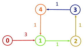
Figure 1: Communication topology A among agents.

VI-A Distributed finite-time differentiator via relative position information

Figure 2: The response curves of relative position estimation under communication topology A.

Figure 3: The response curves of relative velocity estimation under communication topology A.

In the simulation, we set $x_{0}(t)=\sin(t)$, $\delta_{1}(t)=-0.25\sin(0.5t),$ $\delta_{2}(t)=-0.25\cos(0.5t),$ $\delta_{3}(t)=-1.21\cos(1.1t),$ $\delta_{4}(t)=-0.64\sin(0.8t)$, $u_{i}=0,\forall i\in\{1,2,3,4\}$. The initial values of four followers are set as $x_{1}(0)=0,x_{2}(0)=1,x_{3}(0)=1,x_{4}(0)=0.$ The initial values of distributed finite-time differentiator (5) are set as: $\hat{p}_{i}(0)=\hat{q}_{i}(0)=0,\forall i\in\{1,2,3,4\}$. The gains of differentiator are selected as: $k_{1}=5,k_{2}=4$. The response curves of relative position estimation and relative velocity estimation under communication topology A are shown in Fig. 2 and Fig. 3, respectively. It can be seen from the figures that each follower agent can estimate the relative position and relative velocity between itself and the leader in a finite time, which verifies the effectiveness of DFD-R.

VI-B Distributed finite-time differentiator via absolute position information

Figure 4: The response curves of absolute position estimation and absolute velocity estimation under communication topology A.

The signal to be observed is: $f=0.6\sin(t)+0.25\cos(2t)$, thus $\dot{f}=0.6\cos(t)-0.5\sin(2t)$ and $|\ddot{f}|\leq 1.6<l=3$ under a conservative estimate. The initial values of distributed finite-time differentiator (27) are set as: $\hat{p}_{i}(0)=\hat{q}_{i}(0)=0,\forall i\in\{1,2,3,4\}$. The gains of differentiator are selected as: $k_{1}=5,k_{2}=4$. The response curves of absolute position estimation and absolute velocity estimation under communication topology A are shown in Fig. 4. It can be seen from Fig. 4 that each follower agent can estimate the absolute position and absolute velocity of leader in a finite time, which verifies the effectiveness of DFD-A.

VI-C Distributed finite-time consensus controller

Figure 5: The response curves of MAS’ output and control input under communication topology A.

On the basis of works [27, 38], we consider the following leader-follower MAS: $\dot{s}_{0}(t)=a_{0}(t),\dot{s}_{i}(t)=a_{i}(t)+u_{i},$ where $s_{0}$ and $s_{i}$ are the output of leader agent and i-th follower agent respectively, $a_{0}$ and $a_{i}$ are unknown functions with bounded change rate, $u_{i}$ is the control input of i-th follower agent. In this simulation, we set $a_{0}(t)=\cos(t)+0.2\cos(0.2t),a_{1}(t)=\sin(1.5t),a_{2}(t)=2\cos(t),a_{3}(t)=\cos(1.5t),a_{4}(t)=\sin(0.5t)$. Then, $|\dot{a}_{i}(t)-\dot{a}_{0}(t)|\leq 3.1$. For controller (3), $b_{i}=1$ and we set $k_{1}=8,k_{2}=6$, $[v_{1}(0),v_{2}(0),v_{3}(0),v_{4}(0)]=[0,0,0,0]$. The initial values of the system are set as $[s_{0}(0),s_{1}(0),s_{2}(0),s_{3}(0),s_{4}(0)]=[-1,1,1.5,-1,2]$. The response curves of MAS’ output and control input under communication topology A are shown in Fig. 5. Note that the controller is continuous which is chattering-free and is also an advantage by comparing with the discontinuous controller.

VII Conclusion

In this paper, distributed finite-time differentiator (DFD) has been proposed by using relative or absolute position information, and its finite-time stability has been proved by skillfully constructing Lyapunov function. The output consensus of a class of leader-follower MAS has been achieved by extending DFD. In the future, we will try to extend the DFD to higher-order case, and apply the algorithm to formation coordination control by only using relative position information.

References

• [1] A. Levant, โ€Sliding order and sliding accuracy in sliding mode control,โ€ International Journal of Control, 1993, 58: 1247-1263.
• [2] A. Levant, โ€Robust exact differentiation via sliding mode technique,โ€ Automatica, 1998, 34(3): 379-384.
• [3] J. Davila, L. Fridman, A. Levant, โ€Second-order sliding-mode observer for mechanical systems,โ€ IEEE Transactions on Automatic Control, 2005, 50(11): 1785-1789.
• [4] A. Levant, โ€Higher-order sliding modes, differentiation and output feedback control,โ€ International Journal of Control, 2003, 76: 924-961.
• [5] E. Cruz-Zavala, J. A. Moreno and L. M. Fridman, โ€Uniform Robust Exact Differentiator,โ€ IEEE Transactions on Automatic Control, 2011, 56(11): 2727-2733.
• [6] M. T. Angulo, J. A. Moreno, L. Fridman, โ€ Robust exact uniformly convergent arbitrary order differentiator,โ€ Automatica, 2013, 49(8): 2489-2495.
• [7] Y. Pei, H. Gu , K. Liu, J. Lv, โ€An overview on the designs of distributed observers in LTI multi-agent systems,โ€ Science China Technological Sciences, 2021, 64(11) : 2337-2346.
• [8] Y. Hong, J. Hu, L. Gao, โ€Tracking control for multi-agent consensus with an active leader and variable topology,โ€ Automatica, 2006, 42(7): 1177-1182.
• [9] Y. Hong, G. Chen, L. Bushnell, โ€Distributed observers design for leader-following control of multi-agent networks,โ€ Automatica, 2008, 44(3): 846-850.
• [10] S. Park, N. C. Martins, โ€Design of distributed LTI observers for state omniscience,โ€ IEEE Transactions on Automatic Control, 2017, 62(2): 561-576.
• [11] A. Mitra, S. Sundaram, โ€Distributed observers for LTI systems,โ€ IEEE Transactions on Automatic Control, 2018, 63(11): 3689-3704.
• [12] K. Liu, Y. Chen, Z. Duan, J. Lv, โ€Cooperative output regulation of LTI plant via distributed observers with local measurement,โ€ IEEE Transactions on Cybernetics, 2018, 48(7): 2181-2191.
• [13] H. Hong, G. Wen, X. Yu, W. Yu, โ€Robust distributed average tracking for disturbed second-order multiagent systems,โ€ IEEE Transactions on Systems, Man, and Cybernetics: Systems, 2022, 52(5): 3187-3199.
• [14] X. Wang, H. Su, F. Zhang, G. Chen, โ€A robust distributed interval observer for LTI systems,โ€ IEEE Transactions on Automatic Control, doi: 10.1109/TAC.2022.3151586.
• [15] H. Cai, F. L. Lewis, G. Hu, J. Huang, โ€The adaptive distributed observer approach to the cooperative output regulation of linear multi-agent systems,โ€ Automatica, 2017, 75: 299-305.
• [16] Y. Lv, J. Fu, G. Wen, T. Huang, X. Yu, โ€Distributed adaptive observer-based control for output consensus of heterogeneous MASs with input saturation constraint,โ€ IEEE Transactions on Circuits and Systems I: Regular Papers, 2020, 67(3): 995-1007.
• [17] C. He, J. Huang, โ€Adaptive distributed observer for general linear leader systems over periodic switching digraphs,โ€ Automatica, 2022, 137, 110021.
• [18] H. Silm, R. Ushirobira, D. Efimov, J. Richard, W. Michiels, โ€A note on distributed finite-time observers,โ€ IEEE Transactions on Automatic Control, 2019, 64(2): 759-766.
• [19] H. Du, G. Wen, D. Wu, Y. Cheng, J. Lv, โ€Distributed fixed-time consensus for nonlinear heterogeneous multi-agent systems,โ€ Automatica, 2020, 113, 108797.
• [20] H. Cai, J. Huang, โ€Output based adaptive distributed output observer for leader-follower multiagent systems,โ€ Automatica, 2021, 125, 109413.
• [21] T. Liu, Z. Jiang, โ€Distributed formation control of nonholonomic mobile robots without global position measurements,โ€ Automatica, 2013, 49(2): 592-600.
• [22] J. Li, W. Ren, S. Xu, โ€Distributed containment control with multiple dynamic leaders for double-integrator dynamics using only position measurements,โ€ IEEE Transactions on Automatic Control, 2012, 57(6): 1553-1559.
• [23] Q. Ma, S. Xu, โ€Intentional delay can benefit consensus of second-order multi-agent systems,โ€ Automatica, 2023, 147, 110750.
• [24] J. Mei, W. Ren, J. Chen, G. Ma, โ€Distributed adaptive coordination for multiple Lagrangian systems under a directed graph without using neighborsโ€™ velocity information,โ€ Automatica, 2013, 49: 1723-1731.
• [25] J. Mei, W. Ren, G. Ma, โ€Distributed coordination for second-order multi-agent systems with nonlinear dynamics using only relative position measurements,โ€ Automatica, 2013, 49: 1419-1427.
• [26] Y. Lv, G. Wen, T. Huang, Z. Duan, โ€Adaptive attack-free protocol for consensus tracking with pure relative output information,โ€ Automatica, 2020, 117, 108998.
• [27] Y. Cao, W. Ren, โ€Distributed coordinated tracking with reduced interaction via a variable structure approach,โ€ IEEE Transactions on Automatic Control, 2012, 57(1): 33-48.
• [28] Z. Li, X. Liu, W. Ren, L. Xie, โ€Distributed tracking control for linear multiagent systems with a leader of bounded unknown input,โ€ IEEE Transactions on Automatic Control, 2013, 58(2): 518-523.
• [29] S.ย P. Bhat, D.ย S. Bernstein, โ€Finite-time stability of continuous autonomous systems,โ€ SIAM Journal on Control and Optimization, 2000, 38(3), 751-766.
• [30] C. Qian, W. Lin, โ€A continuous feedback approach to global strong stabilization of nonlinear systems,โ€ IEEE Transactions on Automatic Control, 2001, 46(7): 1061-1079.
• [31] G. Hardy, J. Littlewood, G. Polya, Inequalities, Cambridge University Press, Cambridge, 1952.
• [32] L. Wang, F. Xiao, โ€Finite-time consensus problems for networks of dynamic agents,โ€ IEEE Transactions on Automatic Control, 2010, 55(4): 950-955.
• [33] I. Salgado, I. Chairez, J. Moreno, L. Fridman, A. Poznyak, โ€Generalized super-twisting observer for nonlinear systems,โ€ IFAC Proceedings Volumes, 2011, 44(1): 14353-14358.
• [34] J. Fu, G. Wen, W. Yu, T. Huang, X. Yu, โ€Consensus of second-order multiagent systems with both velocity and input constraints,โ€ IEEE Transactions on Industrial Electronics, 2018, 66(10): 7946-7955.
• [35] J. Pliego-Jimenez, M. A. Arteaga-Perez, M. Lopez-Rodriguez, โ€Finite-time control for rigid robots with bounded input torques,โ€ Control Engineering Practice, 2020, 102, 104556.
• [36] H. Du, G. Wen, X. Yu, S. Li, M. Z. Q. Chen, โ€Finite-time consensus of multiple nonholonomic chained-form systems based on recursive distributed observer,โ€ Automatica, 2015, 62: 236-242.
• [37] Y. Cao, W. Ren, Z. Meng, โ€Decentralized finite-time sliding mode estimators and their applications in decentralized finite-time formation tracking,โ€ Systems & Control Letters, 2010, 59: 522-529.
• [38] Y. Cao, W. Ren, โ€Finite-time consensus for multi-agent networks with unknown inherent nonlinear dynamics,โ€ Automatica, 2014, 50: 2648-2656.