Discrete spectra in phase mixing

Abstract

We study solutions of the collisionless Boltzmann equation (CBE) in a functional Koopman representation. This facilitates the use of linear spectral techniques characteristic of the analysis of Schrödinger-type equations. For illustrative purposes, we consider the classical phase mixing of a non-interacting distribution function in a quartic potential. Solutions are determined perturbatively relative to a harmonic oscillator. We impose a form of coarse-graining by choosing a finite dimensional basis to represent the distribution function and time evolution operators, which sets a minimum length scale on phase space structure. We observe a relationship between the dimension of the representation and the multiplicity of the harmonic oscillator eigenvalues. The quartic potential splits the degenerate eigenvalues, which drives mixing in the CBE solution.

1 Introduction

In this paper we investigate the relaxation of collisionless systems through phase mixing. In a statistical description, the macrostate of a system is specified by the phase space distribution function, $f$. This quantifies the probability that a particle exists within an infinitesimal volume of phase space (Sethna, 2006). Liouville’s theorem requires that $f$ is conserved along orbits, and it therefore satisfies the collisionless Boltzmann equation (CBE) (Arnold, 1989). For $s$ spatial degrees of freedom, this is equivalent to the incompressible flow of a $2s$ dimensional fluid in a velocity field specified by Hamilton’s equations. An introductory description of this can be found in Binney & Tremaine (2008), but we summarize as follows. Let us assume an anharmonic potential in which orbital frequency of test particles is dependent on their amplitudes of oscillation. In the fluid analogy, this means that vorticity of the velocity field depends on the spatial coordinate. A distribution out of equilibrium with such a potential will deform with time as packets of density with different energies orbit at varying frequencies. For a fixed conservative Hamiltonian this continues indefinitely, with different energy orbits becoming increasingly out of phase with each other. In this process, the scale of structure in the distribution decreases. Eventually when the scale becomes so small that adjacent wraps of the mixed distribution become indistinguishable, the system has equilibrated.

Phase mixing in general leads to complex structures, especially for the $s=3$ case present in galactic dynamics and cosmology (Tremaine, 1999; Perrett et al., 2003; Abel et al., 2012). Even for $s=1$, which applies to considerations of the vertical motion in the Galactic disc, this process is not trivial. With astrometric data from Gaia Collaboration et al. (2018), a one armed spiral was observed in the vertical phase space of solar neighborhood stars (Antoja et al., 2018). In reality this is a $s=3$ system, as it is unlikely that the vertical dynamics are decoupled from motion in the plane (Hunt et al., 2021), but much attention has been given to the structure in the univariate case (Schönrich & Binney, 2018; Darling & Widrow, 2019a; Bennett & Bovy, 2018, 2021). At present, no models have reproduced the exact form of the Gaia spiral.

In Darling & Widrow (2019b), it was suggested that the phase mixing process can be represented with the discrete spectrum of a linear time-evolution operator of finite dimension. There, eigenfunctions were estimated numerically from the full temporal history of a system by applying Dynamic Mode Decomposition (DMD) (Mezić, 2005; Rowley et al., 2009; Kutz et al., 2016) to $N$-body simulations. This served to investigate the claim that self-gravity should not be ignored in phase mixing (Darling & Widrow, 2019a), as well as to explore the representation of this process with persistent oscillatory structures. Stable oscillations such as bending and breathing modes were observed in a self-interacting system in an anharmonic potential. When modifying the relative dominance of self-interaction and anharmonic forcing, these oscillatory structures were more prominent the closer the system was to purely self-interacting. For stronger anharmonic forcing, they were deformed to include spiral structure.

DMD is closely related to Koopman theory (Koopman, 1931), which supposes that a complex, potentially nonlinear system can be represented as a simpler linear one by studying its evolution in terms of observable functions of its state space. This concept was used to interpret the results in Darling & Widrow (2019b), arguing that the binning of $N$-body simulations constituted a mapping to observables. Because of the numerical nature of that work, it was difficult to study the supposed mechanism of phase mixing from discrete modes, or establish a concrete connection to Koopman theory. The DMD approach also draws comparison to the use of multichannel singular spectrum analysis (mSSA) (Weinberg & Petersen, 2021; Johnson et al., 2023). In both cases, principle component analysis (PCA) based techniques are applied to time-series data, but in the mSSA papers time series comprise basis function expansion coefficients rather than histogrammed $N$-body results.

In the present work, we aim to investigate a mechanism of phase mixing with a discrete linear operator spectrum, emphasizing the role of representation scale, and properties of the spectrum. The essential premise is that the minimum length scale and algebraic multiplicity of evolution operator eigenvalues depend on the dimension of the representation. Splitting of degenerate eigenvalues by anharmonic forcing causes differential rotation in the distribution function, manifesting as phase mixing. The system dynamics are determined in terms of basis function expansion coefficients, which we treat as functionals of $f$, adopting a functional Koopman formalism for our calculations. In doing so, we apply techniques from degenerate perturbation theory of the Schrödinger equation. All of our calculations are carried out symbolically.

This paper is organized as follows. In Section 2 we define our coordinates and Hamiltonian, as well as the vector spaces in which we perform our calculations. In section 3 we define the time evolution operator for functionals of $f$, and then restate the problem in this formalism. In Section 4 we define a matrix representation for our operators, and compute the harmonic oscillator spectrum. Section 5 contains the perturbative treatment of the anharmonic potential, and a description of the eigenvalue splitting mechanism for phase mixing. Sections 6 and 7 contain a discussion of connections to other works, and concluding remarks on foreseeable extensions.

2 Preliminaries

Consider a two-dimensional phase space comprising position $\bar{q}$ and momentum $\bar{p}$. We concern ourselves with the phase space distribution function, $f(\bar{q},\bar{p})$. This is defined such that,

$$\mathrm{P}\bigl{(}\bar{q},\bar{p}\in\mathcal{R}\bigr{)}=\int_{\mathcal{R}}d\bar{q}d\bar{p}\ f(\bar{q},\bar{p}),$$ (1)

is the probability of finding a particle in the region of phase space, $\mathcal{R}$. The dynamics of $f$ are prescribed by the Hamiltonian density, $h(\bar{q},\bar{p})$, according to the CBE,

$$\frac{\partial f}{\partial t}+[f,h]=0.$$ (2)

Here $[f,h]=\frac{\partial f}{\partial q}\frac{\partial h}{\partial p}-\frac{\partial f}{\partial p}\frac{\partial h}{\partial q}$ denotes the Poisson bracket.

2.1 System Hamiltonian

We begin with the Hamiltonian density for a harmonic oscillator with frequency $\kappa$,

$$h_{0}(\bar{q},\bar{p})=\tfrac{1}{2}\left(\bar{p}^{2}+\kappa^{2}\bar{q}^{2}\right).$$ (3)

This is to be understood as the standard kinematic term plus the leading term in a Taylor series of any even potential. By Jeans’ theorem, the Hamiltonian defines the coordinate dependence of the equilibrium distribution function. Let us choose

$$f_{0}(\bar{q},\bar{p})=\frac{1}{Z}\mathrm{e}^{-\frac{1}{2}\beta h_{0}(\bar{q},\bar{p})}.$$ (4)

Here, $\beta$ is a coldness parameter inversely proportional to the velocity dispersion, and $Z$ is the partition function. It is convenient to work with scaled dimensionless coordinates, so we let

$$\bar{q}=\tfrac{1}{\kappa}\sqrt{\tfrac{2}{\beta}}q,\ \ \bar{p}=\sqrt{\tfrac{2}{\beta}}p.$$ (5)

In these coordinates, the Hamiltonian density and distribution function become

$$h_{0}(q,p)=\frac{1}{\beta}\left(q^{2}+p^{2}\right),\ \ f_{0}(q,p)=\frac{1}{Z}\mathrm{e}^{-\frac{1}{2}(q^{2}+p^{2})}.$$ (6)

Now we add an anharmonic correction of the form $\varphi\bar{q}^{4}$, representative of the next term in the even Taylor series. Our total Hamiltonian density in scaled coordinates is

$$h(q,p)=h_{0}(q,p)+\varphi\frac{4}{\kappa^{4}\beta^{2}}q^{4}.$$ (7)

The factor $4\kappa^{-4}\beta^{-2}$ comes from the coordinate transformation in equation 5. We will use $\varphi=-\frac{\beta}{12}(\frac{\kappa}{2})^{4}$ in our calculations. This is chosen to assure stable orbits for a range of initial conditions while introducing vorticity that decreases with position, of which the effects can be seen within a few dynamical times.

2.2 Space of bivariate functions

Any configuration of $f$ is an element of a function space defined for the independent variables $q$ and $p$. Denote by $\mathscr{H}$ the space of functions of $q$ and $p$ on a domain $\mathcal{D}$. This space is equipped with an inner product, which for any pair $g_{1},g_{2}\in\mathscr{H}$ is

$$\langle g_{1},g_{2}\rangle=\int_{\mathcal{D}}dqdp\ g_{1}(q,p)g_{2}^{\dagger}(q,p),$$ (8)

where ^† indicates complex conjugation. The inner product possesses conjugate symmetry, $\langle g_{1},g_{2}\rangle^{\dagger}=\langle g_{2},g_{1}\rangle$.

Suppose that there exists a set of linearly independent functions $\{e_{j,k}\}$ that form a basis in $\mathscr{H}$. We use two indices here for the two variables $q$ and $p$. Any function $g\in\mathscr{H}$ can be written in terms of the basis functions as

$$g(q,p)=\sum_{j=0}^{\infty}\sum_{k=0}^{\infty}\langle e_{j,k},g\rangle e_{j,k}(q,p).$$ (9)

2.3 Conjugate space of functionals

Given the function space $\mathscr{H}$, one may consider another, distinct vector space housing its functionals. Such a space is called dual to $\mathscr{H}$, and is denoted $\mathscr{H}^{*}$. For the purposes of this work, we refer to a functional of $f$ as any linear mapping

$$G[f]=\langle f,g\rangle,$$ (10)

which takes the input function, here the distribution function $f$, and maps it to $\mathbb{C}$ by integration with a given $g$. For every $g\in\mathscr{H}$, there is a unique $G\in\mathscr{H}^{*}$ given by equation 10 (Riesz representation theorem, see for example Conway (1994)). In the present context, the input function will always be $f$, and it is treated as a variable relative to a functional $G[f]\in\mathscr{H}^{*}$ in the same sense that $q$ and $p$ are variables with respect to a function $g(q,p)\in\mathscr{H}$.

The dual space $\mathscr{H}^{*}$ has an inner product and basis that can be understood in terms of the corresponding constructions in $\mathscr{H}$. Given a basis $\{e_{j,k}\}$ of $\mathscr{H}$, there exists a basis for $\mathscr{H}^{*}$, $\{E_{j,k}\}$. The two are related by the biorthonormal condition, $E_{j,k}[e_{j^{\prime},k^{\prime}}]=\delta_{j}^{j^{\prime}}\delta_{k}^{k^{\prime}}$. The inner product of any two $G_{1},G_{2}\in\mathscr{H}^{*}$ is

$$\langle G_{1},G_{2}\rangle_{*}=\bigg{\langle}\frac{\delta G_{2}}{\delta f},\frac{\delta G_{1}}{\delta f}\bigg{\rangle},$$ (11)

where the $\langle\ ,\ \rangle_{*}$ (with asterisk) specifies that the operation is in $\mathscr{H}^{*}$, and $\frac{\delta}{\delta f}$ denotes the functional derivative with respect to $f$. For any linear functional $G=\langle f,g\rangle$, this is such that $\frac{\delta G}{\delta f}=g$.

Finally we highlight some important quantities that exist in $\mathscr{H}^{*}$. The total energy, which is the expectation value of the Hamiltonian with respect to $f$, is the functional $H[f]=\langle f,h\rangle$. Additionally, if we project $f$ onto a set of basis functions in $\mathscr{H}$ as in equation 9, the coefficients are the functionals $E_{j,k}^{\dagger}$. If we study the dynamics of $E_{j,k}$ according to $H$ in $\mathscr{H}^{*}$, we obtain the time-evolution of the basis function expansion coefficients.

2.4 Particular choice of basis functions

We choose as a basis for $\mathscr{H}$ products of univariate Gaussian-Hermite functions. That is,

$$e_{j,k}(q,p)=N_{j,k}f_{0}(q,p)P_{j}(q)P_{k}(p),$$ (12)

where $P_{j}(x)$ denotes the $j$th Hermite polynomial of either $q$ or $p$, and $N_{j,k}$ is a normalization constant,

$$N_{j,k}=\frac{Z}{\sqrt{\pi 2^{j+k}j!k!}}.$$ (13)

The corresponding functionals are $E_{j,k}[f]=\langle f,e_{j,k}\rangle$. Our chosen bivariate functions inherit orthogonality from the Hermite polynomials. Explicitly,

$$\langle e_{j,k},e_{j^{\prime},k^{\prime}}\rangle=\delta_{j^{\prime}}^{j}\delta_{k^{\prime}}^{k}.$$ (14)

This applies to the entire real number line in both variables, so our domain $\mathcal{D}$ is set to the entire phase space. Note that the Hermite polynomials satisfy the following two recurrence relations:

$$\frac{d}{dx}P_{j}(x)=2jP_{j-1}(x),$$ (15)

$$xP_{j}(x)=\frac{1}{2}P_{j+1}(x)+jP_{j-1}(x).$$ (16)

3 Dynamics

In what follows, we will use the notion of a flow map. This is an operator on $\mathscr{H}$ denoted $\hat{S}^{t}$, which takes an initial state $f$ to another state at time $t$, $\hat{S}^{t}f$. The particular action of $\hat{S}^{t}$ is prescribed by the CBE (equation 2).

3.1 Time evolution operator for functionals

Knowing the flow map $\hat{S}^{t}$ is tantamount to solving equation 2. Here, we leverage Koopman (1931) to effectively apply the flow map, without dealing explicitly with the CBE. Discussion of the Koopman formalism in the context of astrophysics can be found in Darling & Widrow (2019b) and Darling & Widrow (2021), but for a more rigorous description of the functional realization we will use here, see Nakao & Mezić (2020). Briefly, the idea is that rather than consider the distribution function directly, one can instead look at the dynamics of “observables”. In the case of a partial differential equation like the CBE, the observables take the form of functionals, $G[f]$. Let us define a time evolution operator that acts on $\mathscr{H}^{*}$, which we denote $\hat{U}^{t}$. This linear operator is defined as the composition of any $G\in\mathscr{H}^{*}$ and the flow map $\hat{S}^{t}$. That is,

$$\hat{U}^{t}G[f]=G[\hat{S}^{t}f].$$ (17)

If it is easier to determine the action of $\hat{U}^{t}$ than $\hat{S}^{t}$, one can compute the functional $\hat{U}^{t}G$ which encodes information about $f$ at time $t$. Subsequently, if we know how to infer $f$ from a functional or set of functionals, we can compute the future state $\hat{S}^{t}f$.

Treating $\hat{U}^{t}G$ as a function of $t$, we may write its infinitesimal change with respect to $t$ as

$$\frac{d}{dt}\hat{U}^{t}G[f]=\lim_{\tau\rightarrow 0}\frac{\hat{U}^{t+\tau}G[f]-\hat{U}^{t}G[f]}{\tau}.$$ (18)

To evaluate the $\tau$ limit, we separate out the $\hat{U}^{t}$ (by linearity), and apply equation 17 for $\hat{U}^{\tau}G$. That is,

$$\frac{d}{dt}\hat{U}^{t}G[f]=\hat{U}^{t}\left(\lim_{\tau\rightarrow 0}\frac{G[\hat{S}^{\tau}f]-G[f]}{\tau}\right).$$ (19)

For small $\tau$, $\hat{S}^{\tau}f=f+\tau[h,f]+\mathcal{O}(\tau^{2})$. Replacing $G[\hat{S}^{\tau}f]$ in equation 19 with this takes care of the limit, and we are left with

$$\frac{d}{dt}\hat{U}^{t}G[f]=\Bigl{\langle}[h,f],\frac{\delta}{\delta f}\hat{U}^{t}G\Bigr{\rangle}\coloneqq\hat{A}\Bigl{(}\hat{U}^{t}G[f]\Bigr{)}.$$ (20)

Here we have defined as $\hat{A}$ the infinitesimal generator of $\hat{U}^{t}$. This is another operator on $\mathscr{H}^{*}$, and will be the focus of much of this work. To be clear, the action of $\hat{A}$ on any $G\in\mathscr{H}^{*}$ is

$$\hat{A}G=\Bigl{\langle}[h,f],\frac{\delta G}{\delta f}\Bigr{\rangle}=\Bigl{\langle}f,\left[\frac{\delta G}{\delta f},\frac{\delta H}{\delta f}\right]\Bigr{\rangle}.$$ (21)

The final equality is obtained by expanding the Poisson bracket and performing integration by parts with respect to $p$ on the first term and $q$ on the second. This final form is called a Morrison bracket, which originates in plasma physics (Morrison, 1980). We denote this multiplicative operation between vectors in $\mathscr{H}^{*}$ by $[G,H]_{f}$, indicating that it is the bracket between $G$ and $H$ with respect to $f$. We prefer this form, as it makes clear that a functional $G$ acted on by $\hat{A}$ is another vector in $\mathscr{H}^{*}$. If we let $g=\frac{\delta G}{\delta f}$, $\hat{A}G$ maps the expectation value of $g$ to that of $[g,h]$. An operator of this form has appeared in the gravitational context previously in for example Perez (2005), where the Morrison bracket is used to form a so-called functional Vlasov equation.

Equation 20 is a Schrödinger-type equation. It follows that the operator $\hat{U}^{t}$ satisfies an ordinary differential equation, and has the general solution

$$\hat{U}^{t}=\mathrm{e}^{\int_{0}^{t}d\tau\hat{A}}.$$ (22)

The reader familiar with quantum mechanics (QM) may find that this resembles the Heisenberg representation, with $\hat{A}$ analogous to the Hamiltonian operator. Like in QM, we can construct solutions to equation 20 by solving the associated eigenvalue problem of $\hat{A}$.

3.2 Time evolution of $f$

Denote the $j$th eigenvalue and eigenfunctional of $\hat{A}$ by $\lambda_{j}$ and $\Psi_{j}[f]$ respectively. The eigenvalue problem is then, $\hat{A}\Psi_{j}=\lambda_{j}\Psi_{j}$. Let $\psi_{j}(q,p)=\frac{\delta\Psi_{j}}{\delta f}$. For convenience, we call this quantity an eigenfunction of $\hat{A}$, but really it is an eigenfunction of the Liouville operator, $[h,\cdot]$. Suppose that $\{\psi_{j}\}$ forms a basis of $\mathscr{H}$, and $\{\Psi_{j}\}$ of $\mathscr{H}^{*}$. For $\frac{\partial\hat{A}}{\partial t}=0$, equation 22 simplifies to $\hat{U}^{t}=\mathrm{e}^{\hat{A}t}$, and we have

$$\hat{U}^{t}\Psi_{j}[f]=\Psi_{j}[\hat{S}^{t}f]=\mathrm{e}^{\lambda_{j}t}\Psi_{j}[f].$$ (23)

By conjugate symmetry of the inner product, the expansion coefficient of $f$ onto $\psi_{j}$ at time $t$ is then

$$\langle\psi_{j},\hat{S}^{t}f\rangle=\Psi^{\dagger}_{j}[\hat{S}^{t}f]=\mathrm{e}^{\lambda_{j}^{\dagger}t}\langle\psi_{j},f\rangle.$$ (24)

Applying $\hat{S}^{t}$ to equation 9 and using this result, $\hat{S}^{t}f$ is

$$\hat{S}^{t}f(q,p)=\sum_{j=1}^{\infty}\langle\psi_{j},f\rangle\mathrm{e}^{\lambda_{j}^{\dagger}t}\psi_{j}(q,p).$$ (25)

3.3 Restatement of the problem

Now that we have established the formalism in which we will carry out our calculations, it is advantageous to restate the original problem. Recall that the target Hamiltonian is stated in equation 7. In terms of total energy functionals, this corresponds to $H=H_{0}+\varphi H_{4}$, where $H_{0}=\langle f,h_{0}\rangle$ and $H_{4}=\langle f,\frac{4}{\kappa^{4}\beta^{2}}q^{4}\rangle$. It follows that the generators are $\hat{A}_{0}=[\cdot,H_{0}]_{f}$ and $\hat{A}_{4}=[\cdot,H_{4}]_{f}$. The total generator is $\hat{A}=\hat{A}_{0}+\varphi\hat{A}_{4}$. Our goal then is to compute the spectrum of $\hat{A}$, so that we can use equation 25.

4 Matrix Representation

To carry out calculations, we map the quantities in $\mathscr{H}^{*}$ to finite dimensional matrices and vectors. We begin by choosing a finite dimension, $M\in\mathbb{N}$. If we take all bivariate Hermite polynomials up to order $N$, the dimension of our finite basis is $M=\frac{1}{2}(N+1)(N+2)$. We define a reference vector for the $\mathscr{H}$ basis as

$$\mathbf{u}=\left(e_{0,0},\cdots,e_{N,0},\cdots,e_{0,N}\right).$$ (26)

This is a vector-valued function of the phase space coordinates. For any vector $\mathbf{v}\in\mathbb{C}^{M}$, the contraction $\mathbf{u}^{\dagger}\cdot\mathbf{v}$ returns a linear combination of the basis functions. Note that for vectors and matrices, ^† (introduced as complex conjugation in Section 2.2) is the conjugate transpose.

When we choose the dimension $M$ for the matrix representation, we introduce coarse-graining by imposing a minimum length scale. The resultant scale is set by the maximum polynomial order $N$, and the model parameters that appear in the coordinate scaling (equation 5). The minimum scale can be quantified by the distance between adjacent roots in the highest order polynomial appearing in the basis functions, $e_{j,k}$.

4.1 Matrix Elements of $\hat{A}_{0}$

In order to compute the spectrum of $\hat{A}_{0}$, we construct a $M\times M$ matrix, which we denote $\bm{\mathsf{A}}_{\mathsf{0}}$. Its elements are obtained by computing the inner products,

$$\left(\bm{\mathsf{A}}_{\mathsf{0}}\right)_{j^{\prime},k^{\prime}}^{j,k}=\langle E_{j^{\prime},k^{\prime}},\hat{A}_{0}E_{j,k}\rangle_{*}.$$ (27)

Substituting $G\rightarrow E_{j,k}$, and $H\rightarrow H_{0}$ into equation 21, and applying the definition of the $\mathscr{H}^{*}$ inner product in equation 11, we obtain

$$\left(\bm{\mathsf{A}}_{\mathsf{0}}\right)_{j^{\prime},k^{\prime}}^{j,k}= \langle e_{j^{\prime},k^{\prime}}(q,p),[h_{0}(q,p),e_{j,k}(q,p)]\rangle.$$ (28)

Expanding the Poisson bracket, and applying equation 15 we are left with the set of integrals,

$$\left(\bm{\mathsf{A}}_{\mathsf{0}}\right)_{j^{\prime},k^{\prime}}^{j,k}= \kappa N_{j^{\prime},k^{\prime}}N_{j,k}\int_{\mathcal{D}}dqdpf_{0}^{2}(q,p)$$ (29)

$$\times\bigg{(}kqP_{j^{\prime}}(q)P_{j}(q)P_{k^{\prime}}(p)P_{k-1}(p)$$

$$-jpP_{k^{\prime}}(p)P_{k}(p)P_{j^{\prime}}(q)P_{j-1}(q)\bigg{)}.$$

The integrals are easier to evaluate if we first apply equation 16. Doing so for $qP_{j}(q)$ in the first term and $pP_{k}(p)$ in the second gives

$$\left(\bm{\mathsf{A}}_{\mathsf{0}}\right)_{j^{\prime},k^{\prime}}^{j,k}= \frac{\kappa}{2}N_{j^{\prime},k^{\prime}}N_{j,k}\int_{\mathcal{D}}dqdpf_{0}^{2}(q,p)$$ (30)

$$\times\bigg{(}kP_{j^{\prime}}(q)P_{j+1}(q)P_{k^{\prime}}(p)P_{k-1}(p)$$

$$-jP_{k^{\prime}}(p)P_{k+1}(p)P_{j^{\prime}}(q)P_{j-1}(q)\bigg{)}.$$

From the orthogonality of the Hermite polynomials with respect to $f_{0}^{2}$, this reduces to

$$\left(\bm{\mathsf{A}}_{\mathsf{0}}\right)_{j^{\prime},k^{\prime}}^{j,k}=\kappa\bigg{(}\sqrt{k(j+1)}\delta_{j^{\prime}}^{j+1}\delta_{k^{\prime}}^{k-1}-\sqrt{j(k+1)}\delta_{k^{\prime}}^{k+1}\delta_{j^{\prime}}^{j-1}\bigg{)}.$$ (31)

We organize the resulting $M^{2}$ real numbers into an $M\times M$ matrix according to the ordering of the $e_{j,k}$ indices in the reference vector $\mathbf{u}$ (equation 26).

4.2 Spectrum of $\hat{A}_{0}$

With a matrix representation of $\hat{A}_{0}$, we can compute a subset of its spectrum. Let $\bm{\mathsf{A}}_{\mathsf{0}}\bm{\Psi}^{(0)}=\bm{\Psi}^{(0)}\bm{\Lambda}^{(0)}$ denote the eigendecomposition of $\bm{\mathsf{A}}_{\mathsf{0}}$, where

$$\bm{\Psi}^{(0)}=\begin{pmatrix}|&|&&\\ \bm{\psi}_{1}^{(0)}&\bm{\psi}_{2}^{(0)}&\cdots&\\ |&|&&\ \end{pmatrix},\ \ \bm{\Lambda}^{(0)}=\begin{pmatrix}\lambda_{1}^{(0)}&0&\cdots\\ 0&\lambda_{2}^{(0)}&\\ \vdots&&\ddots\\ \end{pmatrix}.$$ (32)

Here, $\bm{\psi}_{j}^{(0)}\in\mathbb{C}^{M}$ and $\lambda_{j}^{(0)}\in\mathbb{C}$. We can transform the eigenvectors of $\bm{\mathsf{A}}_{\mathsf{0}}$ into eigenfunctions of $\hat{A}_{0}$ by taking their contraction with the reference vector $\mathbf{u}$. Denoting the eigenfunctions of $\hat{A}_{0}$ by $\psi_{j}^{(0)}(q,p)$, we have

$$\psi_{j}^{(0)}(q,p)=\mathbf{u}^{\dagger}\cdot\bm{\psi}_{j}^{(0)}.$$ (33)

In general, there can be a combination of real and imaginary eigenvalues, with varying algebraic multiplicity, $d_{j}$. The complex eigenvalues come in conjugate pairs, as do their associated eigenvectors. We will assume that all of the eigenvectors are linearly independent, including those associated with the repeated eigenvalues. This means that although we have eigenvalues with algebraic multiplicity $d_{j}>1$, they all have geometric multiplicity of 1. Though the algebraic multiplicities of the $\hat{A}_{0}$ eigenvalues do not pose an issue for the harmonic oscillator, we will need to handle them more carefully when computing corrections for the anharmonic potential.

We show in Fig. 1 bending and breathing modes associated with $\lambda_{j}^{(0)}=-i\kappa$ and $\lambda_{j}^{(0)}=-i2\kappa$ respectively. In each case, the presented structure is the real part of one member of a conjugate pair. When the full complex functions are taken together with their conjugates, multiplication with the relevant complex exponentials produces real valued clockwise rotating bending and breathing patterns.

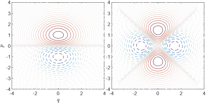
Figure 1: Level set contours of two $\hat{A}_{0}$ eigenfunctions, denoted $\psi_{j}^{(0)}(q,p)$. On the left is a bending mode for $\lambda_{j}^{(0)}=-\mathrm{i}\kappa$ and on the right is a breathing mode for $\lambda_{j}^{(0)}=-\mathrm{i}2\kappa$. Each are one of four linearly independent functions associated with their respective eigenvalue. We show only the real part of each, noting that the imaginary parts in this case differ only by a rotation.

4.3 Dynamics of $f$ from $\hat{A}_{0}$

The dynamics of an arbitrary initial condition according to $h_{0}$ are determined by the spectrum of $\hat{A}_{0}$. Explicitly, $f$ is mapped to a new function $\hat{S}_{0}^{t}f$ at time $t$ by the flow of equation 2, for $h=h_{0}$. We have from equation 25,

$$\hat{S}_{0}^{t}f(q,p)=\sum_{j=1}^{M}\langle\psi_{j}^{(0)},f\rangle\mathrm{e}^{\lambda_{j}^{\dagger(0)}t}\psi_{j}^{(0)}(q,p).$$ (34)

For the harmonic potential, the dynamics of $f$ are a rigid rotation of the initial condition about the origin. It is not immediately apparent from equation 34, but we can verify that no deformation to the distribution occurs with the conserved quantities in the spectrum of $\hat{A}_{0}$. There are several eigenvectors of $\bm{\mathsf{A}}_{\mathsf{0}}$ associated with a zero eigenvalue. Each of these corresponds to a conserved quantity. We have the sequence:

$$\psi_{1}^{(0)}(q,p) =e_{0,0},$$ (35)

$$\psi_{2}^{(0)}(q,p) =\tfrac{\sqrt{2}}{2}\left(e_{2,0}+e_{0,2}\right),$$

$$\psi_{3}^{(0)}(q,p) =\tfrac{1}{4}\left(\sqrt{6}e_{4,0}+2e_{2,2}+\sqrt{6}e_{0,4}\right),$$

$$\psi_{4}^{(0)}(q,p) =\tfrac{1}{4}\left(\sqrt{5}e_{6,0}+\sqrt{3}e_{4,2}+\sqrt{3}e_{2,4}+\sqrt{5}e_{0,6}\right)...$$

The first two correspond to conservation of phase space density and energy, and are themselves constants of motion in the sense that $[\psi_{1}^{(0)},h_{0}]=[\psi_{2}^{(0)},h_{0}]=0$. The other eigenfunctions are not conserved in this sense. It is rather the corresponding functionals which are conserved. This can be understood in terms of the weighted statistical moments of $f$, defined as $F_{m,n}[f]=\langle f,f_{0}\ q^{m}p^{n}\rangle$. All of the zero-eigenvalue functions in equation 35 contain even polynomials of $q$ and $p$. This means that the corresponding functionals $\langle f,\psi_{j}^{(0)}\rangle$ are linear combinations of bivariate moments $F_{m,n}$ corresponding only to even powers in both variables. Such moments are variance, covariance, kurtosis, cokurtosis and so on. These moments quantify the character of symmetric properties of the distribution, ignoring asymmetries like mean and skew. This means that when the integrals over phase space are carried out, the result is the same regardless of where along the harmonic oscillator orbit the distribution is. Any deformation in $f$ will change the values of the integrals in this sequence. Their presence as zero-eigenvalue functionals in the spectrum of $\hat{A}_{0}$ restricts the dynamics to rigid rotation.

5 Anharmonic Potential

With the harmonic oscillator spectrum calculated, we can now proceed to estimating the spectrum of $\hat{A}$. We begin by computing the matrix elements of $\hat{A}_{4}$.

5.1 Matrix elements of $\hat{A}_{4}$

The equivalent expression to equation 28 for the $\hat{A}_{4}$ matrix elements is obtained by making the substitutions $G\rightarrow E_{j,k}$, and $H\rightarrow H_{4}$ in equation 21. We have,

$$\left(\bm{\mathsf{A}}_{\mathsf{4}}\right)_{j^{\prime},k^{\prime}}^{j,k}= \Bigl{\langle}e_{j^{\prime},k^{\prime}}(q,p),\left[\tfrac{4}{\kappa^{4}\beta^{2}}q^{4},e_{j,k}(q,p)\right]\Bigr{\rangle}.$$ (36)

We evaluate the Poisson bracket, applying equation 15 to the Hermite polynomial derivatives, and equation 16 to the $f_{0}$ derivatives. We are left with

$$\left(\bm{\mathsf{A}}_{\mathsf{4}}\right)_{j^{\prime},k^{\prime}}^{j,k}= \frac{8}{\kappa^{3}\beta}N_{j^{\prime},k^{\prime}}N_{j,k}\int_{\mathcal{D}}dqdpf_{0}^{2}(q,p)q^{3}P_{j^{\prime}}(q)P_{j}(q)$$ (37)

$$\times P_{k^{\prime}}(p)\left(kP_{k-1}(p)-\tfrac{1}{2}P_{k+1}(p)\right).$$

To evaluate the these integrals for all indices, it is easiest to re-write $q^{3}P_{j}(q)$ strictly in terms of Hermite polynomials. Recursive application of equation 16 yields (for arbitrary $n\in\mathbb{N}$) an expansion of the form

$$x^{n}P_{j}(x)=\sum_{m=0}^{n}b_{m}(j)P_{j+n-2m}(x),$$ (38)

where the coefficients $b_{m}(j)$ are polynomials in $j$ of order $m$. Table 1 contains a list of the relevant coefficients for both a quartic and sextic potential. To compute the contribution from $q^{3}P_{j}(q)$, let us define the integral

$$I_{j^{\prime}}^{j} =\int_{-\infty}^{+\infty}dq\ \mathrm{e}^{-q^{2}}q^{3}P_{j^{\prime}}(q)P_{j}(q).$$ (39)

Application of equation 38, with the coefficients from the $n=3$ column of Table 1 yields

$$I_{j^{\prime}}^{j}=\sum_{m=0}^{3}b_{m}(j)\int_{-\infty}^{+\infty}dq\ \mathrm{e}^{-q^{2}}P_{j^{\prime}}(q)P_{j+3-2m}(q).$$ (40)

This is evaluated easily by the orthogonality of the Hermite polynomials, leaving

$$I_{j^{\prime}}^{j}=\sum_{m=0}^{3}b_{m}(j)\left(\sqrt{\pi}2^{j+3-2m}(j+3-2m)!\right)^{\tfrac{1}{2}}\delta_{j^{\prime}}^{j+3-2m}.$$ (41)

Now we replace the relevant terms in equation 37 with the evaluated $I_{j^{\prime}}^{j}$, and compute the remaining momentum space integral. We are left with

$$\left(\bm{\mathsf{A}}_{\mathsf{4}}\right)_{j^{\prime},k^{\prime}}^{j,k}= \frac{4\varphi}{\kappa^{3}\beta}\sum_{m=0}^{3}b_{m}(j)N_{j,k}\delta_{j^{\prime}}^{j+3-2m}$$ (42)

$$\times\left(\frac{2k\delta_{k^{\prime}}^{k-1}}{N_{j+3-2m,k-1}}-\frac{\delta_{k^{\prime}}^{k+1}}{N_{j+3-2m,k+1}}\right).$$

Again, we organize the resulting values into an $M\times M$ matrix according to the ordering of indices in $\mathbf{u}$.

$m$	$b_{m}$ $(n=3)$	$b_{m}$ $(n=5)$
0	$2^{-3}$	$2^{-5}$
1	$\frac{3}{4}(j+1)$	$\frac{1}{2}(j+\frac{5}{4})$
2	$\frac{3}{2}j^{2}$	$\frac{5}{2}(\frac{1}{2}j^{2}+j+\frac{3}{4})$
3	$j!/(j-3)!$	$\frac{5}{2}j(j^{2}+\frac{1}{2})$
4		$5j(\frac{1}{2}j^{3}-2j^{2}+\frac{5}{2}j-1)$
5		$j!/(j-5)!$

Table 1: Coefficients for Hermite polynomial expansion of matrix element integrand as in equation 38.

5.2 Spectrum of $\hat{A}$

To apply the ordinary differential equation solution for $\hat{U}^{t}$, and compute $\hat{S}^{t}f$ from equation 25, we need the spectrum of $\hat{A}$. The matrix

$$\bm{\mathsf{A}}=\bm{\mathsf{A}}_{\mathsf{0}}+\varphi\bm{\mathsf{A}}_{\mathsf{4}},$$ (43)

does not admit a diagonalization directly, so we adopt a perturbative treatment. We follow a standard procedure for analysis of the Schrödinger equation in QM (for an introductory description, see for example Griffiths & Schroeter (2018)). Suppose that the eigenvalues and eigenvectors of $\bm{\mathsf{A}}$ can be written as a power series in the parameter $\varphi$. That is,

$$\lambda_{j}(\varphi) =\lambda_{j}^{(0)}+\varphi\lambda_{j}^{(1)}+\mathcal{O}(\varphi^{2}),$$ (44)

$$\bm{\psi}_{j}(\varphi) =\bm{\psi}_{j}^{(0)}+\varphi\bm{\psi}_{j}^{(1)}+\mathcal{O}(\varphi^{2}).$$

We assume that these quantities satisfy the eigenvalue problem,

$$\left(\bm{\mathsf{A}}_{\mathsf{0}}+\varphi\bm{\mathsf{A}}_{\mathsf{4}}\right)\bm{\psi}_{j}(\varphi)=\lambda_{j}(\varphi)\bm{\psi}_{j}(\varphi).$$ (45)

Substituting the expressions in equation 44 into 45 and equating terms of equal power in $\varphi$, we obtain a sequence of equations relating the power series coefficients and the operators $\bm{\mathsf{A}}_{\mathsf{0}}$ and $\bm{\mathsf{A}}_{\mathsf{4}}$. The zero order equation is the eigenvalue problem for $\bm{\mathsf{A}}_{\mathsf{0}}$, stated in Section 4.2. The first order equation is

$$\left(\bm{\mathsf{A}}_{\mathsf{0}}-\lambda_{j}^{(0)}\right)\bm{\psi}_{j}^{(1)} =\left(\lambda^{(1)}_{j}-\bm{\mathsf{A}}_{\mathsf{4}}\right)\bm{\psi}_{j}^{(0)}.$$ (46)

We assume that the basis formed by the eigenvectors of $\bm{\mathsf{A}}_{\mathsf{0}}$ spans the eigenspace of $\bm{\mathsf{A}}$. That is,

$$\bm{\psi}_{j}(\varphi)=\sum_{k=1}^{M}\left({\bm{\psi}_{k}^{(0)}}^{\dagger}\cdot\bm{\psi}_{j}(\varphi)\right)\bm{\psi}_{k}^{(0)}.$$ (47)

Note that ${\bm{\psi}_{k}^{(0)}}^{\dagger}\cdot\bm{\psi}_{j}(\varphi)$ indicates a dot product in $\mathbb{C}^{M}$ and the result is scalar. Substituting $\bm{\psi}_{j}(\varphi)$ as in equation 44 into equation 47, we express the first order correction as

$$\bm{\psi}_{j}^{(1)}=\sum_{k=1}^{M}\left({\bm{\psi}_{k}^{(0)}}^{\dagger}\cdot\bm{\psi}_{j}^{(1)}\right)\bm{\psi}_{k}^{(0)}.$$ (48)

In order to compute this correction we need an expression for the coefficients, ${\bm{\psi}_{k}^{(0)}}^{\dagger}\cdot\bm{\psi}_{j}^{(1)}$. We proceed by contracting equation 46 with ${\bm{\psi}_{k}^{(0)}}^{\dagger}$. This yields

$$\left(\lambda_{k}^{(0)}-\lambda_{j}^{(0)}\right){\bm{\psi}_{k}^{(0)}}^{\dagger}\cdot\bm{\psi}^{(1)}_{j}=\lambda_{j}^{(1)}\delta_{j}^{k}-{\bm{\psi}_{k}^{(0)}}^{\dagger}\cdot\bm{\mathsf{A}}_{\mathsf{4}}\bm{\psi}_{j}^{(0)}.$$ (49)

For $k=j$, the left hand side is zero, and we have the first order correction to the eigenvalues,

$$\lambda_{j}^{(1)}={\bm{\psi}_{j}^{(0)}}^{\dagger}\cdot\bm{\mathsf{A}}_{\mathsf{4}}\bm{\psi}_{j}^{(0)}.$$ (50)

Otherwise, $k\neq j$, and $\delta_{j}^{k}=0$ so we obtain the coefficients we need for equation 48. That is,

$${\bm{\psi}_{k}^{(0)}}^{\dagger}\cdot\bm{\psi}^{(1)}_{j}=\frac{{\bm{\psi}_{k}^{(0)}}^{\dagger}\cdot\bm{\mathsf{A}}_{\mathsf{4}}\bm{\psi}_{j}^{(0)}}{\lambda_{j}^{(0)}-\lambda_{k}^{(0)}}.$$ (51)

Summing over these coefficients as in equation 48 yields the $\mathcal{O}(\varphi)$ correction to the eigenvectors of $\bm{\mathsf{A}}$. Explicitly, the first order correction to the non-degenerate eigenvectors of $\bm{\mathsf{A}}$ is

$$\bm{\psi}_{j}^{(1)}=\sum_{k=1}^{M}\frac{{\bm{\psi}_{k}^{(0)}}^{\dagger}\cdot\bm{\mathsf{A}}_{\mathsf{4}}\bm{\psi}_{j}^{(0)}}{\lambda_{j}^{(0)}-\lambda_{k}^{(0)}}\bm{\psi}_{k}^{(0)}.$$ (52)

We can use the corrections computed here as-is for the non-degenerate subset of the $\bm{\mathsf{A}}_{\mathsf{0}}$ spectrum, as by definition $\lambda_{j}^{(0)}\neq\lambda_{k}^{(0)}$ if $j\neq k$. The situation is more complicated for the degenerate spectrum of $\bm{\mathsf{A}}_{\mathsf{0}}$, where we have a resonance condition at the eigenvalues with algebraic multiplicity greater than one. This situation is not a shortcoming of a low order expansion in $\varphi$. Were we to take more terms, the resonant contributions would not cancel. The issue is instead that we are missing something about the way that the operators $\hat{A}_{0}$ and $\hat{A}_{4}$ interact. We must handle the $\bm{\mathsf{A}}_{\mathsf{4}}$ contribution separately for each of the degenerate subsets of the $\bm{\mathsf{A}}_{\mathsf{0}}$ spectrum.

5.3 Treatment of degenerate eigenvalues

We begin by adding a second index label to the eigenvalues of $\bm{\mathsf{A}}_{\mathsf{0}}$. That is, let $\lambda_{j,k}^{(0)}$ denote the $k$th repetition of the $j$th unique eigenvalue of $\bm{\mathsf{A}}_{\mathsf{0}}$. The same indexing scheme is applied to the eigenvectors. As stated in Section 4.2, all eigenvectors corresponding to repeated eigenvalues are themselves linearly independent. So although we have $\lambda_{j,k}^{(0)}=\lambda_{j,k^{\prime}}^{(0)}$, for the eigenvectors, $\bm{\psi}_{j,k}^{(0)}\neq\bm{\psi}_{j,k^{\prime}}^{(0)}$.

For any fixed $j$, the $\bm{\psi}_{j,k}^{(0)}$ are linearly independent and span a subspace of the $\bm{\mathsf{A}}_{\mathsf{0}}$ eigenspace corresponding to a single eigenvalue $\lambda_{j}^{(0)}$. Any linear combination of these vectors is itself an eigenvector of $\bm{\mathsf{A}}_{\mathsf{0}}$, with eigenvalue $\lambda_{j}^{(0)}$. We can make use of this property in determining the $\bm{\mathsf{A}}_{\mathsf{4}}$ contribution. We begin by looking at the spectrum of $\bm{\mathsf{A}}_{\mathsf{4}}$ when it is projected onto each degenerate subspace of $\bm{\mathsf{A}}_{\mathsf{0}}$ separately. This process is as follows.

For each eigenvalue $\lambda_{j}^{(0)}$ with algebraic multiplicity $d_{j}>1$, we define the subspace basis as

$$\bm{\Psi}_{j}^{(0)}=\begin{pmatrix}|&&|\\ \bm{\psi}_{j,1}^{(0)}&\cdots&\bm{\psi}_{j,d_{j}}^{(0)}\\ |&&|\end{pmatrix}.$$ (53)

We then compute the matrix elements of $\hat{A}_{4}$ projected onto the degenerate subspace. Denoting the $j$th subspace projection $\tilde{\bm{\mathsf{A}}}_{\mathsf{4}}^{j}$, we have

$$(\tilde{\bm{\mathsf{A}}}_{\mathsf{4}}^{j})_{k}^{k^{\prime}}={\bm{\psi}_{j,k}^{(0)}}^{\dagger}\cdot\bm{\mathsf{A}}_{\mathsf{4}}\bm{\psi}_{j,k^{\prime}}^{(0)}.$$ (54)

Note that the projected matrices are $d_{j}\times d_{j}$ rather than $M\times M$. With the projected generator matrix, we compute its eigenvalues, $\lambda^{(1)}_{j,k}\in\mathbb{C}$ and eigenvectors, $\bm{\xi}_{j,k}\in\mathbb{C}^{d_{j}}$. These satisfy

$$\tilde{\bm{\mathsf{A}}}_{\mathsf{4}}^{j}\bm{\xi}_{j,k}=\lambda^{(1)}_{j,k}\bm{\xi}_{j,k}.$$ (55)

5.3.1 Simultaneous eigenvectors of $\hat{A}_{0}$ and $\hat{A}_{4}$

The $\bm{\xi}_{j,k}$ comprise weights for linear combinations of the degenerate subspace basis vectors $\bm{\psi}^{(0)}_{j,k}$. Contracting with the subspace basis $\bm{\Psi}_{j}^{(0)}$ in equation 53, we can get back vectors in $\mathbb{C}^{M}$. Explicitly, we write

$$\tilde{\bm{\psi}}_{j,k}^{(0)}=\bm{\Psi}^{(0)}_{j}\bm{\xi}_{j,k},\ \ 1\leq k\leq d_{j}.$$ (56)

Each of the $\tilde{\bm{\psi}}_{j,k}^{(0)}$ are eigenvectors of both the projected $\bm{\mathsf{A}}_{\mathsf{4}}$, with eigenvalue $\lambda^{(1)}_{j,k}$, and of $\bm{\mathsf{A}}_{\mathsf{0}}$ with eigenvalue $\lambda_{j}^{(0)}$. Because of this, we can replace the $d_{j}$ original eigenvectors of $\bm{\mathsf{A}}_{\mathsf{0}}$ making up the $j$th degenerate subspace with the new $\tilde{\bm{\psi}}_{j,k}^{(0)}$.

We need these new eigenvectors to resolve an ambiguous definition of the unperturbed $\bm{\psi}_{j,k}^{(0)}$. If we did not do this, the transition between $\varphi=0$ and $\varphi>0$ could constitute a discontinuous change in the eigenvectors. We must avoid this to assure that we have a smooth variation of the eigenvectors with respect to change in the perturbation parameter $\varphi$. Otherwise, the original power series assumption (equation 44) would be invalid. From this point on, we replace all of the degenerate subspace eigenvectors, $\bm{\psi}_{j,k}^{(0)}$ with the new vectors we just found, $\tilde{\bm{\psi}}^{(0)}_{j,k}$. For notational simplicity, we drop the tilde. Any time from this point on that we refer to the degenerate subspace vectors, it should be assumed that they are the ones defined by equation 56 that diagonalize $\bm{\mathsf{A}}_{\mathsf{4}}$ in their respective subspaces. The eigenfunctions are obtained from the eigenvectors in the same way as for the harmonic oscillator, using an analog to equation 33.

5.3.2 Split eigenvalues

Detailed calculations of the results we use here and in the following section can be found in Appendices A.1 and A.2. To summarize, similar to in Section 5.2 we assume a power series in $\varphi$ for the eigenvalues and eigenvectors of $\bm{\mathsf{A}}$ (equation 63), and then compute the coefficients of the $\mathcal{O}(\varphi)$ terms in these series. The expression for the first order corrected eigenvalues is the same as it was in the non-degenerate case, just with the double index on the degenerate subsets. Explicitly,

$$\lambda_{j,k}(\varphi)=\lambda_{j}^{(0)}+\varphi\lambda_{j,k}^{(1)}+\mathcal{O}(\varphi^{2}),$$ (57)

where $\lambda_{j,k}^{(1)}$ is obtained from diagonalizing $\bm{\mathsf{A}}_{\mathsf{4}}$ in the $j$th degenerate subspace as in Section 5.3. Here, the eigenvalues of $\bm{\mathsf{A}}_{\mathsf{4}}$ are distinct within any given degenerate subspace $\bm{\Psi}_{j}^{(0)}$. That is, $\lambda^{(1)}_{j,k}\neq\lambda^{(1)}_{j,k^{\prime}}$ for $k\neq k^{\prime}$. This means that the degenerate eigenvalues of $\bm{\mathsf{A}}_{\mathsf{0}}$ have been split by $\bm{\mathsf{A}}_{\mathsf{4}}$. If this is not true, a higher order expansion in $\varphi$ is required.

We show in Fig. 2 the corrected eigenvalues corresponding to half of the degenerate subspaces (the values shown are conjugate partners to those in the omitted half). The $-\mathrm{i}\lambda_{j,k}(\varphi)/\kappa$ curves serve to illustrate the splitting of the degenerate subset of the $\hat{A}_{0}$ spectrum. The degenerate subspace dimension decreases as $|\lambda_{j}^{(0)}|$ increases. The curves corresponding to a single degenerate eigenvalue of $\hat{A}_{0}$ converge at $\varphi=0$, but possess distinct values otherwise. The spread of the $\lambda_{j,k}(\varphi)$ for fixed $j$, increases with $\varphi$. This corresponds to the strength of the anharmonic contribution to the potential. It is this distance between eigenvalues of $\hat{A}$ within a given degenerate subspace that drives differential rotation in the distribution function. The vertical line at $\varphi/\varphi_{0}=1$ indicates the eigenvalues corresponding to our chosen value of $\varphi$ used to produce Figure 4.

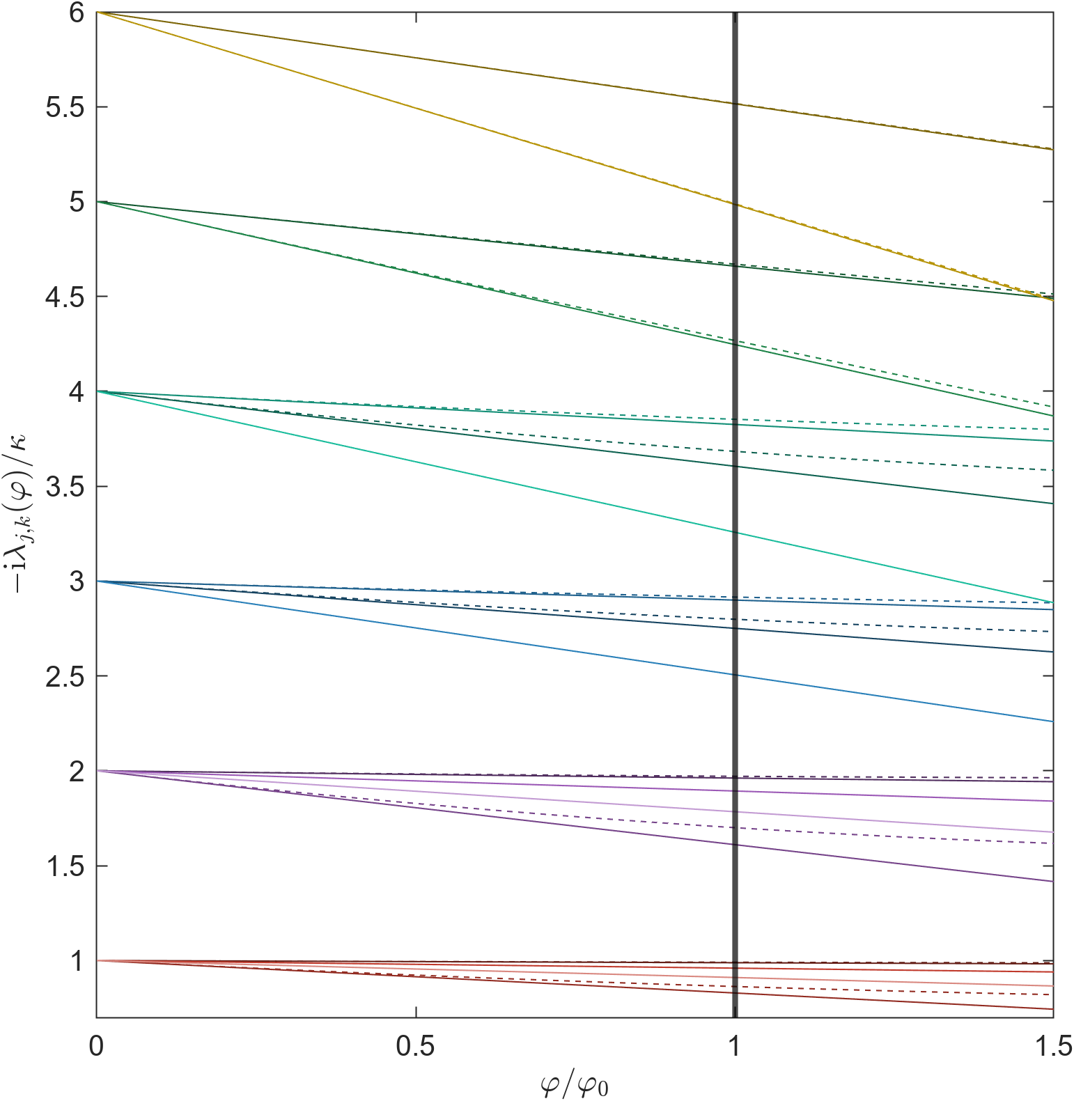
Figure 2: Corrected eigenvalues of $\hat{A}$ corresponding to the degenerate subspaces of $\hat{A}_{0}$, as a function of $\varphi$. The horizontal axis is scaled by $\varphi_{0}=-\frac{\beta}{12}(\frac{\kappa}{2})^{4}$. The solid and dashed lines correspond to the $\mathcal{O}(\varphi)$ and $\mathcal{O}(\varphi^{2})$ corrections respectively. Curves of matching hue (and diverging from the same point at $\varphi=0$) correspond to the same degenerate subspace. This particular set of eigenvalues is for $N=8$.

5.4 Eigenvectors of $\hat{A}$

From Appendix A.2 the eigenvectors of $\bm{\mathsf{A}}$ are expressed as the power series

$$\bm{\psi}_{j,k}(\varphi)=\bm{\psi}_{j,k}^{(0)}+\varphi\bm{\psi}_{j,k}^{(1)}+\mathcal{O}(\varphi^{2}).$$ (58)

The first order correction $\bm{\psi}_{j,k}^{(1)}$ takes the form

$$\bm{\psi}_{j,k}^{(1)}=\sum_{m\neq j}^{M}\frac{{\bm{\psi}_{m}^{(0)}}^{\dagger}\cdot\bm{\mathsf{A}}_{4}\bm{\psi}_{j,k}^{(0)}}{\lambda_{m}^{(0)}-\lambda_{j}^{(0)}}\left(\sum_{l\neq k}^{d_{j}}\frac{{\bm{\psi}_{j,l}^{(0)}}^{\dagger}\cdot\bm{\mathsf{A}}_{4}\bm{\psi}_{m}^{(0)}}{\lambda_{j,l}^{(1)}-\lambda_{j,k}^{(1)}}\bm{\psi}_{j,l}^{(0)}-\bm{\psi}_{m}^{(0)}\right).$$ (59)

As in Section 4.2, we can transform the eigenvectors of $\bm{\mathsf{A}}$ into eigenfunctions of $\hat{A}$ by taking their contraction with the reference vector, $\mathbf{u}$. We have

$$\psi_{j,k}(q,p;\varphi)=\mathbf{u}^{\dagger}\cdot\bm{\psi}_{j,k}(\varphi).$$ (60)

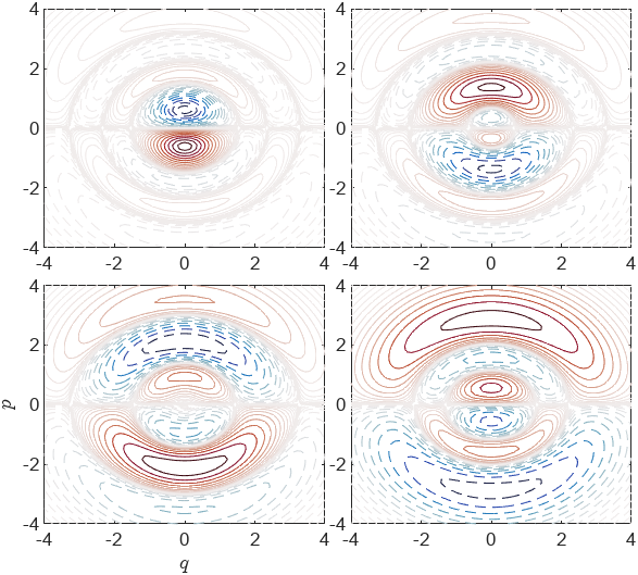
Figure 3: Approximate eigenfunctions of $\hat{A}$, denoted $\psi_{j,k}(q,p;\varphi)$, associated with the $\lambda^{(0)}_{j}=-\mathrm{i}\kappa$ degenerate subspace (bending mode). These are specified by equations 59 and 60. Going from left to right and top to bottom, the panels are sorted from fastest to slowest rate of rotation. We show only the real part of each, noting that the imaginary parts in this case differ only by a rotation. This particular set of eigenfunctions is for $N=8$.

We show in Fig. 3 an example set of $\hat{A}$ eigenfunctions associated with $\lambda_{j}^{(0)}=-\mathrm{i}\kappa$. As discussed in Section 4.2, this is the eigenvalue that controls the rotation of the simple bending mode in Fig. 1. The $\hat{A}$ eigenfunctions contain more sign changes along a radial path from the origin than those of the harmonic oscillator. This facilitates a segmenting of phase space density with distance from the origin (proportional to the action in this case). Each of these structures possesses a different orbital frequency, corresponding to the four diverging solid red lines starting at $-\mathrm{i}\lambda_{j,k}(\varphi)/\kappa=1$ in Fig. 2. The relative spacing of these lines determines the relative rates of rotation. The combination of these two factors causes differential rotation in the distribution function, producing the spiral structure characteristic of phase mixing. The same general idea applies to the other degenerate subspace eigenfunctions, although there are more complicated structures present in the larger $|\lambda_{j}^{(0)}|$ eigenfunctions.

5.5 Dynamics of $f$ from $\hat{A}$

With an estimated spectrum of the full generator, $\hat{A}$, we can compute the distribution function at time $t$. Separating the sum in equation 25 into the distinct contributions from our perturbative analysis we have

$$\hat{S}^{t}f(q,p)=\hat{S}_{0}^{t}f(q,p)\ + \sum_{j=1}^{M-D}\langle\psi_{j},f\rangle\psi_{j}(q,p;\varphi)\mathrm{e}^{\lambda_{j}^{\dagger}(\varphi)t}$$ (61)

$$+\sum_{j}^{D} \sum_{k=1}^{d_{j}}\langle\psi_{j,k},f\rangle\psi_{j,k}(q,p;\varphi)\mathrm{e}^{\lambda_{j,k}^{\dagger}(\varphi)t}.$$

On the right hand side from left to right these are, the harmonic oscillator solution, the non-degenerate subspace of the spectrum of $\hat{A}$, and the total contribution from the $D$ degenerate subspaces.

In Fig. 4, we show three snapshots of $\hat{S}^{t}f$ for three values of $N$. The initial condition is $f_{0}(q,p+\delta p)$, with $\delta p=0.3$, which results in the development of a one-armed spiral. Formation of this structure is driven by the final contribution to equation 61, summing over the split eigenvalues.

Resolvability of spatial structure increases with $N$, which prescribes the representation scale. This can be observed in the progression of contour behavior in the columns of Fig. 4 going from left to right. The number of eigenvalues, and their multiplicities in the $\hat{A}_{0}$ spectrum also increases with $N$. The multiplicities of for example, $\lambda_{j}^{(0)}=-\mathrm{i}\kappa$, are $d_{j}=5,6,7$ for $N=10,12,14$. The higher the multiplicity, the more segmented the frequency content of the solution becomes. The length scale set by $N$ determines which structures can be well represented by the basis regardless of $t$. The fanning out in frequency shown in Fig. 2 coupled with the form of the $\psi_{j,k}$ determines the resolvability of spatiotemporal structure. That is, even if an order $N$ basis is sufficient to represent a state at some $t_{1}$, it is the multiplicity and subsequent splitting of the eigenvalues that dictates the evolution to $t_{2}$. This is most easily seen by comparison $N=12$ and $N=14$ going from $(2\pi)^{-1}\kappa t_{1}=5$ to $(2\pi)^{-1}\kappa t_{2}=8$. At $t_{1}$, the two representations of $f$ are quite similar, but at $t_{2}$, the $N=12$ $f$ does not form the the monotonic density gradient we see along the tail of the spiral in $N=14$, despite not obviously requiring a higher polynomial order.

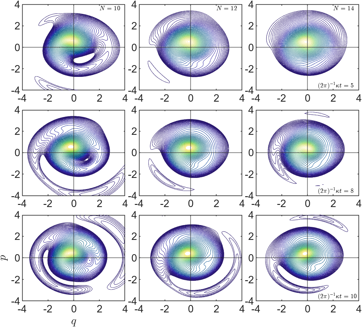
Figure 4: Snapshots of the distribution function $\hat{S}^{t}f$, computed from equation 61. From left to right, $N=10,12,14$. From top to bottom, $(2\pi)^{-1}\kappa t=5,8,10$. In all panels, the $j$th contour value is given by $\mathrm{max}\{f_{0}\}\mathrm{e}^{-\frac{\beta}{2}x_{j}^{2}}$, with $x_{j}=3j/50$. The contour color transitions from yellow to blue with increasing $j$.

6 Discussion

The resolvability of structure in $f$ depends on its representation, or means of observation. When one chooses a number of particles in an $N$-body simulation, a grid resolution in an equation solver, or a finite dimensional basis, a scale is imposed. In this work, we aimed to highlight the relationship between imposed length scale from dimension of representation, and multiplicity of eigenvalues in the spectrum of $\hat{A}_{0}$. Further, that in such a case splitting of the degenerate eigenvalues by $\hat{A}_{4}$ drives mixing in $f$.

For the spectrum of $\hat{A}_{0}$, the number of unique degenerate eigenvalues, and their average multiplicity increases with $M$, the size of the basis. In this construction, spiral formation is achieved through a linear combination of structures that span the entire $(q,p)$ plane (Fig. 3). This is in contrast to the picture described in Section 1, in which essentially every infinitesimal annulus of phase space volume at a different radius from the origin orbits with a different frequency. In Banik et al. (2022), phase mixing is achieved through a linear response term of the form $\mathrm{e}^{in(\theta-\Omega(I)t)}$, where $(\theta,I)$ are angle-action coordinates, and $\Omega$ is the oscillatory frequency of the orbits. Since the frequencies depends on the actions, orbits at different actions will possess varying frequencies, leading to deformation of $f$.

One could suppose that for an infinite dimensional basis, $f$ decomposes into an infinite set of delta functions of $q$ and $p$, each nonzero at a different point in the plane. In this case, all of the different packets of phase space density may have different orbital frequencies, and we obtain the original picture of the process, essentially moving to a discrete particle representation. Given the premise of increasing dimension corresponding to increasing degeneracy of the eigenvalues, we suppose that in the limit case of a an infinite dimensional representation, the discretely split degenerate eigenvalues may become the continuous bands described in Mathur (1990) and Weinberg (1991).

The analysis here omits a self-interaction potential. This means that $\hat{A}$ does not depend on $t$, and the integral in equation 22 is trivial. Were this not the case, the operator solution $\hat{U}^{t}$ would take the form of a Dyson series, obtained by iterative solution of the implicit equation $\hat{U}^{t}=1+\int_{0}^{t}d\tau\hat{A}(\tau)\hat{U}^{\tau}$ (Sakurai & Napolitano, 2017). In doing this, it would be sensible to separate the self-interaction contribution to the Hamiltonian, and parameterize its strength with for example, $\alpha$. Computing the necessary Dyson series to some order in $\alpha$ is technically possible. The main constraint is that the matrix element integrals cannot necessarily be evaluated analytically for a non-polynomial potential in our chosen basis. Using the exact one-dimensional Green’s function of the Poisson equation poses a challenge in this regard. One option is to adopt a Hamiltonian Mean Field (HMF) approach as in Inagaki & Konishi (1993), replacing the absolute value function with a polynomial that preserves some desired properties. In this case, the self-interaction can be expressed in terms of the moments of $f$ as in Section 4.3, which work nicely with the functional formalism used here. The simplest case would be a quadratic interaction, $v(q,q^{\prime})\propto(q-q^{\prime})^{2}$. Here, the self-interaction is a quadratic potential well that tracks the expectation value of position with respect to $f$, which is the moment $\hat{U}^{t}F_{1,0}$.

7 Conclusions

We have described a procedure for determining the CBE dynamics of $f$, by mapping the problem into a set of functionals $G[f]$ which satisfy a Schrödinger-type equation. To calculate explicit matrix representations of operators, we adopted a finite dimensional set of basis functions that impose a minimum length scale on $f$. For an illustrative example of phase mixing, we treated a quartic potential perturbatively with respect to a harmonic oscillator solution. We observed that the algebraic multiplicity of harmonic oscillator eigenvalues increases with dimension of the finite basis representation. Subsequently, we showed that the anharmonic potential splits the degenerate eigenvalues, creating the amplitude dependent frequencies characteristic of phase mixing.

Determining the spectrum of $\hat{A}$ constitutes a form of PCA. Rather than inferring important structures from time-series data, we are identifying those structures with respect to a system model (presupposed potential), independent of initial conditions. Knowing analytic functions of $q$ and $p$ that are instrumental in the formation and evolution of spirals presents an avenue for hypothesis testing with observational data. In principle, a kinematic snapshot can be projected onto a basis determined in this way. One can imagine then devising a likelihood function to compare eigenbases given the data to probe the Galactic potential. This is a similar notion to that described in Darling & Widrow (2021), where a statistical model is used to determine the most likely eigenfunctions and eigenvalues given a snapshot.

It is also of interest to further investigate the scale-dependent mixing process studied here in the context of other work around coarse-grained evolution of the CBE, as in Chavanis et al. (1996) or Chavanis, P. H. & Bouchet, F. (2005). In the latter, one of the definitions of a coarse-grained $f$ is a windowed functional. That is, $f$ is taken in convolution with some kernel that sets the representation scale. Preliminary work suggests that the equation of motion in that case is equivalent to equation 20 up to a diffusion current term.

Data Availability

Calculations were carried out in MATLAB. Custom software used for this paper is available upon reasonable request. Colormaps used in contour plots are thanks to Thyng et al. (2016).

Appendix A Perturbative treatment of degenerate eigenvalues

We aim to find eigenvectors $\bm{\psi}_{j,k}(\varphi)$ and eigenvalues $\lambda_{j,k}(\varphi)$ that satisfy the perturbed eigenvalue problem

$$\left(\bm{\mathsf{A}}_{\mathsf{0}}+\varphi\bm{\mathsf{A}}_{\mathsf{4}}\right)\bm{\psi}_{j,k}=\lambda_{j,k}\bm{\psi}_{j,k}.$$ (62)

This is achieved by assuming a power series in $\varphi$ for both quantities,

$$\lambda_{j,k}(\varphi) =\lambda_{j,k}^{(0)}+\varphi\lambda_{j,k}^{(1)}+\mathcal{O}(\varphi^{2}),$$ (63)

$$\bm{\psi}_{j,k}(\varphi) =\bm{\psi}_{j,k}^{(0)}+\varphi\bm{\psi}_{j,k}^{(1)}+\mathcal{O}(\varphi^{2}).$$

This requires that both the eigenvectors and eigenvalues vary smoothly with respect to change in the perturbation parameter $\varphi$. Since the eigenvalues are scalar, this is the case by default. We assure a smooth variation in the eigenvectors by the procedure described in Section 5.3.1.

Substituting the assumed power series into equation 62, and equating terms of equal power in $\varphi$, one finds a set of equations. Those corresponding to the first three powers of $\varphi$ are,

$$\left(\bm{\mathsf{A}}_{0}-\lambda_{j}^{(0)}\right)\bm{\psi}_{j,k}^{(0)} =0,$$ (64)

$$\left(\bm{\mathsf{A}}_{0}-\lambda_{j}^{(0)}\right)\bm{\psi}_{j,k}^{(1)} =\left(\lambda^{(1)}_{j,k}-\bm{\mathsf{A}}_{4}\right)\bm{\psi}_{j,k}^{(0)},$$

$$\left(\bm{\mathsf{A}}_{0}-\lambda_{j}^{(0)}\right)\bm{\psi}^{(2)}_{j,k} =\left(\lambda_{j,k}^{(1)}-\bm{\mathsf{A}}_{4}\right)\bm{\psi}_{j,k}^{(1)}+\lambda_{j,k}^{(2)}\bm{\psi}_{j,k}^{(0)}.$$

A.1 Degenerate case: eigenvalues

To determine the first order correction to the eigenvalues, we begin by contracting the $\mathcal{O}(\varphi)$ case (second line) in equation 64 with ${\bm{\psi}^{(0)}_{j,l}}^{\dagger}$. That is

$${\bm{\psi}^{(0)}_{j,l}}^{\dagger}\cdot\left(\bm{\mathsf{A}}_{0}-\lambda_{j}^{(0)}\right)\bm{\psi}_{j,k}^{(1)}={\bm{\psi}^{(0)}_{j,l}}^{\dagger}\cdot\left(\lambda^{(1)}_{j,k}-\bm{\mathsf{A}}_{4}\right)\bm{\psi}_{j,k}^{(0)}.$$ (65)

Since ${\bm{\psi}^{(0)}_{j,k}}^{\dagger}$ is a left-eigenvector of $\bm{\mathsf{A}}_{0}$, ${\bm{\psi}^{(0)}_{j,k}}^{\dagger}\bm{\mathsf{A}}_{0}=\lambda_{j,k}^{(0)}{\bm{\psi}^{(0)}_{j,k}}^{\dagger}$, and the left hand side is zero. We are left with

$$\lambda_{j,k}^{(1)}{\bm{\psi}^{(0)}_{j,l}}^{\dagger}\cdot\bm{\psi}_{j,k}^{(0)}={\bm{\psi}^{(0)}_{j,l}}^{\dagger}\cdot\bm{\mathsf{A}}_{4}\bm{\psi}_{j,k}^{(0)}.$$ (66)

Since ${\bm{\psi}^{(0)}_{j,l}}^{\dagger}\cdot\bm{\psi}_{j,k}^{(0)}=\delta_{l}^{k}$, equation 66 then reduces to

$$\lambda_{j,k}^{(1)}={\bm{\psi}^{(0)}_{j,k}}^{\dagger}\cdot\bm{\mathsf{A}}_{4}\bm{\psi}_{j,k}^{(0)}.$$ (67)

That is, the $\mathcal{O}(\varphi)$ corrections to the degenerate eigenvalues are the diagonal entries of the perturbation, $\bm{\mathsf{A}}_{4}$, when it is projected onto the degenerate subspace corresponding to $\lambda^{(0)}_{j,k}$. In other words, if we project $\bm{\mathsf{A}}_{4}$ onto a degenerate subspace, the eigenvalues of the projected matrix are the first order corrections $\lambda_{j,k}^{(1)}$.

A.2 Degenerate case: eigenvectors

In general, the eigenvectors of $\bm{\mathsf{A}}$ may contain components from the entire space, including vectors from both in and not in the degenerate subspace. That is, we want to know how to project $\bm{\psi}_{j,k}^{(1)}$ onto the sets of $\bm{\psi}_{j}^{(0)}$ and $\bm{\psi}_{j,k}^{(0)}$. It follows that we can do this if we have general expressions for both of the contractions, ${\bm{\psi}_{j}^{(0)}}^{\dagger}\cdot\bm{\psi}_{j,k}^{(1)}$ and ${\bm{\psi}_{j,k}^{(0)}}^{\dagger}\cdot\bm{\psi}_{j,k}^{(1)}$.

We will treat both cases separately, first computing the contribution from the subset of the complete basis that excludes the degenerate subspace. We begin by contracting the first order case in equation 64 with ${\bm{\psi}_{j}^{(0)}}^{\dagger}$. We have

$${\bm{\psi}_{l}^{(0)}}^{\dagger}\cdot\left(\bm{\mathsf{A}}_{0}-\lambda_{j}^{(0)}\right)\bm{\psi}_{j,k}^{(1)}={\bm{\psi}_{l}^{(0)}}^{\dagger}\cdot\left(\lambda^{(1)}_{j,k}-\bm{\mathsf{A}}_{4}\right)\bm{\psi}_{j,k}^{(0)}.$$ (68)

Similar to when we computed the eigenvalue correction, we note that ${\bm{\psi}_{j}^{(0)}}^{\dagger}\bm{\mathsf{A}}_{0}=\lambda_{j}^{(0)}{\bm{\psi}_{j}^{(0)}}^{\dagger}$. Additionally, we know that ${\bm{\psi}_{l}^{(0)}}^{\dagger}$ and $\bm{\psi}_{j,k}^{(0)}$ are orthogonal for all $l,j,k$, since one of them is within the degenerate subspace and the other is not. From these two arguments, we can simplify equation 68 to

$${\bm{\psi}_{l}^{(0)}}^{\dagger}\cdot\bm{\psi}_{j,k}^{(1)}=\frac{{\bm{\psi}_{l}^{(0)}}^{\dagger}\cdot\bm{\mathsf{A}}_{4}\bm{\psi}_{j,k}^{(0)}}{\lambda_{l}^{(0)}-\lambda_{j}^{(0)}}.$$ (69)

For the degenerate subset contribution, we do not get any new information by attempting a contraction of ${\bm{\psi}_{j,k}^{(0)}}^{\dagger}$ with the first order case in equation 64. Let us instead try the $\mathcal{O}(\varphi^{2})$ equation. We take

$${\bm{\psi}_{j,l}^{(0)}}^{\dagger}\cdot\left(\bm{\mathsf{A}}_{0}-\lambda_{j}^{(0)}\right)\bm{\psi}^{(2)}_{j,k}={\bm{\psi}_{j,l}^{(0)}}^{\dagger}\cdot\left(\lambda_{j,k}^{(1)}-\bm{\mathsf{A}}_{4}\right)\bm{\psi}_{j,k}^{(1)}$$ (70)

$$+\lambda_{j,k}^{(2)}{\bm{\psi}_{j,l}^{(0)}}^{\dagger}\cdot\bm{\psi}_{j,k}^{(0)}.$$

Note that we use the same index $j$ on the first index for the introduced vector, as if we allowed for a different index, we would be considering the case that one degenerate subspace is projected onto another. All of the distinct subspaces are orthogonal, so this can only result in zero.

We can proceed by again noting that ${\bm{\psi}_{j,l}^{(0)}}^{\dagger}\bm{\mathsf{A}}_{0}=\lambda_{j,l}^{(1)}$. Since $\lambda_{j,l}=\lambda_{j}\ \forall\ l$, the left hand side is zero. Further, ${\bm{\psi}_{j,l}^{(0)}}^{\dagger}\cdot\bm{\psi}_{j,k}^{(0)}=\delta_{l}^{k}$, so we are are left with

$$\lambda_{j,k}^{(2)}\delta_{l}^{k}=-{\bm{\psi}_{j,l}^{(0)}}^{\dagger}\cdot\left(\lambda_{j,k}^{(1)}-\bm{\mathsf{A}}_{4}\right)\bm{\psi}_{j,k}^{(1)}.$$ (71)

Of course, we do not know $\bm{\psi}_{j,k}^{(1)}$, as that is what we are trying to determine here. We do know however that it can have contributions from $\bm{\psi}_{j}^{(0)}$ and $\bm{\psi}_{j,l}^{(0)}$. Let us suppose that it takes the form

$$\bm{\psi}_{j,k}^{(1)}=\sum_{m\neq j}^{M}\left({\bm{\psi}_{m}^{(0)}}^{\dagger}\cdot\bm{\psi}_{j,k}^{(1)}\right)\bm{\psi}_{m}^{(0)}+\sum_{l}^{d_{j}}\left({\bm{\psi}_{j,l}^{(0)}}^{\dagger}\cdot\bm{\psi}_{j,k}^{(1)}\right)\bm{\psi}_{j,l}^{(0)}.$$ (72)

We have already found what we need to express the first sum explicitly in equation 69. With this, we may write

$$\bm{\psi}_{j,k}^{(1)}=\sum_{m\neq j}^{M}\frac{{\bm{\psi}_{m}^{(0)}}^{\dagger}\cdot\bm{\mathsf{A}}_{4}\bm{\psi}_{j,k}^{(0)}}{\lambda_{m}^{(0)}-\lambda_{j}^{(0)}}\bm{\psi}_{m}^{(0)}+\sum_{l}^{d_{j}}\left({\bm{\psi}_{j,l}^{(0)}}^{\dagger}\cdot\bm{\psi}_{j,k}^{(1)}\right)\bm{\psi}_{j,l}^{(0)}.$$ (73)

Continuing with equation 71, we have

$$\lambda_{j,k}^{(2)}\delta_{l}^{k}= -\lambda_{j,k}^{(1)}\sum_{m\neq j}^{M}\frac{{\bm{\psi}_{m}^{(0)}}^{\dagger}\cdot\bm{\mathsf{A}}_{4}\bm{\psi}_{j,k}^{(0)}}{\lambda_{m}^{(0)}-\lambda_{j}^{(0)}}{\bm{\psi}_{j,l}^{(0)}}^{\dagger}\cdot\bm{\psi}_{m}^{(0)}$$ (74)

$$+\sum_{m\neq j}^{M}\frac{{\bm{\psi}_{m}^{(0)}}^{\dagger}\cdot\bm{\mathsf{A}}_{4}\bm{\psi}_{j,k}^{(0)}}{\lambda_{m}^{(0)}-\lambda_{j}^{(0)}}{\bm{\psi}_{j,l}^{(0)}}^{\dagger}\cdot\bm{\mathsf{A}}_{4}\bm{\psi}_{m}^{(0)}$$

$$-\sum_{n}^{d_{j}}\lambda_{j,k}^{(1)}\left({\bm{\psi}_{j,n}^{(0)}}^{\dagger}\cdot\bm{\psi}_{j,k}^{(1)}\right)\left({\bm{\psi}_{j,l}^{(0)}}^{\dagger}\cdot\bm{\psi}_{j,n}^{(0)}\right)$$

$$+\sum_{n}^{d_{j}}\left({\bm{\psi}_{j,n}^{(0)}}^{\dagger}\cdot\bm{\psi}_{j,k}^{(1)}\right){\bm{\psi}_{j,l}^{(0)}}^{\dagger}\cdot\bm{\mathsf{A}}_{4}\bm{\psi}_{j,n}^{(0)}$$

The first term on the right hand side is zero since ${\bm{\psi}_{j,l}^{(0)}}^{\dagger}\cdot\bm{\psi}_{m}^{(0)}$ are orthogonal for $m\neq j$. The sum in the term on the right hand side collapses because ${\bm{\psi}_{j,l}^{(0)}}^{\dagger}\cdot\bm{\psi}_{j,n}^{(0)}=\delta_{l}^{n}$. Making these simplifications leaves us with,

$$\lambda_{j,k}^{(2)}\delta_{l}^{k}= \sum_{m\neq j}^{M}\frac{{\bm{\psi}_{m}^{(0)}}^{\dagger}\cdot\bm{\mathsf{A}}_{4}\bm{\psi}_{j,k}^{(0)}}{\lambda_{m}^{(0)}-\lambda_{j}^{(0)}}{\bm{\psi}_{j,l}^{(0)}}^{\dagger}\cdot\bm{\mathsf{A}}_{4}\bm{\psi}_{m}^{(0)}$$ (75)

$$-\lambda_{j,k}^{(1)}\left({\bm{\psi}_{j,l}^{(0)}}^{\dagger}\cdot\bm{\psi}_{j,k}^{(1)}\right)$$

$$+\sum_{n}^{d_{j}}\left({\bm{\psi}_{j,n}^{(0)}}^{\dagger}\cdot\bm{\psi}_{j,k}^{(1)}\right){\bm{\psi}_{j,l}^{(0)}}^{\dagger}\cdot\bm{\mathsf{A}}_{4}\bm{\psi}_{j,n}^{(0)}.$$

Since the degenerate subspace basis vectors $\bm{\psi}_{j,k}^{(0)}$ are chosen such that they diagonalize $\bm{\mathsf{A}}_{4}$, the only nonzero matrix elements ${\bm{\psi}_{j,l}^{(0)}}^{\dagger}\cdot\bm{\mathsf{A}}_{4}\bm{\psi}_{j,n}^{(0)}$ are those along the diagonal. We may therefore simplify this term as

$$\lambda_{j,k}^{(2)}\delta_{l}^{k}= \sum_{m\neq j}^{M}\frac{{\bm{\psi}_{m}^{(0)}}^{\dagger}\cdot\bm{\mathsf{A}}_{4}\bm{\psi}_{j,k}^{(0)}}{\lambda_{m}^{(0)}-\lambda_{j}^{(0)}}{\bm{\psi}_{j,l}^{(0)}}^{\dagger}\cdot\bm{\mathsf{A}}_{4}\bm{\psi}_{m}^{(0)}$$ (76)

$$-\lambda_{j,k}^{(1)}\left({\bm{\psi}_{j,l}^{(0)}}^{\dagger}\cdot\bm{\psi}_{j,k}^{(1)}\right)+\sum_{n}\lambda_{j,l}^{(1)}\delta_{l}^{n}\left({\bm{\psi}_{j,n}^{(0)}}^{\dagger}\cdot\bm{\psi}_{j,k}^{(1)}\right).$$

Collapsing the sum according to the $\delta_{l}^{n}$ we are left with

$$\lambda_{j,k}^{(2)}\delta_{l}^{k}=\sum_{m\neq j}^{M}\frac{{\bm{\psi}_{m}^{(0)}}^{\dagger}\cdot\bm{\mathsf{A}}_{4}\bm{\psi}_{j,k}^{(0)}}{\lambda_{m}^{(0)}-\lambda_{j}^{(0)}}{\bm{\psi}_{j,l}^{(0)}}^{\dagger}\cdot\bm{\mathsf{A}}_{4}\bm{\psi}_{m}^{(0)}$$ (77)

$$+\left(\lambda_{j,l}^{(1)}-\lambda_{j,k}^{(1)}\right){\bm{\psi}_{j,l}^{(0)}}^{\dagger}\cdot\bm{\psi}_{j,k}^{(1)}.$$

This equation has two cases. First, if $l\neq k$, we obtain the explicit expression for ${\bm{\psi}_{j,l}^{(0)}}^{\dagger}\cdot\bm{\psi}_{j,k}^{(1)}$ that we have been looking for. That is

$${\bm{\psi}_{j,l}^{(0)}}^{\dagger}\cdot\bm{\psi}_{j,k}^{(1)}=\frac{1}{\lambda_{j,l}^{(1)}-\lambda_{j,k}^{(1)}}\sum_{m\neq j}^{M}\frac{{\bm{\psi}_{m}^{(0)}}^{\dagger}\cdot\bm{\mathsf{A}}_{4}\bm{\psi}_{j,k}^{(0)}}{\lambda_{m}^{(0)}-\lambda_{j}^{(0)}}{\bm{\psi}_{j,l}^{(0)}}^{\dagger}\cdot\bm{\mathsf{A}}_{4}\bm{\psi}_{m}^{(0)}.$$ (78)

Taking the case $l=k$ yields the $\mathcal{O}(\varphi^{2})$ correction to the eigenvalues if desired.

Now that we have explicit expressions for both ${\bm{\psi}_{m}^{(0)}}^{\dagger}\cdot\bm{\psi}_{j,k}^{(1)}$ and ${\bm{\psi}_{j,l}^{(0)}}^{\dagger}\cdot\bm{\psi}_{j,k}^{(1)}$ we can express the first order corrections to the eigenvectors of $\bm{\mathsf{A}}_{4}$ as we had outlined in equation 72.

$$\bm{\psi}_{j,k}^{(1)}= -\sum_{m\neq j}^{M}\frac{{\bm{\psi}_{m}^{(0)}}^{\dagger}\cdot\bm{\mathsf{A}}_{4}\bm{\psi}_{j,k}^{(0)}}{\lambda_{m}^{(0)}-\lambda_{j}^{(0)}}\bm{\psi}_{m}^{(0)}$$ (79)

$$+\sum_{l\neq k}^{d_{j}}\frac{1}{\lambda_{j,l}^{(1)}-\lambda_{j,k}^{(1)}}\sum_{m\neq j}^{M}\frac{{\bm{\psi}_{m}^{(0)}}^{\dagger}\cdot\bm{\mathsf{A}}_{4}\bm{\psi}_{j,k}^{(0)}}{\lambda_{m}^{(0)}-\lambda_{j}^{(0)}}\left({\bm{\psi}_{j,l}^{(0)}}^{\dagger}\cdot\bm{\mathsf{A}}_{4}\bm{\psi}_{m}^{(0)}\right)\bm{\psi}_{j,l}^{(0)}.$$

Factoring, this can be written more compactly as equation 59.

References

- Abel et al. (2012) Abel T., Hahn O., Kaehler R., 2012, MNRAS, 427, 61
- Antoja et al. (2018) Antoja T., et al., 2018, Nature, 561, 360
- Arnold (1989) Arnold V., 1989, Mathematical methods of classical mechanics. Vol. 60, Springer
- Banik et al. (2022) Banik U., Weinberg M. D., van den Bosch F. C., 2022, ApJ, 935, 135
- Bennett & Bovy (2018) Bennett M., Bovy J., 2018, Monthly Notices of the Royal Astronomical Society, 482, 1417
- Bennett & Bovy (2021) Bennett M., Bovy J., 2021, Monthly Notices of the Royal Astronomical Society, 503, 376
- Binney & Tremaine (2008) Binney J., Tremaine S., 2008, Galactic Dynamics: Second Edition. Princeton University
- Chavanis, P. H. & Bouchet, F. (2005) Chavanis, P. H. Bouchet, F. 2005, A&A, 430, 771
- Chavanis et al. (1996) Chavanis P. H., Sommeria J., Robert R., 1996, The Astrophysical Journal, 471, 385
- Conway (1994) Conway J., 1994, A Course in Functional Analysis. Graduate Texts in Mathematics, Springer New York
- Darling & Widrow (2019a) Darling K., Widrow L. M., 2019a, MNRAS, 484, 1050
- Darling & Widrow (2019b) Darling K., Widrow L. M., 2019b, MNRAS, 490, 114
- Darling & Widrow (2021) Darling K., Widrow L. M., 2021, MNRAS, 506, 3098
- Gaia Collaboration et al. (2018) Gaia Collaboration et al., 2018, AAP, 616, A11
- Griffiths & Schroeter (2018) Griffiths D. J., Schroeter D. F., 2018, Introduction to Quantum Mechanics, 3 edn. Cambridge University Press
- Hunt et al. (2021) Hunt J. A. S., Stelea I. A., Johnston K. V., Gandhi S. S., Laporte C. F. P., Bédorf J., 2021, Monthly Notices of the Royal Astronomical Society, 508, 1459
- Inagaki & Konishi (1993) Inagaki S., Konishi T., 1993, PASJ, 45, 733
- Johnson et al. (2023) Johnson A. C., Petersen M. S., Johnston K. V., Weinberg M. D., 2023, MNRAS, 521, 1757
- Koopman (1931) Koopman B. O., 1931, Proceedings of the National Academy of Sciences, 17, 315
- Kutz et al. (2016) Kutz J. N., Brunton S. L., Brunton B. W., Proctor J. L., 2016, Dynamic Mode Decomposition: Data-Driven Modeling of Complex Systems. SIAM
- Mathur (1990) Mathur S. D., 1990, MNRAS, 243, 529
- Mezić (2005) Mezić I., 2005, Nonlinear Dynamics, 41, 309
- Morrison (1980) Morrison P. J., 1980, ] 10.2172/6825879
- Nakao & Mezić (2020) Nakao H., Mezić I., 2020, Chaos, 30, 113131
- Perez (2005) Perez J., 2005, Transport Theory and Statistical Physics, 34, 391
- Perrett et al. (2003) Perrett K. M., Stiff D. A., Hanes D. A., Bridges T. J., 2003, ApJ, 589, 790
- Rowley et al. (2009) Rowley C. W., Mezic I., Bagheri S., Schlatter P., Henningson D. S., 2009, Journal of Fluid Mechanics, 641, 115–127
- Sakurai & Napolitano (2017) Sakurai J. J., Napolitano J., 2017, Modern Quantum Mechanics, 2 edn. Cambridge University Press, doi:10.1017/9781108499996
- Schönrich & Binney (2018) Schönrich R., Binney J., 2018, MNRAS, 481, 1501
- Sethna (2006) Sethna J. P., 2006, Statistical Mechanics: Entropy, Order Parameters and Complexity, first edition edn. Oxford University Press, Great Clarendon Street, Oxford OX2 6DP
- Thyng et al. (2016) Thyng K. M., Greene C. A., Hetland R. D., Zimmerle H. M., DiMarco S. F., 2016, Oceanography, 29, 9
- Tremaine (1999) Tremaine S., 1999, Monthly Notices of the Royal Astronomical Society, 307, 877
- Weinberg (1991) Weinberg M. D., 1991, ApJ, 373, 391
- Weinberg & Petersen (2021) Weinberg M. D., Petersen M. S., 2021, MNRAS, 501, 5408