The Cosmic Neutrino Background

Abstract

The cosmic neutrino background is like the cosmic microwave background, but less photon-y and more neutrino-ey. The CNB is also less talked about than the CMB, mostly because it’s nearly impossible to detect directly. But if it could be detected, it would be interesting in several ways that are discussed.

1 $\nu$ overview (or ‘news’)

Let’s start by giving an overview of the relevant properties of neutrinos:

• neutrinos are hard to detect;

• they come in 3 flavours, which can mix;

• we don’t know why the flavour and mass states are so messed up (unlike the situation for quarks);

• we don’t know if they’re their own anti-particles or not (Majorana versus Dirac);

• we don’t know their masses, or even if they have the “normal hierarchy” ($m_{3}\gg m_{2}\mathrel{\hbox to0.0pt{\lower 3.0pt\hbox{$\mathchar 536\relax$}\hss}\raise 2.0pt\hbox{$\mathchar 318\relax$}}m_{1}$) or an “inverted hierarchy” ($m_{2}\mathrel{\hbox to0.0pt{\lower 3.0pt\hbox{$\mathchar 536\relax$}\hss}\raise 2.0pt\hbox{$\mathchar 318\relax$}}m_{1}\gg m_{3}$).

And let’s also summarise some information for cosmological neutrinos (making informal comments as notes among the references at the end, like this one [1]):

• cosmological neutrinos are really hard to detect;

• there are about 340 for every cm³ of the Universe (making them the second most common particle, after photons);

• if we could detect them, they’d tell us interesting things;

• the sum of neutrino masses is expected to be the 7th (or 8th) cosmological parameter.

This last point is why many cosmologists are currently excited about neutrinos. There is a very strong expectation that soon it will be possible to make a measurement of the sum of the neutrino masses, $\sum m_{\nu}$, because of the effects of the cosmic neutrino background (CNB or C$\nu$B) on cosmological power spectra, after the neutrinos become non-relativistic. The standard cosmological model, also known as $\Lambda$CDM (or “cosmological-constant-dominated, cold dark matter”), has six basic parameters, or seven if we include the amplitude of the photon background. The mass density of neutrinos in the CNB will be one additional parameter.

For a good summary of neutrinos in cosmology, I recommend the review article by Julien Lesgourgues and Licia Verde in the “Particle Data Book” (PDG) [2]. What follows will be a broad discussion of the cosmic neutrino background (CNB or C$\nu$B), from the perspective of someone who has worked on the photon background, and would love to live in a universe where it was routine to extract information from the CNB, just as it is now for the CMB. This will not be a particle-physics-oriented overview – for more on the particle properties of neutrinos I would suggest reading the PDG review by Maria Gonzalez-Garcia and Masashi Yokoyama [3]). However, it will be important to consider how neutrinos differ from photons, which of course involves some particle physics [4].

2 $\nu$ cosmic background

As already stated, neutrinos are hard to detect, even if they’re produced copiously in the early Universe and other sources. The Sun makes so many neutrinos that even at the distance of the Earth, something like $10^{15}$ of them enter your body every second [5], and the same number also exit your body every second. There’s a small chance that one of them might interact with you in your lifetime. Human bodies are of course not very sensitive detectors, and we can do much better with a tailor-made experiment, but nevertheless, the numbers detected are only measured in the tens per day. Solar neutrinos are typically at energies in the MeV range. What we’re focussing on in this article are the CNB neutrinos, which are also at “em-ee-vee” energies, but now it’s meV rather than MeV. Such low-energy neutrinos basically don’t interact with anything [6].

The neutrinos of the CNB were made at very early times, before the weak interactions froze out. We can calculate their number density today, which turns out to be about $340\,{\rm cm}^{-3}$ for all flavours together (and including anti-neutrinos). That’s only slightly less than the value $411\,{\rm cm}^{-3}$ for the photons of the CMB. This makes neutrinos the second most populous particle in the Universe (if we don’t count gravitons from inflation, at least [7]). In terms of mass density, the fraction of the cosmological critical density in massive neutrinos is

$$\Omega_{\nu}={\sum m_{\nu}\over 93.14\,h^{2}\,{\rm eV}},$$ (1)

where the Hubble parameter is $H_{0}=100\,h\,{\rm km}\,{\rm s}^{-1}\,{\rm Mpc}^{-1}$ and $h^{2}\simeq 0.5$. If we assume the minimal value for the sum of the neutrino masses (about $0.06\,$eV, which comes from adopting the normal hierarchy and using estimates of the mass-squared differences from neutrino oscillation measurements), then we find that $\Omega_{\nu}\simeq 0.0014$. This can be compared with the contributions from baryons and cold dark matter, $\Omega_{\rm b}=0.049$ and $\Omega_{\rm c}=0.261$, respectively [8, 9].

On the other hand, the estimated cosmic density of stars in an average piece of the Universe is $\Omega_{\ast}\simeq 0.0015$ [10]. This means that $\Omega_{\nu}\simeq\Omega_{\ast}$ [11, 12], which is of course just a coincidence [13], but the reason to point it out is that it emphasises that the neutrinos are not negligible, and some of the dark matter consists of neutrinos. It has been a pretty good approximation up until now to ignore the effects of neutrino mass on structure formation, but as measurements become more precise, then eventually we’re not going to be able to neglect the neutrinos. We’re now at the point where the neutrinos need to be taken into account for the next generation of surveys.

Another way of saying the same thing is that if the neutrinos were a lot more massive, then they would be the ideal dark matter candidates. They are already known to exist, are everywhere in the Cosmos and have no electromagnetic interactions. In some ways it’s unfortunate that nature didn’t give us more massive neutrinos – but we now know that their masses are small enough that the fraction of dark matter that is neutrinos is almost (but not completely) negligible and instead we need the dark matter to be an unknown particle that also has very weak interactions [14].

3 $\nu$ background versus photon backgrounds

Let’s delve a bit more deeply into the CNB, by first having a closer look at the cosmic photon backgrounds. There’s a long history of considering the measurement and modelling of the emission from the extragalactic Universe, spanning all wavelengths in the electromagnetic spectrum. Figure 1 shows some examples of reviews of this topic. The earliest is probably that of Longair & Sunyaev in 1971 [15], who, despite having very limited empirical data at that time, got things astonishingly correct! A significant advance was made in 1990, when Ressell & Turner presented the “Grand Unified Photon Spectrum” [16]. This compilation was updated (by me) and published in conference proceedings in 1999 [17, 18, 19], as well as in Chapter 26 of “Allen’s Astrophysical Quantities” [20]. This built on Ted Ressell’s use of upper limits [21] to also include lower limits from source counts, in order to bracket the measurements. A more detailed review of constraints on the infrared (IR) part of the background was published by Dole, Lagache, Puget and collaborators in several articles around 2006 [22, 23] – the last panel in Fig. 1 shows the IR and optical parts of the background [24].

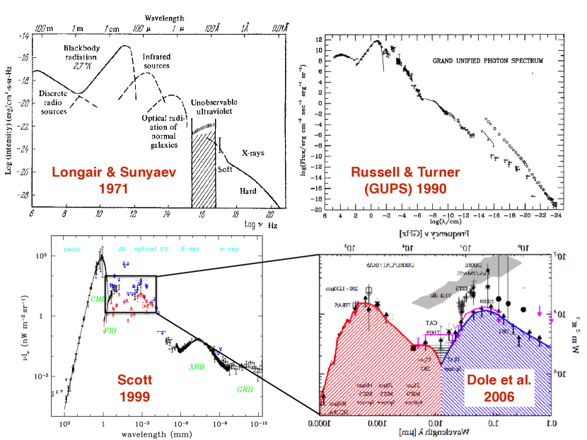
Figure 1: Collection of historical compilations of observational constraints on the extragalactic photon background. The lower-left panel multiplies the vertical axis by one more power of frequency, to give a better comparison of the energy densities in various components. The lower-right panel focuses on the far-IR and optical backgrounds coming from stars.

The largest fraction of the total photon energy density is the CMB, thermal radiation from the early Universe. The optical and near-IR portion is dominated by direct starlight, while the far-IR part traces the starlight absorbed and reradiated by interstellar dust. Higher energy photons come mostly from active galactic nuclei (AGN) of various types. In general, the extragalactic photon background intensity that we measure is an integral of the history of the photon luminosity density, ${\cal L}(z)$ of sources over all redshifts:

$$I=\left({c\over 4\pi}\right)\int_{0}^{\infty}{\cal L}(z)\left|{dt\over dz}\right|{dz\over 1+z}.$$ (2)

Thus, the background tells us about the history of star formation, heavy-element production, black hole accretion, etc.

The origin of various parts of the photon spectrum is labelled on a recent compilation of the “Spectrum of the Universe” by Hill, Masui & Scott [25] in Fig. 2. This “splatter” diagram combines data in each wavelength range, making a wide splash of colour where the uncertainties are large and a thin line where the data are more precise [26]. A similar exercise can be performed for extragalactic neutrinos – except of course the data are mostly non-existent. Still, we can estimate what the cosmic neutrino spectrum would look like. The best attempt to do this is in a review by Vitagliano, Tamborra & Raffelt [27]. These authors summarise backgrounds coming from sources on the Earth, the Sun, our Galaxy and distant galaxies, in addition to the CNB.

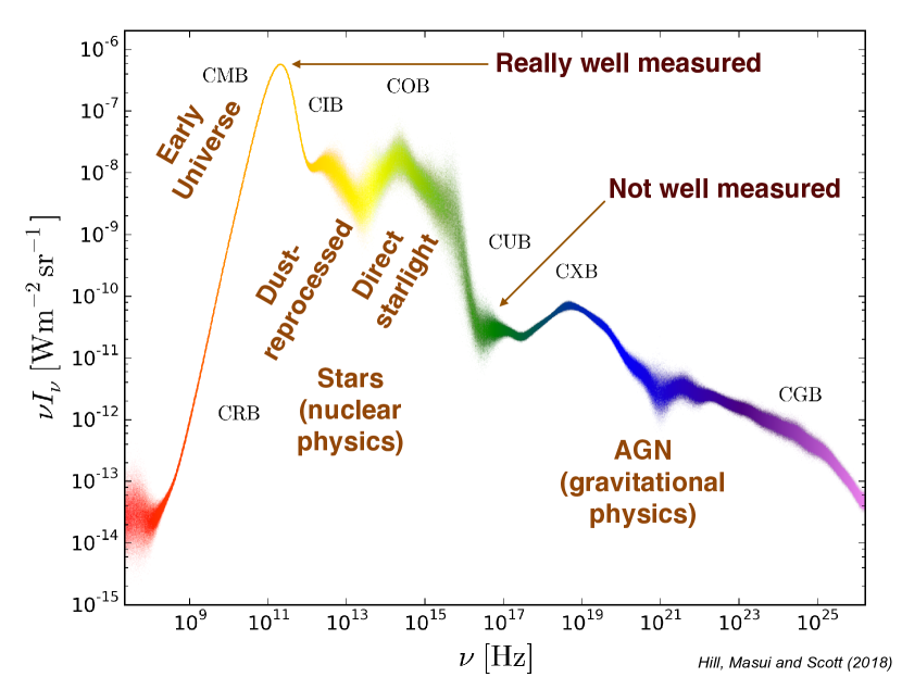
Figure 2: Recent summary of constraints on the extragalactic photon background, the “spectrum of the Universe”, with the width of the line indicating how uncertain the measurements are. The vertical axis here is intensity times frequency, which gives the contribution per logarithmic interval to the total intensity, and is also proportional to the energy density.

4 $\nu$ background spectrum

The CNB is similar to the CMB. One important difference is that neutrinos obey Fermi-Dirac instead of Bose-Einstein statistics. That means that although the spectrum is thermal, the distribution function in the spectrum has the form $\{\exp(E/kT)+1\}^{-1}$ rather than $\{\exp(E/kT)-1\}^{-1}$. Another difference is that the neutrino temperature is $1.9454\,$K, rather than the $2.7255\,$K of the CMB [28]. This comes from the fact that as the Universe expanded and cooled, the cosmic neutrinos decoupled before the last particle annihilation, namely that of electrons and positrons. As the temperature dropped below the electron rest mass, the CMB was boosted by the extra annihilation photons. By comparing entropy densities before and after this annihilation process, the ratio of neutrino to photon temperatures can be shown to be $(4/11)^{1/3}$ [29].

Another important difference between the CNB and CMB is that because neutrinos have mass, they are no longer completely relativistic. The results of neutrino oscillation experiments tell us that at least two of the neutrino flavours will be non-relativistic by the present time. So how does this affect the spectrum?

For photons in an expanding universe, the temperature scales with redshift as $T(z)=T_{0}(1+z)$ and the frequency as $\nu(z)=\nu_{0}(1+z)$, so that the factor $\{\exp(h\nu/kT)-1\}^{-1}$ retains its shape at all redshifts. This is true whether you consider the frequency or the energy or the momentum to be the quantity that redshifts (because for photons, all these quantities are the same, up to physical constants). However, for neutrinos, it turns out that it’s really the momentum that redshifts and so $\{\exp(pc/kT)+1\}^{-1}$ keeps its shape [30].

What this implies is that if we plot the CNB as a function of momentum, then all three neutrino flavours will have the same shape, but if we plot as a function of energy, then things are more complicated. Since $E^{2}=p^{2}c^{2}+m^{2}c^{4}$, then for massive enough neutrinos, the energy will be dominated by the neutrino’s rest mass. This is indicated in Fig. 3 for the minimal model consistent with neutrino oscillation results: $m_{1}\simeq 0$; $m_{2}\simeq 9\,$meV; and $m_{3}\simeq 50\,$meV. There are three separate CNB curves on the figure, with the two massive neutrino states being essentially spikes, where the energies pile up at the rest masses [31].

Figure 3 gives a broader representation of the neutrino version of Fig. 2 [32]. It’s plotted in units of energy density per unit energy times energy (like for the photon background, approximately showing contributions to energy density). As well as the CNB, there are other extragalactic neutrino sources. There will be neutrino spectral features coming from big-bang nucleosynthesis, in the same way that the CMB spectrum will contain weak line features from atomic recombination (e.g. Ref. [33]). The Sun is a locally dominant source of neutrinos, giving both thermal and nuclear emission features – stars in our Galaxy will contribute neutrinos at essentially the same energies (roughly MeV), but with perhaps $10^{8}$ times lower flux, while extragalactic stellar neutrinos will give a density another couple of orders of magnitude weaker [34]. These neutrinos will be an average over the spectra from all types of star, with the widths of nuclear neutrino lines being broadened by the redshift spread of distant galaxies. The extragalactic neutrinos will therefore give a spectrum like the Solar one, but about $10^{10}$ times lower in amplitude, redshifted in energy by about a factor of 2 and smeared by the width of $\Delta z\sim 1$ for star-forming galaxies. If we could detect them they would give a direct measure of the history of star formation, with no correction needed for interstellar extinction (like the case for photons).

There are also neutrino backgrounds expected from distant supernovae (sometimes called the “diffuse supernova background”), from AGN (perhaps already partly being detected by IceCube) and from cosmic rays (also called “cosmogenic” neutrinos). The positions of each of these background sources are represented approximately in Fig. 3 – so this figure is really a cartoon compared with the analogous photon-background plot.

Figure 3: Extragalactic neutrino backgrounds. The dotted line is the CMB, represented as energy density per unit energy, multiplied by energy. In a similar way, the solid curves show the CNB (for a minimal set of neutrino masses). The other labels indicate the approximate locations in this plane of several other contributions to the extragalactic neutrino background. Apart from perhaps at the highest energy end, this plot is essentially devoid of direct data constraints.

5 $\nu$ mixing

A fundamental difference between neutrinos and photons is that there are three flavours of neutrino, but a photon is just a photon. However, it’s even more complicated than this because the flavour states can mix into each other [35]. Mass states aren’t flavour states and the mixing matrix is far from being diagonal. In other words, it’s hard to answer a question like “what’s the mass of the electron neutrino?”

Neutrinos interact in flavour states, but propagate in mass states and if CNB detectors existed, they would presumably be sensitive to particular flavour states. That means that the neutrinos in the CNB decouple in the early Universe as $\nu_{e}$, $\nu_{\mu}$ and $\nu_{\tau}$, but propagate to us as $\nu_{1}$, $\nu_{2}$ and $\nu_{3}$. If we could easily detect them, then we’d have to consider whether we were detecting, say, just $\nu_{e}$s or all flavours, and we’d have to take the mixing into account. For example, with what we know about the mixing matrix, an experiment that detects electron neutrinos from the CNB will be detecting approximately 68 % of the smallest mass state ($m_{1}\simeq 0$), 30 % of the next mass state ($m_{2}\simeq 9\,$eV in the normal hierarchy) and only 2 % of the most massive state ($m_{3}\simeq 50\,$meV).

6 $\nu$ speeds

The CNB neutrinos were in equilibrium with other particles until the weak interactions froze out at $t\sim 1$ s in the history of the Universe. At those early times the neutrinos had energies that were much higher than their rest masses and hence they were ultra-relativistic. Their momenta redshifted according to $p\propto(1+z)$, which means that the Lorentz factor $\gamma\propto(1+z)$ until $\gamma\simeq 1$ (so $v\simeq c$), after which $v\propto(1+z)$. The transition happened when momentum was approximately rest mass (times $c$).

In the simplest scenario, the two heavier mass-state neutrinos are now non-relativistic, while the lightest mass state is still relativistic. The average speed of cosmic neutrinos, after they become non-relativistic is

$$\left\langle v_{\nu}\right\rangle\simeq 150\,\left({{\rm eV}\over m_{\nu}}\right)\,{\rm km}\,{\rm s}^{-1}$$ (3)

(e.g. Ref. [36]). This means that for a 50-meV mass state (probably the heaviest in the normal hierarchy), the transition to the non-relativistic regime happened at $z\simeq 100$ and the average speed is now about $3000\,{\rm km}\,{\rm s}^{-1}$, i.e. only 1 % of the speed of light. If the second mass state is around 9 meV, then those neutrinos are travelling about 6 times faster than the heaviest neutrinos, while the lowest mass state is still relativistic today. If the hierarchy is inverted, then slower speeds could prevail.

7 $\nu$ last-scattering surface(s)

Cosmic neutrinos decoupled in the early Universe when the rate of weak interactions, like $p+e^{-}\leftrightarrow\nu_{e}+n$, became too slow compared with the expansion rate. This occurred when average particle energies were around 1 MeV, at $t\sim 1$ s and redshift $z\sim 10^{10}$. We can thus think of a “neutrino last-scattering surface” (LSS) in analogy with the CMB LSS, which happens at $t\simeq 380{,}000$, $z\simeq 1100$.

However, the last section described how some neutrinos have been non-relativistic for quite some time. As first pointed out by Bisnovatyi-Kogan & Seidov in 1983 [37] (and described more explicitly by Dodelson & Vesterinen [38]), the finite speed of neutrinos means that it is possible for the distance to the neutrino LSS to be significantly smaller than the distance of the photon LSS, even though the neutrinos decoupled from the rest of the matter much earlier than the photons did [39]. Neutrinos aren’t on the light cone, but instead they live on the neutrino cone (which makes an angle $<45^{\circ}$ with the time axis). As shown by Dodelson & Vesterinen, for neutrino masses greater than about 0.1 meV, the CNB LSS will be closer than the CMB LSS.

The situation is made more interesting because of the multiple flavours of neutrino and the mixing of those flavours. There will actually be three distinct LSSs, one for each mass state, since those have different average speeds. In more detail, the distance will be different for every neutrino momentum in the Fermi-Dirac distribution, and hence each LSS will be quite wide in distance. With a detector, say of $\nu_{e}$s, a fraction will come from each of the broad LSSs corresponding to the three mass states [40].

The fact that neutrinos live off the light cone gives the potential prospect of seeing the same cosmological structure at two different epochs, one using neutrinos (at an earlier time) and the other using photons (at a later time) [41]. We could imagine some overdense region where varying gravitational potential (“ISW”) or lensing effects might be detectable in both photons and neutrinos. Then one could directly measure the growth of the overdensity between the two epochs, yielding a new way to constrain the behaviour of the fluids affecting the growth, e.g. the equation of state of the dark energy [42].

8 $\nu$ anisotropies

The CMB contains anisotropies arising from density perturbations in the early Universe [43], and this will also be true for the CNB. The first publication of a prediction of the CNB anisotropy power spectrum was in a 1995 paper by Hu, Scott, Sugiyama & White [44]. The relevant plot [45] showed that there would be an enhancement in the $C_{\ell}$s at about the CMB LSS horizon size because of the “early ISW” effect, raising the power spectrum to a plateau that would continue out to the scale of the CNB LSS, with damping at multipoles $\ell\sim 10^{8}$ (i.e. milli-arcsecond angular scales).

This initial calculation ignored the “late ISW” effect that gives an extra contribution at low multipoles (as it does for the CMB), because of gravitational potentials changing fairly recently in the history of the Universe. Examples of more accurate calculations from some more recent theoretical studies are shown in Fig. 4. Mostly these have focussed on the low-$\ell$ regime [46, 47, 48]. At higher multipoles, the most detailed analysis is in the 2015 Ph.D. thesis of Elham Alipour, supervised by Kris Sigurdson at UBC [49]. The calculations are complicated to get right, and also computationally challenging. That’s because each momentum state in the neutrino distribution function has to be evolved separately – different momenta travel at different speeds after all! This means that when running a Boltzmann solver, in addition to following sets of $k$ (Fourier-space) modes and spherical harmonic (angular) modes, there also has to be a loop sampling over the momentum space (which is of course unnecessary for photons, all of which propagate at the speed of light).

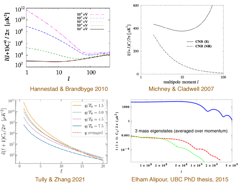
Figure 4: Some published calculations on CNB anisotropy (actually almost all of them).

If we could figure out a way to measure the CNB anisotropies, then they would in principle yield astonishingly precise cosmological constraints. The information content of a 2-d Gaussian field, like the CMB sky, is just a matter of mode counting, with the number of modes out to a maximum multipole $\ell_{\rm max}$ scaling as $\ell_{\rm max}^{2}$ [50]. The number of available modes in the CNB is thus a factor of around $10^{10}$ larger than for the CMB. The CNB power spectrum is fairly flat out to high $\ell$, lacking the deep oscillatory structure in the CMB power spectrum, so the CNB anisotropies would not necessarily improve all cosmological parameter constraints by such a large amount, but nevertheless, the resulting uncertainty on some parameters (e.g. the scalar spectral index, $n_{\rm s}$) would be extraordinary. And, as shown by Alipour, oscillatory structure in the damping tail (at $\ell\sim 10^{9}$) would likely yield further parameter constraints [51].

9 $\nu$ inhomogeneities

Treating CNB anisotropies in analogy with CMB anisotropies isn’t quite the right thing to do though. That would be fine if cosmic neutrinos were still completely relativistic, but they’re not. At the other (non-relativistic) extreme, we have CDM particles, which are “cold” today, meaning that their typical velocities are negligible for the purposes of structure formation. The CDM sky has no anisotropies that are remnants of the epoch when those particles decoupled in the early Universe, since the trajectories have been dramatically altered by interaction with gravitational potentials. Instead of primordial anisotropies on the sky, CDM particles exhibit spatial clustering, i.e. inhomogeneities, with enhancements in potentials and streams from halo interactions as structures merge together.

There have been quite a few studies of the clustering of cosmic neutrinos, either through analytical calculations or treating them as particles in simulations, [52, 53, 54, 55, 56, 57, 58]. These analyses look at how neutrinos might be enhanced in the halos of galaxies, or perhaps in the Solar neighbourhood of our own Galaxy. The consensus view is that effects of neutrino enhancement in galaxy halos are relatively weak, at perhaps the few percent level.

Cosmic neutrinos lie somewhere (in their behaviour) between photons and CDM particles. So, to fully treat their fluctuations we need to consider both the primordial anisotropies and also the changes caused by gravitational interactions while they (or at least some of them) were non-relativistic.

These effects will include gravitational lensing. The usual calculation of the gravitational bending angle gives

$$\alpha={4GM\over c^{2}b},$$ (4)

for a photon passing mass $M$ at impact parameter $b$. Since this involves the square of the speed in the denominator, then for neutrinos moving at $v\ll c$, the deflections can be much larger than for photons [59]. It was pointed out earlier that the highest mass neutrinos have average speeds today that are about 100 times slower than $c$. Hence a deflection through a galaxy cluster that would bend photons by arcminutes could completely change the trajectory of a slow neutrino. Indeed, there will be situations where the path is bent so much that the neutrino is captured by the mass, which is when “lensing” turns into “clustering”.

Some strong lensing effects for CNB neutrinos were investigated by Yao-Yu Lin & Holder [60], showing for example that the chromatic nature of neutrino lensing means that it would be possible to probe the whole causal volume. These studies are separate from the related topic of investigating photon lensing in halos affected by neutrinos (e.g. Refs. [61, 62]). A full analysis of all anisotropy, clustering and lensing effects in the CNB has yet to be done.

10 $\nu$ dipoles

The largest scale anisotropy in the CNB will be the dipole. Just as is the case for the CMB, the dipole is expected to be dominated by our motion relative to the universal “rest frame” (e.g. Ref. [63]). The dipole can also been measured in the anisotropy of the distribution of sources on the sky, such as galaxies or AGN. If these sources are close enough then there will also be a dipole component caused by source clustering. Inhomogeneities in the cosmic neutrinos could therefore affect the size and direction of the dipole. For the CNB, the dipole could (at least in principle) be measured for different flavours, coming from different combinations of mass states, and this could be done for different neutrino momenta, probing different volumes.

There have been papers suggesting related tests. For example, there is a possibility of using the range of low-order neutrino anisotropies as a function of momentum to perform a test of the Copernican principle [64]. And the annual modulation of the CNB could also potentially be used to extract the cosmic neutrino signal [65, 66, 67] – this is essentially using the time-variation of the dipole a bit like the “orbital dipole” is used to calibrate CMB measurements.

11 $\nu$ indirect detection

If the CNB is so hard to detect, why are we so confident that it exists? The most important reason is that there’s strong (if indirect) evidence of the CNB through the precision measurements of CMB anisotropies. The neutrinos contribute at early times to the relativistic background (or “radiation”), affecting the expansion rate to such an extent that the CMB data cannot be fit without including the neutrinos (which give 68 % extra energy density compared to the photons). Since matter-radiation equality happens not much earlier than the cosmic recombination epoch, then radiation is still important at the recombination time and in fact $\rho_{\nu}\sim 0.1\rho_{\rm tot}$ at the CMB LSS, making it clear why the CNB is far from negligible.

The strength of this effect can be assessed through the effective number of light degrees of freedom, $N_{\rm eff}$. For three neutrino flavours we would expect $N_{\rm eff}=3$, except that detailed calculations, including non-instantaneous decoupling, oscillation effects, finite-temperature effects, etc. [68], give $N_{\rm eff}=3.044$ [69] as the currently best accepted value (with theoretical uncertainties being in the last digit).

The Planck data, including CMB lensing, combined with baryon acoustic oscillation (BAO) measurements from galaxy surveys (see Ref. [8] for details and references) gives

$$N_{\rm eff}=2.99\pm 0.17.$$ (5)

This effectively corresponds to a $17\,\sigma$ detection of the CNB.

In addition, the neutrinos should have two parameters that describe the behaviour of their perturbations, $c_{\rm eff}$, the sound speed, and $c_{\rm vis}$, which parameterises the anisotropic stress. Both are expected to have the same value for non-interacting massless neutrinos, namely $c_{\rm eff}^{2}=c_{\rm vis}^{2}=c^{2}/3$. Treating these as additional free parameters and fitting to the Planck data yields values of $0.324\pm 0.006$ and $0.327\pm 0.037$, both consistent with expectations, and an anisotropic stress of zero is rejected at the $9\,\sigma$ level [70]. A related effect is a phase shift in the CMB power spectra, caused by the anisotropic stress, which has also be measured [71].

To summarise these results: the CNB has been detected, indirectly, through its effect on CMB anisotropies. We know that before the recombination epoch there were three species of relativistic particles, which had the same properties as expected for neutrinos. Because of the strength of this evidence, the standard $\Lambda$CDM model includes the CNB, with fixed properties.

The standard cosmological model (SMC [72, 73]) is $\Lambda$CDM, with a parameter space spanned by six parameters, e.g. $\Omega_{\rm b}h^{2}$, $\Omega_{\rm c}h^{2}$, $\theta_{\ast}$, $A_{\rm s}$, $n_{\rm s}$ and $\tau$. The temperature of the CMB would be a 7th parameter, but this is so well determined that it is usually considered to be fixed, rather than being allowed to float when fitting power spectra (but see Ref. [74]). The SMC isn’t like the standard model of particle physics, which has a clear mathematical basis and hence a fixed amount of freedom. Most cosmologists are expecting that eventually we’ll need more parameters to describe the SMC, hopefully with some genuine surprises. The next parameter that we think we’re about to require is related to neutrino mass.

12 $\nu$ mass

The sum of the neutrino masses is usually written $\sum m_{\nu}$. But an expression is an awkward notation to use for a parameter, and it would be better called something such as ${\cal M}_{\nu}$. The Planck Collaboration used a basic cosmological model that includes the CNB with a single mass eigenstate having $m_{\nu}=0.06\,$eV. But it would make no difference to the fit if the mass was split between two or three neutrinos – the sensitivity is essentially to ${\cal M}_{\nu}$ alone, and not how the mass is distributed among types of neutrino.

The tightest constraints from the CMB alone come when including CMB lensing, giving numbers like ${\cal M}_{\nu}<0.25\,$eV at 95 % confidence from the Planck 2018 data set [8]. Combining with BAO data yields even stronger constraints. Currently the tightest limit comes from using the newest analysis of the “Public Release 4” Planck data [9] in combination with BAO results, yielding

$${\cal M}_{\nu}<0.11\,{\rm eV}\ (95\,\%)\ \cite[cite]{[\@@bibref{}{2dplane}{}{}]}.$$ (6)

This is coming very close to ruling out the inverted mass hierarchy, which requires ${\cal M}_{\nu}\mathrel{\hbox to0.0pt{\lower 3.0pt\hbox{$\mathchar 536\relax$}\hss}\raise 2.0pt\hbox{$\mathchar 318\relax$}}0.1\,$eV (e.g. Ref. [76]).

Right now the evidence for the existence of the CNB does not require the neutrinos to have any mass. We need to include the CNB to fit the Planck satellite data, but a fully relativistic (i.e. massless) CNB is sufficient for now. However, that situation is expected to change soon, as cosmological data become increasingly precise.

There are three separate effects of neutrino mass on the CMB, all of which contribute to current constraints on ${\cal M}_{\nu}$:

1. changing the distance to the CMB LSS;

2. smoothing of power spectra at small scales;

3. changing the shape of the lensing power spectrum.

This last item is particularly important, especially as ground-based CMB experiments push to higher sensitivity and angular resolution, and is expected to be the cleanest way of detecting neutrino mass. Additionally, massive neutrinos change the shape and growth history of the matter power spectrum (relative to the CMB amplitude), although the effect occurs on small scales, where the power spectrum becomes nonlinear.

Tight constraints are expected to come from combining the CMB with surveys that measure the expansion rate at low redshifts, e.g. from the BAO scale. The Euclid satellite is expected to achieve a $1\,\sigma$ uncertainty on ${\cal M}_{\nu}$ of around 30 meV [77]. The Dark Energy Spectroscopic Survey Instrument [78] and Rubin/LSST are similar [79]. Future CMB experiments such as CMB-S4 will also provide important constraints through the effect on CMB lensing; better determination of the reionisation optical depth, such as provided by the LiteBIRD satellite [80], will help break parameter degeneracies to enable improved ${\cal M}_{\nu}$ determination. Overall there is an expectation that an uncertainty of around 20 meV is possible (e.g. [81, 82, 83]), perhaps even as small as 10 meV if all constraints are combined.

13 $\nu$ exotica

Theorists are creative, and hence there are many ideas for extending the physics of neutrinos to make things more complex. One commonly discussed addition to the neutrino family is to consider an extra type that has essentially no interactions, and hence is called a “sterile” neutrino [84]. This could have a different distribution function than the normal CNB types and hence contribute as a fraction (rather than an integer) to the value of $N_{\rm eff}$. An extra (fourth) kind of neutrino would involve additional mixing matrix parameters, such as $\sin^{2}2\theta_{14}$, and squared mass-splittings, such as $\Delta m_{41}^{2}$. The two-dimensional space of $(\sin^{2}2\theta_{14},\Delta m_{41}^{2})$ can be related to the cosmological parameters $({\cal M}_{\nu},N_{\rm eff})$. However, one needs to be careful with volume effects, sampling and priors, in order to properly transform between the particle-physics and cosmological parameter spaces [85, 86].

There are plenty of other ideas that could change the physics of the CNB. Perhaps the least speculative is the possibility that there might be a non-zero chemical potential in the neutrinos, or other changes to the Fermi-Dirac spectrum. They could exhibit decays, annihilations, self-interactions, other non-standard interactions, Lorentz violation or additional kinds of oscillation. There could also be new sources of low-energy neutrinos that complicate the interpretation of the CNB. Much more could be said about these and other possibilities, but we shall stop here.

14 $\nu$ conclusions

The CNB undoubtedly exists, with clear evidence of its early-time effects on the CMB, when still part of the relativistic background. The inferred count of relativistic species is consistent with the number three [87], and the behaviour of the fluid perturbations is also in line with what we expect for the CNB.

Current cosmological data place a limit on the sum of the neutrino masses, ${\cal M}_{\nu}$, which is only a factor of 2 or so from the minimum expectation from neutrino oscillation experimental results. The inverted hierarchy is already close to being ruled out (or confirmed for that matter) by the data. Cosmologists are now excited about the possibility of actually constraining ${\cal M}_{\nu}$ to be non-zero through the effects of neutrino mass on the power spectra of CMB anisotropies (particularly lensing) and galaxy clustering. Combining all the measurements expected in about the next decade should enable a measurement of ${\cal M}_{\nu}$ at around the $5\,\sigma$ level, even for the minimal mass limit in the normal hierarchy.

However, there’s an elephant in the room (Fig. 5). There are many particle experimentalists working hard to try to detect the neutrino mass directly and the question is – will they take seriously a cosmological detection of ${\cal M}_{\nu}$? It seems that the chasm between the two sub-fields has been closing, and nowadays both particle and astro researchers tend to appreciate the complementarity of the approaches. The cosmological measurement of neutrino mass might be indirect and “model-dependent”, but the model is understood to be really a very simple one that already fits the data astonishingly well. There are multiple kinds of cosmological observable that can be affected by massive neutrinos, and if two or more start to point towards some value of the total neutrino mass, then that will have to be taken very seriously. Of course it will still be useful to make more direct measurements of neutrino mass, as well as to determine what each of the individual masses are. And on the flip side, although future particle-physics experiments might be able to reach down to the neutrino mass scale, they are very very far from being able to detect the neutrinos in the CNB itself.

Perhaps through the pursuit of increasingly sensitive ways of probing low-energy neutrinos, we might eventually reach a situation where the CNB can be observed directly, enabling us to probe cosmological perturbations at the neutrino decoupling epoch. It’s not going to happen soon, but we can dream!

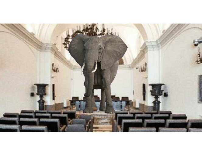
Figure 5: The elephant in the room. In this case, the Fermi Room, where the lectures of this summer school were given.