[orcid=0000-0003-0494-5098] \creditConceptualization, Methodology, Software, Investigation, Writing – original draft \creditData curation, Validation, Formal analysis, Writing – review & editing \creditConceptualization, Writing – review & editing \creditResources, Writing – review & editing \creditData curation, Resources, Writing – review & editing \creditConceptualization, Writing – review & editing \creditConceptualization, Writing – review & editing, Supervision \cormark[1] \creditConceptualization, Writing – review & editing, Project administration, Supervision, Resources, Funding acquisition
1]organization=Institute of Health Informatics, University College London, city=London, postcode=NW1 2DA, country=UK 2]organization=Department of Psychiatry, University of Oxford, city=Oxford, postcode=OX3 7JX, country=UK 3]organization=Department of Diabetes & Endocrinology, University College London Hospitals,city=London, postcode=NW1 2PG, country=UK 4]organization=Centre for Obesity & Metabolism, Dept of Experimental & Translational Medicine, University College London,city=London, postcode=WC1E 6JF, country=UK 5]organization=Centre for Bio-Inspired Technology, Department of Electrical and Electronic Engineering, Imperial College London,city=London, postcode=SW7 2AZ, country=UK
6]organization=FLock.io,city=London, postcode=WC2H 9JQ, country=UK 7]organization=Department of Computer Science, University College London,city=London, postcode=WC1E 6EA, country=UK
[1]Corresponding author
GARNN: An Interpretable Graph Attentive Recurrent Neural Network for Predicting Blood Glucose Levels via Multivariate Time Series
Abstract
Accurate prediction of future blood glucose (BG) levels can effectively improve BG management for people living with diabetes, thereby reducing complications and improving quality of life. The state of the art of BG prediction has been achieved by leveraging advanced deep learning methods to model multi-modal data, i.e., sensor data and self-reported event data, organised as multi-variate time series (MTS). However, these methods are mostly regarded as “black boxes” and not entirely trusted by clinicians and patients. In this paper, we propose interpretable graph attentive recurrent neural networks (GARNNs) to model MTS, explaining variable contributions via summarizing variable importance and generating feature maps by graph attention mechanisms instead of post-hoc analysis. We evaluate GARNNs on four dataset, representing diverse clinical scenarios. Upon comparison with twelve well-established baseline methods, GARNNs not only achieve the best prediction accuracy but also provide high-quality temporal interpretability, in particular for postprandial glucose levels as a result of corresponding meal intake and insulin injection. These findings underline the potential of GARNN as a robust tool for improving diabetes care, bridging the gap between deep learning technology and real-world healthcare solutions.
keywords:
Blood glucose prediction \sepInterpretable \sepGraph \sepRecurrent neural networks \sepDiabetesWe propose GARNNs to forecast blood glucose levels, providing prediction explanations by learning temporal variable importance.
GARNNs are based on graph attention to assess and prioritize temporal variables for the forecasting.
GARNNs offer insightful feature maps for the prediction, supported by theoretical proofs.
GARNNs are rigorously tested against twelve baselines, proving superior accuracy and interpretability for the prediction.
GARNNs’ effectiveness across four datasets is demonstrated by their robustness for sparse input signals, such as insulin and meal intake.
1 Introduction
Diabetes is directly responsible for over a million deaths worldwide every year [1] due to complications arising from type 1 diabetes mellitus (T1DM) and type 2 diabetes mellitus (T2DM). The autoimmune reaction of people with T1DM destroys the cells in the pancreas which produce endogenous insulin, while people with T2DM predominantly have insulin resistance, which inhibits their ability to utilize insulin effectively. Difficulties to manage BG levels by endogenous insulin leads to hypoglycemia and hyperglycemia, causing serious health problems [2, 3]. Hence, effective self-management for BG levels is the key to the treatment [4], because increased “Time in Range” has been shown to reduce the likelihood of complications [5].
Continuous glucose monitoring (CGM) systems offer the ability to track BG levels every few minutes, generating continuous BG trajectories. BG level prediction (BGLP) based on CGM data [6, 7] allows people with diabetes to avoid hypo- and hyperglycemia by taking precautions in real-time. Recent work [8, 9, 10, 11, 12] leverages multi-modal data by organizing it as MTS in BGLP. In this case, apart from CGM data, the MTS input also includes sensor data, e.g., heart rate, and self-reported events, e.g., the amount of carbohydrate intake and bolus insulin injection. While these methods have the potential to further improve BGLP by levaraging the rich hidden information of MTS, the lack of interpretability makes them less trustworthy. It is vital to understand how each variable contributes towards prediction rather than solely improving prediction accuracy.
However, post-hoc analysis methods, e.g., gradient-based attribution methods [13], are computationally inefficient [14] and difficult to be used by the researchers and clinicians without machine learning knowledge. Shapley Additive exPlanations (SHAP) values, as discussed by Lundberg and Lee in [15], are utilized alongside Long Short-Term Memory (LSTM, [16]) models in BGLP [17, 18]. It should be noted that while they offer significant insights into the importance of a limited number of variables, their scope in temporal variable importance is somewhat restricted.
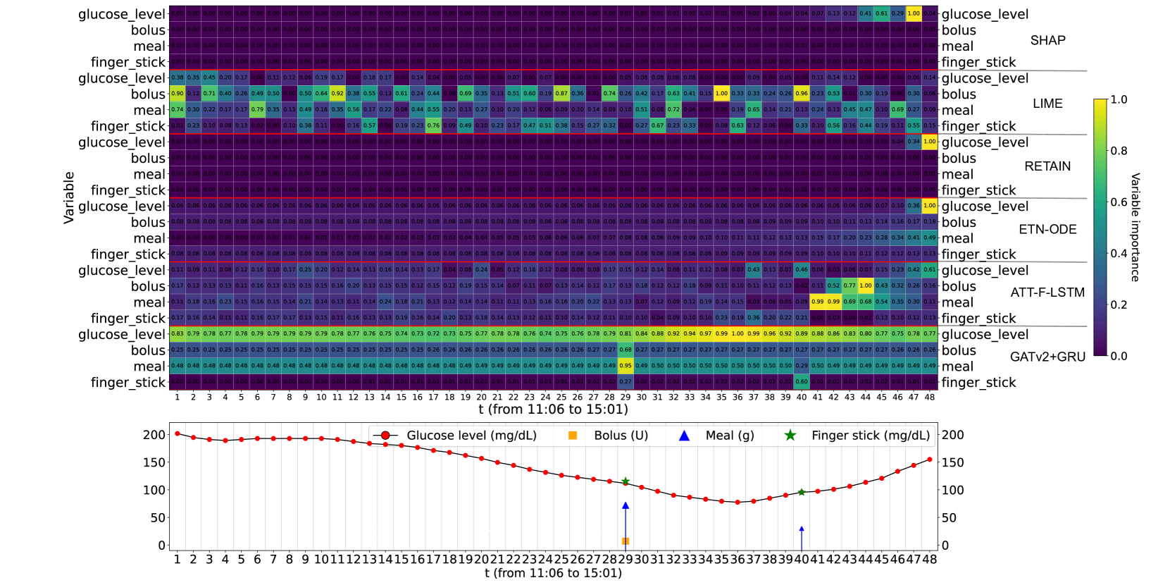
Comparably, attention-based recurrent neural networks (RNNs), e.g., RETAIN [20], ETN-ODE [21] and ATT-F-LSTM [22], can inherently learn variable importance by the attention mechanisms during training. Nevertheless, the feature maps built on the variable importance are unhelpful to understand BGLP. Hence, we aim to propose a novel attention-based interpretable model that can rank variables in accordance with domain knowledge and generate understandable feature maps. For instance, figure 1 demonstrates the comparison of existing interpretable methods in interpreting the time-dependent importance of self-reported events for BG trajectories. Other interpretable methods fail to present their correct focus on self-reported events, as shown in their feature maps. On the contrary, our proposed method “GATv2+GRU” provides insights into the importance of variables when valid observations are available for those variables. For instance, in our feature map, the importance of “bolus” suddenly increases from to at , because this participant administrated bolus insulin at this timestep. When data is incomplete or invalid, like when missing points are filled with average values, the importance of variables tends to become stable at certain numbers. In such cases (), the importance of “bolus” typically remains near , reflecting an average importance due to this data padding. Besides, it can precisely capture the local maxima and minima. When , the “glucose_level” achieves its lowest local minima, and its importance increases to .
When compared with both non-interpretable and interpretable approaches, our proposed methods outperform others in BGLP. Additionally, they offer effective explanations for MTS by inherently providing detailed insights. To summarize, the contributions of this paper are as follows:
-
•
We propose Graph Attentive Recurrent Neural Networks, denoted as GARNNs, combining Graph Attention neTworks (GAT [25] or GATv2 [23]), with RNNs. We leverage GAT/GATv2 to explicitly model correlations among various variables, resulting in the inherent learning of temporal variable importance. Subsequently, RNNs are employed to aggregate temporal features for the prediction of future BG levels.
-
•
We propose a novel temporal variable importance for MTS based on graph attention mechanisms. It can respectively summarize and generate significant variable importance ranking and feature maps in BGLP. We employ three theorems and their corresponding proofs to demonstrate the creation, characteristics, and influence of temporal variable importance.
-
•
Our methods, along with twelve baseline approaches, are assessed using four datasets. This evaluation focuses on the accuracy of predictions and the significance of variable ranking and feature maps. Not only do our methods exhibit outstanding performance, but they also attribute medically justifiable significance to crucial variables, including those with sparse signals like insulin injections and meal intake.
2 Related Work
Interpretable methods can be generally divided into post-hoc analysis methods and attention-based methods.
If a model itself lacks interpretability, it is still possible to derive explanations via post-hoc analysis methods, e.g., gradient-based analyzing [26, 27], variable contribution to the temporal shift of model [28], Local Interpretable Model-agnostic Explanations (LIME, [19]). SHapley Additive exPlanations (SHAP, [15]), shapley based feature attributions [29] and local rule based explanation [30].
However, considering the efficiency and the target to explain the modeling of each MTS, the above methods are not considered in BGLP. Instead, we focus on attention-based methods, where variable importance based on attention is inherently learned during training.
Tensorized RNN methods [14, 31, 32, 33, 21] leveraged parallel RNNs to model MTS, where each time series was modeled by a certain RNN. Then, they used attention to aggregate the outputs of parallel RNNs. In this regard, IMV-TENSOR [14] leveraged variable-wised temporal attention and variable attention to summarize all the outputs of parallel LSTMs, where the attention was directly mapped from the outputs of LSTMs by fully-connected layers. Similarly, instead of using parallel RNNs, Hsieh et al. utilized parallel 1-dimensional convolution neural networks for modeling MTS aided by attention [34].
These parallel structures explicitly split the contribution of variables in the prediction, but they ignored the interaction among the variables. Besides, extracting variable importance from the temporal attention which worked on the outputs of RNNs could cause temporal biases. For example, as shown in Figure 1, we cannot infer the variable importance of “meal” from the feature map of ETN-ODE, when . This is because some important content at is passed to the last several timesteps by RNNs, and feature maps are built on the outputs of RNNs. While RETAIN [20] and RAIM [35] did not incorporate parallel structures and utilized the attention mechanism to combine embeddings of MTS instead of RNN outputs, their attention process was still influenced by the outputs from RNNs. For instance, RETAIN employed two separate RNNs to create attention at both the visit and variable levels. This RNN-derived attention was then applied to aggregate the MTS embeddings. Consequently, in RETAIN, the significance assigned to variables was somewhat biased by the RNNs, as illustrated in Figure 1.
Even though certain researchers had attempted to minimize the influence of RNNs on the importance of temporal variables, the effectiveness of this importance remained uncertain. Kaji et al. and Gandin et al. had implemented attention mechanisms prior to the RNN layers, ensuring that the variable importance was not skewed by the RNNs. However, this approach, which was directed either by variable-wise temporal attention [36] or time-wise variable attention [22], still led their models to erroneously focus on some irrelevant data points, particularly in the context of sparse signals. This issue is evident in models like ATT-F-LSTM [22], as showcased in Figure 1.
3 Preliminaries
Given a directed graph , we assume that the graph has nodes, denoted as . Each node is connected with its neighborhood , through the edges of . Besides, the presentations of all the nodes are , where the presentation of the node is . Assuming that there are multiple layers in Graph Attention neTworks (GATs), defined as , each node in layer can receive and aggregate neural messages from . Then, one of the aggregation approaches is:
| (1) | ||||
| (2) |
where the neural message from node is ; learnable parameters are and ; the attention weight from to is .
We temporarily omit the superscript for simplicity. The attention weight is gotten by normalizing the score . The score from node to node is , as:
| (3) | ||||
| (4) |
where and are learnable parameters; constant is a hyperparameter; the concatenation of vectors is .
The above score function can be rewritten as:
| (5) | ||||
| (6) |
where . The query is , and the key is . As for Equation (5), the learnable parameters should be the same as .
Based on the findings presented in [23], the scoring mechanism in GAT and GATv2 differs, with GAT having a static approach and GATv2 featuring a dynamic one. As a result, GATv2 demonstrates greater expressiveness in modeling intricate features of graphs, offering enhanced capabilities compared to its predecessor.
Static scoring: given queries and keys , it holds , where , , , .
Dynamic scoring: given queries and keys , it holds , where , , and . Meanwhile, function and .
4 Proposed model
4.1 Problem definition
Blood glucose level prediction based on multivariate time series (BGLP-MTS): given the values of variables from historical timesteps , i.e., , predict the BG level . The vector , and is a prediction horizon. We let be the target variable, i.e., . The rest variables () are exogenous variables when .
4.2 Overview
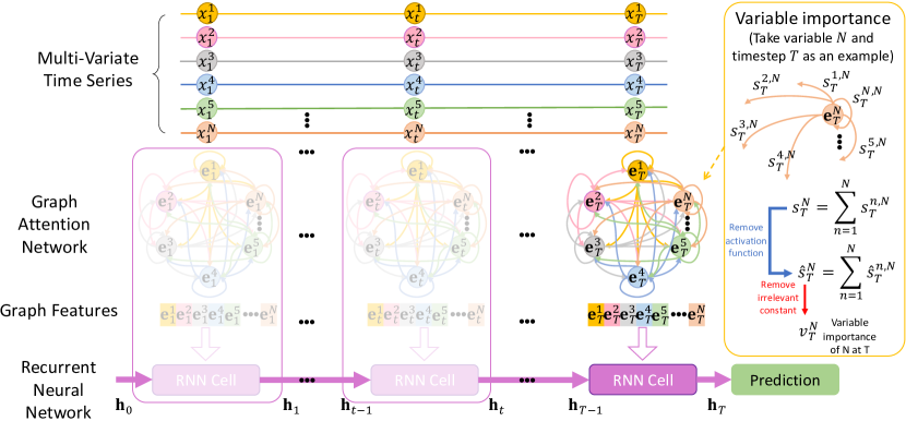
Our proposed models, GARNNs, build a graph at each timestep and use each node of the graph to represent a variable of MTS, assuming each graph is initially a complete graph (see Figure 2). Then, the input of Equation (1) is
| (7) |
where learnable parameters . Then, we can use Equation (1-2) aided by Equation (5) or Equation (6) to update representations of . Next, we collect the latest representations and concatenate them as .
After explicitly modeling correlations of these variables, we collect of all timesteps, denoted as . Then, we leverage RNN to aggregate them, as:
| (8) |
where we utilize gated recurrent unit (GRU, [24]) as to aggregate temporal features in this paper. Finally, the prediction is , where consists of fully connected neural networks.
Given training examples , the objective function is:
| (9) |
where are all the learnable parameters of our proposed model; is a hyperparameter.
4.3 Interpretability
Theorem 1.
There exists a universal interpretable variable importance of GAT and GATv2 .
Proof.
In BGLP scenario, we assume each node connects with all of the nodes of . Then, as for the neighbour nodes of the node , we have . Considering Equation (1-2) and Equation (5-6), for the variable , the higher the score , the more important to . The mean of the scores from to all variables of is denoted as:
| (10) |
It is the impact of the variable on all the variables. Theoretically, a higher level of importance assigned to variable corresponds to an increased mean score . As a result, an enhanced amount of information from is conveyed to and preserved within the embedding collected from GAT/GATv2, thereby amplifying the contribution of in the prediction process.
However, we do not regard as the variable importance of at timestep . Instead, we extract its variable importance from by removing irrelevant information. Specifically, considering that is monotonic with respect to , we remove from Equation (10). GAT and GATv2 can be organised in the same format, as:
| (11) | ||||
| (12) |
where is unequal and equal to in GAT and GATv2 repectively. Then, we define the variable importance by removing the irrelevant item from :
| (13) |
On the other hand, we can consider multiple layers of GAT or GATv2, the variable importance is defined as:
| (14) |
Given , the variable importance of over is:
| (15) |
where is the variable importance of at timestep of the -th sample; the total number of training examples is ; the length of the MTS is . ∎
As in Equation (13), our proposed variable importance is fully understandable. It consists of a variable contribution , a variable embedding and a constant bias . The variable contribution and constant bias are learnable, so is directly guided by the variable embedding . When , the variable importance is only affected by . When , the variable importance considers correlations of and other variables.
Theorem 2.
The variable importance is from static scoring.
Proof.
Considering that , when and is fixed, can be seen as a constant. is largely affected by . There can exist a , making . This observation holds for any if is fixed. The variable importance is extracted from which is the mean of over , so is from static scoring. ∎
The use of static scoring for determining variable importance aligns with our expectations, primarily because dynamic scoring does not guarantee consistent significance of variables. For instance, in the case of GATv2, if we arrange variable based on the value of among , the dynamic scoring leads to considerable fluctuations in the ranking of within as varies. Consequently, using from GATv2 as a measure of variable importance becomes unreliable.
In contrast, the ranking of in based on the value of in remains constant despite changes in . Averaging over to reevaluate the ranking of does not alter its position, emphasizing the necessity for static scoring in assessing variable importance. Furthermore, eliminating from also maintains the ranking of , supporting this approach.
Additionally, the implementation of variable importance based on static scoring does not interfere with the dynamic scoring function of GATv2 in mapping out variable correlations. This ensures that GATv2 remains both effective in modeling and consistent in calculating variable importance.
Theorem 3.
The difference between and is bounded by small values depending on the slope of .
Proof.
In terms of GATv2 (see Equation (6)), we have:
| (16) |
where is an indicate diagonal matrix, as:
and is the -th value of the vector .
| (17) | ||||
| (18) |
where vetorial angle is . The boundary of the difference between and is:
| (19) |
Equation (9) has a soft constraint for . Based on the theory of Lagrange multipliers, there exists a value that is equivalent to the hard constraint for , where is a small positive value. Then, for a learnable parameter , we can have . We assume each value of the input vector of each GATv2 layer belongs to . Given that and , we have:
| (20) |
Similarly, in terms of GAT, we have:
| (21) |
∎
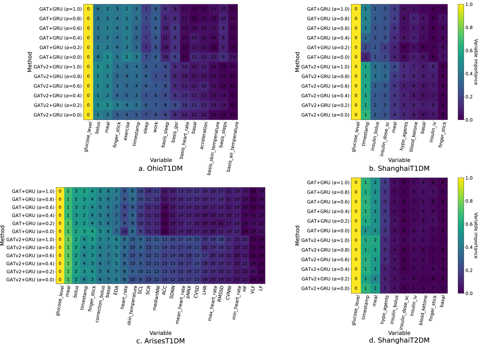
The bounds can be treated as the gaps between the modeling for prediction and the calculation of variable importance. The gaps are affected by . Nevertheless, changing has a slight impact on variable importance (see Figure 4). Hence, we hold the view that the small gaps between the prediction and the variable importance can be ignored.
5 Experiments
5.1 Datasets
We select four datasets containing multi-modal data with high quality, where T1DM and T2DM groups in Shanghai dataset [37] are regarded as two datasets. All datasets used in the study, except for ArisesT1DM (NCT ID: NCT03643692), are publicly accessible. The ArisesT1DM dataset was gathered in full compliance with relevant legal regulations. Consequently, ethical approval is not further required for this research.
OhioT1DM [38]: it is a well-validated dataset and has been used as a benchmark dataset in BGLP Challenges. It has 12 participants (age: 20-60 years; male/female: 7/5), containing 8 weeks’ CGM (Medtronic Enlite), sensor band (Empatica or Basis Peak) and self-reported data (meal, bolus, sleep, exercise, etc.). Each participant has more than 10,000 CGM measurements, and BG readings are sampled every 5 minutes ().
ShanghaiT1DM and ShanghaiT2DM [37]: it is a public dataset, consisting of 12 participants (age: 37-73 years; male/female: 7/5) with T1DM and 100 participants (age: 22-97 years, male/female: 44/56) with T2DM. It has 3-14 days’ CGM (FreeStyle Libre H) and self-reported data. There are 15,695 and 112,475 CGM measurements of people with T1DM and T2DM respectively, and BG readings are sampled per 15 minutes ().
ArisesT1DM (NCT ID: NCT03643692): it has 12 participants (age: 30–49 years; male/female: 6/6) and 6 weeks’ CGM (Dexcom G6), sensor band (Empatica E4) and self-reported data. Each participant has more than 10,000 CGM readings, and BG readings are sampled every 5 minutes (). In order to simplify the exhibition of experiment results, we leverage abbreviations of variable names [11], e.g., electrodermal activity (EDA).
OhioT1DM has been originally divided into training data and testing data by time for each participant. We further split the training data into the training part (80%) and validation part (20%). In terms of the rest three datasets, we respectively split the data into training data (60%), validation data (20%) and testing data (20%) by time for each participant. We use sliding windows to generate examples , i.e., and for , or and for . All the examples are normalized by standard normalization and padded by zeros. We consider almost all the variables (see Figure 3) in each dataset. However, certain variables with poor data quality, such as “stressors" in the OhioT1DM dataset, were excluded from our analysis.
5.2 Baselines
SHapley Additive exPlanations (SHAP, [15]) and Local Interpretable Model-agnostic Explanations (LIME, [19]): they are model-agnostic methods, providing variable importance for any methods. Given that our proposed methods got the best predicting performance compared with all of baseline methods, we leverage SHAP and LIME to explain our proposed methods for comparisons. We directly treat the absolute value of the variable importance provided by SHAP/LIME as , and is gotten by Equation (15).
Linear Regression (LR): it is a linear method. We flatten the input and use scikit-learn [39] to fit models. We aggregate the coefficients of the model as .
eXtreme Gradient Boosting (XGBoost, [40]): it is an optimized distributed gradient boosting approach. We flatten the input to fit models. We regard the average gain as , where the gain is collected across all splits when using variables.
REverse Time AttentIoN (RETAIN, [20]): it is an interpretable RNN model. The variable importance is calculated by the outputs of two RNNs, some learnable parameters and the input value of a variable. We use the absolute value of the variable importance of RETAIN as , and is gotten by Equation (15).
Interpretable Multi-Variable Long Short-Term Memories (IMV-LSTMs, [14]): both IMV-TENSOR and IMV-FULL are interpretable LSTMs by generating variable importance and variable-wise temporal importance. We directly average the variable importance of IMV-LSTMs with examples and regard the mean variable importance as . Meanwhile, we treat the variable-wise temporal importance as .
Explainable Tensorized Neural Ordinary Differential Equations (ETN-ODE, [21]): it consists of: 1) Tensorized GRU; 2) tandem attention; 3) ordinary differential equation network. Part 1 and 2 are for the interpretation, which is similar as IMV-TENSOR, and part 3 is for the arbitrary-step prediction.
ATTention of Time series before Long Short-Term Memory (ATT-T-LSTM, [36]): it separately adds temporal attention for each variable before passing through LSTM. We regard the temporal attention as , while cannot be calculated by this method.
ATTention of Features before Long Short-Term Memory (ATT-F-LSTM, [22]): it adds variable attention at each timestep before LSTM. Hence, the attention weight of a variable at timestep is , and is calculated via Equation (15).
Neural Basis Expansion Analysis for Interpretable Time Series forecasting (N-BEATS, [41]): it is a non-interpretable deep learning model for univariate time series modeling. It utilizes a stack of fully connected neural network layers to model time series data, offering remarkable accuracy and flexibility.
Neural Hierarchical Interpolation for Time Series forecasting (NHiTS, [42]): it is a non-interpretable deep learning model for MTS modeling, extending the N-BEATS and performing better in long-horizon prediction.
Our proposed method Graph Attentive Recurrent Neural Net- works (GARNNs) are represented by Graph Attention neTworks (GAT [25]) or GATv2 [23]) and Gated Recurrent Unit (GRU, [24]), i.e., “GAT+GRU” and “GATv2+GRU”.
All the deep methods are implemented by PyTorch 1.11.0 following their original codes on github and run with NVIDIA RTX 3090 Ti. All the methods except LR are trained four times by changing the random seed. In terms of XGBoost, we search for the learning rate in , n_estimators in , max_depth in , gamma in and min_child_weight in . For all the deep methods, we search for the learning rate in . For IMV-LSTM and ETN-ODE, we find the variable-wise hidden state size in . In terms of the rest deep methods, we search for hidden state size in . Besides, we also find in . We choose hyperparameters by the performance of the validation data based on the metrics in the following subsection.
5.3 Metrics
Considering the root mean square error (RMSE), mean absolute percentage error (MAPE) and mean absolute error (MAE), we also leverage the glucose-specific RMSE, denoted as gRMSE [43, 11], to evaluate all the methods. The gRMSE penalizes overestimation in hypoglycemia and underestimation in hyperglycemia. These two conditions can cause severe consequences to patients’ health. Besides, time lag is determined by analyzing the correlation between the forecasted BG levels and the actual readings from CGM.
5.4 Comparison of prediction performance
| Methods | RMSE (mg/dL) | MAPE (%) | MAE (mg/dL) | gRMSE (mg/dL) | Time lag (min) |
| LR | 22.190.00(2.79) | 10.900.00(2.13) | 15.920.00(1.95) | 27.690.00(3.72) | 8.340.00(6.06) |
| XGBoost | 22.510.04(3.32) | 10.920.04(2.24) | 16.080.05(2.26) | 28.890.08(4.77) | 9.360.12(6.47) |
| RETAIN | 20.300.08(2.64) | 9.780.04(1.81) | 14.410.03(1.75) | 25.480.16(3.47) | 7.390.09(4.95) |
| IMV-FULL | 21.610.32(2.99) | 10.210.18(1.79) | 15.180.23(1.89) | 27.160.40(4.16) | 6.420.28(4.50) |
| IMV-TENSOR | 20.150.03(2.77) | 9.540.02(1.82) | 14.000.02(1.75) | 25.420.07(3.79) | 7.570.11(4.86) |
| ETN-ODE | 21.000.22(2.92) | 10.110.13(1.95) | 14.780.18(1.93) | 26.410.32(3.94) | 8.640.35(5.22) |
| ATT-T-LSTM | 21.620.45(2.98) | 10.460.25(1.99) | 15.320.39(1.96) | 27.080.54(3.95) | 8.120.36(5.36) |
| ATT-F-LSTM | 20.310.06(2.69) | 9.780.04(1.81) | 14.290.04(1.72) | 25.520.09(3.67) | 7.480.15(5.24) |
| N-BEATS | 20.150.05(2.56) | 9.620.03(1.77) | 14.110.04(1.68) | 25.310.07(3.37) | 7.980.12(5.23) |
| NHiTS | 20.140.03(2.47) | 9.600.02(1.74) | 14.070.02(1.61) | 25.240.07(3.20) | 7.550.23(4.61) |
| GAT+GRU (L=1) | 19.030.07(2.40) | 9.100.03(1.77) | 13.370.03(1.65) | 23.750.09(3.18) | 6.240.14(4.45) |
| GAT+GRU (L=2) | 19.080.04(2.38) | 9.080.02(1.76) | 13.370.02(1.64) | 23.820.08(3.15) | 6.190.25(4.51) |
| GATv2+GRU (L=1) | 18.970.06(2.43) | 9.070.01(1.78) | 13.340.02(1.68) | 23.650.10(3.21) | 6.190.14(4.47) |
| GATv2+GRU (L=2) | 19.110.15(2.45) | 9.080.03(1.78) | 13.380.06(1.68) | 23.890.22(3.29) | 6.300.14(4.75) |
-
•
; ; ;
-
•
Total historical timetamps is ; Prediction horizon is ; BG levels are sampled every ;
-
•
RMSE: root mean square error; MAPE: mean absolute percentage error;
-
•
MAE: mean absolute error; gRMSE: glucose-specific RMSE;
-
•
The result is formatted as “”;
-
•
is the standard deviation after running the experiments four times by changing random seed;
-
•
is the standard deviation of the metric results across the participants.
-
•
Explanation of methods can refer to section 5.2.
| Methods | RMSE (mg/dL) | MAPE (%) | MAE (mg/dL) | gRMSE (mg/dL) | Time lag (min) |
| LR | 22.570.00(23.53) | 11.470.00(6.38) | 15.810.00(13.32) | 26.330.00(26.77) | 2.500.00(5.59) |
| XGBoost | 22.680.14(12.65) | 17.190.18(14.52) | 17.670.07(10.86) | 29.010.27(17.30) | 2.500.00(5.59) |
| RETAIN | 16.250.94(5.93) | 10.770.71(6.73) | 12.280.57(5.06) | 20.001.41(8.42) | 3.120.62(6.04) |
| IMV-FULL | 13.630.10(2.48) | 9.010.18(3.45) | 10.570.12(2.22) | 16.650.13(3.96) | 2.500.00(5.59) |
| IMV-TENSOR | 13.880.18(2.69) | 9.260.23(3.64) | 10.800.17(2.45) | 16.910.23(4.10) | 3.440.54(6.27) |
| ETN-ODE | 15.380.23(3.35) | 10.190.29(4.18) | 11.910.21(3.04) | 19.150.33(5.14) | 3.750.00(6.50) |
| ATT-T-LSTM | 14.030.15(3.03) | 9.150.15(3.80) | 10.820.14(2.77) | 16.940.22(4.29) | 2.500.00(5.59) |
| ATT-F-LSTM | 14.310.21(2.97) | 9.350.23(3.78) | 10.950.14(2.62) | 17.300.28(4.17) | 1.560.54(4.51) |
| N-BEATS | 14.600.27(3.01) | 9.530.31(3.43) | 11.360.26(2.61) | 17.590.40(4.54) | 2.810.54(5.82) |
| NHiTS | 14.860.53(3.23) | 9.560.85(3.31) | 11.410.55(2.68) | 18.001.00(4.76) | 3.440.54(6.27) |
| GAT+GRU (L=1) | 13.800.12(2.82) | 8.930.07(3.70) | 10.530.06(2.51) | 16.690.14(4.49) | 1.250.00(4.15) |
| GAT+GRU (L=2) | 14.010.34(2.85) | 9.110.27(3.75) | 10.660.22(2.47) | 17.070.47(4.56) | 0.620.62(2.07) |
| GATv2+GRU (L=1) | 13.620.22(2.78) | 8.740.33(3.54) | 10.380.21(2.43) | 16.440.37(4.48) | 1.880.62(4.87) |
| GATv2+GRU (L=2) | 13.980.34(2.95) | 8.970.35(3.72) | 10.600.26(2.54) | 16.900.50(4.68) | 1.250.00(4.15) |
-
•
; ; ;
-
•
Total historical timetamps is ; Prediction horizon is ; BG levels are sampled every ;
-
•
RMSE: root mean square error; MAPE: mean absolute percentage error;
-
•
MAE: mean absolute error; gRMSE: glucose-specific RMSE;
-
•
The result is formatted as “”;
-
•
is the standard deviation after running the experiments four times by changing random seed;
-
•
is the standard deviation of the metric results across the participants.
-
•
Explanation of methods can refer to section 5.2.
| Methods | RMSE (mg/dL) | MAPE (%) | MAE (mg/dL) | gRMSE (mg/dL) | Time lag (min) |
| LR | 25.170.00(7.54) | 12.140.00(3.45) | 18.200.00(5.01) | 31.930.00(10.19) | 11.670.00(6.32) |
| XGBoost | 24.840.02(5.63) | 12.070.02(3.18) | 17.990.02(3.85) | 32.320.03(7.76) | 13.370.32(7.24) |
| RETAIN | 21.460.11(4.35) | 10.410.05(2.55) | 15.490.07(2.97) | 27.270.17(5.98) | 11.010.13(6.37) |
| IMV-FULL | 24.440.34(5.58) | 11.930.16(2.83) | 17.890.28(3.89) | 30.890.46(7.37) | 11.260.38(6.68) |
| IMV-TENSOR | 21.480.23(4.57) | 10.310.04(2.52) | 15.350.09(2.95) | 27.410.33(6.27) | 10.780.09(6.35) |
| ETN-ODE | 23.180.26(5.33) | 10.990.15(2.77) | 16.380.23(3.35) | 29.750.35(7.35) | 12.200.66(6.74) |
| ATT-T-LSTM | 25.600.64(6.04) | 12.290.26(2.85) | 18.560.44(4.02) | 32.680.82(8.31) | 13.080.48(6.49) |
| ATT-F-LSTM | 21.850.18(5.06) | 10.490.08(2.55) | 15.720.12(3.27) | 27.750.26(6.94) | 10.620.18(6.18) |
| N-BEATS | 21.760.03(4.48) | 10.520.02(2.57) | 15.640.02(3.03) | 27.540.04(6.11) | 11.280.21(6.25) |
| NHiTS | 21.850.04(4.54) | 10.550.02(2.61) | 15.660.03(3.07) | 27.610.05(6.17) | 11.410.25(6.25) |
| GAT+GRU (L=1) | 20.020.12(3.94) | 9.700.05(2.30) | 14.500.07(2.70) | 25.180.15(5.35) | 9.570.45(5.22) |
| GAT+GRU (L=2) | 20.000.11(3.91) | 9.660.05(2.29) | 14.480.07(2.67) | 25.150.14(5.28) | 9.380.48(5.61) |
| GATv2+GRU (L=1) | 19.970.07(3.93) | 9.680.05(2.26) | 14.470.05(2.69) | 25.110.13(5.31) | 9.530.28(5.26) |
| GATv2+GRU (L=2) | 20.020.11(3.81) | 9.670.05(2.28) | 14.460.08(2.61) | 25.200.13(5.18) | 9.810.08(5.95) |
-
•
; ; ;
-
•
Total historical timetamps is ; Prediction horizon is ; BG levels are sampled every ;
-
•
RMSE: root mean square error; MAPE: mean absolute percentage error;
-
•
MAE: mean absolute error; gRMSE: glucose-specific RMSE;
-
•
The result is formatted as “”;
-
•
is the standard deviation after running the experiments four times by changing random seed;
-
•
is the standard deviation of the metric results across the participants.
-
•
Explanation of methods can refer to section 5.2.
| Methods | RMSE (mg/dL) | MAPE (%) | MAE (mg/dL) | gRMSE (mg/dL) | Time lag (min) |
| LR | 17.100.00(13.04) | 9.340.00(4.27) | 12.030.00(7.64) | 19.620.00(16.17) | 1.500.00(4.50) |
| XGBoost | 16.750.02(5.64) | 11.090.04(7.58) | 12.790.03(5.22) | 20.120.04(7.41) | 1.090.06(4.43) |
| RETAIN | 14.820.42(13.45) | 7.790.05(3.52) | 9.770.11(4.44) | 17.100.42(15.29) | 0.530.48(8.11) |
| IMV-FULL | 11.840.05(3.04) | 6.970.07(2.32) | 8.660.06(2.32) | 13.670.07(3.91) | 0.820.13(3.41) |
| IMV-TENSOR | 12.140.13(3.15) | 7.290.12(2.79) | 8.960.08(2.48) | 14.110.12(4.08) | 1.500.00(4.50) |
| ETN-ODE | 12.900.30(3.58) | 7.660.17(3.01) | 9.440.20(2.71) | 15.030.34(4.63) | 1.050.18(3.81) |
| ATT-T-LSTM | 13.920.58(11.99) | 7.410.04(2.73) | 9.340.11(4.09) | 15.910.61(13.07) | 0.900.00(3.85) |
| ATT-F-LSTM | 12.760.56(5.53) | 7.290.01(2.59) | 9.080.08(2.84) | 14.720.53(6.37) | 1.050.00(3.83) |
| N-BEATS | 12.150.03(3.19) | 7.120.05(2.09) | 8.900.03(2.44) | 14.080.05(4.06) | 1.350.00(4.29) |
| NHiTS | 12.120.05(3.17) | 7.080.08(2.09) | 8.850.06(2.39) | 14.040.09(4.03) | 1.350.11(4.29) |
| GAT+GRU (L=1) | 11.780.05(3.10) | 6.970.05(2.36) | 8.630.05(2.37) | 13.620.06(3.96) | 0.860.06(3.49) |
| GAT+GRU (L=2) | 11.750.04(3.07) | 6.980.04(2.47) | 8.630.02(2.38) | 13.600.06(3.93) | 0.790.12(3.33) |
| GATv2+GRU (L=1) | 11.720.02(3.03) | 6.930.05(2.29) | 8.590.03(2.34) | 13.550.05(3.88) | 0.790.06(3.34) |
| GATv2+GRU (L=2) | 11.740.04(3.03) | 7.000.05(2.60) | 8.620.04(2.36) | 13.580.04(3.87) | 0.790.06(3.34) |
-
•
; ; ;
-
•
Total historical timetamps is ; Prediction horizon is ; BG levels are sampled every ;
-
•
RMSE: root mean square error; MAPE: mean absolute percentage error;
-
•
MAE: mean absolute error; gRMSE: glucose-specific RMSE;
-
•
The result is formatted as “”;
-
•
is the standard deviation after running the experiments four times by changing random seed;
-
•
is the standard deviation of the metric results across the participants.
-
•
Explanation of methods can refer to section 5.2.
The evaluation of prediction is shown in Table 1-4. We also leveraged t-test and Wilcoxon test to evaluate the significance between “GATv2+GRU ()” and other methods, where means statistically significant. We have some observations based on these tables.
1) Firstly, our proposed method, “GATv2+GRU ()”, outperforms all the baselines, while LR and XGboost perform worst.
2) Deep methods perform better than non-deep methods. Non-interpretable methods cannot promise better predicting performance compared with intepretable methods.
3) Compared with “GAT+GRU”, the dynamic scoring in “GATv2+GRU” can slightly improve the prediction performance in this scenario. Hence, the modeling via dynamic scoring can bring limited advantages to BGLP.
5.5 Interpretation of variable importance
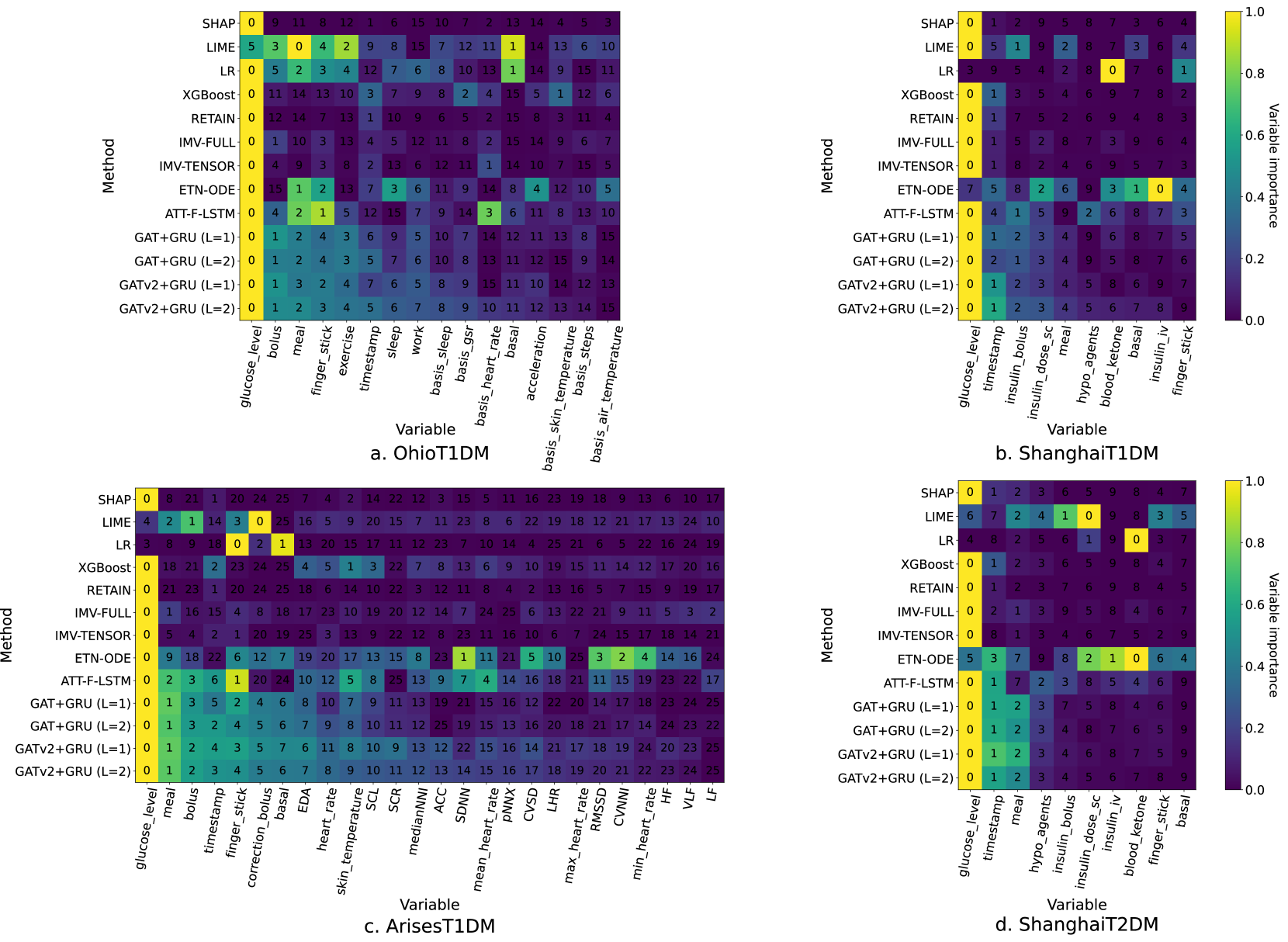
After seeing the variable ranking lists w.r.t. in four datasets in Figure 3, we have the observations as follows:
1) The target variable, “glucose_level”, should be the most important in BGLP [44, 11]. GARNNs, ATT-F-LSTM, IMV-LSTMs, RETAIN, XGBoost and SHAP can consistently focus on the target variable, while the rest methods often lose focus.
2) GARNNs typically outperform baseline models by assigning significant importance to “timestamp” in the rankings, particularly for Shanghai T1DM and T2DM where the sample frequency of CGM is relatively low. This characteristic aligns with clinical observations that BG fluctuations are linked to personal lifestyles, exhibiting distinct temporal patterns. It is significant that useful exogenous variables are highlighted when lacking enough values from the target variable in Shanghai datasets.
3) Given that we predict the future BG of CGM instead of “finger_stick”, i.e., capillary BG test, more difference between them may reduce the importance of “finger_stick”. The MAE between “glucose_level” and “finger_stick” in OhioT1DM and AriseT1DM is lower, i.e., 20.92 and 9.97 mg/dL, respectively. The MAE between them in ShanghaiT1DM and ShanghaiT2DM are respectively 29.03 and 22.31 mg/dL. Hence, GARNNs give special highlights to “finger_stick” in OhioT1DM and AriseT1DM but less importance in ShanghaiT1DM and ShanghaiT2DM because of the larger MAE, while the variable importance ranking of other methods does not have similar observations.
4) Apart from “glucose_level”, “finger_stick” and “timestamp”, both bolus insulin (“bolus”, “correction_bolus”, “insulin_dose_sc” and “insulin_bolus”) and carbohydrate intake (“meal”) should be important variables as well, because they can rapidly affect the BG levels within short periods. Basal insulin (“basal”), also called “background insulin”, steadily controls BG levels for long periods. Besides, “insulin_iv” is an intravenous insulin infusion for super serious hyperglycemia under some extreme circumstances.
Therefore, in terms of daily cases, bolus insulin tends to be more important than basal insulin in BGLP. GARNNs follow this knowledge in four datasets, while other methods fail to do that. Besides, in ArisesT1DM, GARNNs give “bolus” more importance than “correction_bolus”, because the latter is an extra insulin taken during hyperglycemia. The amount of the latter is much less than the former.
On the other hand, a predominant reason for T2DM is that cells respond inactively to insulin. Hence, compared with the variable ranking in ShanghaiT1DM, GARNNs reduce the importance of bolus insulin and give more importance to “meal” and non-insulin hypoglycemic agents, “hypo_agents”, in ShanghaiT2DM.
5) In OhioT1DM, the self-reported events, i.e., “exercise” and “sleep”, should be more important than the sensor data, e.g., “basis_heart_rate”, “basis_gsr”, etc. This is because both exercising and sleeping can indirectly cause changes in BG levels. Unlike the other methods, “GATv2+GRU” reflects this knowledge. Besides, “sleep” and “basis_sleep” are self-reported and sensor-detected, respectively, but “basis_sleep” misses of the sleeping intensity data, so GARNNs give more importance to “sleep”.
6) In the analysis of the number of layers in GAT or GATv2, it is observed that this can slightly alter the ranking of variable importance . For instance, different configurations like “GATv2+GRU()” show varying importance rankings for variables like “sleep” and “work”. This was further substantiated by a feature ablation study in OhioT1DM [45], indicating that “sleep” improves prediction accuracy more than “work”. The preference for “sleep” by “GATv2+GRU()” seems more aligned with these findings, suggesting that multiple layers in GATv2 might capture more detailed interactions among variables. Similarly, there are subtle differences in rankings between GAT and GATv2, with GAT-based methods favoring “work” over “sleep”. It is hypothesized that GAT’s slightly lesser interpretability might be linked to its relatively weaker prediction performance, as indicated in tables 1-4.
Despite these variations, both models consistently classify variables into categories like most important, very important, somewhat important, and less important. For example, both models consistently identify “glucose_level” as the most important variable across all datasets. This is followed by other closely related and significant variables that have a direct impact on BG levels, such as carbohydrate intake, classified as very important. Subsequently, both models also pay attention to variables that indirectly affect BG levels, like exercise in the OhioT1DM dataset. These are considered somewhat important variables. Finally, both GAT and GATv2 place other less significant variables at the lower end of the ranking.
7) Based on Theorem 3, the gaps between the prediction and the calculation of variable importance are affected by . Figure 4 shows the variable importance ranking of GARNNs when changing . We find that the gaps cannot significantly alter the variable importance, especially for “GATv2+RNN”. Even with different gap sizes, the changes in variable importance remain small but still acceptable.
5.6 Interpretation of feature maps
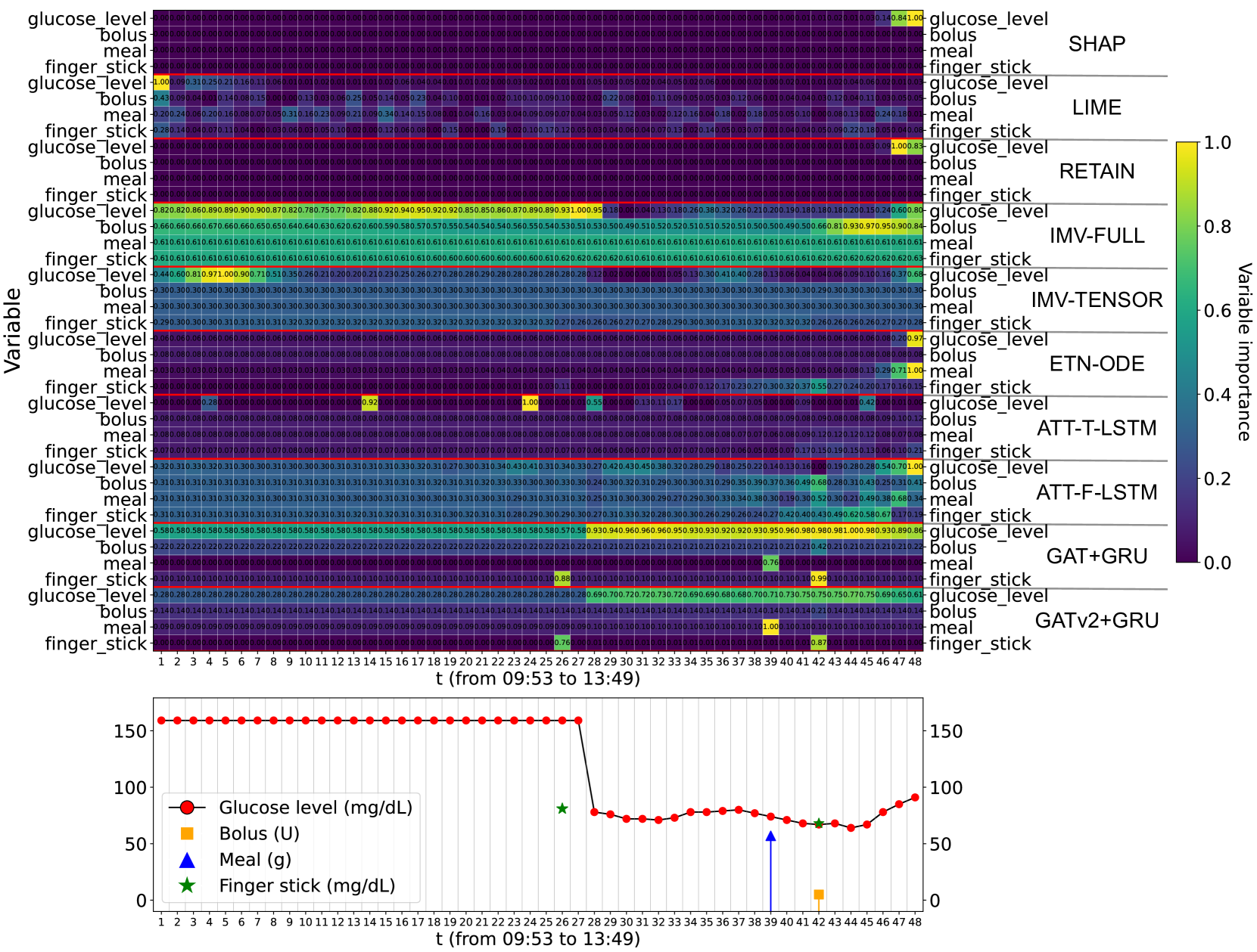
CGM might be inaccurate after being worn for a period, so calibration by “finger_stick” can make it back to normal. According to the bottom sub-figure of Figure 5, participant 591 finds the CGM is unreliable, so this patient takes the first “finger_stick” at . Then, this patient calibrates “glucose_level” of CGM with “finger_stick”, and “glucose_level” goes down and back to accurate measurements after . Next, this patient has a meal at ; this patient takes “bolus” and another “finger_stick” at .
Hence, “glucose_level” () should be more important than “glucose_level” (). Based on the feature maps of the methods, GARNNs accurately highlight the importance of “glucose_level” (). Furthermore, GARNNs exactly capture the sparse signals, i.e., “bolus”, “meal” and “finger_stick”, considering the related cells are markedly brighter when . Besides, GARNNs precisely focus on the lowest BG level, when . However, the feature maps of other methods are not quite informative. All of them cannot explicitly show the usage of sparse signals. Meanwhile, they fail to focus “glucose_level” time series reasonably.
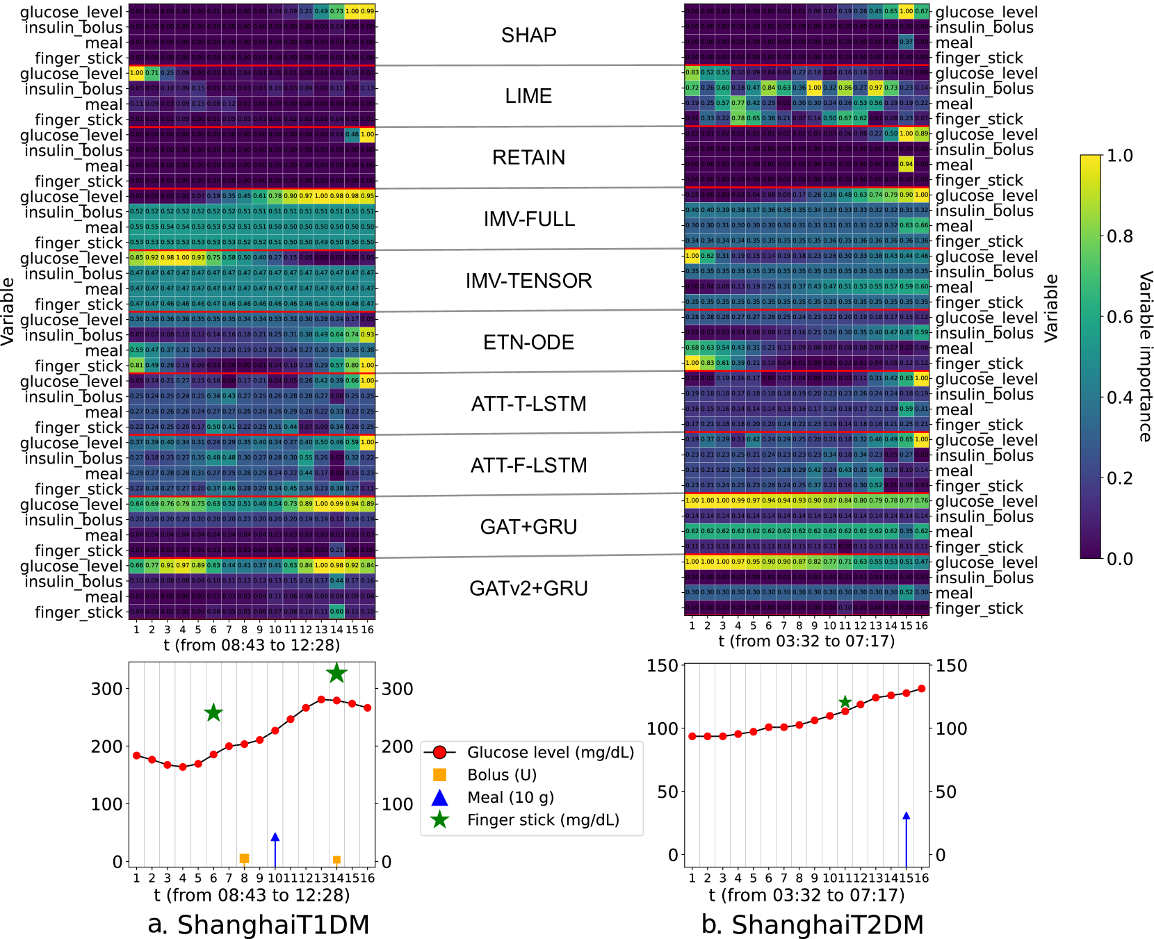
More feature maps are shown in Figure 6. Note that the “meal” in ShanghaiT1DM or ShanghaiT2DM means the amount of food intake rather than carbohydrate intake. The variable importance is scaled to as well. The observations still hold that GARNNs () can correctly focus the important values of “glucose_level”, i.e., and in Figure 6a, and in Figure 6b. Important sparse signals gain more attention as well, i.e., in Figure 6a, and in Figure 6b.
6 Conclusion
In this work, we propose GARNNs, novel interpretable models, by incorporating graph attention networks and RNNs for BGLP. One notable advantage of GARNNs is their ability to provide significant variable importance for ranking variables and generating feature maps. In the experiments on four datasets, GARNNs demonstrate superior performance when compared with twelve baseline models. GARNNs outperform the baselines in both the accuracy of predictions and the quality of explanations regarding the contribution of variables.
The main limitation of this work is its narrow focus, primarily concentrating on specific aspects of BG management without extensively exploring other relevant scenarios, such as the development of interpretable models for insulin advice. Consequently, future work will aim to expand the applicability of the proposed interpretable models across a broader range of BG management scenarios.
7 Acknowledgement
We thank the support from UKRI Center for Doctoral Training in AI-enabled healthcare systems [EP/S021612/1] and University College London Overseas Research Scholarships. We also appreciate the support from Rosetrees Trust (Grant number: UCL-IHE-2020\102) and Great Ormond Street Hospital (Charity ref.X12018). The study sponsors had no study involvement.
References
- WHO [2023] WHO, Diabetes, https://www.who.int/health-topics/diabetes, 2023. Accessed: 2023-12-19.
- Bloomgarden [2004] Z. T. Bloomgarden, Diabetes Complications , Diabetes Care 27 (2004) 1506–1514. doi:10.2337/diacare.27.6.1506.
- Mora et al. [2023] T. Mora, D. Roche, B. Rodríguez-Sánchez, Predicting the onset of diabetes-related complications after a diabetes diagnosis with machine learning algorithms, Diabetes Research and Clinical Practice 204 (2023) 110910. doi:10.1016/j.diabres.2023.110910.
- Woldaregay et al. [2019] A. Z. Woldaregay, E. Årsand, S. Walderhaug, D. J. Albers, L. Mamykina, T. Botsis, G. Hartvigsen, Data-driven modeling and prediction of blood glucose dynamics: Machine learning applications in type 1 diabetes, Artificial Intelligence in Medicine 98 (2019) 109–134. doi:10.1016/J.ARTMED.2019.07.007.
- Bezerra et al. [2023] M. F. Bezerra, C. Neves, J. S. Neves, D. Carvalho, Time in range and complications of diabetes: a cross-sectional analysis of patients with type 1 diabetes, Diabetology & Metabolic Syndrome 15 (2023) 244. doi:10.1186/s13098-023-01219-2.
- Plis et al. [2014] K. Plis, R. C. Bunescu, C. Marling, J. Shubrook, F. Schwartz, A machine learning approach to predicting blood glucose levels for diabetes management, in: AAAI Workshop’14, volume WS-14-08, 2014.
- Cichosz et al. [2021] S. L. Cichosz, T. Kronborg, M. H. Jensen, O. K. Hejlesen, Penalty weighted glucose prediction models could lead to better clinically usage, Comput. Biol. Medicine 138 (2021) 104865. doi:10.1016/J.COMPBIOMED.2021.104865.
- Nemat et al. [2023] H. Nemat, H. Khadem, J. Elliott, M. Benaissa, Causality analysis in type 1 diabetes mellitus with application to blood glucose level prediction, Comput. Biol. Medicine 153 (2023) 106535. doi:10.1016/J.COMPBIOMED.2022.106535.
- Zhu et al. [2023a] T. Zhu, L. Kuang, J. Daniels, P. Herrero, K. Li, P. Georgiou, Iomt-enabled real-time blood glucose prediction with deep learning and edge computing, IEEE Internet of Things Journal 10 (2023a) 3706–3719. doi:10.1109/JIOT.2022.3143375.
- Zhu et al. [2023b] T. Zhu, K. Li, P. Herrero, P. Georgiou, Personalized blood glucose prediction for type 1 diabetes using evidential deep learning and meta-learning, IEEE Trans. Biomed. Eng. 70 (2023b) 193–204. doi:10.1109/TBME.2022.3187703.
- Zhu et al. [2022] T. Zhu, C. Uduku, K. Li, P. Herrero, N. Oliver, P. Georgiou, Enhancing self-management in type 1 diabetes with wearables and deep learning, npj Digital Medicine 5 (2022) 78. doi:10.1038/S41746-022-00626-5.
- Karim et al. [2020] R. A. H. Karim, I. Vassányi, I. Kósa, After-meal blood glucose level prediction using an absorption model for neural network training, Comput. Biol. Medicine 125 (2020) 103956. doi:10.1016/J.COMPBIOMED.2020.103956.
- Ancona et al. [2018] M. Ancona, E. Ceolini, C. Öztireli, M. Gross, Towards better understanding of gradient-based attribution methods for deep neural networks, in: ICLR’18, 2018.
- Guo et al. [2019] T. Guo, T. Lin, N. Antulov-Fantulin, Exploring interpretable LSTM neural networks over multi-variable data, in: ICML’19, volume 97, 2019, pp. 2494–2504.
- Lundberg and Lee [2017] S. M. Lundberg, S. Lee, A unified approach to interpreting model predictions, in: NIPS’17, 2017, pp. 4765–4774.
- Hochreiter and Schmidhuber [1997] S. Hochreiter, J. Schmidhuber, Long short-term memory, Neural Comput. 9 (1997) 1735–1780. doi:10.1162/NECO.1997.9.8.1735.
- Cappon et al. [2020] G. Cappon, L. Meneghetti, F. Prendin, J. Pavan, G. Sparacino, S. D. Favero, A. Facchinetti, A personalized and interpretable deep learning based approach to predict blood glucose concentration in type 1 diabetes, in: KDH@ECAI’20, volume 2675, 2020, pp. 75–79.
- Prendin et al. [2023] F. Prendin, J. Pavan, G. Cappon, S. Del Favero, G. Sparacino, A. Facchinetti, The importance of interpreting machine learning models for blood glucose prediction in diabetes: an analysis using shap, Scientific Reports 13 (2023) 16865. doi:10.1038/s41598-023-44155-x.
- Ribeiro et al. [2016] M. T. Ribeiro, S. Singh, C. Guestrin, "why should I trust you?": Explaining the predictions of any classifier, in: ACM KDD’16, 2016, pp. 1135–1144. doi:10.1145/2939672.2939778.
- Choi et al. [2016] E. Choi, M. T. Bahadori, J. Sun, J. Kulas, A. Schuetz, W. F. Stewart, RETAIN: an interpretable predictive model for healthcare using reverse time attention mechanism, in: NIPS’16, 2016, pp. 3504–3512.
- Gao et al. [2023] P. Gao, X. Yang, R. Zhang, K. Huang, J. Y. Goulermas, Explainable tensorized neural ordinary differential equations for arbitrary-step time series prediction, IEEE Trans. Knowl. Data Eng. 35 (2023) 5837–5850. doi:10.1109/TKDE.2022.3167536.
- Gandin et al. [2021] I. Gandin, A. Scagnetto, S. Romani, G. Barbati, Interpretability of time-series deep learning models: A study in cardiovascular patients admitted to intensive care unit, Journal of Biomedical Informatics 121 (2021) 103876. doi:10.1016/j.jbi.2021.103876.
- Brody et al. [2022] S. Brody, U. Alon, E. Yahav, How attentive are graph attention networks?, in: ICLR’22, 2022.
- Cho et al. [2014] K. Cho, B. van Merrienboer, D. Bahdanau, Y. Bengio, On the properties of neural machine translation: Encoder-decoder approaches, in: SSST@EMNLP’14, 2014, pp. 103–111. doi:10.3115/V1/W14-4012.
- Velickovic et al. [2018] P. Velickovic, G. Cucurull, A. Casanova, A. Romero, P. Liò, Y. Bengio, Graph attention networks, in: ICLR’18, 2018.
- Shrikumar et al. [2017] A. Shrikumar, P. Greenside, A. Kundaje, Learning important features through propagating activation differences, in: ICML’17, volume 70, 2017, pp. 3145–3153.
- Bykov et al. [2022] K. Bykov, A. Hedström, S. Nakajima, M. M. Höhne, Noisegrad - enhancing explanations by introducing stochasticity to model weights, in: AAAI’22, 2022, pp. 6132–6140. doi:10.1609/AAAI.V36I6.20561.
- Tonekaboni et al. [2020] S. Tonekaboni, S. Joshi, K. Campbell, D. K. Duvenaud, A. Goldenberg, What went wrong and when? instance-wise feature importance for time-series black-box models, in: NIPS’20, volume 33, 2020, pp. 799–809.
- Kwon and Zou [2022] Y. Kwon, J. Y. Zou, Weightedshap: Analyzing and improving shapley based feature attributions, in: NIPS’22, volume 35, 2022, pp. 34363–34376.
- Rajapaksha and Bergmeir [2022] D. Rajapaksha, C. Bergmeir, LIMREF: local interpretable model agnostic rule-based explanations for forecasting, with an application to electricity smart meter data, in: AAAI’22, 2022, pp. 12098–12107. doi:10.1609/AAAI.V36I11.21469.
- Chu et al. [2020] Y. Chu, X. Wang, J. Ma, K. Jia, J. Zhou, H. Yang, Inductive granger causal modeling for multivariate time series, in: ICDM’20, 2020, pp. 972–977.
- Shamout et al. [2020] F. E. Shamout, T. Zhu, P. Sharma, P. J. Watkinson, D. A. Clifton, Deep interpretable early warning system for the detection of clinical deterioration, IEEE J. Biomed. Health Informatics 24 (2020) 437–446. doi:10.1109/JBHI.2019.2937803.
- Aguiar et al. [2022] H. Aguiar, M. D. Santos, P. J. Watkinson, T. Zhu, Learning of cluster-based feature importance for electronic health record time-series, in: ICML’22, volume 162, 2022, pp. 161–179.
- Hsieh et al. [2021] T. Hsieh, S. Wang, Y. Sun, V. G. Honavar, Explainable multivariate time series classification: A deep neural network which learns to attend to important variables as well as time intervals, in: ACM WSDM’21, 2021, pp. 607–615. doi:10.1145/3437963.3441815.
- Xu et al. [2018] Y. Xu, S. Biswal, S. R. Deshpande, K. O. Maher, J. Sun, RAIM: recurrent attentive and intensive model of multimodal patient monitoring data, in: ACM KDD’18, 2018, pp. 2565–2573. doi:10.1145/3219819.3220051.
- Kaji et al. [2019] D. A. Kaji, J. R. Zech, J. S. Kim, S. K. Cho, N. S. Dangayach, A. B. Costa, E. K. Oermann, An attention based deep learning model of clinical events in the intensive care unit, PloS one 14 (2019) e0211057. doi:10.1371/journal.pone.0211057.
- Zhao et al. [2023] Q. Zhao, J. Zhu, X. Shen, C. Lin, Y. Zhang, Y. Liang, B. Cao, J. Li, X. Liu, W. Rao, et al., Chinese diabetes datasets for data-driven machine learning, Scientific Data 10 (2023) 35. doi:10.1038/s41597-023-01940-7.
- Marling and Bunescu [2020] C. Marling, R. C. Bunescu, The ohiot1dm dataset for blood glucose level prediction: Update 2020, in: KDH@ECAI’20, volume 2675, 2020, pp. 71–74.
- Pedregosa et al. [2011] F. Pedregosa, G. Varoquaux, A. Gramfort, V. Michel, B. Thirion, O. Grisel, M. Blondel, P. Prettenhofer, R. Weiss, V. Dubourg, J. Vanderplas, A. Passos, D. Cournapeau, M. Brucher, M. Perrot, E. Duchesnay, Scikit-learn: Machine learning in Python, Journal of Machine Learning Research 12 (2011) 2825–2830. doi:10.5555/1953048.2078195.
- Chen and Guestrin [2016] T. Chen, C. Guestrin, XGBoost: A scalable tree boosting system, in: ACM KDD’16, 2016, pp. 785–794. doi:10.1145/2939672.2939785.
- Oreshkin et al. [2020] B. N. Oreshkin, D. Carpov, N. Chapados, Y. Bengio, N-BEATS: neural basis expansion analysis for interpretable time series forecasting, in: ICLR’20, 2020.
- Challu et al. [2023] C. Challu, K. G. Olivares, B. N. Oreshkin, F. G. Ramírez, M. M. Canseco, A. Dubrawski, NHITS: neural hierarchical interpolation for time series forecasting, in: AAAI’23, 2023, pp. 6989–6997. doi:10.1145/2939672.2939778.
- Favero et al. [2012] S. D. Favero, A. Facchinetti, C. Cobelli, A glucose-specific metric to assess predictors and identify models, IEEE Trans. Biomed. Eng. 59 (2012) 1281–1290. doi:10.1109/TBME.2012.2185234.
- Bevan and Coenen [2020] R. Bevan, F. Coenen, Experiments in non-personalized future blood glucose level prediction, in: KDH@ECAI’20, volume 2675, 2020, pp. 100–104.
- Piao and Li [2023] C. Piao, K. Li, Blood glucose level prediction: A graph-based explainable method with federated learning, CoRR abs/2312.12541 (2023). doi:10.48550/ARXIV.2312.12541. arXiv:2312.12541.