Scaling Robust Optimization for Multi-Agent Robotic Systems: A Distributed Perspective

Abstract

This paper presents a novel distributed robust optimization scheme for steering distributions of multi-agent systems under stochastic and deterministic uncertainty. Robust optimization is a subfield of optimization which aims in discovering an optimal solution that remains robustly feasible for all possible realizations of the problem parameters within a given uncertainty set. Such approaches would naturally constitute an ideal candidate for multi-robot control, where in addition to stochastic noise, there might be exogenous deterministic disturbances. Nevertheless, as these methods are usually associated with significantly high computational demands, their application to multi-agent robotics has remained limited. The scope of this work is to propose a scalable robust optimization framework that effectively addresses both types of uncertainties, while retaining computational efficiency and scalability. In this direction, we provide tractable approximations for robust constraints that are relevant in multi-robot settings. Subsequently, we demonstrate how computations can be distributed through an Alternating Direction Method of Multipliers (ADMM) approach towards achieving scalability and communication efficiency. Simulation results highlight the performance of the proposed algorithm in effectively handling both stochastic and deterministic uncertainty in multi-robot systems. The scalability of the method is also emphasized by showcasing tasks with up to 100 agents. The results of this work indicate the promise of blending robust optimization, distribution steering and distributed optimization towards achieving scalable, safe and robust multi-robot control.

I Introduction

Multi-agent optimization and control problems are emerging increasingly often in a vast variety of robotics applications such as multi-vehicle coordination [16, 43], swarm robotics [37], cooperative manipulation [13] and others. As the size and complexity of such systems has been rapidly escalating, a substantial requirement for developing scalable and distributed algorithms for tackling these problems has been developing as well [35, 38, 46]. In the meantime, accompanying such algorithms with safety and robustness guarantees in environments with substantial levels of uncertainty is also a highly desirable attribute for securing the safe operation of all agents.

Uncertainty has been primarily modeled as stochastic noise in a significant portion of the multi-agent control literature. Some indicative approaches involve multi-agent LQG control [1, 24, 39], distributed covariance steering [33, 34], multi-agent path integral control [14, 42] and learning-based stochastic optimal control methods [21, 26], among others. Nevertheless, such approaches would typically fall short in scenarios where the underlying disturbances might be exogenous interventions, environmental factors, modelling inaccuracies, etc., that cannot be properly represented as stochastic signals [5]. Such problems create the necessity of finding robust optimal policies that would guarantee feasibility for all possible values of such disturbances within some bounds.

Robust optimization is a subfield of optimization that addresses the problem of discovering an optimal solution that remains robust feasible for all possible realizations of the problem parameters within a given uncertainty set [5, 6]. Although robust optimization has found significant successful applications in many areas such as power systems [8], supply chain networks [29], communication systems [10], etc., there have only been limited attempts for addressing problems relevant to robotics [19, 23, 30, 40]. The field of robust control is a also closely related area with long history in addressing disturbances from predefined sets [12, 45]. However, as this area is mainly focused on synthesis techniques for stabilization and performance maintenance, merging such methods with distributed optimization and steering state distributions for multi-agent systems is not as straightforward. On the contrary, as robust optimization allows for more flexibility in designing such approaches, the current work is focused on leveraging the latter for safe multi-agent control.

Another promising area that has recently emerged in the context of safe stochastic control is the one of steering the state distributions of systems under predefined target distributions - mostly known as covariance steering [3, 11, 22]. Such methods have found several successful applications in path planning [25], trajectory optimization [4, 44], robotic manipulation [20], flight control [7, 31], multi-robot control [33, 34] and others. More recently, a convex optimization framework for steering state distributions and effectively addressing both stochastic noise and bounded deterministic disturbances was presented [19]. In a similar direction, a data-driven robust optimization-based method was recently proposed in [28], including estimating the noise realization from collected data. Nevertheless, as such approaches result in high-dimensional semidefinite programming (SDP) problems, the computational demands for addressing multi-agent control tasks have remained prohibitive.

The scope of this work is to provide a scalable robust optimization framework for steering distributions of multi-agent systems to specific targets under stochastic and deterministic uncertainty. Towards this direction, we present a distributed algorithm for safe and robust multi-robot control whose effectiveness and scalability are verified through simulation experiments. The specific contributions of this paper can be listed as follows.

• We combine elements from the areas of robust optimization, distribution steering and distributed computation architectures for deriving a scalable and robust approach for multi-agent control. To our best knowledge, this is the first work to fuse these areas into a single methodology.

• We circumvent computational expensiveness by providing tractable approximations of robust optimization constraints that are relevant for multi-robot control problems.

• We present a distributed algorithm based on an Alternating Direction Method of Multipliers (ADMM) approach for multi-agent robust distribution steering.

• We provide simulation results that demonstrate the effectiveness of the proposed algorithm in handling stochastic and deterministic uncertainty. The scalability of the method is also highlighted by showing multi-robot tasks with up to 100 agents.

The remaining of this paper is organized as follows. In Section II, we state the multi-agent problem to be considered in this work. The proposed distributed robust optimization framework is presented in Section III. An analysis of performance and scalability is demonstrated through simulation experiments in Section IV. Finally, the conclusion of this paper, as well as future research directions, are provided in Section V.

II Problem Statement

In this section, we present the multi-agent robust optimization problem to be addressed in this work. Initially, we familiarize the reader with the notation used throughout this paper. Subsequently, we present the basic multi-agent problem setup and the dynamics of the agents. The two main characterizations of underlying uncertainty, i.e., deterministic and stochastic, are then formulated. Then, we specify the control policies of the agents and the robust constraints that are considered in our framework. Finally, the exact formulation of the multi-agent problem is provided.

II-A Notation

The integer set $[a,b]\cap\mathbb{Z}$ is denoted with $\llbracket a,b\rrbracket$. The space of matrices ${\bf X}\in\mathbb{R}^{n\times n}$ that are symmetric positive (semi)-definite, i.e., ${\bf X}\succ 0$ (${\bf X}\succeq 0$) is denoted with $\mathbb{S}_{n}^{++}$ ($\mathbb{S}_{n}^{+}$). The inner product of two vectors ${\bm{x}},{\bm{y}}\in\mathbb{R}^{n}$ is denoted with $\langle{\bm{x}},{\bm{y}}\rangle={\bm{x}}^{\mathrm{T}}{\bm{y}}$. The $\ell_{2}$-norm of a vector ${\bm{x}}=\begin{bmatrix}x_{1}&\dots&x_{n}\end{bmatrix}\in\mathbb{R}^{n},$ is defined as $\|{\bm{x}}\|_{2}=\sqrt{\langle{\bm{x}},{\bm{x}}\rangle}$. The weighted norm $\|{\bm{x}}\|_{{\bf Q}}=\|{\bm{Q}}^{1/2}{\bm{x}}\|_{2}=\sqrt{{\bm{x}}^{\mathrm{T}}{\bm{Q}}{\bm{x}}}$ is also defined for any ${\bf Q}\in\mathbb{S}_{n}^{++}$. In addition, the Frobenius norm of a matrix ${\bf X}\in\mathbb{R}^{m\times n}$ is given by $\|{\bf X}\|_{F}=\sqrt{\mathrm{tr}({\bf X}^{\mathrm{T}}{\bf X})}$. With $[{\bm{x}}_{1};\dots;{\bm{x}}_{n}]$, we denote the vertical concatenation of a series of vectors ${\bm{x}}_{1},\dots,{\bm{x}}_{n}$. Furthermore, the probability of an event $\pazocal{A}$ is denoted with $\mathbb{P}(\pazocal{A})$. Given a random variable (r.v.) ${\bm{x}}\in\mathbb{R}^{n}$, its expectation and covariance are denoted with $\mathbb{E}[x]\in\mathbb{R}^{n}$ and $\mathrm{Cov}({\bm{x}})\in\mathbb{S}_{n}^{+}$, respectively. The cardinality of a set $\pazocal{X}$ is denoted as $n(\pazocal{X})$. Finally, given a set $\pazocal{X}$, the indicator function $\pazocal{I}_{\pazocal{X}}$ is defined as $\pazocal{I}_{\pazocal{X}}(x)=0$, if $x\in\pazocal{X}$, and $\pazocal{I}_{\pazocal{X}}(x)=+\infty$, otherwise.

II-B Problem Setup

Let us consider a multi-agent system of $N$ agents defined by the set $\pazocal{V}=\{1,\dots,N\}$. All agents $i\in\pazocal{V}$ may be subject to diverse dynamics, inter-agent interactions, and exogenous deterministic and stochastic uncertainty. Each agent $i\in\pazocal{V}$ has a set of neighbors defined by $\pazocal{N}_{i}\subseteq\pazocal{V}$. Furthermore, for each agent $i\in\pazocal{V}$, we define the set of agents that consider $i$ as a neighbor through $\pazocal{P}_{i}=\{j\in\pazocal{V}|i\in\pazocal{N}_{j}\}$.

II-C Dynamics

We consider the following discrete-time linear time-varying dynamics for each agent $i\in\pazocal{V}$,

$$x_{k+1}^{i}=A_{k}^{i}x_{k}^{i}+B_{k}^{i}u_{k}^{i}+C_{k}^{i}d_{k}^{i}+D_{k}^{i}w_{k}^{i},~{}k\in\llbracket 0,T-1\rrbracket,$$ (1)

where $x_{k}^{i}\in\mathbb{R}^{n_{x_{i}}}$ is the state, $u_{k}^{i}\in\mathbb{R}^{n_{u_{i}}}$ is the control input of agent $i$ at time $k$, and $T$ is the time horizon. The terms $d_{k}^{i}\in\mathbb{R}^{n_{d_{i}}}$ represent exogenous deterministic disturbances, while the terms $w_{i}^{k}\in\mathbb{R}^{n_{w_{i}}}$ refer to stochastic disturbances, with their exact mathematical representations presented in Section II-D. Each initial state $x_{0}^{i},~{}i\in\pazocal{V}$, is of the following form

$$x_{0}^{i}=\bar{x}_{0}^{i}+\bar{d}_{0}^{i}+s_{0}^{i},$$ (2)

where $\bar{x}_{0}^{i}$ is the known part, while $\bar{d}_{0}^{i}$ and $s_{0}^{i}$ refer to the unknown exogenous deterministic and stochastic parts, respectively. Finally, $A_{k}^{i},B_{k}^{i},C_{k}^{i},D_{k}^{i}$ are the dynamics matrices of appropriate dimensions.

For convenience, let us also define the sequences ${\bm{x}}^{i}=[x_{0}^{i};\dots;x_{T}^{i}]\in\mathbb{R}^{(T+1)n_{x_{i}}}$, ${\bm{u}}^{i}=[u_{0}^{i};\dots;u_{T-1}^{i}]$ $\in\mathbb{R}^{Tn_{u_{i}}}$, ${\bm{w}}^{i}=[s_{0}^{i};w_{0}^{i};\dots;w_{T-1}^{i}]\in\mathbb{R}^{n_{x_{i}}+Tn_{w_{i}}}$ and $\bm{\zeta}^{i}=[\bar{d}_{0}^{i};d_{0}^{i};\dots;d_{T-1}^{i}]\in\mathbb{R}^{n_{x_{i}}+Tn_{d_{i}}}$. The dynamics (1) can then be rewritten in a more compact form as

$${\bm{x}}^{i}={\bf G}_{0}^{i}\bar{x}_{0}^{i}+{\bf G}_{u}^{i}{\bm{u}}^{i}+{\bf G}_{{\bm{w}}}^{i}\bm{{\bm{w}}}^{i}+{\bf G}_{\zeta}^{i}\bm{\zeta}^{i},$$ (3)

where the matrices ${\bf G}_{0}^{i},{\bf G}_{u}^{i},{\bf G}_{{\bm{w}}}^{i},{\bf G}_{\zeta}^{i}$ are provided in Section I of the Supplementary Material (SM).

II-D Characterizations of Uncertainty

As previously mentioned, we consider the existence of both exogenous deterministic and stochastic uncertainties. These two types of uncertainty are formally described as follows.

Exogenous deterministic uncertainty

The unknown deterministic disturbances $\bm{\zeta}^{i}$ typically stem from external factors that cannot be accurately represented through stochastic signals. This creates a requirement to formulate optimization problems and achieve optimal policies that are feasible in a robust sense for all possible values of such disturbances in a bounded uncertainty set. Examples of such uncertainty sets include ellipsoids, polytopes, and others [5]. In this work, we assume the sequence $\bm{\zeta}^{i}$ to be lying inside an ellipsoidal uncertainty set defined as follows

$$\pazocal{U}_{i}[\tau^{i}]=\big{\{}\bm{\zeta}^{i}\in\mathbb{R}^{n_{\zeta_{i}}} |\;\exists({\bm{z}}_{i}\in\mathbb{R}^{\bar{n}_{i}},\tau^{i}\in\mathbb{R}):\;$$ (4)

$$\bm{\zeta}^{i}=\bm{\Gamma}_{i}{\bm{z}}_{i},\;\langle{\bf S}_{i}{\bm{z}}_{i},{\bm{z}}_{i}\rangle\leq\tau^{i}\big{\}},$$

where $n_{\zeta_{i}}=n_{x_{i}}+Tn_{d_{i}}$, $\bm{\Gamma}_{i}\in\mathbb{R}^{n_{\zeta_{i}}\times\bar{n}_{i}}$, ${\bf S}_{i}\in\mathbb{S}_{++}^{\bar{n}_{i}}$ and $\tau^{i}>0$ is the uncertainty level. Ellipsoidal sets are used to model uncertainty in various robust control applications [27]. Further, ellipsoid sets have simple geometric structure, and more complex sets can be approximated using ellipsoids.

Stochastic uncertainty

The unknown stochastic component ${\bm{w}}^{i}$ is assumed to be a Gaussian random vector with mean ${\bm{\mu}}_{{{\bm{w}}}^{i}}=\mathbb{E}[{\bm{w}}^{i}]=0$, and covariance ${\bm{\Sigma}}_{\bm{{\bm{w}}}^{i}}=\mathrm{Cov}[{\bm{w}}^{i}]$.

II-E Control Policies

Towards addressing both types of uncertainty, we consider affine purified state feedback policies [5, 19] for all agents. Let us first introduce the disturbance-free states $\hat{x}_{k}^{i}$, whose dynamics are given by

$$\hat{x}_{k+1}^{i} =A_{k}^{i}\hat{x}_{t}^{i}+B_{k}^{i}u_{k}^{i},\quad k\in\llbracket 0,T-1\rrbracket,$$ (5)

$$\hat{x}_{0}^{i} =\bar{x}_{0}^{i}.$$ (6)

Subsequently, we can define the purified states $\delta_{k}^{i}=x_{k}^{i}-\hat{x}_{k}^{i}$, whose dynamics are given by

$$\delta_{k+1}^{i} =A_{k}^{i}\delta_{k}^{i}+C_{k}^{i}d_{k}^{i}+D_{k}^{i}w_{k}^{i}\quad k\in\llbracket 0,T-1\rrbracket,$$ (7)

$$\delta_{0}^{i} =\bar{d}_{0}^{i}+s_{0}^{i},$$

or more compactly by

$${\bm{\delta}}^{i}={\bf G}_{{\bm{w}}}^{i}\bm{{\bm{w}}}^{i}+{\bf G}_{\zeta}^{i}\bm{\zeta}^{i},$$ (8)

where ${\bm{\delta}}^{i}=\begin{bmatrix}{\bm{\delta}}_{0}^{i};&\dots;&{\bm{\delta}}_{T}^{i}\end{bmatrix}$. We consider the following affine purified state feedback control policy for each agent $i$,

$$u^{i}_{k}=\bar{u}^{i}_{k}+\sum_{\ell=0}^{k}K^{i}_{k,\ell}\delta^{i}_{\ell},\;\forall\;k\in\llbracket 0,T-1\rrbracket,$$ (9)

where $\bar{u}^{i}_{k}\in\mathbb{R}^{n_{u_{i}}}$ are the feed-forward control inputs and $K^{i}_{k,\ell}\in\mathbb{R}^{n_{u_{i}}\times n_{x_{i}}}$ are feedback gains on the purified states. The above policies can be written in compact form as

$${\bm{u}}^{i}=\bar{{\bm{u}}}^{i}+{\bf K}^{i}{\bm{\delta}}^{i},$$ (10)

where

$$\bar{{\bm{u}}}^{i}=\begin{bmatrix}\bar{u}_{0}^{i};&\dots;&\bar{u}_{T-1}^{i}\end{bmatrix},$$

$${\bf K}^{i}=\begin{bmatrix}K_{0,0}^{i}&{\bf 0}&\dots&{\bf 0}&{\bf 0}\\ K_{1,0}^{i}&K_{1,1}^{i}&\dots&{\bf 0}&{\bf 0}\\ \vdots&\vdots&\vdots&\vdots&\vdots\\ K_{T-1,0}^{i}&K_{T-1,1}^{i}&\dots&K_{T-1,T-1}^{i}&{\bf 0}\end{bmatrix}.$$

II-F Robust Constraints

Next, we introduce the types of constraints that are considered in this work. We highlight that the following constraints must be satisfied robustly for all possible values of ${\bm{\zeta}}^{i}$ lying inside the uncertainty sets $\pazocal{U}_{i},\ i\in\pazocal{V}$.

Robust linear mean constraints

The first class of constraints we consider are robust linear constraints on the expectation of the state sequence ${\bm{x}}^{i}$ of agent $i\in\pazocal{V}$,

$${\bf A}_{i}\mathbb{E}[{\bm{x}}^{i}]\leq\bm{b}_{i},\quad\forall{\bm{\zeta}}^{i}\in\pazocal{U}_{i},$$ (11)

where ${\bf A}_{i}\in\mathbb{R}^{m\times n_{x_{i}}}$, $\bm{b}_{i}\in\mathbb{R}^{m}$. In a robotics setting, such constraints could typically represent bounds on the mean position, velocity, etc.

Robust nonconvex norm-of-mean constraints

Furthermore, we consider nonconvex inequality constraints of the form

$$\|{\bf A}_{i}\mathbb{E}[x_{k}^{i}]-\bm{b}_{i}\|_{2}\geq c_{i},\quad\forall{\bm{\zeta}}^{i}\in\pazocal{U}_{i},$$ (12)

where ${\bf A}_{i}\in\mathbb{R}^{m\times n_{x_{i}}}$, $\bm{b}_{i}\in\mathbb{R}^{m}$, $c_{i}\in\mathbb{R}^{+}$. Such constraints are typically useful for capturing avoiding obstacles, forbidden regions, etc. In addition, we extend to the inter-agent version of these constraints which is given by

$$\|{\bf A}_{i}\mathbb{E}[{\bm{x}}^{i}_{k}]-{\bf A}_{j}\mathbb{E}[{\bm{x}}^{j}_{k}]\|_{2}\geq c_{ij},\quad\forall{\bm{\zeta}}^{i}\in\pazocal{U}_{i},~{}{\bm{\zeta}}^{j}\in\pazocal{U}_{j},~{}j\in\pazocal{N}_{i}$$ (13)

where ${\bf A}_{i}\in\mathbb{R}^{m\times n_{x_{i}}}$, ${\bf A}_{j}\in\mathbb{R}^{m\times n_{x_{j}}}$, $c_{ij}\in\mathbb{R}^{+}$. This class of constraints typically represents collision avoidance constraints between different robots.

Robust linear chance constraints

Subsequently, we consider robust chance constraints on the states of the agents,

$$\mathbb{P}(\ {\bm{a}}_{i}^{\mathrm{T}}{\bm{x}}^{i}>b_{i})\leq p,\quad\forall{\bm{\zeta}}^{i}\in\pazocal{U}_{i},$$ (14)

where $p$ is the probability threshold. It should be noted that these constraints are also affected by the stochastic noise since they probabilistic constraints on the entire state and not only on the state mean.

Robust covariance constraints

Additionally, we consider the following constraints on the covariance matrices of the state sequences,

$$\mathrm{Cov}({\bm{x}}^{i})\preceq{\bm{\Sigma}}^{i},\quad\forall{\bm{\zeta}}^{i}\in\pazocal{U}_{i},$$ (15)

where ${\bm{\Sigma}}^{i}$ is a prespecified allowed upper bound on the state covariance.

II-G Problem Formulation

Finally, we present the mathematical problem formulation for the multi-agent robust optimization problem under both stochastic and bounded deterministic uncertainties.

Problem 1 (Multi-Agent Robust Optimization Problem).

For all agents $i\in\pazocal{V}$, find the robust optimal policies $\bar{{\bm{u}}}^{i},{\bf K}^{i}$, such that

$$~{}~{}~{}~{}~{}~{}~{}~{}\{\bar{{\bm{u}}}^{i},{\bf K}^{i}\}_{i\in\pazocal{V}}=\operatornamewithlimits{argmin}\sum_{i\in\pazocal{V}}J_{i}(\bar{{\bm{u}}}^{i},{\bf K}^{i})$$

$$\mathrm{s.t.}\; ~{}x_{k+1}^{i}=A_{k}^{i}x_{k}^{i}+B_{k}^{i}u_{k}^{i}+C_{k}^{i}d_{k}^{i}+D_{k}^{i}w_{k}^{i},~{}k\in\llbracket 0,T-1\rrbracket,$$

$$~{}\bar{x}_{0}^{i}\text{ : given},$$ (16)

$$\eqref{Robust Linear Constraints}-\eqref{Covariance Constraints}$$

where each cost $J_{i}(\bar{{\bm{u}}}^{i},{\bf K}^{i})=\bar{{\bm{u}}}^{i}{}^{\mathrm{T}}{\bf R}_{\bar{u}}\bar{{\bm{u}}}^{i}+||{\bf R}_{K}{\bf K}^{i}||_{F}^{2}$ penalizes the control effort of agent $i\in\pazocal{V}$.

III Distributed Robust Optimization under Deterministic and Stochastic Uncertainty

In this section, we propose a distributed robust optimization framework for solving the multi-agent problem presented in Section II. Initially, we provide computationally tractable approximations for the robust constraints in Section III-A. Subsequently, Section III-B presents the new transformed problem to be solved based on the constraint approximations. Finally, in Section III-C, we present a distributed algorithm for solving the transformed problem in a scalable manner.

III-A Reformulation of Semi-infinite Constraints

We start by analyzing the effect of the disturbances on the system dynamics. In particular, since the robust constraints (11) - (13) depend on $\mathbb{E}[{\bm{x}}^{i}]$, let us first examine the expression for $\mathbb{E}[{\bm{x}}^{i}]$ given by

$$\mathbb{E}[{\bm{x}}^{i}]={\bf G}_{0}^{i}\bar{{\bm{x}}}_{0}^{i}+{\bf G}_{u}^{i}\bar{{\bm{u}}}^{i}+({\bf G}_{u}^{i}{\bf K}^{i}+{\bf I}){\bf G}_{\zeta}^{i}\bm{\zeta}^{i},$$ (17)

since $\mathbb{E}[{\bm{w}}^{i}]=0$ (derivation can be referenced from Section II of the SM). It is important to emphasize that the mean state relies only on the deterministic - and not the stochastic - disturbances. For convenience, we also define

$${\bm{\mu}}_{x,\bar{u}}^{i}={\bf G}_{0}^{i}\bar{{\bm{x}}}_{0}^{i}+{\bf G}_{u}^{i}\bar{{\bm{u}}}^{i},\quad{\bf M}_{i}=({\bf G}_{u}^{i}{\bf K}^{i}+{\bf I}){\bf G}_{\zeta}^{i},$$ (18)

as well as the matrix ${\bf P}_{k}^{i}$ such that $x_{k}^{i}={\bf P}_{k}^{i}{\bm{x}}^{i}$, $\tilde{{\bf M}}_{k}^{i}={\bf P}^{i}_{k}{\bf M}_{i}$, and ${\bm{\mu}}_{x_{k},\bar{u}}^{i}={\bf P}^{i}_{k}{\bm{\mu}}_{x,\bar{u}}^{i}$. Subsequently, we proceed with providing tractable approximations for the robust constraints presented in Section II.

III-A1 Robust linear mean constraints

Let us consider a single constraint from the set of linear constraints (11), given by

$${\bm{a}}_{i}^{\mathrm{T}}\mathbb{E}[{\bm{x}}^{i}]\leq b_{i},\quad\forall{\bm{\zeta}}^{i}\in\pazocal{U}_{i}.$$ (19)

Note that the above constraint can be reformulated as

$$\max_{{\bm{\zeta}}^{i}\in\pazocal{U}_{i}}{\bm{a}}_{i}^{\mathrm{T}}\mathbb{E}[{\bm{x}}^{i}]\leq b_{i}.$$ (20)

The following proposition provides the exact optimal value of the maximization problem in the LHS of (20).

Proposition 1.

The maximum value of ${\bm{a}}_{i}^{\mathrm{T}}\mathbb{E}[{\bm{x}}^{i}]$ when the uncertainty vector ${\bm{\zeta}}^{i}$ lies in the set $\pazocal{U}_{i}$ is given by

$$\max_{{\bm{\zeta}}^{i}\in\pazocal{U}_{i}}{\bm{a}}_{i}^{\mathrm{T}}\mathbb{E}[{\bm{x}}^{i}]={\bm{a}}_{i}^{\mathrm{T}}{\bm{\mu}}_{x,\bar{u}}^{i}+(\tau^{i})^{1/2}||\bm{\Gamma}_{i}^{\mathrm{T}}{\bf M}_{i}^{\mathrm{T}}{\bm{a}}_{i}||_{{\bf S}_{i}^{-1}}.$$ (21)

Proof.

Provided in Section II of the SM. ∎

Using Proposition 1, an equivalent tractable version of the constraint (20) can be given as follows

$${\bm{a}}_{i}^{\mathrm{T}}{\bm{\mu}}_{x,\bar{u}}^{i}+(\tau^{i})^{1/2}||\bm{\Gamma}_{i}^{\mathrm{T}}{\bf M}_{i}^{\mathrm{T}}{\bm{a}}_{i}||_{{\bf S}_{i}^{-1}}\leq b_{i}.$$ (22)

Similar to the maximum value case, the minimum value can be provided as

$$\min_{{\bm{\zeta}}^{i}\in\pazocal{U}_{i}}{\bm{a}}_{i}^{\mathrm{T}}\mathbb{E}[{\bm{x}}^{i}]={\bm{a}}_{i}^{\mathrm{T}}{\bm{\mu}}_{x,\bar{u}}^{i}-(\tau^{i})^{1/2}||\bm{\Gamma}_{i}^{\mathrm{T}}{\bf M}_{i}^{\mathrm{T}}{\bm{a}}_{i}||_{{\bf S}_{i}^{-1}}.$$ (23)

Based on the above observations, we introduce the following additional form of robust linear mean constraints

$$\bar{{\bm{a}}}_{i}^{\mathrm{T}}{\bm{\mu}}_{x,\bar{u}}^{i}=\bar{b}_{i},\quad(\tau^{i})^{1/2}||\bm{\Gamma}_{i}^{\mathrm{T}}{\bf M}_{i}^{\mathrm{T}}\bar{{\bm{a}}}_{i}||_{{\bf S}_{i}^{-1}}\leq\epsilon_{i},$$ (24)

with $\bar{{\bm{a}}}_{i}\in\mathbb{R}^{n_{x_{i}}},\bar{b}_{i}\in\mathbb{R}$ and $\epsilon_{i}\in\mathbb{R}^{+}$, which would imply the following constraints

$$\bar{{\bm{a}}}_{i}^{\mathrm{T}}\mathbb{E}[{\bm{x}}^{i}]\leq\bar{b}_{i}+\epsilon_{i},\quad\bar{{\bm{a}}}_{i}^{\mathrm{T}}\mathbb{E}[{\bm{x}}^{i}]\geq\bar{b}_{i}-\epsilon_{i},\quad\forall{\bm{\zeta}}^{i}\in\pazocal{U}_{i}.$$ (25)

The constraint form (24) allows us to decouple the mean constraint in terms of $\bar{{\bm{u}}}^{i}$ and ${\bf K}^{i}$, such that the expectation of the disturbance-free state ${\bm{\mu}}_{x,\bar{u}}^{i}$ can be controlled using the feed-forward control $\bar{{\bm{u}}}^{i}$, and the expectation of the state mean component ${\bf M}_{i}{\bm{\zeta}}^{i}$ dependent on the uncertainty can be controlled using the feedback control gain ${\bf K}^{i}$.

III-A2 Robust nonconvex norm-of-mean constraints

Subsequently, we consider the robust nonlinear constraint (12). We present two approaches for deriving the equivalent/approximate tractable constraints to the above constraint.

Initial Approach

The robust constraint in (12) can be rewritten as

$$\min_{{\bm{\zeta}}^{i}\in\pazocal{U}_{i}}\|{\bf A}_{i}\mathbb{E}[x_{k}^{i}]-\bm{b}_{i}\|_{2}\geq c_{i}.$$ (26)

Although the problem in the LHS is convex, the equivalent tractable constraints to the above, obtained by applying S-lemma [19], might not be convex due to the non-convexity of the overall constraint (details can be referenced from Section III of the SM). Thus, we first linearize the constraint (12) with respect to control parameters $\bar{{\bm{u}}}^{i},{\bf K}^{i}$ around the nominal values $\bar{{\bm{u}}}^{i,l},{\bf K}^{i,l}$. Through this approach, we obtain the following constraint

$$\bm{\zeta}^{i}{}^{\mathrm{T}}\mathscr{Q}({\bf K}^{i},{\bf K}^{i,l})\bm{\zeta}^{i}+2 \bar{\mathscr{Q}}({\bf K}^{i},{\bf K}^{i,l},\bar{{\bm{u}}}^{i},\bar{{\bm{u}}}^{i,l})\bm{\zeta}^{i}$$ (27)

$$+q(\bar{{\bm{u}}}^{i},\bar{{\bm{u}}}^{i,l})\geq c_{i}^{2},\quad\forall\;\bm{\zeta}^{i}\in\pazocal{U}_{i},$$

where $\mathscr{Q}({\bf K}^{i},{\bf K}^{i,l}),\bar{\mathscr{Q}}({\bf K}^{i},{\bf K}^{i,l},\bar{{\bm{u}}}^{i},\bar{{\bm{u}}}^{i,l})$ and $q(\bar{{\bm{u}}}^{i},\bar{{\bm{u}}}^{i,l})$ are provided in Section III of the SM. The equivalent tractable constraints to the above constraint can be given as [19] -

$$\beta\geq 0,$$ (28)

$$\begin{bmatrix}\bm{\Gamma}_{i}^{\mathrm{T}}\mathscr{Q}({\bf K}^{i},{\bf K}^{i,l})\bm{\Gamma}_{i}+\beta{\bf S}_{i}&\bm{\Gamma}_{i}^{\mathrm{T}}\bar{\mathscr{Q}}({\bf K}^{i},{\bf K}^{i,l},\bar{{\bm{u}}}^{i},\bar{{\bm{u}}}^{i,l})^{\mathrm{T}}\\ \bar{\mathscr{Q}}({\bf K}^{i},{\bf K}^{i,l},\bar{{\bm{u}}}^{i},\bar{{\bm{u}}}^{i,l})\bm{\Gamma}_{i}&q(\bar{{\bm{u}}}^{i},\bar{{\bm{u}}}^{i,l})-c_{i}^{2}-\beta\tau^{i}\end{bmatrix}\succeq 0.$$

The derived equivalent tractable constraints can be used in cases where the number of robust non-convex constraints of the defined form is relatively small. However, in applications that involve a significant number of such constraints (e.g., collision avoidance constraints), this formulation might prove to be significantly expensive computationally. For instance, consider an obstacle avoidance scenario, where each agent $i$ needs to enforce the constraints of the above form for each time step. Then, each agent $i$ in an environment with $n_{obs}$ obstacles would have $n_{obs}T$ number of constraints of the form (28). Each constraint of the form (28) involves a matrix of size $\bar{n}_{i}+1$ (when $\bm{\Gamma}_{i}=I$, $\bar{n}_{i}=n_{x_{i}}+Tn_{d_{i}}$). Thus, the computational cost of the above formulation increases exponentially with the number of obstacles, time horizon, and dimension of the disturbances. In order to overcome this issue, we propose a second approach for deriving equivalent/approximate tractable versions of the constraint (12).

Reducing computational complexity

Let us first write the constraint (12) in terms of ${\bm{\zeta}}^{i}$ as follows -

$$\|{\bf A}_{i}{\bm{\mu}}_{x_{k},\bar{u}}^{i}+{\bf A}_{i}\tilde{{\bf M}}_{k}^{i}{\bm{\zeta}}^{i}-\bm{b}_{i}\|_{2}\geq c_{i},\quad\forall{\bm{\zeta}}^{i}\in\pazocal{U}_{i}.$$ (29)

In this approach, we consider the following tighter approximation of the above constraint

$$\|{\bf A}_{i}{\bm{\mu}}_{x_{k},\bar{u}}^{i}-\bm{b}_{i}\|_{2}-\|{\bf A}_{i}\tilde{{\bf M}}_{k}^{i}{\bm{\zeta}}^{i}\|_{2}\geq c_{i},\quad\forall{\bm{\zeta}}^{i}\in\pazocal{U}_{i},$$ (30)

which can be rewritten as

$$\|{\bf A}_{i}{\bm{\mu}}_{x_{k},\bar{u}}^{i}-\bm{b}_{i}\|_{2}\geq c_{i}+\max_{{\bm{\zeta}}^{i}\in\pazocal{U}_{i}}\|{\bf A}_{i}\tilde{{\bf M}}_{k}^{i}{\bm{\zeta}}^{i}\|_{2}.$$ (31)

Let us now introduce a slack variable $\tilde{c}_{i}$ such that we split the above constraint into the following system of two constraints.

$$\|{\bf A}_{i}{\bm{\mu}}_{x_{k},\bar{u}}^{i}-\bm{b}_{i}\|_{2}\geq\tilde{c}_{i},$$ (32)

$$\max_{{\bm{\zeta}}^{i}\in\pazocal{U}_{i}}\|{\bf A}_{i}\tilde{{\bf M}}_{k}^{i}{\bm{\zeta}}^{i}\|_{2}\leq\tilde{c}_{i}-c_{i}$$ (33)

Note however that the constraint (32) is non-convex. We address this by linearizing the constraint around the nominal trajectory $\bar{{\bm{u}}}^{i,l}$. In addition, the constraint (33) is still a semi-infinite constraint; thus, we need to derive its equivalent tractable constraints. Since the LHS in the constraint (33) involves a non-convex optimization problem, deriving the equivalent tractable constraints is NP-hard. Hence, we derive tighter approximations of the constraint (33) in the following proposition.

Proposition 2.

The tighter approximate constraints to the semi-infinite constraint (33) are given by

$$\|{\bm{\mu}}_{d,k}^{i}\|_{2}\leq\tilde{c}_{i}-c_{i}$$ (34)

$$({\bm{\mu}}_{d,k}^{i})_{\bar{m}}\geq(\tau^{i})^{1/2}||\bm{\Gamma}_{i}^{\mathrm{T}}{\bf M}_{i}^{\mathrm{T}}h_{k,\bar{m}}^{i}||_{{\bf S}_{i}^{-1}}$$ (35)

where $h_{k,\bar{m}}^{i}{}^{\mathrm{T}}$ is $\bar{m}^{th}$ row of ${\bf A}_{i}{\bf P}_{k}^{i}$.

Proof.

Provided in Section III of the SM. ∎

In this formulation, only the constraints (35) include ${\bf S}_{i}$. This formulation is useful in the case where there are multiple non-convex constraints of the form (12) at $x_{k}^{i}$, which have the same ${\bf A}_{i}$ matrix. In such a case, we only need to enforce the constraint (35) once per each unique ${\bf A}_{i}$ matrix in the constraints. For instance, let us again consider the collision avoidance example. Since the collision constraints (both obstacle and inter-agent) are applied to the agent’s position, the matrix ${\bf A}_{i}$ remains the same in all such constraints, irrespective of the number of obstacles. Therefore, it is only the amount of constraints of the form (34) that would increase with the number of obstacles.

Subsequently, we proceed with considering the inter-agent robust non-convex constraints (13), which can be rewritten as

$$\|\tilde{{\bf A}}_{ij}\mathbb{E}[\tilde{{\bm{x}}}^{ij}_{k}]\|_{2}\geq c_{ij},\quad\forall{\bm{\zeta}}^{i}\in\pazocal{U}_{i},~{}{\bm{\zeta}}^{j}\in\pazocal{U}_{j},~{}j\in\pazocal{N}_{i},$$ (36)

where $\tilde{{\bf A}}_{ij}=\begin{bmatrix}{\bf A}_{i},&-{\bf A}_{j}\end{bmatrix}$, $\tilde{{\bm{x}}}^{ij}_{k}=\begin{bmatrix}{\bm{x}}^{i}_{k};&{\bm{x}}^{j}_{k}\end{bmatrix}$. The uncertainty involved for the variable $\tilde{{\bm{x}}}^{ij}$ would be $\tilde{{\bm{\zeta}}}^{ij}=\begin{bmatrix}{\bm{\zeta}}^{i};&{\bm{\zeta}}^{j}\end{bmatrix}$. Further, it should be noted that if ${\bm{\zeta}}^{i},{\bm{\zeta}}^{j}$ belong to the defined ellipsoidal sets $\pazocal{U}_{i}$, $\pazocal{U}_{j}$ respectively, then the uncertainty vector $\tilde{{\bm{\zeta}}}^{ij}$ can also be modeled by an ellipsoidal set of the defined form (II-D). Thus, the constraint (36) has a similar form as (12), and applying the initial approach would result in semi-definite constraints that are of the size $\bar{n}_{i}+\bar{n}_{j}+1$. This might be particularly disadvantageous in a large-scale multi-agent setup, which might involve a significant number of neighbor agents. Thus, we derive equivalent/approximate tractable constraints using the second approach.

For that, let us first rewrite a single constraint corresponding to a neighbor agent $j$ of the agent $i$ ($j\in\pazocal{N}_{i}$) from the set of constraints (13) as follows.

$$\|{\bf A}_{i}{\bm{\mu}}_{x_{k},\bar{u}}^{i}-{\bf A}_{j}{\bm{\mu}}_{x_{k},\bar{u}}^{j}+{\bf A}_{i}\tilde{{\bf M}}_{k}^{i}{\bm{\zeta}}^{i}-{\bf A}_{j}\tilde{{\bf M}}_{k}^{j}{\bm{\zeta}}^{j}\|_{2}\geq c_{ij},$$

$$~{}~{}~{}~{}~{}~{}~{}~{}~{}~{}~{}~{}~{}~{}~{}~{}~{}~{}~{}~{}~{}~{}~{}~{}~{}~{}~{}~{}~{}~{}~{}~{}~{}~{}~{}~{}~{}\forall{\bm{\zeta}}^{i}\in\pazocal{U}_{i},~{}{\bm{\zeta}}^{j}\in\pazocal{U}_{j}.$$ (37)

We then consider the following tighter approximation to the above constraint

$$\|{\bf A}_{i}{\bm{\mu}}_{x_{k},\bar{u}}^{i}-{\bf A}_{j}{\bm{\mu}}_{x_{k},\bar{u}}^{j}\|_{2}-\|{\bf A}_{i}\tilde{{\bf M}}_{k}^{i}{\bm{\zeta}}^{i}-{\bf A}_{j}\tilde{{\bf M}}_{k}^{j}{\bm{\zeta}}^{j}\|_{2}\geq c_{ij}$$

$$~{}~{}~{}~{}~{}~{}~{}~{}~{}~{}~{}~{}~{}~{}~{}~{}~{}~{}~{}~{}~{}~{}~{}~{}~{}~{}~{}~{}~{}~{}~{}~{}~{}~{}~{}~{}~{}~{}~{}\forall{\bm{\zeta}}^{i}\in\pazocal{U}_{i},~{}{\bm{\zeta}}^{j}\in\pazocal{U}_{j}.$$ (38)

and similarly with the previous case, we introduce a slack variable $\tilde{c}_{ij}$, through which we can rewrite the above constraint as follows

$$\|{\bf A}_{i}{\bm{\mu}}_{x_{k},\bar{u}}^{i}-{\bf A}_{j}{\bm{\mu}}_{x_{k},\bar{u}}^{j}\|_{2}\geq\tilde{c}_{ij},$$ (39)

$$\max_{{\bm{\zeta}}^{i}\in\pazocal{U}_{i},~{}{\bm{\zeta}}^{j}\in\pazocal{U}_{j}} \|{\bf A}_{i}\tilde{{\bf M}}_{k}^{i}{\bm{\zeta}}^{i}-{\bf A}_{j}\tilde{{\bf M}}_{k}^{j}{\bm{\zeta}}^{j}\|_{2}\leq\tilde{c}_{ij}-c_{ij}.$$ (40)

The non-convex constraint (39) is addressed by linearizing it around the nominal value $\bar{{\bm{u}}}^{i,l}$. Similar to the previous case, the constraint (40) is semi-infinite, and deriving its equivalent tractable constraints is NP-hard. Thus, we derive the tighter approximations of the constraint (40).

Proposition 3.

The tighter approximate constraints to the semi-infinite constraint (40) are given by

$$\|{\bm{\mu}}_{d,k}^{i}+{\bm{\mu}}_{d,k}^{j}\|_{2}\leq\tilde{c}_{ij}-c_{ij},$$ (41)

$$({\bm{\mu}}_{d,k}^{i})_{\bar{m}}\geq(\tau^{i})^{1/2}||\bm{\Gamma}_{i}^{\mathrm{T}}{\bf M}_{i}^{\mathrm{T}}h_{k,\bar{m}}^{i}||_{{\bf S}_{i}^{-1}},$$ (42)

$$({\bm{\mu}}_{d,k}^{j})_{\bar{m}}\geq(\tau^{j})^{1/2}||\bm{\Gamma}_{j}^{\mathrm{T}}{\bf M}_{j}^{\mathrm{T}}h_{k,\bar{m}}^{j}||_{{\bf S}_{j}^{-1}},$$ (43)

where $h_{k,\bar{m}}^{i}{}^{\mathrm{T}},h_{k,\bar{m}}^{j}{}^{\mathrm{T}}$ are the $\bar{m}^{th}$ rows of the matrices ${\bf A}_{i}{\bf P}_{k}^{i},{\bf A}_{j}{\bf P}_{k}^{j}$ respectively.

It should be noted that the constraints (42), (43) will be the same as (35), if the ${\bf A}_{i}$ matrix is the same (e.g., collision avoidance scenarios), therefore alleviating the need to introduce them as additional constraints in our framework.

III-A3 Robust linear chance constraints

The equivalent tractable constraints to the constraint (14) are given as [19]

$${\bm{a}}_{i}^{\mathrm{T}}{\bm{\mu}}_{x,\bar{u}}^{i}+(\tau^{i})^{1/2}||\bm{\Gamma}_{i}^{\mathrm{T}}{\bf M}_{i}^{\mathrm{T}}{\bm{a}}_{i}||_{{\bf S}_{i}^{-1}}\leq b_{i}-\alpha$$ (44)

$$\eta||{\bm{a}}^{\mathrm{T}}({\bf G}_{u}^{i}{\bf K}^{i}+{\bf I}){\bf G}_{{\bm{w}}}^{i}\bm{\varphi}^{i}||_{2}\leq\alpha$$ (45)

where $\eta:\mathbb{P}_{y\in\pazocal{N}(0,1)}(y\geq q)=p$, and $\bm{\varphi}^{i}\bm{\varphi}^{i}{}^{\mathrm{T}}={\bm{\Sigma}}_{{\bm{w}}^{i}}$.

III-A4 Robust covariance constraints

The covariance of the state of an agent $i$ is given as follows (derivation can be referenced from Section II of SM)

$$\mathrm{Cov}[{\bm{x}}^{i}]=({\bf G}_{u}^{i}{\bf K}^{i}+{\bf I}){\bf G}_{{\bm{w}}}^{i}{\bm{\Sigma}}_{{\bm{w}}^{i}}{\bf G}_{{\bm{w}}}^{i}{}^{\mathrm{T}}({\bf G}_{u}^{i}{\bf K}^{i}+{\bf I})^{\mathrm{T}}.$$ (46)

It should be observed that the covariance does not depend on the deterministic uncertainty but only on the covariance of the stochastic noise. Now, let us rewrite the constraint (15) in terms of ${\bf K}^{i}$ as follows

$$({\bf G}_{u}^{i}{\bf K}^{i}+{\bf I}){\bf G}_{{\bm{w}}}^{i}{\bm{\Sigma}}_{{\bm{w}}^{i}}{\bf G}_{{\bm{w}}}^{i}{}^{\mathrm{T}}({\bf G}_{u}^{i}{\bf K}^{i}+{\bf I}){}^{\mathrm{T}}\preceq{\bm{\Sigma}}^{i}.$$ (47)

The above constraint is non-convex and can be reformulated into the following equivalent convex constraint by using the Schur complement,

$$\begin{bmatrix}{\bm{\Sigma}}^{i}&({\bf G}_{u}^{i}{\bf K}^{i}+{\bf I}){\bf G}_{{\bm{w}}}^{i}\bm{\varphi}^{i}\\ (({\bf G}_{u}^{i}{\bf K}^{i}+{\bf I}){\bf G}_{{\bm{w}}}^{i}\bm{\varphi}^{i})^{\mathrm{T}}&{\bf I}_{(n_{x}+Nn_{w})}\end{bmatrix}\succeq 0$$ (48)

where $\bm{\varphi}^{i}\bm{\varphi}^{i}{}^{\mathrm{T}}={\bm{\Sigma}}_{{\bm{w}}^{i}}$.

III-B Problem Transformation

Now that we have derived the computationally tractable constraints that could be applied to a multi-robot setting, let us define the multi-agent optimization problem using the reformulated constraints.

Problem 2 (Multi-Agent Robust Optimization Problem II).

For all agents $i\in\pazocal{V}$, find the robust optimal policies $\bar{{\bm{u}}}^{i},{\bf K}^{i}$, such that

$$\{\bar{{\bm{u}}}^{i},{\bf K}^{i}\}_{i\in\pazocal{V}}=\operatornamewithlimits{argmin}\sum_{i\in\pazocal{V}}J_{i}(\bar{{\bm{u}}}^{i},{\bf K}^{i})$$

$$\mathrm{s.t.}\; ~{}x_{k+1}^{i}=A_{k}^{i}x_{k}^{i}+B_{k}^{i}u_{k}^{i}+C_{k}^{i}d_{k}^{i}+D_{k}^{i}w_{k}^{i},~{}k\in\llbracket 0,T-1\rrbracket,$$

$$~{}\bar{x}_{0}^{i}\text{ : given},$$ (49)

$$\eqref{mean_constraint_form1},\eqref{New mean formulation},\eqref{nonconvex obstacle final ubar},\eqref{semi-definite obstacle new},\eqref{mu_d expression},\eqref{inter-agent collision avoidance ubar},\eqref{semi-definite interagent new},\eqref{interagent mu_d expression}.$$

We are interested in solving the above problem in a multi-robot setting. Hence, we consider the robust non-convex constraints to represent obstacle and inter-agent collision avoidance constraints and are applied at each time step $k$. As mentioned in the previous subsection, all the collision avoidance constraints involve the same ${\bf A}_{i}$ matrix in the constraint. Thus, in the subsequent sections, we consider ${\bf A}_{i}$ in the constraints (32), (34), (35), (39), (41), (42) to be ${\bf H}_{pos}$. Further, in this case, the constraints (35) and (42) are the same.

III-C Distributed Algorithm

Now that we have formulated the robust multi-agent trajectory optimization problem 2, we provide a distributed architecture for solving it.

III-C1 Problem Setup

In this subsection, we provide an overview of steps taken to reformulate the problem 2 into a structure that would allow us to solve it in a distributed manner. We start by considering the inter-agent constraints (39) and (41). To enforce these inter-agent constraints, each agent $i\in\pazocal{V}$ needs $\{{\bf H}_{pos}{\bm{\mu}}_{x_{k},\bar{u}}^{j},{\bm{\mu}}_{d,k}^{j}\}_{k=0}^{T}$ of each of its neighbor agents $j\in\pazocal{N}_{i}$. For convenience, let us assume $\hat{{\bm{\mu}}}_{x_{k},\bar{u}}^{i}={\bf H}_{pos}{\bm{\mu}}_{x_{k},\bar{u}}^{i}$ and define the sequences $\hat{{\bm{\mu}}}_{i}^{\bar{u}}=\begin{bmatrix}\hat{{\bm{\mu}}}_{x_{0},\bar{u}}^{i};&\hat{{\bm{\mu}}}_{x_{1},\bar{u}}^{i};&\dots;\hat{{\bm{\mu}}}_{x_{T},\bar{u}}^{i}\end{bmatrix}$, ${\bm{\mu}}_{i}^{d}=\begin{bmatrix}{\bm{\mu}}_{d,0}^{i};&{\bm{\mu}}_{d,1}^{i};&\dots&{\bm{\mu}}_{d,T}^{i}\end{bmatrix}$. We can rewrite problem 2 in a simplified way as

$$\{\bar{{\bm{u}}}^{i},{\bf K}^{i}\}_{i\in\pazocal{V}}=\operatornamewithlimits{argmin} \;\sum_{i\in\pazocal{V}}\hat{J}_{i}(\bar{{\bm{u}}}^{i},{\bf K}^{i},\hat{{\bm{\mu}}}_{i}^{\bar{u}},{\bm{\mu}}^{d}_{i})$$

$$\mathrm{s.t.}\quad\forall\;i\in\pazocal{V},\; \forall\;j\in\pazocal{N}_{i},$$

$$\pazocal{H}_{i,j}(\hat{{\bm{\mu}}}_{i}^{\bar{u}},\hat{{\bm{\mu}}}_{j}^{\bar{u}})\geq 0$$ (50a)

$$\tilde{\pazocal{H}}_{i,j}({\bm{\mu}}^{d}_{i},{\bm{\mu}}^{d}_{j})\geq 0$$ (50b)

where $$\hat{J}_{i}(\bar{{\bm{u}}}^{i},{\bf K}^{i},\hat{{\bm{\mu}}}_{i}^{\bar{u}},{\bm{\mu}}^{d}_{i})=J_{i}(\bar{{\bm{u}}}^{i},{\bf K}^{i})+\pazocal{I}_{f_{i}}+\pazocal{I}_{\bar{u}^{i}}+\pazocal{I}_{{\bf K}^{i}}$$

$$\pazocal{I}_{f_{i}}:\text{Indicator function for \eqref{dynamics}}$$

$$\pazocal{I}_{\bar{u}^{i}}:\text{Indicator function for \eqref{mean_constraint_form1}, \eqref{New mean formulation}, \eqref{nonconvex obstacle final ubar}}$$

$$\pazocal{I}_{{\bf K}^{i}}:\text{Indicator function for ((\ref{semi-definite obstacle new}), \eqref{mu_d expression}}$$

$$\pazocal{H}_{i,j}(\hat{{\bm{\mu}}}_{i}^{\bar{u}},\hat{{\bm{\mu}}}_{j}^{\bar{u}})\geq 0:\text{Constraint set representing \eqref{inter-agent collision avoidance ubar}}$$

$$\tilde{\pazocal{H}}_{i,j}({\bm{\mu}}^{d}_{i},{\bm{\mu}}^{d}_{j})\geq 0:\text{Constraint set representing \eqref{semi-definite interagent new}}.$$

To solve the problem in a distributed manner, we first introduce the copy variables $\bar{{\bm{\mu}}}_{i}^{j,\bar{u}},\bar{{\bm{\mu}}}_{i}^{j,d}$ at each agent $i$ corresponding to the variables $\hat{{\bm{\mu}}}^{\bar{u}}_{j},\bar{{\bm{\mu}}}^{d}_{j}$ of each of its neighbor agents $j\in\pazocal{N}_{i}$. Each agent then uses these copy variables to enforce the inter-agent constraints. However, these copy variables should capture the actual value of their corresponding variables. Thus, we need to enforce a consensus between the actual values of the variables $\hat{{\bm{\mu}}}_{i}^{\bar{u}},{\bm{\mu}}_{i}^{d}$ for each agent $i$ and their corresponding copy variables $\bar{{\bm{\mu}}}_{\hat{j}}^{i,\bar{u}}$, $\bar{{\bm{\mu}}}_{\hat{j}}^{i,d}$ respectively at each agent $\hat{j}$ to which agent $i$ is a neighbor of ($j\in\pazocal{P}_{i}$). Hence, the above problem can be rewritten in terms of the copy variables as follows -

$$\{\bar{{\bm{u}}}^{i},{\bf K}^{i}\}_{i\in\pazocal{V}}=\operatornamewithlimits{argmin}\;\sum_{i\in\pazocal{V}}\hat{J}_{i}(\bar{{\bm{u}}}^{i},{\bf K}^{i},\hat{{\bm{\mu}}}_{i}^{\bar{u}},{\bm{\mu}}^{d}_{i})$$

$$\mathrm{s.t.}\quad\forall\;i\in\pazocal{V},$$

$$\qquad\qquad\pazocal{H}_{i,j}(\hat{{\bm{\mu}}}_{i}^{\bar{u}},\bar{{\bm{\mu}}}_{i}^{j,\bar{u}})\geq 0,\;\forall\;j\in\pazocal{N}_{i},$$ (51a)

$$\qquad\qquad\tilde{\pazocal{H}}_{i,j}({\bm{\mu}}_{i}^{d},\bar{{\bm{\mu}}}_{i}^{j,d})\geq 0,\;\forall\;j\in\pazocal{N}_{i},$$ (51b)

$$\qquad\qquad\hat{{\bm{\mu}}}_{i}^{\bar{u}}=\bar{{\bm{\mu}}}_{\hat{j}}^{i,\bar{u}},\;\forall\;\hat{j}\in\pazocal{P}_{i}$$ (51c)

$$\qquad\qquad{\bm{\mu}}_{i}^{d}=\bar{{\bm{\mu}}}_{\hat{j}}^{i,d},\;\forall\;\hat{j}\in\pazocal{P}_{i}$$ (51d)

Next, in order to use consensus ADMM (CADMM) [9], we introduce the global variables ${\bm{\nu}}_{i}^{\bar{u}},{\bm{\nu}}_{i}^{d}$ such that the constraints (51c), (51d) can be rewritten as follows.

$$\hat{{\bm{\mu}}}_{i}^{\bar{u}}=\bar{{\bm{\mu}}}_{\hat{j}}^{i,\bar{u}} \iff\;\hat{{\bm{\mu}}}_{i}^{\bar{u}}={\bm{\nu}}_{i}^{\bar{u}},\;{\bm{\nu}}_{i}^{\bar{u}}=\bar{{\bm{\mu}}}_{\hat{j}}^{i,\bar{u}}$$ (52)

$${\bm{\mu}}_{i}^{d}=\bar{{\bm{\mu}}}_{\hat{j}}^{i,d} \iff\;{\bm{\mu}}_{i}^{d}={\bm{\nu}}_{i}^{d},\;\bar{{\bm{\mu}}}_{\hat{j}}^{i,d}={\bm{\nu}}_{i}^{d}$$ (53)

Then, we define the local variables of each agent $i$ as $\tilde{{\bm{\mu}}}^{\bar{u}}_{i}=\begin{bmatrix}\hat{{\bm{\mu}}}_{i}^{\bar{u}};&\{\bar{{\bm{\mu}}}_{i}^{j,\bar{u}}\}_{j\in\pazocal{N}_{i}}\end{bmatrix}$, $\tilde{{\bm{\mu}}}^{d}_{i}=\begin{bmatrix}{\bm{\mu}}_{i}^{d};&\{\bar{{\bm{\mu}}}_{i}^{j,d}\}_{j\in\pazocal{N}_{i}}\end{bmatrix}$. For convenience, we also define the global variable sequences $\tilde{{\bm{\nu}}}_{i}^{\bar{u}}=\begin{bmatrix}{\bm{\nu}}_{i}^{\bar{u}};&\{{\bm{\nu}}_{j}^{\bar{u}}\}_{j\in\pazocal{N}_{i}}\end{bmatrix}$, $\tilde{{\bm{\nu}}}_{i}^{d}=\begin{bmatrix}{\bm{\nu}}_{i}^{d};&\{{\bm{\nu}}_{j}^{d}\}_{j\in\pazocal{N}_{i}}\end{bmatrix}$. Using the above-defined variables, problem (51) can be rewritten as

$$\{\bar{{\bm{u}}}^{i},{\bf K}^{i}\}_{i\in\pazocal{V}} =\operatornamewithlimits{argmin}\;\sum_{i\in\pazocal{V}}\hat{\pazocal{J}}_{i}(\bar{{\bm{u}}}^{i},{\bf K}^{i},\tilde{{\bm{\mu}}}^{\bar{u}}_{i},\tilde{{\bm{\mu}}}^{d}_{i})$$ (54)

$$\mathrm{s.t.}\;\forall\;i\in\pazocal{V},\quad\tilde{{\bm{\mu}}}^{\bar{u}}_{i}=\tilde{{\bm{\nu}}}_{i}^{\bar{u}},\quad\tilde{{\bm{\mu}}}^{d}_{i}=\tilde{{\bm{\nu}}}_{i}^{d}$$

where $\hat{\pazocal{J}}_{i}(\bar{{\bm{u}}}^{i},{\bf K}^{i},\tilde{{\bm{\mu}}}^{\bar{u}}_{i},\tilde{{\bm{\mu}}}^{d}_{i})=\hat{J}_{i}(\bar{{\bm{u}}}^{i},{\bf K}^{i},\hat{{\bm{\mu}}}_{i}^{\bar{u}},{\bm{\mu}}^{d}_{i})+\pazocal{I}_{\pazocal{H}_{i,j}}+\pazocal{I}_{\tilde{\pazocal{H}}_{i,j}}$, and $\pazocal{I}_{\pazocal{H}_{i,j}}$, $\pazocal{I}_{\tilde{\pazocal{H}}_{i,j}}$ are indicator functions for the constraints (51a), (51b) respectively.

III-C2 Distributed Approach

Now that we have reformulated the problem to the form of (54), we can use CADMM to solve it in a distributed manner. The variables $\{\tilde{{\bm{\mu}}}^{\bar{u}}_{i},\tilde{{\bm{\mu}}}^{d}_{i}\}_{i\in\pazocal{V}}$ constitute the first block, and $\{\tilde{{\bm{\nu}}}^{\bar{u}}_{i},\tilde{{\bm{\nu}}}^{d}_{i}\}_{i=1}^{N}$ constitute the second block of the CADMM. In each iteration of CADMM, the Augmented Lagragian (AL) of the problem is minimized with respect to each block in a sequential manner followed by a dual update. The AL of the problem (54) is given by

$$\pazocal{L}_{\rho_{\bar{u}},\rho_{d}}=\sum_{i\in\pazocal{V}} ~{}\big{(}\hat{\pazocal{J}}_{i}(\bar{{\bm{u}}}^{i},{\bf K}^{i},\tilde{{\bm{\mu}}}^{\bar{u}}_{i},\tilde{{\bm{\mu}}}^{d}_{i})$$ (55)

$$~{}~{}+{\bm{\lambda}}_{i}^{\bar{u}}{}^{\mathrm{T}}(\tilde{{\bm{\mu}}}^{\bar{u}}_{i}-\tilde{{\bm{\nu}}}^{\bar{u}}_{i})+{\bm{\lambda}}_{i}^{d}{}^{\mathrm{T}}(\tilde{{\bm{\mu}}}^{d}_{i}-\tilde{{\bm{\nu}}}^{d}_{i})$$

$$~{}~{}+\frac{\rho_{\bar{u}}}{2}||\tilde{{\bm{\mu}}}^{\bar{u}}_{i}-\tilde{{\bm{\nu}}}^{\bar{u}}_{i}||_{2}^{2}+\frac{\rho_{d}}{2}||\tilde{{\bm{\mu}}}^{d}_{i}-\tilde{{\bm{\nu}}}^{d}_{i}||_{2}^{2}\big{)}$$

where ${\bm{\lambda}}_{i}^{\bar{u}}$, ${\bm{\lambda}}_{i}^{d}$ are dual variables, and $\rho_{\bar{u}}$, $\rho_{d}$ are penalty parameters.

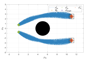
(a) Robust case

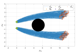
(b) Non-robust case

Figure 1: Two agents scenario with obstacle: Performance comparison between robust and non-robust case with terminal mean and obstacle constraints.

Now, the update steps in an $l^{th}$ iteration of CADMM applied to the problem (54) are as follows.

Local variables update (Block - I)

The update step for the local variables is given by

$$\{\tilde{{\bm{\mu}}}^{\bar{u},l+1}_{i},\;\tilde{{\bm{\mu}}}^{d,l+1}_{i}\}_{i\in\pazocal{V}}$$

$$~{}~{}~{}=\operatornamewithlimits{argmin}\;\pazocal{L}_{\rho_{\bar{u}},\rho_{d}}(\{\tilde{{\bm{\mu}}}^{\bar{u}}_{i},\tilde{{\bm{\mu}}}^{d}_{i},\tilde{{\bm{\nu}}}^{\bar{u},l}_{i},\tilde{{\bm{\nu}}}^{d,l}_{i},{\bm{\lambda}}_{i}^{\bar{u},l},{\bm{\lambda}}_{i}^{d,l}\}_{i\in\pazocal{V}})$$

Note that there is no coupling between the local variables of different agents. Thus, the above update step can be performed in a decentralized manner where each agent $i$ solves its sub-problem to update the local variables $\tilde{{\bm{\mu}}}^{\bar{u},l+1}_{i},\;\tilde{{\bm{\mu}}}^{d,l+1}_{i}$.

Global variables update (Block - II)

Next, the global variables are updated through

$$\{{\bm{\nu}}^{\bar{u},l+1}_{i},\;{\bm{\nu}}^{d,l+1}_{i}\}_{i\in\pazocal{V}}$$

$$~{}~{}~{}=\operatornamewithlimits{argmin}\;\pazocal{L}_{\rho_{\bar{u}},\rho_{d}}(\{\tilde{{\bm{\mu}}}^{\bar{u},l+1}_{i},\tilde{{\bm{\mu}}}^{d,l+1}_{i},\tilde{{\bm{\nu}}}^{\bar{u}}_{i},\tilde{{\bm{\nu}}}^{d}_{i},{\bm{\lambda}}_{i}^{\bar{u},l},{\bm{\lambda}}_{i}^{d,l}\}_{i\in\pazocal{V}})$$

Let us define ${\bm{\lambda}}_{i}^{\bar{u}}$, ${\bm{\lambda}}_{i}^{d}$ as sequence of dual vectors given as ${\bm{\lambda}}_{i}^{\bar{u}}=\begin{bmatrix}\bar{{\bm{\lambda}}}_{i}^{\bar{u}};&\{\bar{{\bm{\lambda}}}_{i}^{j,\bar{u}}\}_{j\in\pazocal{N}_{i}}\end{bmatrix}$, ${\bm{\lambda}}_{i}^{\bar{u}}=\begin{bmatrix}\bar{{\bm{\lambda}}}_{i}^{d};&\{\bar{{\bm{\lambda}}}_{i}^{j,d}\}_{j\in\pazocal{N}_{i}}\end{bmatrix}$, such that the above update can be rewritten in a closed form for each agent $i\in\pazocal{V}$ as follows (details are provided in Section III of the SM)

$${\bm{\nu}}^{\bar{u},l+1}_{i}=\frac{1}{m_{i}}\bigg{(}\frac{\bar{{\bm{\lambda}}}_{i}^{\bar{u},l}}{\rho_{\bar{u}}}+\hat{{\bm{\mu}}}_{i}^{\bar{u},l+1}+\sum_{\hat{j}\in\pazocal{P}_{i}}\big{(}\frac{\bar{{\bm{\lambda}}}_{\hat{j}}^{i,\bar{u},l}}{\rho_{\bar{u}}}+\bar{{\bm{\mu}}}_{\hat{j}}^{i,\bar{u},l+1}\big{)}\bigg{)}$$ (56)

$${\bm{\nu}}^{d,l+1}_{i}=\frac{1}{m_{i}}\bigg{(}\frac{\bar{{\bm{\lambda}}}_{i}^{d,l}}{\rho_{d}}+{\bm{\mu}}^{d,l+1}_{i}+\sum_{\hat{j}\in\pazocal{P}_{i}}\big{(}\frac{\bar{{\bm{\lambda}}}_{\hat{j}}^{i,d,l}}{\rho_{d}}+\bar{{\bm{\mu}}}^{i,d,l+1}_{\hat{j}}\big{)}\bigg{)}$$

where $m_{i}=(n({\pazocal{P}_{i}})+1)$. After the local variables update, each agent $i$ would receive the updated variable $\bar{{\bm{\mu}}}_{\hat{j}}^{i,\bar{u},l+1}$ from all the agents $\hat{j}$ to which it is a neighbor of ($\hat{j}\in\pazocal{P}_{i}$). Using these received local variables, each agent $i$ updates the global variables ${\bm{\nu}}^{\bar{u},l+1}_{i},{\bm{\nu}}^{d,l+1}_{i}$ as per the update step (56).

Dual variables update

Finally, the dual variables are updated through the following rules

$${\bm{\lambda}}_{i}^{\bar{u},l+1}={\bm{\lambda}}_{i}^{\bar{u},l}+\rho_{\bar{u}}(\tilde{{\bm{\mu}}}^{\bar{u},l+1}_{i}-\tilde{{\bm{\nu}}}^{\bar{u},l+1}_{i})$$ (57)

$${\bm{\lambda}}_{i}^{d,l+1}={\bm{\lambda}}_{i}^{d,l}+\rho_{d}(\tilde{{\bm{\mu}}}^{d,l+1}_{i}-\tilde{{\bm{\nu}}}^{d,l+1}_{i})$$

After the global variables update, each agent $i$ would receive the updated global variables ${\bm{\nu}}^{\bar{u},l+1}_{j},{\bm{\nu}}^{d,l+1}_{j}$ from all its neighbor agents $j\in\pazocal{N}_{i}$. Using these received variables, the agent $i$ updates the dual variables ${\bm{\lambda}}_{i}^{\bar{u},l+1},{\bm{\lambda}}_{i}^{d,l+1}$ as per the update step (57). It should be noted that in each update step, all the agents do the update in parallel. Further, the agents need not exchange other system information (such as dynamics parameters or uncertainty set parameters).

IV Simulation Results

In this section, we provide simulation results of the proposed method applied to a multi-agent system with underlying stochastic and deterministic uncertainties. In Section IV-A, the effectiveness of the proposed robust constraints is analyzed under different scenarios. In Section IV-B, the scalability of the proposed distributed framework is illustrated. The agents have 2D double integrator dynamics with the exact dynamic matrices and the uncertainty information provided in Section IV of the SM. In all experiments, we set the time horizon to $T=20$. All experiments are also illustrated through the supplementary video.

IV-A Effectiveness of Proposed Robust Constraints

We start by validating the effectiveness of the proposed robust constraints by considering different cases of underlying uncertainties. First, we analyze the constraints that are only on the expectation of the state. Subsequently, we analyze the robust chance constraints and covariance constraints, which are dependent on both the deterministic and stochastic disturbances.

IV-A1 With deterministic disturbances

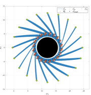
(a) Robust case

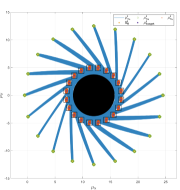
(b) Non-robust case

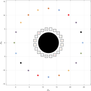
(c) Robust case, $k=0$

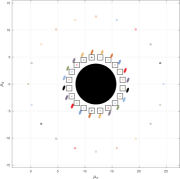
(d) Robust case, $k=10$

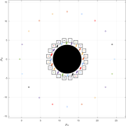
(e) Robust case, $k=15$

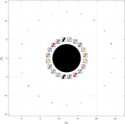
(f) Robust case, $k=20$

Figure 2: Twenty agents scenario with circle formation task and obstacle: (a) with robust constraints, (b) without robust constraints, (c)-(f) Snapshots of mean trajectories of agents in robust case.

Here, we compare the results of applying the proposed distributed framework for two cases: robust and non-robust. With non-robust, we refer to the case of finding the optimal control trajectory by only considering standard optimization constraints instead of explicitly accounting for the deterministic uncertainties through robust optimization constraints (robust case). Fig. 1 discloses a two-agent scenario with terminal mean and obstacle avoidance constraints. The plots demonstrate $100$ trajectories of the two agents for different realizations of the disturbances. As shown in Fig. 1a, in the robust case, each agent $i$ successfully avoids the obstacle, and its disturbance-free state mean reaches the target terminal mean ${\bm{\mu}}_{target}^{i}$ with uncertainty in its terminal state mean lying inside the set target bounds (represented by black boxes). On the contrary, for the non-robust case in Fig. 1b, the agents might collide with the obstacle in the center, and the uncertainty in the terminal state mean of each agent might lie outside the target bounds. In Fig. 2, we present a scenario of 20 agents in a circle formation, where each agent must reach the opposite side while avoiding collisions with other agents and an obstacle in the center. Fig. 2a and 2b show $100$ realizations for the robust and non-robust case. Clearly, the robust approach is able to successfully steer the agents to their targets while avoiding collisions, in contrast with the non-robust case where the agents might collide with the obstacle. In Fig. 2c - 2f, we show snapshots of the robust trajectories of the agents for different time instants, demonstrating that the agents do not violate any of the constraints during the tasks. Further, it is worth noting that in the robust case, the agents not only avoid collision but also the uncertainty in the state mean of an agent is reduced when it approaches an obstacle or another agent.

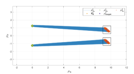
(a)

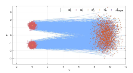
(b)

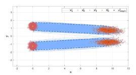
(c)

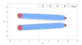
(d)

Figure 3: Performance analysis of robust chance constraints and Covariance Constraints - Scenario 1: (a) Mean trajectories of agents in deterministic case, (b) Trajectories of agents in deterministic case without the robust chance constraints, (c) Trajectories of agents in mixed case with robust chance constraints, (d) Trajectories of agents in mixed case with robust chance constraints and terminal covariance constraints.

IV-A2 With both deterministic and stochastic disturbances

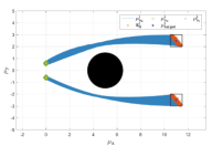
(a)

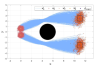
(b)

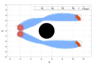
(c)

Figure 4: Performance analysis of robust chance constraints - Scenario 2: (a) Mean trajectories of agents in the deterministic case, (b) Trajectories of agents in the deterministic case without the robust chance constraints, (c) Trajectories of agents in mixed case with robust chance constraints.

In this subsection, we demonstrate the effectiveness of the proposed framework with robust chance constraints and covariance constraints. For that, we compare two cases, one where the constraints that are only on the expectation of the state are active (‘deterministic case’), and another where all the robust constraints, including the robust chance and covariance constraints, are active (‘mixed case’). Further, it should be noted that when both disturbances are present, the mean trajectory differs from the actual trajectory.

We present two scenarios of a two-agent case with different levels of deterministic uncertainty controlled using $\tau_{i}$ but with the same stochastic uncertainty characterized by initial state covariance to be $\mathrm{diag}([0.2,0.2,0.5,0.5])^{2}$, and covariance of each stochastic noise component $w_{i}^{k}$ to be $\mathrm{diag}([0.02,0.02,0.2,0.2])^{2}$ for each agent $i\in\pazocal{V}$. Fig. 3 discloses the first scenario with deterministic uncertainty parameterized by $\tau=0.01$ for both agents. It can be observed from Fig. 3a that the mean trajectories obtained by the proposed method in the deterministic case satisfy the inter-agent and the terminal mean constraints. However, Fig. 3b shows that in the presence of stochastic noise, a collision between the agents is highly probable, and the agents may not be able to reach the targets within the set bounds. Fig. 3c presents the case where we enforce robust chance constraints on the agents’ positions to stay within the blue dashed lines. As shown, most of the realizations of the trajectories lie within the specified bounds of the chance constraints, which ensures the safe operation of the agents despite the stochastic uncertainty. However, the uncertainty in the terminal state of the agents is not controlled by the applied robust chance constraints. We address this using covariance constraints. Fig 3d presents the scenario with additional terminal covariance constraints with the target covariance ${\bm{\Sigma}}^{i}$ set to be $\mathrm{diag}([0.05,0.05,0.5,0.5])^{2}$ for each agent $i\in\pazocal{V}$. It can be observed that the uncertainty in the terminal state is reduced.

Fig. 4 presents the second scenario of the two-agent case that involves a higher deterministic uncertainty parameterized by $\tau=0.05$ for both agents. Fig. 4b shows that the uncertainty in the terminal state of the agents might lie outside the target uncertainty bounds (indicated by black boxes). To address this, we can use covariance steering as shown in the previous scenario, or robust chance constraints. We use robust chance constraints in this scenario. Fig. 4c shows results for the mixed case when robust chance constraints are applied on the terminal state to stay within the target uncertainty bounds represented by the blue dashed box.

Further, it is interesting to note the following two observations. From Fig. 3a and 3d, it should be observed that uncertainty in the state trajectory is reduced to be smaller than the uncertainty in the mean in the deterministic case by adding covariance constraints. From Fig. 4a and 4b, it should be observed that the actual trajectories of the agents in the deterministic case avoid the obstacle without enforcing the robust chance constraints. This is because the feedback control gain ${\bf K}$ is used to control the deviations in the state due to the deterministic and stochastic uncertainties. Thus, controlling the deviation in the state due to one type of uncertainty also controls the deviation due to another. This might be useful in cases where one of the uncertainties (deterministic or stochastic) is significantly higher than the other. In such a case, we need not explicitly apply constraints to control the effect of the least pronounced uncertainty.

IV-B Scalability of Proposed Distributed Framework

In our experiments, we noticed that the centralized method with robust terminal mean and initial approach obstacle avoidance constraints alone would fail for a time horizon longer than 15 and a number of agents greater than 3. Fig. 5 shows the result of the proposed distributed framework applied to a large-scale scenario with 100 agents, which verifies the scalability of the proposed approach. The constraints considered are robust terminal mean and inter-agent constraints. Further, Fig. 6 reports the computational times of the proposed framework for an increasing number of agents for scenarios with robust terminal mean and inter-agent constraints. All simulations were carried out in Matlab2022b [17] environment using CVX [15] as the modeling software and MOSEK as the solver [2] on a system with an Intel Corei9-13900HX.

V Conclusion

In this paper, we merge principles from the areas of robust optimization, distribution steering and distributed optimization towards obtaining a scalable safe multi-agent control method under both stochastic and deterministic uncertainties. In particular, we present a distributed robust optimization method that exploits computationally tractable approximations of robust constraints and the separable nature of ADMM in order to significantly reduce the computational demands that such approaches would typically have when applied to multi-agent systems. The results verify that the proposed framework is able to effectively address both types of uncertainty and scale for multi-robot systems with up to a hundred agents.

In future work, we wish to extend the applicability of the proposed method and explore additional robust optimization formulations that would be relevant for robotics problems. In particular, since the current method considers linear time-varying dynamics, it would be possible to extend for nonlinear systems through sequential linearization schemes [32, 34]. Additionally, we intend to further explore suitable robust optimization formulations for multi-agent robotics and investigate connections with shooting methods [18, 41]. Finally, incorporating the current framework into hierarchical distributed optimization schemes [36] would be a promising direction for further increasing the scalability of the method.

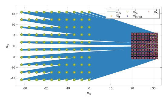
Figure 5: Large-scale scenario with 100 agents: Mean trajectories of the agents with robust terminal mean and inter-agent collision avoidance constraints.

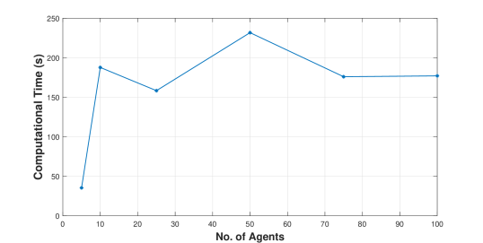
Figure 6: Scalability analysis: Computational times of the proposed distributed framework for an increasing number of agents.

Supplementary Material

In the following, we provide detailed derivations, proofs and experiment data that have been omitted in the main paper.

VI System Dynamics Compact Form

The system dynamics (1) can be written in a more compact form as follows

$${\bm{x}}^{i}={\bf G}_{0}^{i}\bar{x}_{0}^{i}+{\bf G}_{u}^{i}{\bm{u}}^{i}+{\bf G}_{{\bm{w}}}^{i}\bm{{\bm{w}}}^{i}+{\bf G}_{\zeta}^{i}\bm{\zeta}^{i},$$ (58)

where

$${\bf G}_{0}^{i}=\begin{bmatrix}{\bf I};&{\bf\Phi}^{i}(1,0);&{\bf\Phi}^{i}(2,0);&\dots;&{\bf\Phi}^{i}(T,0)\end{bmatrix},$$ (59a)

$${\bf G}_{u}^{i}=\begin{bmatrix}{\bf 0}&{\bf 0}&\dots&{\bf 0}\\ B_{0}^{i}&{\bf 0}&\dots&{\bf 0}\\ {\bf\Phi}^{i}(2,1)B_{0}^{i}&B_{1}^{i}&\dots&{\bf 0}\\ \vdots&\vdots&\vdots&\vdots\\ {\bf\Phi}^{i}(T,1)B_{0}^{i}&{\bf\Phi}^{i}(T,2)B_{1}^{i}&\dots&B_{T-1}^{i}\end{bmatrix},$$ (59b)

$${\bf G}_{{\bm{w}}}^{i}=\begin{bmatrix}{\bf I}&{\bf 0}&\dots&{\bf 0}\\ {\bf\Phi}^{i}(1,0)&D_{0}^{i}&\dots&{\bf 0}\\ {\bf\Phi}^{i}(2,0)&{\bf\Phi}^{i}(2,1)D_{0}^{i}&\dots&{\bf 0}\\ \vdots&\vdots&\vdots&\vdots\\ {\bf\Phi}^{i}(T,0)&{\bf\Phi}^{i}(T,1)D_{0}^{i}&\dots&D_{T-1}^{i}\end{bmatrix},$$ (59c)

$${\bf G}_{\zeta}^{i}=\begin{bmatrix}{\bf I}&{\bf 0}&\dots&{\bf 0}\\ {\bf\Phi}^{i}(1,0)&C_{0}^{i}&\dots&{\bf 0}\\ {\bf\Phi}^{i}(2,0)&{\bf\Phi}^{i}(2,1)C_{0}^{i}&\dots&{\bf 0}\\ \vdots&\vdots&\vdots&\vdots\\ {\bf\Phi}^{i}(T,0)&{\bf\Phi}^{i}(T,1)C_{0}^{i}&\dots&C_{T-1}^{i}\end{bmatrix},$$ (59d)

with

$${\bf\Phi}^{i}(k_{1},k_{2})=A_{k_{1}-1}^{i}A_{k_{1}-2}^{i}\dots A_{k_{2}}^{i}\;\text{for}\;k_{1}>k_{2}.$$ (60)

VII Robust Linear Constraints

VII-A Expectation of State

Let us rewrite the state equation for an agent $i$ as follows

$${\bm{x}}^{i}={\bf G}_{0}^{i}\bar{x}_{0}^{i}+{\bf G}_{u}^{i}{\bm{u}}^{i}+{\bf G}_{{\bm{w}}}^{i}\bm{{\bm{w}}}^{i}+{\bf G}_{\zeta}^{i}\bm{\zeta}^{i}$$

Substituting the control ${\bm{u}}^{i}$ as $\bar{{\bm{u}}}^{i}+{\bf K}^{i}{\bm{\delta}}^{i}$ (from (10)) in the above state equation, we get the following.

$${\bm{x}}^{i}={\bf G}_{0}^{i}\bar{x}_{0}^{i}+{\bf G}_{u}^{i}\big{(}\bar{{\bm{u}}}^{i}+{\bf K}^{i}{\bm{\delta}}^{i}\big{)}+{\bf G}_{{\bm{w}}}^{i}\bm{{\bm{w}}}^{i}+{\bf G}_{\zeta}^{i}\bm{\zeta}^{i}$$ (61)

Further, using (8), we can rewrite the above equation as follows

$${\bm{x}}^{i} ={\bf G}_{0}^{i}\bar{x}_{0}^{i}+{\bf G}_{u}^{i}\big{(}\bar{{\bm{u}}}^{i}+{\bf K}^{i}({\bf G}_{{\bm{w}}}^{i}\bm{{\bm{w}}}^{i}+{\bf G}_{\zeta}^{i}\bm{\zeta}^{i})\big{)}$$ (62)

$$~{}~{}+{\bf G}_{{\bm{w}}}^{i}\bm{{\bm{w}}}^{i}+{\bf G}_{\zeta}^{i}\bm{\zeta}^{i}$$

which can be written in compact form as follows -

$${\bm{x}}^{i} ={\bf G}_{0}^{i}\bar{x}_{0}^{i}+{\bf G}_{u}^{i}\bar{{\bm{u}}}^{i}+({\bf G}_{u}^{i}{\bf K}^{i}+{\bf I}){\bf G}_{{\bm{w}}}^{i}\bm{{\bm{w}}}^{i}$$ (63)

$$~{}~{}~{}+({\bf G}_{u}^{i}{\bf K}^{i}+{\bf I}){\bf G}_{\zeta}^{i}\bm{\zeta}^{i}$$

Now, the expectation of the state can be given as

$$E[{\bm{x}}^{i}] ={\bf G}_{0}^{i}\bar{x}_{0}^{i}+{\bf G}_{u}^{i}\bar{{\bm{u}}}^{i}+({\bf G}_{u}^{i}{\bf K}^{i}+{\bf I}){\bf G}_{{\bm{w}}}^{i}E[\bm{{\bm{w}}}^{i}]$$ (64)

$$~{}~{}~{}+({\bf G}_{u}^{i}{\bf K}^{i}+{\bf I}){\bf G}_{\zeta}^{i}\bm{\zeta}^{i}$$

Finally, using the fact that $E[\bm{{\bm{w}}}^{i}]=0$, we get

$$E[{\bm{x}}^{i}]={\bf G}_{0}^{i}\bar{x}_{0}^{i}+{\bf G}_{u}^{i}\bar{{\bm{u}}}^{i}+({\bf G}_{u}^{i}{\bf K}^{i}+{\bf I}){\bf G}_{\zeta}^{i}\bm{\zeta}^{i}$$ (65)

VII-B Covariance of State

The covariance of the state of an agent $i$ is given as follows

$$\mathrm{Cov}[{\bm{x}}^{i}]=\mathbb{E}\Big{[}({\bm{x}}^{i}-\mathbb{E}[{\bm{x}}^{i}])({\bm{x}}^{i}-\mathbb{E}[{\bm{x}}^{i}])^{\mathrm{T}}\Big{]}$$ (66)

Let us first write the expression for ${\bm{x}}^{i}-\mathbb{E}[{\bm{x}}^{i}]$ using (63) and (65) as follows

$${\bm{x}}^{i}-\mathbb{E}[{\bm{x}}^{i}]=({\bf G}_{u}^{i}{\bf K}^{i}+{\bf I}){\bf G}_{{\bm{w}}}^{i}\bm{{\bm{w}}}^{i}$$ (67)

Now, the covariance of the state can be rewritten as -

$$\mathrm{Cov}[{\bm{x}}^{i}]=\mathbb{E}\Big{[}({\bf G}_{u}^{i}{\bf K}^{i}+{\bf I}){\bf G}_{{\bm{w}}}^{i}\bm{{\bm{w}}}^{i}(({\bf G}_{u}^{i}{\bf K}^{i}+{\bf I}){\bf G}_{{\bm{w}}}^{i}\bm{{\bm{w}}}^{i})^{\mathrm{T}}\Big{]}$$ (68)

which can be further rewritten as

$$\mathrm{Cov}[{\bm{x}}^{i}]=({\bf G}_{u}^{i}{\bf K}^{i}+{\bf I}){\bf G}_{{\bm{w}}}^{i}\mathbb{E}[\bm{{\bm{w}}}^{i}\bm{{\bm{w}}}^{i}{}^{\mathrm{T}}]{\bf G}_{{\bm{w}}}^{i}{}^{\mathrm{T}}({\bf G}_{u}^{i}{\bf K}^{i}+{\bf I})^{\mathrm{T}}$$ (69)

Finally, using the fact that $\mathbb{E}[\bm{{\bm{w}}}^{i}\bm{{\bm{w}}}^{i}{}^{\mathrm{T}}]={\bm{\Sigma}}_{{\bm{w}}^{i}}$, we get

$$\mathrm{Cov}[{\bm{x}}^{i}]=({\bf G}_{u}^{i}{\bf K}^{i}+{\bf I}){\bf G}_{{\bm{w}}}^{i}{\bm{\Sigma}}_{{\bm{w}}^{i}}{\bf G}_{{\bm{w}}}^{i}{}^{\mathrm{T}}({\bf G}_{u}^{i}{\bf K}^{i}+{\bf I})^{\mathrm{T}}$$ (70)

VII-C Proposition 1 Proof

The expression $\max_{{\bm{\zeta}}^{i}\in\pazocal{U}_{i}}{\bm{a}}_{i}^{\mathrm{T}}\mathbb{E}[{\bm{x}}^{i}]$ can be rewritten as

$$\max_{{\bm{\zeta}}^{i}\in\pazocal{U}_{i}}{\bm{a}}_{i}^{\mathrm{T}}\mathbb{E}[{\bm{x}}^{i}] ={\bm{a}}_{i}^{\mathrm{T}}{\bm{\mu}}_{x,\bar{u}}^{i}+\max_{{\bm{\zeta}}^{i}\in\pazocal{U}_{i}}{\bm{a}}_{i}^{\mathrm{T}}{\bf M}_{i}{\bm{\zeta}}^{i}$$ (71a)

$$={\bm{a}}_{i}^{\mathrm{T}}{\bm{\mu}}_{x,\bar{u}}^{i}-\min_{\langle{\bf S}_{i}{\bm{z}}_{i},{\bm{z}}_{i}\rangle\leq\tau^{i}}-{\bm{a}}_{i}^{\mathrm{T}}{\bf M}_{i}\bm{\Gamma}_{i}{\bm{z}}_{i}.$$ (71b)

Let us now consider the Lagrangian for the minimization problem inside (71b), given by

$$\pazocal{L}({\bm{z}}_{i},\lambda)=-{\bm{a}}_{i}^{\mathrm{T}}{\bf M}_{i}\bm{\Gamma}_{i}{\bm{z}}_{i}+\lambda(\langle{\bf S}_{i}{\bm{z}}_{i},{\bm{z}}_{i}\rangle-\tau^{i}),$$ (72)

where $\lambda\in\mathbb{R}$ is the Lagrange multiplier corresponding to the inequality constraint $\langle{\bf S}_{i}{\bm{z}}_{i},{\bm{z}}_{i}\rangle\leq\tau^{i}$. The above problem is convex, and the constraint set $\langle{\bf S}_{i}{\bm{z}}_{i},{\bm{z}}_{i}\rangle\leq\tau^{i}$ is non-empty - since ${\bm{z}}_{i}=0$ lies in the interior of the feasible set because $\tau^{i}>0$. Thus, the problem satisfies Slater’s condition, and we could find the minimizer using KKT conditions as follows

$$\nabla_{{\bm{z}}_{i}}\pazocal{L}({\bm{z}}_{i}^{*},\lambda^{*})=0,$$ (73a)

$$\lambda^{*}(\langle{\bf S}_{i}{\bm{z}}_{i}^{*},{\bm{z}}_{i}^{*}\rangle-\tau^{i})=0,$$ (73b)

$$\lambda^{*}\geq 0,$$ (73c)

$$\langle{\bf S}_{i}{\bm{z}}_{i}^{*},{\bm{z}}_{i}^{*}\rangle-\tau^{i}\leq 0.$$ (73d)

Let us first simplify the condition $\nabla_{{\bm{z}}_{i}}\pazocal{L}({\bm{z}}_{i}^{*},\lambda^{*})=0$, as

$$-\bm{\Gamma}_{i}^{\mathrm{T}}{\bf M}_{i}^{\mathrm{T}}{\bm{a}}_{i}+2\lambda^{*}{\bf S}_{i}{\bm{z}}_{i}^{*}=0,$$ (74)

which leads to

$$2\lambda^{*}{\bm{z}}_{i}^{*}={\bf S}_{i}^{-1}\bm{\Gamma}_{i}^{\mathrm{T}}{\bf M}_{i}^{\mathrm{T}}{\bm{a}}_{i}.$$ (75)

It can be observed that $\bm{\Gamma}_{i}^{\mathrm{T}}{\bf M}_{i}^{\mathrm{T}}{\bm{a}}_{i}$ cannot be equal to the zero vector since it is the coefficient of ${\bm{z}}_{i}$ in the objective function. Thus, since we also have that ${\bf S}_{i}\in\mathbb{S}_{++}^{\bar{n}_{i}}$, then the RHS of the above equation is non-zero, which implies that both ${\bm{z}}_{i}^{*}$ and $\lambda^{*}$ need to be non-zero. Therefore, we obtain

$${\bm{z}}_{i}^{*}=(2\lambda^{*})^{-1}{\bf S}_{i}^{-1}\bm{\Gamma}_{i}^{\mathrm{T}}{\bf M}_{i}^{\mathrm{T}}{\bm{a}}_{i}.$$ (76)

Further, from the condition (73b) and using $\lambda^{*}\neq 0$, we get

$$\langle{\bf S}_{i}{\bm{z}}_{i}^{*},{\bm{z}}_{i}^{*}\rangle-\tau^{i}=0,$$ (77)

which through (76) gives

$$(2\lambda^{*})^{-2}\langle\bm{\Gamma}_{i}^{\mathrm{T}}{\bf M}_{i}^{\mathrm{T}}{\bm{a}}_{i},\;{\bf S}_{i}^{-1}\bm{\Gamma}_{i}^{\mathrm{T}}{\bf M}_{i}^{\mathrm{T}}{\bm{a}}_{i}\rangle=\tau^{i},$$ (78)

The above relationship leads to

$$(\tau^{i})^{-1/2}\;\|\bm{\Gamma}_{i}^{\mathrm{T}}{\bf M}_{i}^{\mathrm{T}}{\bm{a}}_{i}\|_{{\bf S}_{i}^{-1}}=2\lambda^{*},$$ (79)

since $\lambda^{*}>0$. The optimal value $\pazocal{L}({\bm{z}}_{i}^{*},\lambda^{*})$ is then given by

$$\pazocal{L}({\bm{z}}_{i}^{*},\lambda^{*}) =-{\bm{a}}_{i}^{\mathrm{T}}{\bf M}_{i}\bm{\Gamma}_{i}{\bm{z}}_{i}^{*}$$ (80a)

$$=-(2\lambda^{*})^{-1}{\bm{a}}_{i}^{\mathrm{T}}{\bf M}_{i}\bm{\Gamma}_{i}{\bf S}_{i}^{-1}\bm{\Gamma}_{i}^{\mathrm{T}}{\bf M}_{i}^{\mathrm{T}}{\bm{a}}_{i}$$ (80b)

$$=-(2\lambda^{*})^{-1}\|\bm{\Gamma}_{i}^{\mathrm{T}}{\bf M}_{i}^{\mathrm{T}}{\bm{a}}_{i}\|_{{\bf S}_{i}^{-1}}^{2}$$ (80c)

$$=-(\tau^{i})^{1/2}\|\bm{\Gamma}_{i}^{\mathrm{T}}{\bf M}_{i}^{\mathrm{T}}{\bm{a}}_{i}\|_{{\bf S}_{i}^{-1}}.$$ (80d)

Therefore, we obtain

$$\max_{{\bm{\zeta}}^{i}\in\pazocal{U}_{i}}{\bm{a}}_{i}^{\mathrm{T}}\mathbb{E}[{\bm{x}}^{i}] ={\bm{a}}_{i}^{\mathrm{T}}{\bm{\mu}}_{x,\bar{u}}^{i}-\pazocal{L}({\bm{z}}_{i}^{*},\lambda^{*})$$ (81a)

$$={\bm{a}}_{i}^{\mathrm{T}}{\bm{\mu}}_{x,\bar{u}}^{i}+(\tau^{i})^{1/2}\|\bm{\Gamma}_{i}^{\mathrm{T}}{\bf M}_{i}^{\mathrm{T}}{\bm{a}}_{i}\|_{{\bf S}_{i}^{-1}}.$$ (81b)

VIII Robust Non-convex Constraints and Distributed Architecture

VIII-A Initial Approach for robust nonconvex constraint

Let us rewrite the robust nonconvex norm-of-mean constraint (26) as follows

$$\min_{{\bm{\zeta}}^{i}\in\pazocal{U}_{i}}\|{\bf A}_{i}{\bf P}_{k}^{i}{\bm{\mu}}_{x,\bar{u}}^{i}+{\bf A}_{i}{\bf P}^{i}_{k}{\bf M}_{i}{\bm{\zeta}}^{i}-\bm{b}_{i}\|_{2}\geq c_{i},$$ (82)

which can be written in terms of ${\bm{\zeta}}^{i}$ as

$$\min_{{\bm{\zeta}}^{i}\in\pazocal{U}_{i}}{\bm{\zeta}}^{i}{}^{\mathrm{T}}{\bf F}_{1,k}^{i}({\bf K}^{i}){\bm{\zeta}}^{i}+2{\bf F}_{2,k}^{i}({\bf K}^{i}, \bar{{\bm{u}}}^{i}){\bm{\zeta}}^{i}$$ (83)

$$+{\bf F}_{3,k}^{i}(\bar{{\bm{u}}}^{i})\geq c_{i}^{2}$$

where

$${\bf F}_{1,k}^{i}({\bf K}^{i}) =({\bf A}_{i}{\bf P}^{i}_{k}{\bf M}_{i})^{\mathrm{T}}{\bf A}_{i}{\bf P}^{i}_{k}{\bf M}_{i},$$ (84a)

$${\bf F}_{2,k}^{i}({\bf K}^{i},\bar{{\bm{u}}}^{i}) =({\bf A}_{i}{\bf P}_{k}^{i}{\bm{\mu}}_{x,\bar{u}}^{i}-\bm{b}_{i})^{\mathrm{T}}({\bf A}_{i}{\bf P}^{i}_{k}{\bf M}_{i}),$$ (84b)

$${\bf F}_{3,k}^{i}(\bar{{\bm{u}}}^{i}) =\|{\bf A}_{i}{\bf P}_{k}^{i}{\bm{\mu}}_{x,\bar{u}}^{i}-\bm{b}_{i}\|_{2}^{2}.$$ (84c)

The constraint (83) could be reformulated through the following equivalent set of constraints (see [19]),

$$\begin{bmatrix}\bm{\Gamma}_{i}^{\mathrm{T}}{\bf F}_{1,k}^{i}({\bf K}^{i})\bm{\Gamma}_{i}+\alpha{\bf S}_{i}&\bm{\Gamma}_{i}^{\mathrm{T}}{\bf F}_{2,k}^{i}({\bf K}^{i},\bar{u}^{i})^{\mathrm{T}}\\ {\bf F}_{2,k}^{i}({\bf K}^{i},\bar{u}^{i})\bm{\Gamma}_{i}&{\bf F}_{3,k}^{i}(\bar{u}^{i})-c_{i}^{2}-\alpha\tau^{i}\end{bmatrix}\succeq 0,$$ (85a)

$$~{}~{}~{}~{}~{}~{}~{}~{}~{}~{}~{}~{}~{}~{}~{}~{}~{}~{}~{}~{}~{}~{}~{}~{}~{}~{}~{}\alpha\geq 0.$$ (85b)

Nevertheless, the above constraint would still be a nonconvex constraint, as ${\bf F}_{1,k}^{i}({\bf K}^{i})$, ${\bf F}_{2,k}^{i}({\bf K}^{i},\bar{u}^{i})$, and ${\bf F}_{3,k}^{i}(\bar{u}^{i})$ are nonlinear in ${\bf K}^{i}$, $\bar{u}^{i}$. To address this issue, we first linearize the constraint (82) with respect to ${\bf K}^{i},\bar{u}^{i}$ around the nominal ${\bf K}^{i,l},\bar{u}^{i,l}$, to obtain the following affine robust constraint

$$\bm{\zeta}^{i}{}^{\mathrm{T}}\mathscr{Q}({\bf K}^{i},{\bf K}^{i,l})\bm{\zeta}^{i}+2 \bar{\mathscr{Q}}({\bf K}^{i},{\bf K}^{i,l},\bar{{\bm{u}}}^{i},\bar{{\bm{u}}}^{i,l})\bm{\zeta}^{i}$$ (86)

$$+q(\bar{{\bm{u}}}^{i},\bar{{\bm{u}}}^{i,l})\geq c_{i}^{2},\quad\forall\;\bm{\zeta}^{i}\in\pazocal{U}_{i}$$

where

$$\mathscr{Q}=({\bf A}_{i}{\bf P}^{i}_{k}{\bf M}_{i}^{l})^{\mathrm{T}}{\bf A}_{i}{\bf P}^{i}_{k}{\bf M}_{i}$$

$$~{}~{}~{}~{}~{}~{}~{}~{}~{}~{}~{}~{}~{}~{}~{}~{}~{}+({\bf A}_{i}{\bf P}^{i}_{k}({\bf M}_{i}-{\bf M}_{i}^{l}))^{\mathrm{T}}{\bf A}_{i}{\bf P}^{i}_{k}{\bf M}_{i}^{l},$$ (87a)

$$\bar{\mathscr{Q}}=({\bf A}_{i}{\bf P}_{k}^{i}{\bm{\mu}}_{x,\bar{u}}^{i,l}-\bm{b}_{i})^{\mathrm{T}}({\bf A}_{i}{\bf P}^{i}_{k}{\bf M}_{i})$$

$$~{}~{}~{}~{}~{}~{}~{}~{}~{}~{}~{}~{}~{}~{}~{}~{}~{}+({\bf A}_{i}{\bf P}_{k}^{i}({\bm{\mu}}_{x,\bar{u}}^{i}-{\bm{\mu}}_{x,\bar{u}}^{i,l}))^{\mathrm{T}}({\bf A}_{i}{\bf P}^{i}_{k}{\bf M}_{i}^{l}),$$ (87b)

$$q=({\bf A}_{i}{\bf P}_{k}^{i}{\bm{\mu}}_{x,\bar{u}}^{i,l}-\bm{b}_{i})^{\mathrm{T}}({\bf A}_{i}{\bf P}_{k}^{i}(2{\bm{\mu}}_{x,\bar{u}}^{i}-{\bm{\mu}}_{x,\bar{u}}^{i,l})-\bm{b}_{i}).$$ (87c)

VIII-B Proposition 2 Proof

Let us initially rewrite the constraint (33) as follows

$$\max_{{\bm{\zeta}}^{i}\in\pazocal{U}_{i}}\|{\bf A}_{i}\tilde{{\bf M}}_{k}^{i}{\bm{\zeta}}^{i}\|_{2}\leq\tilde{c}_{i}-c_{i}.$$ (88)

The first step is to construct an upper bound for $\|{\bf A}_{i}\tilde{{\bf M}}_{k}^{i}{\bm{\zeta}}^{i}\|_{2}^{2}$. Using Proposition 1, we obtain the following two equalities,

$$\max_{{\bm{\zeta}}^{i}\in\pazocal{U}_{i}}h_{k,\bar{m}}^{i}{}^{\mathrm{T}}{\bf M}_{i}{\bm{\zeta}}^{i} =(\tau^{i})^{1/2}\|\bm{\Gamma}_{i}^{\mathrm{T}}{\bf M}_{i}^{\mathrm{T}}h_{k,\bar{m}}^{i}\|_{{\bf S}_{i}^{-1}},$$ (89)

$$\min_{{\bm{\zeta}}^{i}\in\pazocal{U}_{i}}h_{k,\bar{m}}^{i}{}^{\mathrm{T}}{\bf M}_{i}{\bm{\zeta}}^{i} =-(\tau^{i})^{1/2}\|\bm{\Gamma}_{i}^{\mathrm{T}}{\bf M}_{i}^{\mathrm{T}}h_{k,\bar{m}}^{i}\|_{{\bf S}_{i}^{-1}},$$ (90)

where $h_{k,\bar{m}}^{i}{}^{\mathrm{T}}$ is $\bar{m}^{th}$ row of ${\bf A}_{i}{\bf P}_{k}^{i}$, for all $\bar{m}=1,\dots,m$. By combining (89) and (90) for every row of ${\bf A}_{i}\tilde{{\bf M}}_{k}^{i}{\bm{\zeta}}^{i}$, we can arrive to the following relationship,

$$\max_{{\bm{\zeta}}^{i}\in\pazocal{U}_{i}}\|{\bf A}_{i}\tilde{{\bf M}}_{k}^{i}{\bm{\zeta}}^{i}\|_{2} =\max_{{\bm{\zeta}}^{i}\in\pazocal{U}_{i}}\bigg{(}\sum_{\bar{m}=1}^{m}(h_{k,\bar{m}}^{i}{}^{\mathrm{T}}{\bf M}_{i}{\bm{\zeta}}^{i})^{2}\bigg{)}^{1/2}$$ (91a)

$$\leq\bigg{(}\sum_{\bar{m}=1}^{m}\max_{{\bm{\zeta}}^{i}\in\pazocal{U}_{i}}(h_{k,\bar{m}}^{i}{}^{\mathrm{T}}{\bf M}_{i}{\bm{\zeta}}^{i})^{2}\bigg{)}^{1/2}$$ (91b)

$$~{}~{}=\bigg{(}\sum_{\bar{m}=1}^{m}\tau^{i}\|\bm{\Gamma}_{i}^{\mathrm{T}}{\bf M}_{i}^{\mathrm{T}}h_{k,\bar{m}}^{i}\|_{{\bf S}_{i}^{-1}}^{2}\bigg{)}^{1/2}$$ (91c)

Next, by introducing a variable ${\bm{\mu}}_{d,k}^{i}$ such that

$$(\tau^{i})^{1/2}\|\bm{\Gamma}_{i}^{\mathrm{T}}{\bf M}_{i}^{\mathrm{T}}h_{k,\bar{m}}^{i}\|_{{\bf S}_{i}^{-1}}\leq({\bm{\mu}}_{d,k}^{i})_{\bar{m}},$$ (92)

for every $\bar{m}=1,\dots,m$, we obtain

$$\max_{{\bm{\zeta}}^{i}\in\pazocal{U}_{i}}\|{\bf A}_{i}\tilde{{\bf M}}_{k}^{i}{\bm{\zeta}}^{i}\|_{2}\leq\|{\bm{\mu}}_{d,k}^{i}{}\|_{2}.$$ (93)

Therefore, we can consider the following tighter approximation of the constraint (88), given by

$$\|{\bm{\mu}}_{d,k}^{i}{}\|_{2}\leq\tilde{c}_{i}-c_{i}.$$ (94)

VIII-C Proposition 3 Proof

The proof of Proposition 3 is similar to the one of Proposition 2. First, let us rewrite constraint (40) as follows

$$\max_{{\bm{\zeta}}^{i}\in\pazocal{U}_{i},~{}{\bm{\zeta}}^{j}\in\pazocal{U}_{j}}\|{\bf A}_{i}\tilde{{\bf M}}_{k}^{i}{\bm{\zeta}}^{i}-{\bf A}_{j}\tilde{{\bf M}}_{k}^{j}{\bm{\zeta}}^{j}\|_{2}\leq\tilde{c}_{ij}-c_{ij}.$$ (95)

The bound on each $\bar{m}^{th}$ row of ${\bf A}_{i}\tilde{{\bf M}}_{k}^{i}{\bm{\zeta}}^{i}-{\bf A}_{j}\tilde{{\bf M}}_{k}^{j}{\bm{\zeta}}^{j}$, with $\bar{m}=1,\dots,m$, can be given as follows

$$\max_{{\bm{\zeta}}^{i}\in\pazocal{U}_{i},~{}{\bm{\zeta}}^{j}\in\pazocal{U}_{j}}({\bf A}_{i}\tilde{{\bf M}}_{k}^{i}{\bm{\zeta}}^{i}-{\bf A}_{j}\tilde{{\bf M}}_{k}^{j}{\bm{\zeta}}^{j})_{\bar{m}}={\bm{\mu}}_{max,\bar{m}}^{i}-{\bm{\mu}}_{min,\bar{m}}^{j}$$ (96a)

$$\min_{{\bm{\zeta}}^{i}\in\pazocal{U}_{i},~{}{\bm{\zeta}}^{j}\in\pazocal{U}_{j}}({\bf A}_{i}\tilde{{\bf M}}_{k}^{i}{\bm{\zeta}}^{i}-{\bf A}_{j}\tilde{{\bf M}}_{k}^{j}{\bm{\zeta}}^{j})_{\bar{m}}={\bm{\mu}}_{min,\bar{m}}^{i}-{\bm{\mu}}_{max,\bar{m}}^{j}$$ (96b)

where

$${\bm{\mu}}_{min,\bar{m}}^{i} =\min_{{\bm{\zeta}}^{i}\in\pazocal{U}_{i}}({\bf A}_{i}\tilde{{\bf M}}_{k}^{i}{\bm{\zeta}}^{i})_{\bar{m}},$$ (97)

$${\bm{\mu}}_{max,\bar{m}}^{i} =\max_{{\bm{\zeta}}^{i}\in\pazocal{U}_{i}}({\bf A}_{i}\tilde{{\bf M}}_{k}^{i}{\bm{\zeta}}^{i})_{\bar{m}},$$

$${\bm{\mu}}_{min,\bar{m}}^{j} =\min_{{\bm{\zeta}}^{j}\in\pazocal{U}_{j}}({\bf A}_{j}\tilde{{\bf M}}_{k}^{j}{\bm{\zeta}}^{j})_{\bar{m}},$$

$${\bm{\mu}}_{max,\bar{m}}^{j} =\max_{{\bm{\zeta}}^{j}\in\pazocal{U}_{j}}({\bf A}_{j}\tilde{{\bf M}}_{k}^{j}{\bm{\zeta}}^{j})_{\bar{m}}.$$

Using Proposition 1, we have

$${\bm{\mu}}_{max,\bar{m}}^{i}=-{\bm{\mu}}_{min,\bar{m}}^{i}=(\tau^{i})^{1/2}\|\bm{\Gamma}_{i}^{\mathrm{T}}{\bf M}_{i}^{\mathrm{T}}h_{k,\bar{m}}^{i}\|_{{\bf S}_{i}^{-1}}$$ (98a)

$${\bm{\mu}}_{max,\bar{m}}^{j}=-{\bm{\mu}}_{min,\bar{m}}^{j}=(\tau^{j})^{1/2}\|\bm{\Gamma}_{j}^{\mathrm{T}}{\bf M}_{j}^{\mathrm{T}}h_{k,\bar{m}}^{j}\|_{{\bf S}_{j}^{-1}}$$ (98b)

where $h_{k,\bar{m}}^{i}{}^{\mathrm{T}},h_{k,\bar{m}}^{j}{}^{\mathrm{T}}$ are the $\bar{m}^{th}$ rows of the matrices ${\bf A}_{i}{\bf P}_{k}^{i},{\bf A}_{j}{\bf P}_{k}^{j}$ respectively. By combining (96) and (98), we obtain

$$\max_{{\bm{\zeta}}^{i}\in\pazocal{U}_{i},~{}{\bm{\zeta}}^{j}\in\pazocal{U}_{j}}\|{\bf A}_{i}\tilde{{\bf M}}_{k}^{i}{\bm{\zeta}}^{i}-{\bf A}_{j}\tilde{{\bf M}}_{k}^{j}{\bm{\zeta}}^{j}\|_{2}$$ (99)

$$\qquad\leq\bigg{(}\sum_{\bar{m}=1}^{m}\max_{{\bm{\zeta}}^{i}\in\pazocal{U}_{i},~{}{\bm{\zeta}}^{j}\in\pazocal{U}_{j}}({\bf A}_{i}\tilde{{\bf M}}_{k}^{i}{\bm{\zeta}}^{i}-{\bf A}_{j}\tilde{{\bf M}}_{k}^{j}{\bm{\zeta}}^{j})_{\bar{m}}^{2}\bigg{)}^{1/2}$$

$$~{}\qquad=\bigg{(}\sum_{\bar{m}=1}^{m}({\bm{\mu}}_{max,\bar{m}}^{i}+{\bm{\mu}}_{max,\bar{m}}^{j})^{2}\bigg{)}^{1/2}$$

As in the proof of Proposition 2, let us now introduce the variables ${\bm{\mu}}_{d,k}^{i},{\bm{\mu}}_{d,k}^{j}$ such that

$$({\bm{\mu}}_{d,k}^{i})_{\bar{m}}\geq(\tau^{i})^{1/2}\|\bm{\Gamma}_{i}^{\mathrm{T}}{\bf M}_{i}^{\mathrm{T}}h_{k,\bar{m}}^{i}\|_{{\bf S}_{i}^{-1}}$$ (100)

$$({\bm{\mu}}_{d,k}^{j})_{\bar{m}}\geq(\tau^{j})^{1/2}\|\bm{\Gamma}_{j}^{\mathrm{T}}{\bf M}_{j}^{\mathrm{T}}h_{k,\bar{m}}^{j}\|_{{\bf S}_{j}^{-1}}$$ (101)

for every $\bar{m}=1,\dots,m$. Then, we obtain

$$\max_{{\bm{\zeta}}^{i}\in\pazocal{U}_{i},~{}{\bm{\zeta}}^{j}\in\pazocal{U}_{j}}\|{\bf A}_{i}\tilde{{\bf M}}_{k}^{i}{\bm{\zeta}}^{i} -{\bf A}_{j}\tilde{{\bf M}}_{k}^{j}{\bm{\zeta}}^{j}\|_{2}\leq\|{\bm{\mu}}_{d,k}^{i}+{\bm{\mu}}_{d,k}^{j}\|_{2}$$ (102)

so we can consider the following tighter approximation to the constraint (95),

$$\|{\bm{\mu}}_{d,k}^{i}+{\bm{\mu}}_{d,k}^{j}\|_{2}\leq\tilde{c}_{ij}-c_{ij}.$$ (103)

VIII-D Distributed Architecture Global Updates

The global update steps are given by

$$\{{\bm{\nu}}^{\bar{u},l+1}_{i},\;{\bm{\nu}}^{d,l+1}_{i}\}_{i=1}^{N}$$

$$~{}~{}~{}=\operatornamewithlimits{argmin}\;\pazocal{L}_{\rho_{\bar{u}},\rho_{d}}(\{\tilde{{\bm{\mu}}}^{\bar{u},l+1}_{i},\tilde{{\bm{\mu}}}^{d,l+1}_{i},\tilde{{\bm{\nu}}}^{\bar{u}}_{i},\tilde{{\bm{\nu}}}^{d}_{i},{\bm{\lambda}}_{i}^{\bar{u},l},{\bm{\lambda}}_{i}^{d,l}\}_{i=1}^{N})$$

$$~{}~{}~{}=\operatornamewithlimits{argmin}\;\sum_{i=1}^{N}{\bm{\lambda}}_{i}^{\bar{u}}{}^{\mathrm{T}}(\tilde{{\bm{\mu}}}^{\bar{u}}_{i}-\tilde{{\bm{\nu}}}^{\bar{u}}_{i})+{\bm{\lambda}}_{i}^{d}{}^{\mathrm{T}}(\tilde{{\bm{\mu}}}^{d}_{i}-\tilde{{\bm{\nu}}}^{d}_{i})$$ (104)

$$~{}~{}~{}~{}\qquad\qquad+\frac{\rho_{\bar{u}}}{2}\|\tilde{{\bm{\mu}}}^{\bar{u}}_{i}-\tilde{{\bm{\nu}}}^{\bar{u}}_{i}\|_{2}^{2}+\frac{\rho_{d}}{2}\|\tilde{{\bm{\mu}}}^{d}_{i}-\tilde{{\bm{\nu}}}^{d}_{i}\|_{2}^{2}$$

This update can be decoupled for each agent $i$ as follows

$${\bm{\nu}}^{\bar{u},l+1}_{i},{\bm{\nu}}^{d,l+1}_{i}$$ (105)

$$~{}~{}~{}=\operatornamewithlimits{argmin}_{{\bm{\nu}}^{\bar{u}}_{i},{\bm{\nu}}^{d}_{i}}\;\bar{{\bm{\lambda}}}_{i}^{\bar{u},l}{}^{\mathrm{T}}(\hat{{\bm{\mu}}}^{\bar{u},l+1}_{i}-{\bm{\nu}}^{\bar{u}}_{i})+\bar{{\bm{\lambda}}}_{i}^{d,l}{}^{\mathrm{T}}({\bm{\mu}}^{d,l+1}_{i}-{\bm{\nu}}^{d}_{i})$$

$$~{}~{}~{}\qquad\qquad+\frac{\rho_{\bar{u}}}{2}\|\hat{{\bm{\mu}}}^{\bar{u},l+1}_{i}-{\bm{\nu}}^{\bar{u}}_{i}\|_{2}^{2}+\frac{\rho_{d}}{2}\|{\bm{\mu}}^{d,l+1}_{i}-{\bm{\nu}}^{d}_{i}\|_{2}^{2}$$

$$~{}~{}~{}\qquad\qquad+\sum_{\hat{j}\in\pazocal{P}_{i}}\big{(}\bar{{\bm{\lambda}}}_{\hat{j}}^{i,\bar{u},l}{}^{\mathrm{T}}(\bar{{\bm{\mu}}}^{i,\bar{u},l+1}_{\hat{j}}-{\bm{\nu}}^{\bar{u}}_{i})$$

$$~{}~{}~{}\qquad\qquad+\bar{{\bm{\lambda}}}_{\hat{j}}^{i,d,l}{}^{\mathrm{T}}(\bar{{\bm{\mu}}}^{i,d,l+1}_{\hat{j}}-{\bm{\nu}}^{d}_{i})+\frac{\rho_{\bar{u}}}{2}\|\bar{{\bm{\mu}}}^{i,\bar{u},l+1}_{\hat{j}}-{\bm{\nu}}^{\bar{u}}_{i}\|_{2}^{2}$$

$$~{}~{}~{}\qquad\qquad+\frac{\rho_{d}}{2}\|\bar{{\bm{\mu}}}^{i,d,l+1}_{\hat{j}}-{\bm{\nu}}^{d}_{i}\|_{2}^{2}\big{)}$$

To find the minimum on the RHS, let us differentiate the RHS with respect to the global variables ${\bm{\nu}}^{\bar{u}}_{i},{\bm{\nu}}^{d}_{i}$ and equate it to zero. For ${\bm{\nu}}^{\bar{u},l+1}_{i}$, we get

$$-\bar{{\bm{\lambda}}}_{i}^{\bar{u},l}+\rho_{\bar{u}}(\hat{{\bm{\mu}}}^{\bar{u},l+1}_{i}-{\bm{\nu}}^{\bar{u}}_{i})$$ (106)

$$\qquad+\sum_{\hat{j}\in\pazocal{P}_{i}}\big{(}-\bar{{\bm{\lambda}}}_{\hat{j}}^{i,\bar{u},l}+\rho_{\bar{u}}(\bar{{\bm{\mu}}}^{i,\bar{u},l+1}_{\hat{j}}-{\bm{\nu}}^{\bar{u}}_{i})\big{)}=0$$

which leads to

$${\bm{\nu}}^{\bar{u},l+1}_{i} =\frac{1}{(n(\pazocal{P}_{i})+1)}\bigg{(}\frac{\bar{{\bm{\lambda}}}_{i}^{\bar{u},l}}{\rho_{\bar{u}}}+\hat{{\bm{\mu}}}_{i}^{\bar{u},l+1}$$ (107)

$$\qquad\qquad+\sum_{\hat{j}\in\pazocal{P}_{i}}\big{(}\frac{\bar{{\bm{\lambda}}}_{\hat{j}}^{i,\bar{u},l}}{\rho_{\bar{u}}}+\bar{{\bm{\mu}}}_{\hat{j}}^{i,\bar{u},l+1}\big{)}\bigg{)}$$

The update for ${\bm{\nu}}^{d,l+1}_{i}$ can be derived similarly.

IX Simulation Data

IX-A System Parameters

Each agent $i\in\pazocal{V}$ is subject to the following 2D double integrator dynamics,

$$A_{k}^{i}=\begin{bmatrix}1&0&0.05&0\\ 0&1&0&0.05\\ 0&0&1&0\\ 0&0&0&1\end{bmatrix},\quad B_{k}^{i}=\begin{bmatrix}0.0013&0\\ 0&0.0013\\ 0.05&0\\ 0&0.05\end{bmatrix},$$

$$C_{k}^{i}=\texttt{randn}(4,2),\quad D_{k}^{i}={\bf I}_{4\times 4}$$

for $k\in\llbracket 0,T-1\rrbracket$. Further, we enforce that $\|C_{k}^{i}\|_{F}=1$. We consider ${\bf S}_{i}={\bf I},{\bf P}_{i}={\bf I}$ for all agents. In each experiment, we use $\tau^{i}$ as the uncertainty level. The cost matrices are set to be ${\bf R}_{\bar{u}}=0.05{\bf I}$, and ${\bf R}_{{\bf K}}=0.05{\bf I}$.

IX-B ADMM Parameters

The penalty parameters are set as $\rho_{\bar{u}}=100$, $\rho_{d}=1$, with maximum ADMM iterations set to be 200. Further, we consider the following primal and dual residual conditions as the convergence criteria for ADMM at the $l^{th}$ iteration. The primal residual condition is given by

$$\bigg{(}\frac{\sum_{i=1}^{N}\|\tilde{{\bm{\mu}}}^{\bar{u},l}_{i}-\tilde{{\bm{\nu}}}^{\bar{u},l}_{i}\|^{2}+\|\tilde{{\bm{\mu}}}^{d,l}_{i}-\tilde{{\bm{\nu}}}^{d,l}_{i}\|^{2}}{N+\sum_{i=1}^{N}n(\pazocal{N}_{i})}\bigg{)}^{1/2}\leq\epsilon_{\text{primal}}$$ (108)

while the dual residual one is

$$\frac{\big{(}\sum_{i=1}^{N}\rho_{\bar{u}}^{2}\|{\bm{\nu}}^{\bar{u},l}_{i}-{\bm{\nu}}^{\bar{u},l-1}_{i}\|^{2}+\rho_{d}^{2}\|{\bm{\nu}}^{d,l}_{i}-{\bm{\nu}}^{d,l-1}_{i}\|^{2}\big{)}^{1/2}}{N}\leq\epsilon_{\text{dual}}$$

Finally, we set both residual thresholds $\epsilon_{\text{primal}},\epsilon_{\text{dual}}=1.0$.

IX-C Constraint Parameters

For both inter-agent constraints and obstacle avoidance constraints, we use ${\bf H}_{pos}=\begin{bmatrix}{\bf I}_{2\times 2}&0\end{bmatrix}$. The collision distance threshold for inter-agent and obstacle avoidance constraints are set at 0.25, 0.5 respectively, for the experiments (1, 3, 4). For experiment (2), both inter-agent and obstacle collision distance threshold are set at 0.25. Further, in the experiments (3, 4) involving chance constraints, the probability threshold of chance constraints is set to be $p=0.05$.

References

• Alvergue et al. [2016] Luis D Alvergue, Abhishek Pandey, Guoxiang Gu, and Xiang Chen. Consensus control for heterogeneous multiagent systems. SIAM Journal on Control and Optimization, 54(3):1719–1738, 2016.
• ApS [2019] MOSEK ApS. The MOSEK optimization toolbox for MATLAB manual. Version 9.0., 2019. URL http://docs.mosek.com/9.0/toolbox/index.html.
• Bakolas [2018] Efstathios Bakolas. Finite-horizon covariance control for discrete-time stochastic linear systems subject to input constraints. Automatica, 91:61–68, 2018.
• Balci et al. [2022] Isin M Balci, Efstathios Bakolas, Bogdan Vlahov, and Evangelos A Theodorou. Constrained covariance steering based tube-mppi. In 2022 American Control Conference (ACC), pages 4197–4202. IEEE, 2022.
• Ben-Tal et al. [2006a] Aharon Ben-Tal, Stephen Boyd, and Arkadi Nemirovski. Extending scope of robust optimization: Comprehensive robust counterparts of uncertain problems. Math. Program., 107:63–89, 06 2006a. doi: 10.1007/s10107-005-0679-z.
• Ben-Tal et al. [2006b] Aharon Ben-Tal, Stephen Boyd, and Arkadi Nemirovski. Extending scope of robust optimization: Comprehensive robust counterparts of uncertain problems. Mathematical Programming, 107(1-2):63–89, 2006b.
• Benedikter et al. [2022] Boris Benedikter, Alessandro Zavoli, Zhenbo Wang, Simone Pizzurro, and Enrico Cavallini. Convex approach to covariance control with application to stochastic low-thrust trajectory optimization. Journal of Guidance, Control, and Dynamics, 45(11):2061–2075, 2022.
• Bertsimas et al. [2013] Dimitris Bertsimas, Eugene Litvinov, Xu Andy Sun, Jinye Zhao, and Tongxin Zheng. Adaptive robust optimization for the security constrained unit commitment problem. IEEE Transactions on Power Systems, 28(1):52–63, 2013. doi: 10.1109/TPWRS.2012.2205021.
• Boyd et al. [2011] Stephen Boyd, Neal Parikh, Eric Chu, Borja Peleato, and Jonathan Eckstein. Distributed optimization and statistical learning via the alternating direction method of multipliers. Foundations and Trends® in Machine Learning, 3(1):1–122, 2011. ISSN 1935-8237. doi: 10.1561/2200000016.
• Cai et al. [2020] Yuanxin Cai, Zhiqiang Wei, Ruide Li, Derrick Wing Kwan Ng, and Jinhong Yuan. Joint trajectory and resource allocation design for energy-efficient secure uav communication systems. IEEE Transactions on Communications, 68(7):4536–4553, 2020. doi: 10.1109/TCOMM.2020.2982152.
• Chen et al. [2015] Yongxin Chen, Tryphon T Georgiou, and Michele Pavon. Optimal steering of a linear stochastic system to a final probability distribution, part i. IEEE Trans. Automat. Contr., 61(5):1158–1169, 2015.
• Dorato [1987] Peter Dorato. A historical review of robust control. IEEE Control Systems Magazine, 7(2):44–47, 1987.
• Feng et al. [2020] Zhi Feng, Guoqiang Hu, Yajuan Sun, and Jeffrey Soon. An overview of collaborative robotic manipulation in multi-robot systems. Annual Reviews in Control, 49:113–127, 2020.
• Gómez et al. [2016] Vicenç Gómez, Sep Thijssen, Andrew Symington, Stephen Hailes, and Hilbert Kappen. Real-time stochastic optimal control for multi-agent quadrotor systems. In Proceedings of the International Conference on Automated Planning and Scheduling, volume 26, pages 468–476, 2016.
• Grant and Boyd [2014] Michael Grant and Stephen Boyd. CVX: Matlab software for disciplined convex programming, version 2.1. http://cvxr.com/cvx, March 2014.
• Hu et al. [2020] Junyan Hu, Parijat Bhowmick, Farshad Arvin, Alexander Lanzon, and Barry Lennox. Cooperative control of heterogeneous connected vehicle platoons: An adaptive leader-following approach. IEEE Robotics and Automation Letters, 5(2):977–984, 2020. doi: 10.1109/LRA.2020.2966412.
• Inc. [2022] The MathWorks Inc. Matlab version: 9.13.0 (r2022b), 2022. URL https://www.mathworks.com.
• Jacobson and Mayne [1970] David H Jacobson and David Q Mayne. Differential dynamic programming. Number 24. Elsevier Publishing Company, 1970.
• Kotsalis et al. [2021] Georgios Kotsalis, Guanghui Lan, and Arkadi S. Nemirovski. Convex optimization for finite-horizon robust covariance control of linear stochastic systems. SIAM Journal on Control and Optimization, 59(1):296–319, 2021. doi: 10.1137/20M135090X. URL https://doi.org/10.1137/20M135090X.
• Lee et al. [2022] Jaemin Lee, Efstathios Bakolas, and Luis Sentis. Hierarchical task-space optimal covariance control with chance constraints. IEEE Control Systems Letters, 6:2359–2364, 2022.
• Lin et al. [2021] Yiheng Lin, Guannan Qu, Longbo Huang, and Adam Wierman. Multi-agent reinforcement learning in stochastic networked systems. Advances in neural information processing systems, 34:7825–7837, 2021.
• Liu et al. [2022] Fengjiao Liu, George Rapakoulias, and Panagiotis Tsiotras. Optimal covariance steering for discrete-time linear stochastic systems. arXiv preprint arXiv:2211.00618, 2022.
• Lorenzen et al. [2019] Matthias Lorenzen, Mark Cannon, and Frank Allgöwer. Robust mpc with recursive model update. Automatica, 103:461–471, 2019.
• Nourian et al. [2012] Mojtaba Nourian, Peter E. Caines, Roland P. Malhame, and Minyi Huang. Mean field LQG control in leader-follower stochastic multi-agent systems: Likelihood ratio based adaptation. IEEE Transactions on Automatic Control, 57(11):2801–2816, 2012. doi: 10.1109/TAC.2012.2195797.
• Okamoto and Tsiotras [2019] Kazuhide Okamoto and Panagiotis Tsiotras. Optimal stochastic vehicle path planning using covariance steering. IEEE Robotics and Automation Letters, 4(3):2276–2281, 2019. doi: 10.1109/LRA.2019.2901546.
• Pereira et al. [2022] Marcus A Pereira, Augustinos D Saravanos, Oswin So, and Evangelos A. Theodorou. Decentralized Safe Multi-agent Stochastic Optimal Control using Deep FBSDEs and ADMM. In Proceedings of Robotics: Science and Systems, New York City, NY, USA, June 2022. doi: 10.15607/RSS.2022.XVIII.055.
• Petersen et al. [2000] Ian R. Petersen, Valery A. Ugrinovskii, and Andrey V. Savkin. Introduction, pages 1–18. Springer London, London, 2000. ISBN 978-1-4471-0447-6. doi: 10.1007/978-1-4471-0447-6˙1. URL https://doi.org/10.1007/978-1-4471-0447-6_1.
• Pilipovsky and Tsiotras [2023] Joshua Pilipovsky and Panagiotis Tsiotras. Data-driven robust covariance control for uncertain linear systems. arXiv preprint arXiv:2312.05833, 2023.
• Pishvaee et al. [2011] Mir Saman Pishvaee, Masoud Rabbani, and Seyed Ali Torabi. A robust optimization approach to closed-loop supply chain network design under uncertainty. Applied mathematical modelling, 35(2):637–649, 2011.
• Quintero-Pena et al. [2021] Carlos Quintero-Pena, Anastasios Kyrillidis, and Lydia E Kavraki. Robust optimization-based motion planning for high-dof robots under sensing uncertainty. In 2021 IEEE International Conference on Robotics and Automation (ICRA), pages 9724–9730. IEEE, 2021.
• Rapakoulias and Tsiotras [2023] George Rapakoulias and Panagiotis Tsiotras. Discrete-time optimal covariance steering via semidefinite programming. arXiv preprint arXiv:2302.14296, 2023.
• Ridderhof et al. [2019] Jack Ridderhof, Kazuhide Okamoto, and Panagiotis Tsiotras. Nonlinear uncertainty control with iterative covariance steering. In 2019 IEEE 58th Conference on Decision and Control (CDC), pages 3484–3490, 2019. doi: 10.1109/CDC40024.2019.9029993.
• Saravanos et al. [2021] Augustinos D Saravanos, Alexandros Tsolovikos, Efstathios Bakolas, and Evangelos Theodorou. Distributed Covariance Steering with Consensus ADMM for Stochastic Multi-Agent Systems. In Proceedings of Robotics: Science and Systems, Virtual, July 2021. doi: 10.15607/RSS.2021.XVII.075.
• Saravanos et al. [2022] Augustinos D Saravanos, Isin M Balci, Efstathios Bakolas, and Evangelos A Theodorou. Distributed model predictive covariance steering. arXiv preprint arXiv:2212.00398, 2022.
• Saravanos et al. [2023a] Augustinos D. Saravanos, Yuichiro Aoyama, Hongchang Zhu, and Evangelos A. Theodorou. Distributed differential dynamic programming architectures for large-scale multiagent control. IEEE Transactions on Robotics, 39(6):4387–4407, 2023a. doi: 10.1109/TRO.2023.3319894.
• Saravanos et al. [2023b] Augustinos D Saravanos, Yihui Li, and Evangelos Theodorou. Distributed Hierarchical Distribution Control for Very-Large-Scale Clustered Multi-Agent Systems. In Proceedings of Robotics: Science and Systems, Daegu, Republic of Korea, July 2023b. doi: 10.15607/RSS.2023.XIX.110.
• Schranz et al. [2020] Melanie Schranz, Martina Umlauft, Micha Sende, and Wilfried Elmenreich. Swarm robotic behaviors and current applications. Frontiers in Robotics and AI, page 36, 2020.
• Shah et al. [2022] Kunal Shah, Annie Schmidt, Grant Ballard, and Mac Schwager. Large scale aerial multi-robot coverage path planning. Field Robotics, 2(1), 2022.
• Shamma [2008] Jeff Shamma. Cooperative control of distributed multi-agent systems. John Wiley & Sons, 2008.
• Taylor et al. [2021] Andrew J Taylor, Victor D Dorobantu, Sarah Dean, Benjamin Recht, Yisong Yue, and Aaron D Ames. Towards robust data-driven control synthesis for nonlinear systems with actuation uncertainty. In 2021 60th IEEE Conference on Decision and Control (CDC), pages 6469–6476. IEEE, 2021.
• Von Stryk and Bulirsch [1992] Oskar Von Stryk and Roland Bulirsch. Direct and indirect methods for trajectory optimization. Annals of operations research, 37(1):357–373, 1992.
• Wan et al. [2021] Neng Wan, Aditya Gahlawat, Naira Hovakimyan, Evangelos A. Theodorou, and Petros G. Voulgaris. Cooperative path integral control for stochastic multi-agent systems. In 2021 American Control Conference (ACC), pages 1262–1267, 2021. doi: 10.23919/ACC50511.2021.9482942.
• Xiao et al. [2021] Wei Xiao, Christos G Cassandras, and Calin A Belta. Bridging the gap between optimal trajectory planning and safety-critical control with applications to autonomous vehicles. Automatica, 129:109592, 2021.
• Yin et al. [2022] Ji Yin, Zhiyuan Zhang, Evangelos Theodorou, and Panagiotis Tsiotras. Trajectory distribution control for model predictive path integral control using covariance steering. In 2022 International Conference on Robotics and Automation (ICRA), pages 1478–1484. IEEE, 2022.
• Zhou and Doyle [1998] Kemin Zhou and John Comstock Doyle. Essentials of robust control, volume 104. Prentice hall Upper Saddle River, NJ, 1998.
• Zhu et al. [2021] Pingping Zhu, Chang Liu, and Silvia Ferrari. Adaptive online distributed optimal control of very-large-scale robotic systems. IEEE Transactions on Control of Network Systems, 8(2):678–689, 2021. doi: 10.1109/TCNS.2021.3097306.