Scalable Multipartite Entanglement of Remote Rare-earth Ion Qubits

Single photon emitters with internal spin are leading contenders for developing quantum repeater networks briegel1998 ; Muralidharan2016 , enabling long-range entanglement distribution for transformational technologies in communications and sensing Gottesman2012 ; Komar2014 ; monroe2014 ; Ekert2014 . However, scaling beyond current few-node networks Stephenson2020 ; krutyanskiy2023 ; Daiss2021 ; VanLeent2022 ; Jing2019 ; Lago-Rivera2021 ; Liu2021 ; pompili2021 ; Delteil2016 ; stockill2017 ; knaut2023 will require radical improvements to quantum link efficiencies and fidelities. Solid-state emitters are particularly promising Sun2018 ; Zaporski_2023 ; Christle2015 ; Lukin2020a ; Higginbottom2022 ; komza2022 ; Bayliss2020a ; Rose2018 ; Liu2019 ; Martinez2022 ; guo2023 ; Katharina2024 ; Rosenthal2023 due to their crystalline environment, enabling nanophotonic integration Moody_2022 and providing spins for memory and processing Ruskuc2022 ; Abobeih2022 ; uysal2023 . However, inherent spatial and temporal variations in host crystals give rise to static shifts and dynamic fluctuations in optical transition frequencies, posing formidable challenges in establishing large-scale, multipartite entanglement. Here, we introduce a scalable approach to quantum networking that utilizes frequency erasing photon detection in conjunction with adaptive, real-time quantum control. This enables frequency multiplexed entanglement distribution that is also insensitive to deleterious optical frequency fluctuations. Single rare-earth ions Utikal2014 ; Kindem2020a ; Xia:22 ; Deshmukh:23 ; Gritsch:23 ; Yang2023 ; Ourari2023 are an ideal platform for implementing this protocol due to their long spin coherence, narrow optical inhomogeneous distributions, and long photon lifetimes. Using two ¹⁷¹Yb:YVO₄ ions in remote nanophotonic cavities we herald bipartite entanglement and probabilistically teleport quantum states. Then, we extend this protocol to include a third ion and prepare a tripartite W state: a useful input for advanced quantum networking applications Hondt2005 ; Lipinska2018 . Our results provide a practical route to overcoming universal limitations imposed by non-uniformity and instability in solid-state emitters, whilst also showcasing single rare-earth ions as a scalable platform for the future quantum internet Wehner2018 .

A general challenge associated with remote entanglement distribution (Fig. 1a) arises from both static and fluctuating frequency differences between emitters’ optical transitions. When combined with the random nature of spontaneous photon emission events, this leads to a stochastic phase and the observation of maximally mixed heralded states. In this work, we overcome this limitation by correcting the random phase in real time for each heralding event via a measurement-conditioned feedforward operation that consists of two stages (Fig. 1b): firstly, contributions from optical frequency fluctuations are dynamically rephased (Fig. 1b, ① $\rightarrow$ ②). Secondly, residual phase from static optical frequency differences is compensated (Fig. 1b, ② $\rightarrow$ ③). By eliminating the stochastic phase, this protocol attains two key milestones: 1) optical lifetime-limited entanglement rates and fidelities that are robust against spectral diffusion; 2) entanglement of optically distinguishable spin qubits without frequency tuning. Thus, we provide an efficient paradigm for quantum networking, where optical inhomogeneity enables the realization of frequency-multiplexed multi-qubit nodes which can be robustly entangled.

Fig. 1: Schematic of a quantum network link based on optically-addressed ¹⁷¹Yb qubits in nanophotonic cavities. a, Individual ¹⁷¹Yb ions in YVO₄ have an optical transition ($\ket{1}\leftrightarrow\ket{\text{e}}$) at 984.5 nm for readout and entanglement heralding, and a hyperfine spin transition ($\ket{0}\leftrightarrow\ket{\text{1}}$) at $2\pi\times 675~{}$MHz for long-term memory, referred to as the qubit. Photonic emission entangled with ¹⁷¹Yb qubits in two remote nanophotonic cavities is interfered and measured at a central beamsplitter, forming a quantum network link. Each node contains an ensemble of spectrally resolvable ¹⁷¹Yb ions with $\approx 2\pi\times 200$ MHz inhomogeneous optical frequency distribution (insets show normalized photoluminescence excitation spectra). In this work, three distinguishable ions indicated with arrows are utilized. b, We achieve scalable remote entanglement distribution with heralding protocols that compensate for static shifts and dynamic fluctuations in ions’ optical transition frequencies. In conventional protocols, a stochastic photon detection at time $t_{0}$ imprints a non-deterministic quantum phase $\Delta\omega_{12}\times t_{0}$ on heralded Bell-states (Panel ①), where $\Delta\omega_{12}$ is the optical frequency difference between Ions 1 and 2 that is quasi-static, but fluctuates from shot to shot; this leads to a reduction in entanglement fidelity and rate. However, we demonstrate that measurement of the photon arrival time provides sufficient information to counteract this stochastic phase shift. Specifically, a dynamic rephasing sequence mitigates the contribution from frequency fluctuations, represented by the grey disordered Bloch vectors (① $\rightarrow$ ②). This yields a residual phase $\Delta\widetilde{\omega}_{12}t_{0}$, represented by the regularly spaced purple Bloch vectors, where $\Delta\widetilde{\omega}_{12}$ is the frequency difference between lasers used to drive the two ions. Then, we compensate this residual phase, leading to a deterministic Bell state (② $\rightarrow$ ③). Both of these operations have parameters that depend on the photon arrival time and are dynamically adjusted via real-time feedforward.

¹⁷¹Yb:YVO₄ Quantum Network Nodes

To demonstrate this protocol, we employ a quantum networking platform consisting of two separate nanophotonic cavities (labelled Device 1 and Device 2), each fabricated from an yttrium orthovanadate (YVO₄) crystal which hosts single ¹⁷¹Yb³⁺ ions (Fig. 1a). We recently showed that these ions fulfil many requirements for quantum network nodes. These include: a ground state spin which can be initialized, controlled with high fidelity, used for long-term memory and read out Kindem2020a ; a coherent optical interface that can be used for entanglement generation (verified via Hong-Ou-Mandel interferometry in Supplementary Information Section .3 and Extended Data Fig. 1); and an auxiliary quantum memory, implemented via local nuclei Ruskuc2022 .

We use two hyperfine ground states, $\ket{0}$ and $\ket{1}$ separated by $2\pi\times 675~{}$MHz, as a qubit and a cycling optical transition ($\ket{1}\leftrightarrow\ket{\text{e}}$) at 984.5 nm as a coherent optical interface Kindem2018 (Fig. 1a, left inset).

There are approximately twenty ¹⁷¹Yb³⁺ ions within the mode volume of each cavity, which can be spectrally resolved (Fig. 1a, right insets) with a static optical inhomogeneous distribution of $\approx 2\pi\times 200~{}$MHz. We use two ions in Device 1 (labelled Ion 1 and Ion 3, separated by an optical frequency difference of $\approx 2\pi\times 475$ MHz) which have Purcell-enhanced lifetimes of $\approx 2.2~{}\mu$s. Ion 2 in Device 2 has a Purcell-enhanced lifetime of $\approx 0.9~{}\mu$s and is separated by $\approx 2\pi\times 31~{}$MHz from Ion 1.

Each ion has a long-term integrated optical linewidth of $\approx 2\pi\times 1~{}$MHz (defined as the standard deviation of the optical frequency distribution), measured via Ramsey spectroscopy, which is roughly ten times broader than the lifetime limit. However, optical echo measurements exhibit near lifetime-limited decay, thereby verifying that the linewidth is dominated by slow spectral wandering (Extended Data Fig. 2). We utilize a novel delayed echo measurement scheme to extract an optical spectral diffusion correlation timescale of $1.42\pm 0.04~{}$ms (Extended Data Fig. 3 and Supplementary Information Section .4).

The devices are mounted within two separate experimental setups (which enable optical control, microwave control and photon collection) inside the same ³He cryostat (at 0.5 K). Photons from each device are collected into separate optical fibres, routed out of the cryostat, combined on a beamsplitter and sent to superconducting nanowire single photon detectors (SNSPDs) (Methods and Extended Data Fig. 4).

Remote Entanglement Distribution

First, we utilize the single-photon heralding protocol depicted in Fig. 2a and elaborated in Extended Data Fig. 5 to generate entangled Bell states between Ions 1 and 2 in two different devices cabrillo1999 . We start by initializing both ions in $\ket{0}$. Subsequently, the optical phase drift between the two device paths is measured via heterodyne interferometry and compensated by a laser phase rotation (Methods and Extended Data Fig. 6). We apply a microwave pulse to each qubit in parallel, preparing an initial state, $\ket{\psi_{\text{init}}}$, consisting of a weak superposition with small probability $\alpha_{i}$ in the $\ket{1}$ state of Ion $i$:

$$\ket{\psi_{\text{init}}}=\\ (\sqrt{1-\alpha_{1}}\ket{0}+\sqrt{\alpha_{1}}\ket{1})\otimes(\sqrt{1-\alpha_{2}}\ket{0}+\sqrt{\alpha_{2}}\ket{1}).$$

Subsequently, each ion is optically excited with a resonant $\pi$ pulse, transferring population from $\ket{1}$ to $\ket{\text{e}}$. An entangled state is heralded when a single photon is detected from spontaneous emission, which occurs at random time $t_{0}$. This eliminates the optically dark contribution, $\ket{00}$; furthermore, using small $\alpha_{i}$ mitigates the likelihood of double photon emission, associated with the $\ket{11}$ state. The probabilities $\alpha_{1}$ and $\alpha_{2}$ are chosen to maximize the entangled state fidelity with values of 0.062 and 0.078, respectively (Methods).

Fig. 2: Remote entanglement generation between two ¹⁷¹Yb spin qubits. a, Both qubits are initialized in $\ket{0}$, the relative optical path phase is interferometrically measured and compensated by a laser phase shift. During entanglement heralding, a single photon detection at random time $t_{0}$ heralds $\ket{\psi(t_{0})}=1/\sqrt{2}(\ket{10}+e^{-i\phi(t_{0})}\ket{01})$ with stochastic phase $\phi(t_{0})=\Delta\omega_{12}t_{0}$ that depends on both $t_{0}$ and the fluctuating optical frequency difference, $\Delta\omega_{12}$. Next, the entangled state coherence is corrected using a two stage protocol consisting of dynamic rephasing and phase compensation leading to a deterministic Bell state $1/\sqrt{2}(\ket{01}+\ket{10})$ that is independent of $t_{0}$. Finally, the entangled state is stored using XY-8 dynamical decoupling and read out tomographically. b, Entangled state coherence between Ions 1 and 2 in different devices (Fig. 1a) is correlated with photon measurement time, $t_{0}$, at three different points in the protocol (①, ② and ③, identified in Fig. 1b and Fig. 2a). Panel ①: without phase correction the coherence exhibits a parity oscillation at the optical frequency difference, $\approx 2\pi\times 31~{}$MHz, but decays for later $t_{0}$ due to optical frequency fluctuation. Panel ②: after dynamic rephasing, the coherence is extended and oscillates at the static frequency difference between the two lasers used to drive Ions 1 and 2, $\Delta\widetilde{\omega}_{12}$. Panel ③: the residual phase variation, $\phi(t_{0})=\Delta\widetilde{\omega}_{12}t_{0}$, is compensated via a $t_{0}$-dependent qubit $Z$ rotation. c, Quantum state tomography of the phase-corrected Bell state with a 500 ns acceptance window size leads to a fidelity and rate of $\mathcal{F}=0.723\pm 0.007$ and 3.1 Hz respectively. Populations in 9 two-qubit Pauli bases are measured for the tomography; the $XX$, $YY$ and $ZZ$ results are plotted in addition to the absolute values of the resulting density matrix, $|\hat{\rho}|$. d, As the acceptance window is varied from 100 ns to 2900 ns, the entanglement rate and Bell state fidelity range from $\mathcal{F}=0.758\pm 0.016$ and $\mathcal{R}=0.73~{}$Hz, respectively, to $\mathcal{F}=0.588\pm 0.004$ and $\mathcal{R}=9.4$ Hz, respectively. e, The entangled state is stored using XY-8 dynamical decoupling with a $1/e$ memory time of $T_{2,\text{Bell}}=9.1\pm 0.4~{}$ms. In b solid lines are from simulations, in d and e they are fits to exponential decays.

Specifically, the heralded entangled state has the following form:

$$\ket{\psi(t_{0})}=a(t_{0})\ket{10}+b(t_{0})\ket{01}e^{-i\phi(t_{0})},$$ (1)

with the random, $t_{0}$-dependent phase $\phi(t_{0})=\Delta\omega_{12}\times t_{0}$, where $\Delta\omega_{12}=\omega_{2}-\omega_{1}$ is the optical frequency difference between the two ions Hermans2023 . Here, $a(t_{0})$ and $b(t_{0})$ are real coefficients defined in Methods. For simplicity in the subsequent protocol description, we will consider a pure state with $a(t_{0})=b(t_{0})=1/\sqrt{2}$ in equation (1), however, this is not assumed in our simulations and analysis.

Experimentally, we characterize the coherence of the entangled state by measuring a parity oscillation of $\ket{\psi(t_{0})}$ that is correlated with the stochastic photon detection time, $t_{0}$ (Fig. 2b, Panel ①). Specifically, we expect an oscillation in the heralded state between $\ket{\psi^{+}}=1/\sqrt{2}(\ket{01}+\ket{10})$ and $\ket{\psi^{-}}=1/\sqrt{2}(\ket{01}-\ket{10})$ at the optical frequency difference of $\Delta\omega_{12}\approx 2\pi\times 31~{}$MHz, detected via measurement of the $X$-basis parity expectation value $\bra{\psi(t_{0})}\hat{X}\hat{X}\ket{\psi(t_{0})}$ as a function of $t_{0}$. Over time-integrated measurement, fluctuation of $\Delta\omega_{12}$ around its mean value, $\langle\Delta\omega_{12}\rangle$, cause a Gaussian decay in the parity oscillation with a $1/e$ decoherence timescale of $185\pm 15$ ns. Due to the long optical frequency correlation time (measured to be $1.42\pm 0.04~{}$ms, Extended Data Fig. 3), $\Delta\omega_{12}$ can be regarded as quasi-static during a single heralding attempt and we treat it as a shot-to-shot random variable following a Gaussian distribution.

We combat both the decay and oscillatory behaviour of the coherence with the two subsequent stages of this protocol, thereby boosting the entangled state fidelity and generation rate. In the first stage, we develop a dynamic rephasing pulse sequence to cancel the effect of quasi-static optical and qubit transition frequency variations. Within the heralding window of duration $\tau_{h}=2.9~{}\mu$s, the two ions spent a duration $t_{0}$ in a superposition of $\ket{0}$ and $\ket{\text{e}}$ undergoing optical dephasing. After spontaneous emission, they spent the remaining duration of $\tau_{h}-t_{0}$ in a superposition of $\ket{0}$ and $\ket{1}$ undergoing qubit dephasing (Supplementary Information Section .6). Notably, the amount of dephasing changes from shot to shot due to the variable optical and qubit transition frequencies and the random photon emission time, $t_{0}$. In the dynamic rephasing protocol the durations of subsequent evolution periods are adjusted in real-time based on the previously measured photon emission time. Specifically, after the heralding window, we apply $\pi$ pulses to each qubit and wait for a duration $\tau_{h}-t_{0}$, thereby rephasing the qubit coherence. Then, we transfer population from $\ket{1}$ to $\ket{\text{e}}$ with optical $\pi$ pulses applied to both ions, wait for a duration $t_{0}$ to rephase the optical coherence, and coherently transfer the population back to $\ket{1}$ with a second pair of optical $\pi$ pulses.

Using this dynamic rephasing sequence, the parity oscillations persist to much longer photon detection times, verifying that the effect of optical frequency fluctuations has been mitigated (Fig. 2b, Panel ②). In contrast to the previous case where the parity oscillation frequency was determined by the fluctuating relative difference in transition frequencies between Ions 1 and 2, the dynamic rephasing protocol leads to a frequency that is stably set by the relative difference in driving laser frequencies, denoted $\Delta\widetilde{\omega}_{12}$. At later photon detection times (Extended Data Fig. 7c), we observe an exponential decay of the contrast which is attributed to undetected spontaneous emission events during the optical rephasing period, with a timescale determined by the optical lifetimes of the two ions (Supplementary Information Section .6).

While $\Delta\widetilde{\omega}_{12}$ is static, the residual entangled state phase, $\phi(t_{0})=\Delta\widetilde{\omega}_{12}t_{0}$, is still random due to the stochastic nature of $t_{0}$, requiring real-time feedforward phase compensation Vittorini2014 ; Zhao2014 . To this end, the second stage of our protocol counteracts this parity oscillation by applying a $Z$-rotation to Ion 2’s qubit (i.e. between $\ket{0}$ and $\ket{1}$) by an angle $\Phi=\phi(t_{0})$. Panel ③ in Fig. 2b shows that the stochastic phase is successfully compensated, indicating that a deterministic, phase-stabilized Bell state, $\ket{\psi^{+}}$, is heralded regardless of photon detection time.

The entangled state is verified by measuring populations in nine cardinal two-qubit Pauli bases along the $X$-, $Y$- and $Z$-axes and performing maximum likelihood quantum state tomography to reconstruct the density matrix, $\hat{\rho}$ James2001 . Then, the entangled state fidelity, $\mathcal{F}$, is determined by the overlap between $\hat{\rho}$ and the target Bell state, $\ket{\psi^{+}}$, i.e., $\mathcal{F}=\bra{\psi^{+}}\hat{\rho}\ket{\psi^{+}}$. The $XX$, $YY$ and $ZZ$ populations, and absolute density matrix values, all obtained with a 500 ns acceptance window (i.e. only accepting a photon if $0<t_{0}<500~{}$ns) are plotted in Fig. 2c. Note that all results presented in this work have been corrected for readout infidelity (Methods); for raw measurement results and complex-valued density matrices see Supplementary Information Section .13. The resulting entangled state fidelity is $\mathcal{F}=0.723\pm 0.007$ with a corresponding heralding rate of $\mathcal{R}=3.1$ Hz. Simulation results obtained from an ab-initio model with only one free parameter (a slight correction to Ion 1’s photon collection efficiency) predict a fidelity of $\mathcal{F}_{\text{sim}}=0.729\pm 0.004$, showing agreement within standard error. Note that there is an anticorrelation between the fidelity and heralding rate with photon acceptance window size; values range from $\mathcal{F}=0.758\pm 0.016$ and $\mathcal{R}=0.73~{}$Hz to $\mathcal{F}=0.588\pm 0.004$ and $\mathcal{R}=9.4~{}$Hz, respectively, as the window size is increased from 100 ns to 2900 ns (Fig. 2d). Finally, we probe the entangled state storage time of the phase-corrected Bell state by applying an XY-8 dynamical decoupling sequence of varying duration to both qubits, yielding a 1/e decoherence time of $T_{2,\text{Bell}}=9.1\pm 0.4~{}$ms (Fig. 2e) limited by the spin coherence of the individual qubits.

Based on our simulation model we identify three main sources of error that currently limit entangled state fidelities: 1) photon emission from weakly coupled ions that cause spurious heralding events; 2) optical control infidelities; and 3) undetected spontaneous emission events during optical rephasing (see Supplementary Information Section .8 for more details).

We note that the qubit readout scheme, which is designed to mitigate against photon loss, also post-selects experimental outcomes where both ions occupy the designated qubit manifold, $\ket{0}$ and $\ket{1}$. Hence, erroneous occupation of auxiliary ground state spin levels would lead to a slight over-estimate of the entangled state fidelity (Supplementary Information Section .10). To mitigate this issue, we implement a two-photon entanglement protocol Barrett2005 where occupation of auxiliary states is carved out at the heralding stage, as detailed in Supplementary Information Section .11. This leads to an unconditional (i.e. non-post-selected) fidelity of $\mathcal{F}=0.81\pm 0.02$, albeit with a reduced entanglement rate of $\mathcal{R}=0.049~{}$Hz due to the reduced likelihood of two photon detection events occurring (Extended Data Fig. 8).

Probabilistic Quantum State Teleportation

Fig. 3: Probabilistic quantum state teleportation between two remote ¹⁷¹Yb spin qubits. a, A target state, $\ket{\psi_{T}}=\cos(\theta_{T}/2)\ket{0}+e^{i\phi_{T}}\sin(\theta_{T}/2)\ket{1}$, prepared on Ion 2, is teleported to a remote qubit, Ion 1, which starts in $1/\sqrt{2}(\ket{0}+\ket{1})$ ($\theta_{T}$ and $\phi_{T}$ are angles that encode the target state). Both ions are optically excited and a photon is detected at time $t_{0}$. A $\pi$ pulse is applied to both qubits and a second optical excitation is followed by detection of a second photon at time $t_{1}$ leading to a quantum state $\ket{\psi(t_{0},t_{1})}=\cos(\theta_{T}/2)\ket{10}+e^{i(\phi_{T}+\phi(t_{0},t_{1}))}\sin(\theta_{T}/2)\ket{01}$, where $\phi(t_{0},t_{1})=\Delta\omega_{12}(t_{0}-t_{1})$. Dynamic rephasing and phase compensation are performed to cancel the stochastic phase, $\phi(t_{0},t_{1})$. Ion 2 is read out in the $X$ basis; meanwhile, dynamical decoupling preserves Ion 1’s coherence. A qubit $Z$-rotation on Ion 1, by an angle of $0$ or $\pi$ conditioned on Ion 2’s feed-forwarded measurement result, completes the quantum state transfer. Finally, Ion 1 is measured in the $X$, $Y$ or $Z$ bases to perform tomography of the single qubit state. b, We benchmark this quantum state teleportation protocol by preparing Ion 2 in equally weighted superposition states with polar angle $\theta_{T}=\pi/2$ and variable azimuthal angle, $\phi_{T}$. After teleportation, the projection along the $X$-axis, $\langle\hat{X}\rangle$, representing the coherence of Ion 1’s qubit, is plotted against $\phi_{T}$. c, We estimate the fidelity of this protocol by independently preparing the six cardinal Bloch sphere states ($\ket{\pm X},\ket{\pm Y},\ket{0},\ket{1}$) on Ion 2. Each state is teleported onto Ion 1 and measured. The fidelities of the six teleported states are plotted in the left panel with an average value of $0.834\pm 0.011$ which exceeds the classical bound of $2/3$ (dashed line). The right panel plots the corresponding Bloch vectors of the six teleported states.

Next, we propose and implement a protocol that extends this two-photon entanglement scheme to probabilistically teleport quantum states between the two remote network nodes: from Ion 2 to Ion 1 Hu2023 . We note that even with perfect photodetection efficiency, this protocol’s reliance on a linear optics Bell state measurement will limit its success probability to $50\%$; nevertheless, it represents an advantage over remote state preparation Lo2000 by enabling transmission of quantum states that are unknown to the sender.

We prepare Ion 2’s qubit in the target state $\ket{\psi_{T}}=\cos(\theta_{T}/2)\ket{0}+e^{i\phi_{T}}\sin(\theta_{T}/2)\ket{1}$, where $\theta_{T}$ and $\phi_{T}$ encode the state to be teleported, and Ion 1’s qubit is prepared in $1/\sqrt{2}(\ket{0}+\ket{1})$ (Fig. 3a). Both ions are optically excited in two successive rounds, separated by a qubit $\pi$ pulse. Two photon detections, one after each excitation, carve out $\ket{00}$ and $\ket{11}$, respectively, thereby heralding:

$$\ket{\psi(t_{0},t_{1})}=\cos(\theta_{T}/2)\ket{10}\\ +e^{i(\phi_{T}+\phi(t_{0},t_{1}))}\sin(\theta_{T}/2)\ket{01},$$ (2)

where $t_{0}$ and $t_{1}$ are the photon detection times with respect to the start of each heralding window, and $\phi(t_{0},t_{1})=\Delta\omega_{12}(t_{0}-t_{1})$ is the undesired, random phase shift resulting from the combination of stochastic photon heralding and a fluctuating optical frequency difference. Next, we apply the dynamic rephasing and phase compensation protocols to eliminate $\phi(t_{0},t_{1})$ (see Methods for details). This transforms the state in equation (2) into the phase-corrected two qubit state:

$$\ket{\psi}=\frac{1}{\sqrt{2}}\left(\ket{\psi_{T}}\otimes\ket{+X}-\hat{Z}_{1}\ket{\psi_{T}}\otimes\ket{-X}\right),$$ (3)

where $\hat{Z}_{1}=(\ket{0}\bra{0}-\ket{1}\bra{1})\otimes\mathbb{I}$, $\ket{\pm X}=(\ket{0}\pm\ket{1})/\sqrt{2}$ are $X$-basis eigenstates, and $\mathbb{I}$ is the identity operator. Next, we read out Ion 2’s qubit in the $X$ basis whilst simultaneously applying dynamical decoupling to preserve Ion 1’s state. From equation (3) we see that projection of Ion 2 onto $\ket{+X}$ leads to a collapse of Ion 1 onto $\ket{\psi_{T}}$, thereby achieving state teleportation. However, when Ion 2 is projected onto $\ket{-X}$, Ion 1 is collapsed onto the phase-flipped target state, $\hat{Z}_{1}\ket{\psi_{T}}$; hence, an additional Pauli-$Z$ gate is applied to Ion 1’s qubit in order to complete the quantum state transfer.

In Fig. 3b we apply this protocol to a target superposition state with $\theta_{T}=\pi/2$. As we vary the azimuthal angle, $\phi_{T}$, between $0$ and $2\pi$ we observe an oscillation of Ion 1’s $X$-basis population, $\langle\hat{X}\rangle$, verifying the teleportation of quantum coherence. To quantify the teleportation fidelity, in Fig. 3c, we teleport the six cardinal Bloch states ($\ket{\pm X}$, $\ket{\pm Y}$, $\ket{0}$, $\ket{1}$); in each case, Ion 1’s state is tomographically reconstructed by measuring three Pauli expectation values along the $X$-, $Y$-, and $Z$-axes (here, $\ket{\pm Y}=(\ket{0}\pm i\ket{1})/\sqrt{2}$). The resulting six state transfer fidelities and Bloch vectors are plotted in the left and right panels, respectively. The average fidelity is $0.834\pm 0.011$, which is above the classical limit of 2/3.

Tripartite W State Generation

Finally, we demonstrate that the single-photon entanglement protocol can be naturally extended to herald tripartite W states between all three optically distinguishable qubits (Ions 1, 2 and 3). These are an important class of multi-dimensional entangled state, with numerous quantum networking applications, such as anonymous information exchange Lipinska2018 and secret voting Hondt2005 ; they can also be purified and distributed over long distances using quantum repeater protocols Ramiro2023 .

To generate these states, each qubit starts in a weak superposition, thereby suppressing contributions with more than one spin excitation in the qubit manifold (e.g. $\ket{110}$ and $\ket{111}$). Subsequently, all three Ions are resonantly optically excited and a single photon detection carves out the optically dark state, $\ket{000}$. Neglecting contributions from multiple photon emission events, this leads to a heralded W-state:

$$\ket{\psi(t_{0})}=\frac{1}{\sqrt{3}}(\ket{100}+\ket{010}e^{-i\Delta\omega_{12}t_{0}}+\ket{001}e^{-i\Delta\omega_{13}t_{0}}),$$

(Fig. 4a and 4b). Here, $t_{0}$ is the photon detection time and $\Delta\omega_{ij}$ is the fluctuating optical frequency difference between ions $i$ and $j$.

We dynamically rephase optical and qubit decoherence to counteract these fluctuations, leading to:

$$\ket{\psi(t_{0})}=1/\sqrt{3}(\ket{100}+\ket{010}e^{-i\Delta\widetilde{\omega}_{12}t_{0}}+\ket{001}e^{-i\Delta\widetilde{\omega}_{13}t_{0}}).$$

Now, there are two residual stochastic inter-qubit quantum phases that need to be compensated: $\Delta\widetilde{\omega}_{12}t_{0}$ and $\Delta\widetilde{\omega}_{13}t_{0}$, where $\Delta\widetilde{\omega}_{ij}$ is the static frequency difference between lasers used to drive Ions $i$ and $j$. As before, phase differences between ions in different devices can be compensated by local $Z$-rotations. However, for qubits within the same device, global microwave driving precludes this approach. Instead, we utilize a differential AC-Stark shift, enabled via optical inhomogeneity, to apply local $Z$ rotations to these qubits (Methods and chen2020 ).

The phase-stabilized, three-qubit W-state, $\ket{\text{W}}=1/\sqrt{3}\left(\ket{100}+\ket{010}+\ket{001}\right)$, is verified by measuring populations in 27 cardinal three-qubit Pauli bases along the $X$-, $Y$- and $Z$-axes and performing maximum likelihood quantum state tomography to reconstruct the density matrix (Fig. 4c). With a photon acceptance window size of $300~{}$ns, the resulting W-state generation rate and fidelity are measured to be $\mathcal{R}=2.0~{}$Hz and $\mathcal{F}=0.592\pm 0.007$, respectively.

Outlook

Our experiments showcase single optically-addressed rare-earth ions in nanophotonic cavities as a platform for remote entanglement distribution in future quantum networks. We achieved this with a protocol that utilizes adaptive, real-time quantum control to counteract optical frequency fluctuations leading to rates and fidelities limited by optical lifetimes rather than short optical Ramsey coherence times. Furthermore, the narrow static optical inhomogeneous distribution of our ¹⁷¹Yb:YVO₄ ions is compatible with the timing resolution of commercially available single photon detectors, enabling the use of frequency erasure to scalably multiplex emitters within a single node. With technological advancements in detector timing resolution and fast coherent optical control we envisage application of this protocol to a broader range of solid state emitters.

Moving forward, the dominant sources of entanglement infidelity can be mitigated by using samples with lower background concentrations of Yb that cause spurious heralding events; using larger optical Rabi frequencies for improved quantum gates; and dynamically rephasing optical coherence on non-Purcell-enhanced transitions to suppress spontaneous emission. Additionally, by improving the collection of photons from optical cavities into fibre, an order of magnitude increase in entanglement rates will be readily achievable (see Supplementary Information Sections .8 and .9 for a detailed analysis).

Future work will combine these results with local auxiliary nuclear spin qubits Ruskuc2022 and single photon conversion to telecom wavelengths Bersin2024 , culminating in a scalable, long-distance, multi-node quantum network.

Fig. 4: Tripartite W-state generation between three ¹⁷¹ Yb spin qubits. a, W states are prepared on three distinguishable ions, whereby Ions 1 and 3 are co-located in Device 1 and Ion 2 is in Device 2. $C_{ij}$ is the two-body qubit coherence between Ions $i$ and $j$. b, These tripartite W states are generated using a similar single-photon protocol as Fig. 2. Each ion is prepared in a weak superposition state, subsequently, all three ions are optically excited. Entanglement is heralded by the detection of a single photon at time $t_{0}$, thereby preparing the tripartite W state $\ket{\psi(t_{0})}=1/\sqrt{3}(\ket{100}+\ket{010}e^{-i\Delta\omega_{12}t_{0}}+\ket{001}e^{-i\Delta\omega_{13}t_{0}})$ where $\Delta\omega_{ij}$ is the fluctuating optical frequency difference between Ions $i$ and $j$. We dynamically rephase optical and spin decoherence on all three ions leading to $\ket{\psi(t_{0})}=1/\sqrt{3}(\ket{100}+\ket{010}e^{-i\Delta\widetilde{\omega}_{12}t_{0}}+\ket{001}e^{-i\Delta\widetilde{\omega}_{13}t_{0}})$ with $\Delta\widetilde{\omega}_{ij}$ the frequency difference between lasers used to drive Ions $i$ and $j$. The two $t_{0}$-dependent stochastic phases are compensated in real-time using single qubit $Z$-rotations based on a combination of a drive phase shift and an AC stark shift of the qubit transitions (see Methods). Ultimately, this generates a canonical W state with the form $\ket{\text{W}}=1/\sqrt{3}(\ket{100}+\ket{010}+\ket{001})$. c, After performing the entire protocol, we measure the quantum state in all 27 three-qubit Pauli bases along $X$, $Y$ and $Z$. With a $300~{}$ns photon acceptance window we measure an entanglement rate of $\mathcal{R}=2.0~{}$Hz, we use maximum likelihood quantum state tomography to extract the density matrix with a measured fidelity of $\mathcal{F}=0.592\pm 0.007$.

oneΔ

Extended Data

Extended Data Fig. 1: Hong-Ou-Mandel indistinguishability measurement on photons emitted by two remote ¹⁷¹Yb ions. a, Experimental setup for Hong-Ou-Mandel (HOM) measurements. Orthogonally polarized photons emitted from the $A$ transitions of two remote ions with frequency difference $\omega_{2}-\omega_{1}=\Delta\omega_{12}\approx 2\pi\times 33~{}$MHz (denoted $\ket{H,\omega_{1}}$ and $\ket{V,\omega_{2}}$) are incident on the input port of a polarizing beamsplitter (PBS). Photon detection events on the two superconducting nanowire single photon detectors (SNSPD 1 and SNSPD 2 with detection times $t_{1}$ and $t_{2}$, respectively) are correlated. We maximize the HOM contrast by rotating the half waveplate ($\lambda$/2). Note that the ions’ optical frequencies drift slowly over week-long timescales, hence $\Delta\omega_{12}$ is slightly different here compared to Fig. 2. b, After optical excitation of both ions with a pair of resonant $\pi$ pulses, photon coincidences are histogrammed with respect to the detection time difference ($\Delta t=t_{2}-t_{1}$) using a 160 ns bin size. We don’t see any signature of HOM interference due to the $\approx 2\pi\times 33~{}$MHz frequency difference, rendering the photons distinguishable. c, We can erase frequency information by reducing the bin size below the inverse optical frequency difference. Here, we use a bin size of $4~{}$ns and observe a quantum beat in coincidences, i.e. an oscillation between photon bunching and anti-bunching, at the optical frequency difference. Note that the number of coincidences has been re-normalized by the bin width to provide a direct comparison with b. d, We plot the number of coincidences using a $4~{}$ns bin size but only at the trough of each oscillation (i.e. at the points of maximum bunching), thereby recovering a conventional Hong-Ou-Mandel dip. The width of the dip is limited by optical Ramsey decoherence of the two ions between consecutive emission events. e, We extract a HOM visibility from the oscillation contrast, this is averaged over a two-sided window with width $W$ i.e. $-W/2<\Delta t<W/2$. For the smallest window size of 6 ns, a $96\pm 2\%$ visibility is achieved. Solid lines are fits to a model detailed in Supplementary Information Section .3.

Extended Data Fig. 2: Optical and spin properties of three ¹⁷¹Yb ions used for remote quantum networking experiments. a, Optical Ramsey measurements yield coherence times of $T_{2,o}^{*}=309\pm 17~{}$ns, $219\pm 11~{}$ns and $328\pm 16~{}$ns for Ions 1, 2 and 3, respectively. b, Measurements of the optical transitions of the three ions over a long period (14 hours) demonstrate stable optical transitions. Spectral diffusion is uncorrelated, indicating the absence of long-term laser frequency drifts. c, Optical echo measurements yield coherence times of $T_{2,o}=3.66\pm 0.12~{}\mu$s, $1.75\pm 0.04~{}\mu$s and $3.89\pm 0.19~{}\mu$s for Ions 1, 2 and 3, respectively. The Purcell-enhanced optical lifetimes of these ions are $T_{1,o}=2.17\pm 0.02~{}\mu$s, $0.985\pm 0.003~{}\mu$s and $2.33\pm 0.02~{}\mu$s, respectively, indicating that the echo coherences are limited by lifetime decay. d, Spin coherence measurements of the qubits using XY-8 dynamical decoupling with a fixed inter-pulse separation of $2\tau_{s}=5.8~{}\mu$s. The coherence time is probed by varying the number of pulses, $N$, and yields $T_{2,s}=21.2\pm 0.7~{}$ms, $16.9\pm 0.7~{}$ms and $27\pm 2$ ms for Ions 1, 2 and 3, respectively.

Extended Data Fig. 3: Measuring the optical spectral diffusion correlation timescale of a ¹⁷¹Yb ion. a, Optical spectral diffusion on timescales longer than the optical lifetime is measured using a delayed echo pulse sequence. First, a superposition between the $\ket{0}$ and $\ket{e}$ states, $\ket{\psi}=1/\sqrt{2}(\ket{0}+\ket{e})$, is used to probe the initial optical frequency, $\omega(0)$. A free evolution time, $\tau$, yields the state $\ket{\psi}\approx\frac{1}{\sqrt{2}}(\ket{0}+\ket{e}e^{-i\omega(0)\tau})$. Next the state is mapped to the qubit manifold, $\ket{\psi}\approx\frac{1}{\sqrt{2}}(\ket{0}+\ket{1}e^{-i\omega(0)\tau})$, and stored for a duration $T_{W}$ using an XY-8 pulse sequence with an odd number of pulses ($2N+1$) that have a separation of $2\tau_{s}=5.8~{}\mu$s. During this wait time the optical frequency undergoes spectral diffusion with correlation timescale $\tau_{c}$ (red line). Finally, the optical frequency is probed for a second time by mapping the qubit state back on to the optical transition. After a free evolution time $\tau$ the quantum state is $\ket{\psi}\approx\frac{1}{\sqrt{2}}(\ket{0}+\ket{1}e^{-i\left[\omega(T_{W})-\omega(0)\right]\tau})$. When the wait time is much less than the optical correlation timescale ($T_{W}\ll\tau_{c}$), $\omega(T_{W})-\omega(0)\approx 0$ and coherence is preserved. However, when $T_{W}\gg\tau_{c}$, $\omega(T_{W})$ and $\omega(0)$ are uncorrelated, optical coherence isn’t rephased and the measurement contrast reduces. b, Experimental results plotting the final state coherence, $C$, against wait time, $T_{W}$, with logarithmic $y$ axis and fixed $\tau=1.5~{}\mu$s. We fit a decay profile with form $\log(C)=a-b(1-e^{-T_{W}/\tau_{c}})-\frac{T_{W}}{T_{2,s}}$ (solid line) where $a$, $b$ and $\tau_{c}$ are free parameters, and $T_{2,s}$ is the spin XY-8 coherence time, obtained from independent measurements. Note that the initial coherence contrast, $a$, is limited by optical decay during the two free evolution periods of duration $\tau$. The red and green regions correspond to decays attributed to optical decorrelation and spin decoherence, respectively. We extract an optical frequency correlation timescale of $\tau_{c}=1.42\pm 0.04~{}$ms.

Extended Data Fig. 4: Experimental setup for remote entanglement generation between three ¹⁷¹ Yb spin qubits. a, Nanophotonic cavities (Devices 1 and 2) are cooled by a ³He cryostat to 0.5 K. Optical control of ions’ $A$ and $F$ transitions is achieved using lasers L1, L3 and L4 which are modulated by a series of acousto-optic modulators (AOMs) for pulse generation and frequency tuning (AOM 3–7). All lasers are frequency-locked to a reference cavity. Photons exiting the devices are combined on a polarizing beamsplitter (PBS 1), AOM 8 routes photons towards the Detection setup (depicted in b). Heterodyne phase measurement of the optical path difference between Devices 1 and 2 is achieved using light pulses from laser L2 which are routed by AOM 8 to an avalanche photodiode (APD) for measurement. b, There are three possible detection setups used for entanglement heralding and readout. Setup 1 consists of a single superconducting nanowire single photon detector (SNSPD) and heralds entanglement of two ions within the same device. Setup 2 uses a single SNSPD combined with a time-delayed interferometer to entangle two ions with different optical frequencies located in separate devices. Setup 3 uses two SNSPDs for heralding tripartite entangled states on three ions distributed between the two devices. c, Setup AOM 6 consists of three acousto-optic modulators, each in double pass configuration, enabling pulse generation with a $2\pi\times 600$MHz optical frequency tuning range. d, Setup AOM 5 consists of a single AOM in double pass configuration and generates two optical tones separated by $\approx 2\pi\times 475~{}$MHz that are passively phase stable. e, Microwave setup for driving the ground and excited state spin transitions at $\approx 2\pi\times 675$ MHz and $\approx 2\pi\times 3.37$ GHz, respectively. The ground state (qubit) pulses are generated by heterodyne modulation combined with filters for image rejection before being amplified, combined with the excited state pulses on a diplexer and sent to the device.

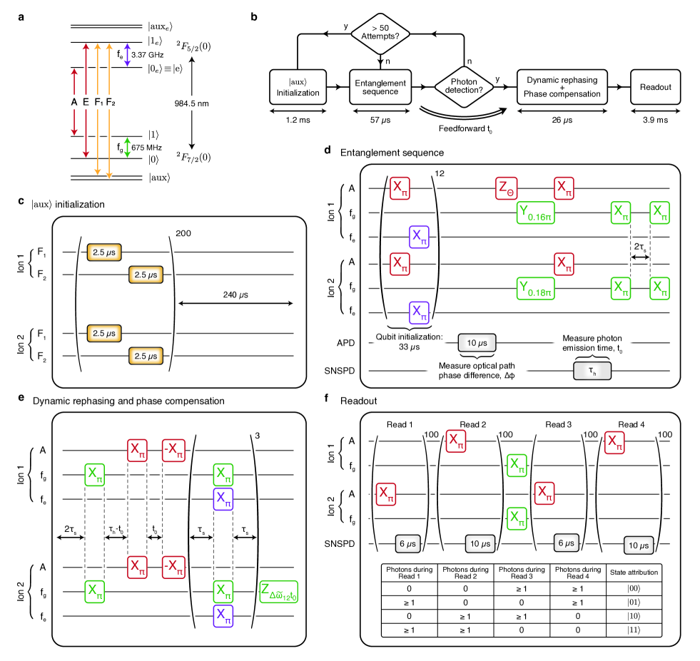
Extended Data Fig. 5: Pulse sequence for remote entanglement generation between two ¹⁷¹ Yb spin qubits. a, Energy level structure of ¹⁷¹ Yb ions at zero magnetic field with relevant optical and spin transitions indicated. The $A$ and $E$ optical transitions have polarization aligned with the cavity mode and are Purcell enhanced. Note that the $\ket{\text{e}}$ state referred to in the main text was labelled $\ket{0_{e}}$ in previous work. b, Flow chart showing steps for remote entanglement generation between Ions 1 and 2 (detailed in subsequent subfigures). c, $\ket{\text{aux}}$ initialization involves 400 pulses, each $2.5~{}\mu$s long, applied alternately to the $F_{1}$ and $F_{2}$ transitions of the two ions, thereby emptying the $\ket{\text{aux}}$ states into the qubit manifold via decay on $E$. d, During the entanglement sequence we first initialize both qubits into $\ket{0}$ via pairs of consecutively applied $\pi$ pulses on $A$ and $f_{e}$ followed by decay on $E$. The optical path phase difference, $\Delta\Phi$, is measured and compensated by a $Z$ rotation by angle $\Theta$ on Ion 1’s $A$ transition (defined in Methods). A weak superposition is prepared on each qubit, the ions are optically excited and entanglement is heralded via detection of a single photon at stochastic time $t_{0}$ in a window of duration $\tau_{h}$. e, After several periods of dynamical decoupling with inter-pulse separation $2\tau_{s}=5.8~{}\mu$s, the spin coherence is rephased for a duration of $\tau_{h}-t_{0}$. Optical coherence is rephased via a delay time of $t_{0}$ between two $A$ transition $\pi$ pulses. A $Z$ rotation is applied to Ion 2’s qubit by angle $\Delta\widetilde{\omega}_{12}t_{0}$ where $\Delta\widetilde{\omega}_{12}$ is the $A$ transition driving frequency difference between the two ions. f, Finally, each Ion’s state is read out via repeated optical excitation on the $A$ transition followed by photodetection. We use a total of four readout periods: the first two are used to determine whether the ions are in the $\ket{1}$ state. A qubit $\pi$ pulse is applied and the final two periods measure the $\ket{0}$ state. States are ascribed according to conditions in the table, all other photodetection outcomes are discarded.

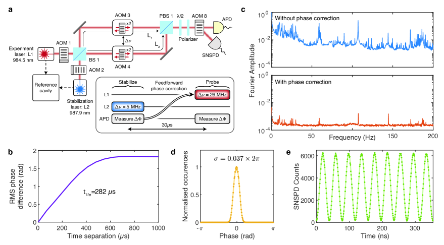
Extended Data Fig. 6: Stabilizing the relative path length between two remote quantum network nodes. a, Simplified optical setup and pulse sequence. The stabilization laser, L2, at 987.9 nm measures the relative optical path phase. This is achieved using AOM 2, 3 and 4 to generate $10~{}\mu$s long pulses with a $2\pi\times 5~{}$MHz frequency difference that travel along the two separate device paths with distances $L_{1}$ and $L_{2}$. AOM 8 routes the pulses to an avalanche photodetector (APD) which detects the resulting beat note phase, thereby measuring the optical path phase difference, $\Delta\Phi$. Subsequently, after a delay of $30~{}\mu$s, the optical phase is probed using L1 at 984.5 nm using pulses generated by AOM 1, 3 and 4 with a $2\pi\times 26$ MHz frequency difference. However, this time, the driving phase of AOM 3 is adjusted in order to correct the optical phase difference by an angle $\Theta$ (defined in Methods), thereby counteracting phase drift and rendering the optical phase constant between consecutive probe periods. The optical phase during each probe period is measured using the APD. b, With the phase correction turned off ($\Theta=0$), we measure the optical phase stability by plotting the RMS difference between values of $\Delta\Phi$ in probe periods of varying time separation, yielding a 1/e phase correlation timescale of $\approx 282~{}\mu$s. c, The resulting Fourier transform of the optical phase noise with the correction, $\Theta$, turned off and on are shown in the top and bottom panels, respectively. d, With the phase stabilization turned on, a normalized histogram of the optical phases during the probe periods yields a Gaussian distribution with standard deviation $0.037\times 2\pi$ rad, corresponding to a limitation in the entangled state fidelity of $\mathcal{F}<0.987$. e, The probe pulses are attenuated to the single-photon level and detected using a superconducting nanowire single photon detector (SNSPD), the resulting contrast of 0.944 verifies that SNSPD timing jitter does not contribute significantly to these measurements.

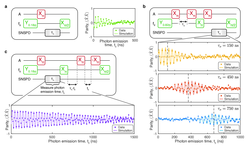
Extended Data Fig. 7: Influence of photonic coherence in entanglement heralding protocols. a, Ramsey entanglement scheme, reproduced from Fig. 2b, Panel ①. The entangled state coherence is probed via a measurement of the $X$-basis parity expectation value, $\langle\hat{X}\hat{X}\rangle$, correlated with the photon emission time, $t_{0}$. The coherence oscillates at the ions’ optical frequency difference, $\Delta\omega_{12}\approx 2\pi\times 31~{}$MHz and undergoes a Gaussian envelope decay with $185\pm 15$ ns timescale, limited by the ions’ optical Ramsey coherence times. b, In this sequence, prior to entanglement heralding, optical phase is accumulated for a fixed duration, $\tau_{0}$, between two consecutive $A$ transition $\pi$ pulses. After a qubit $\pi$ pulse, the ions are excited and, during subsequent free evolution, the optical phase is compensated. Maximal coherence occurs when a heralding photon is detected at $t_{0}=\tau_{0}$. The three panels plot measurement results with $\tau_{0}=$150, 450 and 750 ns from top to bottom, respectively. We see that the coherence still exhibits Gaussian decay limited by the optical Ramsey coherence time. c, Using the dynamic rephasing protocol described in the main text, we observe a significant increase in heralded coherence which exhibits exponential decay with a $1/e$ timescale of $970\pm 30~{}$ns, now limited by the Purcell-enhanced optical lifetimes of the two ions. In all cases, markers and solid lines correspond to experimental data and simulation, respectively, as detailed in Supplementary Information Section .7.

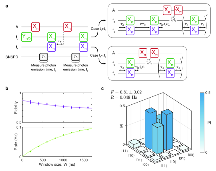
Extended Data Fig. 8: Entanglement heralding between two remote ¹⁷¹Yb ions using a two photon protocol. a, Pulse sequence for remote entanglement generation. Each qubit is prepared in a superposition state, $1/\sqrt{2}(\ket{0}+\ket{1})$, and optically excited in two rounds, separated by a qubit $\pi$ pulse. Photon detections in both rounds at stochastic times $t_{0}$ and $t_{1}$ (measured relative to the start of their respective heralding windows) carve out $\ket{00}$ and $\ket{11}$, respectively, thereby heralding entanglement. Subsequently, a dynamical decoupling sequence is applied with inter-pulse spacing $2\tau_{s}=5.8~{}\mu$s. In cases where $t_{1}<t_{0}$ optical and spin coherences are rephased for durations $\tau_{h}-t_{0}+t_{1}$ and $t_{0}-t_{1}$, respectively, after an even number of dynamical decoupling periods. In cases where $t_{1}>t_{0}$ optical and spin coherences are rephased for durations $\tau_{h}-t_{1}+t_{0}$ and $t_{1}-t_{0}$, respectively, after an odd number of dynamical decoupling periods. Note that we also apply a $Z$ rotation to Ion 2’s qubit by an angle $\Delta\widetilde{\omega}_{12}(t_{0}-t_{1})$ (not labelled). b, Entanglement rate and fidelity plotted against window size, W, where heralding events are accepted under the condition $|t_{1}-t_{0}|<W/2$. The smallest window size, $W=200~{}$ns, leads to a fidelity and rate of $\mathcal{F}=0.84\pm 0.03$ and $\mathcal{R}=17$ mHz, respectively. The largest window size of $W=1.6~{}\mu$s corresponds to a fidelity and rate $\mathcal{F}=0.75\pm 0.02$ and $\mathcal{R}=91$ mHz, respectively. c, Density matrix obtained via maximum likelihood tomography with a window size $W=600~{}$ns (vertical dashed line in b) leading to a fidelity and rate of $\mathcal{F}=0.81\pm 0.02$ and $\mathcal{R}=49$ mHz, respectively.

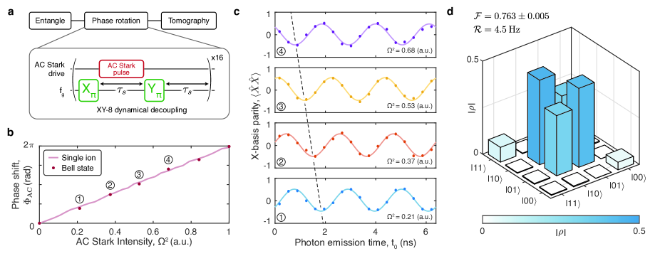
Extended Data Fig. 9: Heralded entanglement between two ¹⁷¹Yb ions in the same nanophotonic cavity. a, The entanglement protocol requires single-qubit $Z$ rotations which cannot be achieved using global microwave driving. Instead, we utilize a differential AC Stark shift of the qubits consisting of an optical pulse with Rabi frequency $\Omega$ which is oppositely detuned from the two ions’ optical transition frequencies. We embed the AC Stark pulses in every alternate period of an XY-8 dynamical decoupling sequence, thereby preserving qubit coherence whilst simultaneously accumulating a differential phase. The sequence consists of $32~{}\pi$ pulses separated by $2\tau_{s}=5.8~{}\mu$s; we vary the differential phase by adjusting the AC Stark intensity which scales with $\Omega^{2}$. b, We verify the performance of the AC Stark control in two ways. First, we independently initialize each qubit in a superposition state, apply the AC Stark sequence, and measure the spin quadratures $\langle\hat{X}\rangle$ and $\langle\hat{Y}\rangle$. We calculate the difference between the two qubits’ phase rotations, $\Phi_{\text{AC}}$, and plot this for different AC Stark intensity values, $\Omega^{2}$ (solid line). We also probe the differential phase using heralded Bell states, detailed in c (markers), these independently derived measurements exhibit a close correspondence. c, After heralding an entangled state, we apply an AC Stark sequence prior to measurement. This adds a quantum phase to our heralded Bell state and a corresponding phase shift in the parity oscillation of coherence with photon emission time, $t_{0}$. We measure this phase shift for different AC Stark intensity values, $\Omega^{2}$; the four parity oscillations correspond to the labelled markers in b. d, Finally, we dynamically adjust the AC Stark intensity in each experiment to counteract the stochastic heralding phase $\Delta\widetilde{\omega}_{13}t_{0}$, thereby rendering the entangled state coherence independent of photon emission time. We accept photons in a $500~{}$ns window and perform maximum likelihood tomography on the quantum state. We plot the resulting density matrix which has a fidelity of $\mathcal{F}=0.763\pm 0.005$, the heralding rate is $\mathcal{R}=4.5$ Hz.

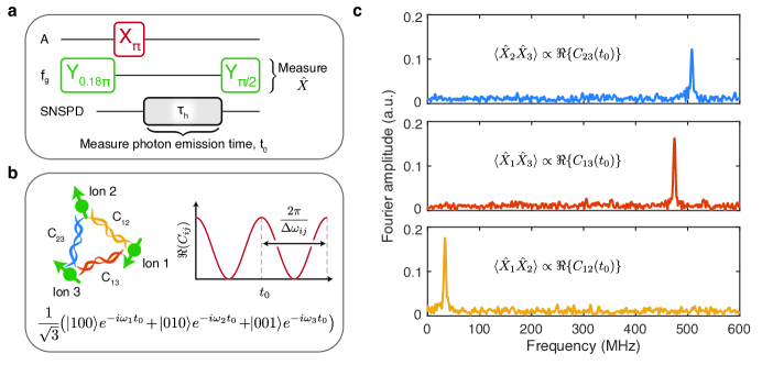
Extended Data Fig. 10: Coherence in tripartite W states between three remote ¹⁷¹Yb ions. a, Tripartite W states are generated using a single photon heralding protocol, whereby each Ion’s qubit is prepared in a weak superposition state, all three ions are resonantly optically excited and entanglement is heralded by the detection of a single photon at stochastic time $t_{0}$. Subsequently, all three qubits are read out in the $X$ basis. b, The tripartite W state heralded using this protocol is an equally weighted superposition of single qubit excitations, each with a quantum phase depending on the optical transition frequency of the excited qubit, $\omega_{i}$, multiplied by $t_{0}$. There are six quantum coherences, $C_{ij}=\Tr\{\hat{\rho}\ket{01}_{ij}\bra{10}_{ij}\otimes\ket{0}_{k}\bra{0}_{k}\}$, where $i,j,k$ correspond to permutations of qubits 1, 2 and 3. We note that the real part of the coherence term $\Re\{C_{ij}\}$ will exhibit oscillations at the optical frequency difference between Ions $i$ and $j$ with photon measurement time, i.e. $\Re\{C_{ij}(t_{0})\}\propto\cos(\Delta\omega_{ij}t_{0})$ where $\Delta\omega_{ij=}\omega_{j}-\omega_{i}$. c, We probe the time dependence of these coherence terms by measuring two-qubit $X$-basis parity expectation values and noting that, for the ideal W state, $\langle\hat{X}_{i}\hat{X}_{j}\rangle\propto\Re\{C_{ij}(t_{0})\}$. We plot the Fourier transform of each partial trace, the three panels correspond to $C_{23},~{}C_{13}$ and $C_{12}$ from top to bottom. In each case we observe an oscillation at the corresponding optical frequency difference, i.e. $\approx 2\pi\times 508$ MHz, $\approx 2\pi\times 475$ MHz and $\approx 2\pi\times 34$ MHz, respectively. Note that the ions’ optical frequencies drift slowly over week-long timescales, hence $\Delta\omega_{12}$ is slightly different here compared to Fig. 2.

Methods

Setup

Extended Data Fig. 4 provides a detailed schematic of the experimental setup.

Each device consists of a YVO₄ chip with nanophotonic cavities fabricated via focused ion beam milling, and microwave coplanar waveguides fabricated by electron-beam lithography Zhong:16 . The devices are mounted in separate setups on the still plate of a ³He cryostat (Bluefors LD-He250) with base temperature of $\approx 0.5$ K. These setups enable optical coupling to fibre, microwave coupling to coax lines, nitrogen-condensation tuning of the optical resonances, and magnetic field cancellation via superconducting coils Kindem2020a .

Optical control is achieved with the setup in Extended Data Fig. 4a. The Ions’ $A$ transitions are addressed by a continuous-wave titanium sapphire laser (L1, M2 Solstis), divided into two paths at a beamsplitter (BS 1). Each path is modulated by a shutter setup (AOM 3 and AOM 4, respectively) containing two free-space acousto-optic modulators (AOMs) in double-pass configuration, thus enabling pulse generation with $\sim 10~{}$ns rise time, single-photon-level extinction, and fast frequency tuning with $400~{}$MHz bandwidth. An additional setup (AOM 5) is used to simultaneously address Ions 1 and 3 in Device 1 (described later). A laser at 987.9 nm (L2, Moglabs Cateye) is used for phase stabilization; it is distributed into the two optical paths via the second input port of BS 1. AOM 1 and AOM 2 select between L1 and L2, depending on the required wavelength. Additional optical transitions ($F_{1}$ and $F_{2}$, Extended Data Fig. 5a) are driven via lasers L3 and L4 (Toptica DL Pro) modulated by AOM 6 and AOM 7 for Device 1 and Device 2, respectively. Setup AOM 6 has a larger bandwidth (600 MHz), enabling both Ion 1 and Ion 3’s transitions to be alternately addressed during the initialization sequence (Extended Data Fig. 4c). Lasers L1 and L2 are stabilized to a reference cavity (Stable Laser Systems) via Pound-Drever-Hall locking Drever1983 . L3 and L4 are stabilized via frequency-offset locking to L1.

The photodetection (output) paths associated with each device are separated from the input via 99:1 beamsplitters, they pass through electronic polarization controllers (OZ Optics EPC) and are combined into the same spatial mode by a polarizing beamsplitter (PBS 1), albeit in orthogonal polarization states. AOM 8 routes light to a detection setup for entanglement heralding and readout or an avalanche photodetector (APD, Laser Components A-CUBE-S500-240) to measure the path phase difference.

There are three different detection setup configurations used in this work (Extended Data Fig. 4b). Setup 1 consists of a single superconducting nanowire single photon detector (SNSPD, Photonspot) and is used to herald entangled states between two ions within the same device (Supplementary Information Section .12). Setup 2 is used for bipartite remote entanglement distribution; it uses a time-delayed interferometer combined with a single SNSPD and can herald entangled states with the same efficiency as more conventional two detector setups Moehring2007 . Specifically, the orthogonally polarized photonic modes from the two devices are mixed via a 45 degree rotation and second polarizing beamsplitter (PBS 2), leading to a spin-photon entangled state:

$$\begin{split}\ket{\psi(t)}&=1/2(\ket{10}+\ket{01}e^{-i\Delta\omega_{12}t})\ket{H}\\ &+1/2(\ket{10}-\ket{01}e^{-i\Delta\omega_{12}t})\ket{V},\end{split}$$ (4)

where $\ket{V}$ is the photonic mode associated with the upper (fibre coupled) arm of the interferometer, and $\ket{H}$ corresponds to the lower (free space) arm. At this stage, a common approach is to place two SNSPDs at the output ports of PBS 2: depending on which detector clicks, opposite parity Bell states would be heralded. However, due to the optical frequency difference between Ions 1 and 2, a propagation delay of duration $\Delta t=\pi/\Delta\omega_{12}$ prior to photodetection can be used to invert the entangled state parity. We introduce a calibrated fibre delay-line into the upper arm of the interferometer before combining the two paths on a third polarizing beamsplitter (PBS 3). At this stage the spin-photon entangled state is given by:

$$\begin{split}\ket{\psi(t)}&=1/2(\ket{10}+\ket{01}e^{-i\Delta\omega_{12}t})(\ket{H}+\ket{V})\end{split}$$ (5)

where $\ket{H}$ and $\ket{V}$ correspond to orthogonally polarized photonic modes in the same spatial output port of PBS 3. We can now deterministically herald Bell states:

$$\ket{\psi(t)}=1/2(\ket{10}+\ket{01}e^{-i\Delta\omega_{12}t})$$ (6)

using a single detector. Setup 3 is used for tripartite entangled state generation and consists of two SNSPDs after PBS 2. Depending on which detector clicks, we apply a conditional $Z$ rotation to Ion 2’s qubit, thereby eliminating the detector-dependent parity phase shift.

The microwave control setup is depicted in Extended Data Fig. 4e. Microwave pulses at $\approx 2\pi\times 3.37$ GHz, used to drive the excited state spin transition, are generated with RF signal generators (SRS SG380), microwave switches, and amplifiers (Minicircuits ZHL-16W-43-S+). Control pulses at the $\approx 2\pi\times 675$ MHz ground state qubit transition frequencies are generated via heterodyne mixing of a target waveform at $\approx 2\pi\times 275$ MHz with a local oscillator at $2\pi\times 950$ MHz (Holzworth HS 9002A), bandpass-filtering to remove the image frequencies and amplification (Amplifier Research 10U1000 for Device 1 and Minicircuits ZHL-20W-13SW+ for Device 2).

The experiment is operated by a Quantum Machines OPX control platform which generates all pulses for optical and spin driving. Both SNSPDs and the APD are connected to the two OPX input ports (one SNSPD and the APD share a single port via a diplexer). This enables measurement-based feed-forward using single photon detection times, necessary for the dynamic rephasing and phase compensation protocols described in the main text.

Phase Stabilization

The phase difference between the combined laser excitation and photodetection paths associated with the two devices is imprinted on heralded Bell states and therefore requires active stabilization cabrillo1999 ; Minar2008 . A simplified version of the experimental setup relevant to this section (with the devices excluded) is presented in Extended Data Fig. 6a whereby the two optical paths, with lengths $L_{1}$ and $L_{2}$, form an interferometer. The relevant Bell state phase is $\Delta\Phi_{\lambda_{1}}=2\pi(L_{1}-L_{2})/\lambda_{1}$ where $\lambda_{1}=984.5~{}$nm is the experiment wavelength.

We measure the relative path phase using detuned optical pulses at $\lambda_{2}=987.9~{}$nm , yielding $\Delta\Phi_{\lambda_{2}}=2\pi(L_{1}-L_{2})/\lambda_{2}$. This off-resonant light reflects from the devices without exciting the cavity mode, thereby minimizing heating. Specifically, AOM 2, AOM 3 and AOM 4 are used to generate $10~{}\mu s$ light pulses from laser L2, with a $5~{}$MHz frequency difference travelling in two separate arms of the interferometer. When recombined on PBS 1 and measured on the APD, the phase of the resulting heterodyne beat note yields $\Delta\Phi_{\lambda_{2}}$.

We can use $\Delta\Phi_{\lambda_{2}}$ as an approximate measure for $\Delta\Phi_{\lambda_{1}}$, under the condition that their difference is static, i.e. $\Delta\Phi_{\lambda_{1}}-\Delta\Phi_{\lambda_{2}}=2\pi(L_{1}-L_{2})\left(\frac{1}{\lambda_{1}}-\frac{1}{\lambda_{2}}\right)=\text{constant}$. Therefore, with $L_{2}-L_{1}\approx 3~{}$m, fluctuation of the optical frequency difference between these two lasers must by much less than $\approx 70~{}$MHz, which is achieved by stabilizing both lasers to a reference cavity via Pound-Drever-Hall (PDH) locking Drever1983 . Hereafter, we will ignore the static difference between these values and drop the subscripts, i.e. $\Delta\Phi\equiv\Delta\Phi_{\lambda_{1},\lambda_{2}}$.

The time dependence of $\Delta\Phi$ is investigated in Extended Data Fig. 6b where we plot the RMS difference between phase measurements of varying separation, yielding a 1/e correlation timescale of $\approx 282~{}\mu$s. Hence, we need to first measure and then correct $\Delta\Phi$ for each entanglement attempt, which is achieved by adjusting the microwave driving phase of AOM 3 during optical control pulses at $\lambda_{1}$.

To demonstrate and verify our ability to stabilize the optical phase difference we use the pulse sequence depicted in Extended Data Fig. 6a (inset). Specifically, during experiment repetition $i$, we first measure the optical phase difference, $\Delta\Phi_{i}$, with a pulse at $\lambda_{2}$, as described previously. Then, we wait for a duration of $30~{}\mu$s before probing the phase using an optical pulse at $\lambda_{1}=984.5~{}$nm, however this time we apply an optical phase correction via AOM 3 of $\Theta=-\Delta\Phi_{i}-\beta(\Delta\Phi_{i}-\Delta\Phi_{(i-1)})$. Note that $\Theta$ includes both a static component ($\Delta\Phi_{i}$) and a linear extrapolation of the phase trajectory ($\beta(\Delta\Phi_{i}-\Delta\Phi_{(i-1)})$), where $\beta$ accounts for the difference in delay time between different pulses.

We use the APD to measure the heterodyne phase during each probe pulse at wavelength $\lambda_{1}$, the Fourier transform of the resulting time-dependent optical phase provides the phase noise frequency spectrum. We plot this spectrum with and without the phase correction ($\Theta$) applied (Extended Data Fig. 6c), and note the reduction in integrated phase noise between these cases. In Extended Data Fig. 6d, we quantify the effectiveness of our phase stabilization by histogramming the optical phases gathered over 20 minutes of integration time with a resulting standard deviation of $\sigma=0.037\times 2\pi~{}$rad. This residual phase variation reduces the coherence of our entangled states, thereby limiting the fidelity to $\mathcal{F}<0.987$. Finally, we attenuate the probe pulses to the single-photon level and measure the resulting beat note using an SNSPD (note that we use an optical frequency difference of $2\pi\times 26~{}$MHz between the two interferometer arms during the $\lambda_{1}$ probe pulse to mimic the ion frequency difference). We histogram the single photon arrival times in Extended Data Fig. 6e with an integration time of 1 minute, the resulting contrast is 0.944. This verifies that SNSPD jitter is not a significant limitation in these experiments.

Detailed Entanglement Sequence

In this section we provide more detail regarding the bipartite remote entanglement sequence. Extended Data Fig. 5a provides a detailed energy level structure with all optical and spin transitions used in this work labelled (see Supplementary Information Section .1 for more detail). The experiment flow is depicted in Extended Data Fig. 5b. We start by depleting the $\ket{\text{aux}}$ states of both ions into the qubit manifold via interleaved optical pulses on $F_{1}$ and $F_{2}$ followed by cavity-enhanced decay on $E$ (Extended Data Fig. 5c). We estimate an initialization fidelity lower-bounded by 0.98 (see Supplementary Information Section .10). Within each heralding attempt, the probability of transferring population into the $\ket{\text{aux}}$ states is relatively small ($\approx 1.2\times 10^{-3}$), we therefore only repeat this step if 50 consecutive heralding attempts have failed.

Next, we initialize the qubits into $\ket{0}$ via consecutive $\pi$ pulses on $A$ and $f_{e}$ followed by cavity-enhanced decay on $E$. This is repeated twelve times yielding qubit initialization fidelities of $0.9976\pm 0.0003$ and $0.9954\pm 0.0008$ for Ions 1 and 2, respectively (Extended Data Fig. 5d).

The phase difference between the two optical paths is measured and stabilized, as described in the previous section.

Next, we herald an entangled state using a single photon protocol. We start by preparing an initial state, $\ket{\psi_{\text{init}}}$, where each qubit is in a weak superposition with probability $\alpha_{i}$ in the $\ket{1}$ state:

$$\ket{\psi_{\text{init}}}=(\sqrt{1-\alpha_{1}}\ket{0}+\sqrt{\alpha_{1}}\ket{1})\otimes(\sqrt{1-\alpha_{2}}\ket{0}+\sqrt{\alpha_{2}}\ket{1}).$$

Both ions are optically excited and an entangled state is heralded by the detection of a single photon which is measured at stochastic times $t_{0}$. The resulting conditional density matrix associated with a photon detection in a window of size $\delta t$ centred at $t_{0}$ is given by Hermans2023 :

$$\hat{\rho}(t_{0})=\\ R_{\text{DC}}\delta t\!\!\!\!\!\!\sum_{i,j\in\{0,1\}}\!\!\!\!\!\!\left(|\bra{ij}\ket{\psi_{\text{init}}}|^{2}\ket{ij}\bra{ij}\right)+\delta t\ket{\psi(t_{0})}\bra{\psi(t_{0})}\\ +\ket{11}\bra{11}\left(\frac{p_{\text{det}}^{(1)}}{T_{1,o}^{(1)}}e^{-t_{0}/T_{1,o}^{(1)}}+\frac{p_{\text{det}}^{(2)}}{T_{1,o}^{(2)}}e^{-t_{0}/T_{1,o}^{(2)}}\right)\alpha_{1}\alpha_{2}\delta t,$$

where we have only considered terms up to and including $\mathcal{O}(\delta t)$ and where $R_{\text{DC}}$ is the noise count rate, $T_{1,o}^{(i)}$ is the optical lifetime of Ion $i$ and $p_{\text{det}}^{(i)}$ is the probability of detecting a photon emitted by Ion $i$, which is assumed to be much less than 1. $\ket{\psi(t_{0})}$ is an unnormalized quantum state given by:

$$\ket{\psi(t_{0})}=a(t_{0})\ket{10}+b(t_{0})\ket{01}e^{-i\phi(t_{0})},$$ (7)

with

$$a(t_{0}) =\sqrt{\frac{p_{\text{det}}^{(1)}\alpha_{1}(1-\alpha_{2})}{T_{1,o}^{(1)}}}e^{-t_{0}/2T_{1,o}^{(1)}},$$ (8)

$$b(t_{0}) =\sqrt{\frac{p_{\text{det}}^{(2)}\alpha_{2}(1-\alpha_{1})}{T_{1,o}^{(2)}}}e^{-t_{0}/2T_{1,o}^{(2)}},$$ (9)

$$\phi(t_{0}) =\Delta\omega_{12}\times t_{0},$$ (10)

where $\Delta\omega_{12}$ is the fluctuating optical frequency difference between Ions 1 and 2. Since $\Delta\omega_{12}$ can be regarded as quasi-static on the timescale of a single heralding attempt, we don’t explicitly label the time dependence and regard it as a shot-to-shot random variable, following a Gaussian distribution. Note that the conditional density matrix, $\hat{\rho}(t_{0})$ is un-normalized, with trace equal to the probability of a photon detection occurring in the window of size $\delta t$. The unconditional density matrix within a photon acceptance window of size $\tau_{A}$ is given by $\hat{\rho}=\langle\int_{0}^{\tau_{A}}dt_{0}\left(\hat{\rho}(t_{0})/\delta t\right)\rangle_{\Delta\omega_{12}}$, and is ensemble-averaged over optical frequency differences. We note that the analytic form of this density matrix incorporates only a limited set of error sources for illustrative purposes. The simulations presented in the main text are derived using a comprehensive numerical model which is presented in Supplementary Information Section .7.

Optimal values of $\alpha_{1}$ and $\alpha_{2}$ are identified in two stages. First, we choose a ratio $\xi=\alpha_{1}/\alpha_{2}=0.79$ which balances the populations associated with $\ket{10}\bra{10}$ and $\ket{01}\bra{01}$ across our acceptance window, i.e. that satisfies $\int_{0}^{\tau_{A}}|a(t_{0})|^{2}dt_{0}=\int_{0}^{\tau_{A}}|b(t_{0})|^{2}dt_{0}$. Then, we sweep $\alpha_{2}$ from 0 to 1 (with $\alpha_{1}$ also varying according to $\alpha_{1}=\xi\alpha_{2}$) and identify a maximum entangled state fidelity. For small values of $\alpha_{2}$, ion emission is suppressed and the entangled state fidelity reduces due to heralding based on noise counts, i.e. $\hat{\rho}(t_{0})\rightarrow R_{\text{DC}}\delta t\sum_{i,j\in\{0,1\}}|\bra{ij}\ket{\psi_{\text{init}}}|^{2}\ket{ij}\bra{ij}$, representing an incoherent mixture of the four classical two-qubit states collapsed from the initial state. For large values of $\alpha_{2}$, occupation of $\ket{11}\bra{11}$ increases which also leads to a reduction in fidelity. Hence, there is an optimal intermediate value of $\alpha_{2}=0.078$ which balances these two competing sources of infidelity.

After heralding an entangled state, we rephase the coherence by counteracting $\phi(t_{0})$ (equation (10)), using a pulse sequence with parameters that are dynamically varied based on the photon arrival time, $t_{0}$ (feedforward). The pulse sequence is described in the main text, however, there are two additional aspects worth noting here. First, we apply two qubit dynamical decoupling periods after the entanglement sequence, prior to rephasing; this provides sufficient time for the experiment control system to determine if any photon detection events occurred and whether to proceed. Secondly, after dynamic rephasing, we mitigate qubit population-basis errors caused by imperfections in the preceding optical $\pi$ pulses. Specifically, we wait for optical decay to deplete the $\ket{e}$ state whilst applying three qubit dynamical decoupling periods to preserve entangled state coherence. The qubit $\pi$ pulses are synchronised with excited state microwave $\pi$ pulses applied to the $f_{e}$ transition, thereby ensuring that population in the excited state manifold always decays to the correct ground state. Note that this procedure will not improve the coherence of heralded Bell states, only the contrast of diagonal density matrix elements (populations).

Finally, we read out the two qubit state: we apply 100 consecutive optical $\pi$ pulses to Ion 2, each followed by a $6~{}\mu$s photon detection window. The process is repeated for Ion 1 with a $10~{}\mu$s window. Photon detections during these two read periods correspond to population in $\ket{1}$. Then, $\pi$ pulses are applied consecutively to both qubits and the process is repeated, this time any photon detections correspond to population that was originally in $\ket{0}$. The total number of photons in each read period are counted, and the two-qubit state is ascribed according to the table in Extended Data Fig. 5f. In cases where one of these four conditions isn’t satisfied (e.g. no photons detected), the experiment result is discarded. This leads to a readout efficiency of approximately 0.18 and an average readout fidelity of 0.93.

The duration of each step in the experiment sequence is listed in Extended Data Fig. 5b, the total time per entanglement attempt is $81~{}\mu$s, this includes the effect of $\ket{\text{aux}}$ initialization which, on average, contributes $24~{}\mu$s per attempt.

Maximum Likelihood Tomography

We use maximum likelihood quantum state tomography to characterize entangled states. This involves finding a predicted density matrix that best describes the experimentally observed results James2001 ; Hradil1997 .

We start by reading out our entangled state in 9 cardinal two-qubit Pauli bases along $X$, $Y$ and $Z$. Each measurement basis (denoted $(ij)$, with $i,j\in\{X,Y,Z\}$) yields four photon count numbers $N^{(ij)}_{00},~{}N^{(ij)}_{01},~{}N^{(ij)}_{10},~{}N^{(ij)}_{11}$, corresponding to readout of the four 2-qubit measurement basis eigenstates, $\ket{00},~{}\ket{01},~{}\ket{10},~{}\ket{11}$, respectively. Figure 2c shows the resulting populations for the $XX$, $YY$ and $ZZ$ measurement bases, the other 6 bases ($XY,~{}XZ,~{}YX,~{}YZ,~{}ZX,~{}ZY$) are not shown but are included in the maximum likelihood reconstruction that follows.

We assume that the results of each measurement basis are multinomially distributed such that the likelihood of a model density matrix, $\hat{\rho}$, is given by Bernien2013 :

$$\begin{split}\mathcal{L}^{(ij)}(\hat{\rho})=&\frac{N^{(ij)}!}{N^{(ij)}_{00}!N^{(ij)}_{01}!N^{(ij)}_{10}!N^{(ij)}_{11}!}\times\\ &\left[n^{(ij)}_{00}\right]^{N^{(ij)}_{00}}\left[n^{(ij)}_{01}\right]^{N^{(ij)}_{01}}\left[n^{(ij)}_{10}\right]^{N^{(ij)}_{10}}\left[n^{(ij)}_{11}\right]^{N^{(ij)}_{11}},\end{split}$$ (11)

where $N^{(ij)}=\sum_{a\in\{00,01,10,11\}}N^{(ij)}_{a}$, and $\{n^{(ij)}_{a}\}$ are the predicted populations of each measurement basis eigenstate according to the model density matrix. For example, if we were to consider the $\ket{00}$ eigenstate in the $XX$ basis, the value of $n^{(XX)}_{00}=\Tr\{\ket{00}\bra{00}\hat{U}^{{\dagger}}_{XX}\hat{\rho}\hat{U}_{XX}\}$ where $\hat{U}_{XX}$ rotates both qubits into the $X$ basis.

In order to account for readout infidelity, we need to define predicted population measurements $\{p^{(ij)}_{a}\}$ which are related to the ideal populations $\{n^{(ij)}_{a}\}$ by a readout transformation matrix $R_{a,b}$ which satisfies: $p^{(ij)}_{a}=\sum_{b\in\{00,01,10,11\}}R_{a,b}n^{(ij)}_{b}$. Here, $R_{a,b}$ is the probability of measuring state $\ket{a}$, given that the two qubits were perfectly prepared in state $\ket{b}$, and $a,b\in\{00,01,10,11\}$ Nguyen2019 . With this readout correction, the predicted $\ket{00}$ measured population in the $XX$ basis becomes:

$$\begin{split}p^{(XX)}_{00}=&\Tr\{\ket{00}\bra{00}\hat{U}^{{\dagger}}_{XX}\hat{\rho}\hat{U}_{XX}\}R_{00,00}+\\ &\Tr\{\ket{01}\bra{01}\hat{U}^{{\dagger}}_{XX}\hat{\rho}\hat{U}_{XX}\}R_{00,01}+\\ &\Tr\{\ket{10}\bra{10}\hat{U}^{{\dagger}}_{XX}\hat{\rho}\hat{U}_{XX}\}R_{00,10}+\\ &\Tr\{\ket{11}\bra{11}\hat{U}^{{\dagger}}_{XX}\hat{\rho}\hat{U}_{XX}\}R_{00,11},\end{split}$$

similar expressions are used for the other populations and other readout bases, but are not listed here for brevity. We use a redefined likelihood function where $\{n_{a}^{(ij)}\}$ in equation (11) are replaced with $\{p_{a}^{(ij)}\}$. We assume that $N^{(ij)}$ is sufficiently large that we can approximate the likelihood function with a normal distribution:

$$\mathcal{L}^{(ij)}(\hat{\rho})\propto\prod_{a\in\{00,01,10,11\}}e^{-\left[\frac{\left(\tilde{n}_{a}^{(ij)}-p_{a}^{(ij)}\right)^{2}N^{(ij)}}{2\tilde{n}_{a}^{(ij)}\left(1-\tilde{n}_{a}^{(ij)}\right)}\right]},$$

where $\tilde{n}_{a}^{(ij)}$ are normalized measured populations, i.e., $\tilde{n}_{a}^{(ij)}=N^{(ij)}_{a}/N^{(ij)}$. The likelihood function for all 9 measurement bases is simply the product of these individual basis likelihood functions:

$$\mathcal{L}(\hat{\rho})=\prod_{i,j\in\{X,Y,Z\}}\mathcal{L}^{(ij)}(\hat{\rho}).$$

Finally, we take the log-likelihood, leading to:

$$\mathcal{L}(\hat{\rho})=\!\!\!\!\!\!\!\!\!\sum_{i,j\in\{X,Y,Z\}}\sum_{a\in\{00,01,10,11\}}\left[\frac{-\left[\tilde{n}_{a}^{(ij)}-p_{a}^{(ij)}\right]^{2}N^{(ij)}}{2\tilde{n}_{a}^{(ij)}\left(1-\tilde{n}_{a}^{(ij)}\right)}\right].$$

We use the convex optimization package CVX gb08 ; cvx in Matlab to find the density matrix, $\hat{\rho}$, which maximizes the log-likelihood. Error estimates are obtained using a bootstrapping protocol. This involves using our predicted density matrix to generate 1000 simulated sets of experimental results, each of which is used to predict a new density matrix via the maximum likelihood analysis. Errors are quoted as standard deviations of observables derived from this set of density matrices.

A similar approach is used for estimating the three-qubit density matrix of tripartite entangled states. In this case, measurements are performed in all 27 cardinal three-qubit Pauli bases along $X$, $Y$ and $Z$, and the readout matrix $R_{a,b}$ now transforms three-qubit populations i.e. $a,b\in\{000,001,010,011,100,101,110,111\}$.

Single qubit tomography, used in the teleportation experiments, is performed via a direct reconstruction from measurements in the $X,~{}Y$ and $Z$ bases. Specifically, the predicted density matrix is given by:

$$\hat{\rho}=\frac{1}{2}\left[\mathbb{I}+\langle\hat{X}\rangle\hat{X}+\langle\hat{Y}\rangle\hat{Y}+\langle\hat{Z}\rangle\hat{Z}\right],$$

where $\hat{X}$, $\hat{Y}$, and $\hat{Z}$ are the Pauli matrices, and $\langle\hat{X}\rangle$, $\langle\hat{Y}\rangle$, and $\langle\hat{Z}\rangle$ are measured populations which have been corrected for readout infidelity.

Raw data for all tomography measurements in this work are presented in Supplementary Information Section .13, along with the corresponding readout transformation matrices ($R_{a,b}$) and resulting complex-valued predicted density matrices, $\hat{\rho}$.

Teleportation Protocol Details

To demonstrate the probabilistic teleportation protocol, Ion 2 is prepared in the target state, $\ket{\psi_{T}}=\cos(\theta_{T}/2)\ket{0}+e^{i\phi_{T}}\sin(\theta_{T}/2)\ket{1}$, by application of consecutive $Y$ and $Z$ rotations through angles $\theta_{T}\in[0,\pi]$ and $\phi_{T}\in[0,2\pi]$, respectively, to the initial state, $\ket{0}$. These angles encode all possible single qubit pure states. While this method of state preparation relies on classical knowledge of the target state by the sender, we emphasize that this is not a requirement of the protocol. Namely, Ion 2 could be provided with an unknown quantum state (for instance, by means of a SWAP gate applied to an auxiliary qubit) and the protocol would operate in the same manner.

Ion 1 is prepared in the initial state $1/\sqrt{2}(\ket{0}+\ket{1})$. Subsequently, both ions are optically excited in two successive rounds, separated by a qubit $\pi$ pulse. Single photon detections in each round, at times $t_{0}$ and $t_{1}$ (measured relative to the start of each heralding window), lead to an entangled two qubit state:

$$\ket{\psi(t_{0},t_{1})}=\cos(\theta_{T}/2)\ket{10}\\ +e^{i(\phi_{T}+\phi(t_{0},t_{1}))}\sin(\theta_{T}/2)\ket{01},$$

where $\phi(t_{0},t_{1})=\Delta\omega_{12}(t_{0}-t_{1})$. We note that optical path phase, $\Delta\Phi$, accumulated by the first photon is cancelled by the second; hence, active phase stabilization is not required for these measurements. The stochastic phase, $\phi(t_{0},t_{1})$, is corrected using the pulse sequences presented in the right panels of Extended Data Fig. 8a which contain dynamically adapted parameters that depend on both photon detection times. Specifically, after the heralding windows we apply a dynamical decoupling sequence to the qubits consisting of five $\pi$ pulses. In cases where $t_{1}<t_{0}$, we correct the stochastic phase after the second qubit $\pi$ pulse by waiting for a duration $\tau_{h}-t_{0}+t_{1}$ before applying two optical $\pi$ pulses separated by a delay time of $t_{0}-t_{1}$ to both ions. These two delays correct qubit and optical dephasing, respectively, that occurred during the preceding heralding windows. In cases where $t_{1}>t_{0}$ the correction happens after the third qubit $\pi$ pulse, the spin and optical coherences are rephased for durations of $\tau_{h}-t_{1}+t_{0}$ and $t_{1}-t_{0}$, respectively. At this stage, the two-qubit quantum state is given by:

$$\ket{\psi(t_{0},t_{1})}=\cos(\theta_{T}/2)\ket{01}\\ +\sin(\theta_{T}/2)e^{i(\phi_{T}+\Delta\widetilde{\omega}_{12}(t_{0}-t_{1}))}\ket{10}.$$

Finally, we apply a $Z$ rotation to Ion 1’s qubit by an angle $-\Delta\widetilde{\omega}_{12}(t_{0}-t_{1})$, thereby yielding the state:

$$\ket{\psi}=\cos(\theta_{T}/2)\ket{01}+\sin(\theta_{T}/2)e^{i\phi_{T}}\ket{10}.$$

The remaining steps in the protocol are detailed in the main text.

Single Device Multiplexing

During entanglement experiments involving Ions 1 and 3 (which are within the same device), both Ions’ optical transitions are driven simultaneously. This is achieved using setup AOM 5 which consists of a single AOM in double-pass configuration, driven at half the ion frequency difference ($\approx 2\pi\times 237.5~{}$MHz) and aligned to accept both $0^{\text{th}}$ and $-1^{\text{st}}$ orders (Extended Data Fig. 4d). This generates two optical tones separated by $\approx 2\pi\times 475~{}$MHz for driving Ions 1 and 3 in a manner that’s passively phase-stable. We also note that photons emitted by these ions travel through the same optical fibre before reaching the detection setup, hence no active phase stabilization of the optical path difference is required.

Global microwave driving precludes single-qubit $Z$ gates which are necessary for correcting stochastic phases, $\Delta\widetilde{\omega}_{13}t_{0}$, introduced during the heralding protocol (here $\Delta\widetilde{\omega}_{13}$ is the optical drive frequency difference between Ions 1 and 3, $t_{0}$ is the photon emission time). Instead, we leverage the optical inhomogeneity to implement a differential AC-stark shift on the two qubits using the protocol detailed in chen2020 . Specifically, we apply an XY-8 dynamical decoupling sequence consisting of 32 qubit $\pi$ pulses with inter-pulse separation $2\tau_{s}=5.8~{}\mu$s (total duration $186~{}\mu$s). During every alternate free evolution period we apply an optical pulse with Rabi frequency $\Omega$ which is detuned by $\Delta\omega_{\text{AC}}^{(1)}\approx-2\pi\times 50$ MHz from Ion 1 and $\Delta\omega_{\text{AC}}^{(3)}\approx+2\pi\times 425$ MHz from Ion 3 (Extended Data Fig. 9a). At the end of the decoupling sequence, this leads to a relative phase shift between the two qubits of $\Phi_{\text{AC}}\approx 8\Omega^{2}\tau_{s}(1/\Delta\omega_{\text{AC}}^{(3)}-1/\Delta\omega_{\text{AC}}^{(1)})$. We probe $\Phi_{\text{AC}}$ by performing single-qubit measurements of the $X$ and $Y$ spin quadratures of each ion (Extended Data Fig. 9b, solid line). In each heralding experiment, the AC shark shift, which scales with $\Omega^{2}$, is dynamically adjusted such that the resulting $\Phi_{\text{AC}}$ counteracts the stochastic phase $\Delta\widetilde{\omega}_{13}t_{0}$ (Supplementary Information Section .12).

Global microwave driving also complicates tomography, where independent rotations of each qubit are required (for instance when measuring in the $ZX$ basis). These rotations are generated via global $X$ and $Y$ control combined with local $Z$-rotations. For instance, applying the following sequence of pulses:

$$Y_{\pi/4}~{}Z^{(1)}_{+\pi/2}~{}Z^{(3)}_{-\pi/2}~{}X_{\pi/4},$$

followed by population basis readout will lead to a measurement in the $Z$ basis for Ion 1 and $X$ basis for Ion 3. Here, $\alpha^{(i)}_{\theta}$ corresponds to $\theta$ pulse applied about the $\alpha$ axis to qubit $i$, if no superscript is given, the pulse is global. Since the qubit frequency difference for Ions 1 and 3 is relatively large ($\approx 2\pi\times 1.13$ MHz) we implement the local $\pm\pi/2$ $Z$ rotations via a 440 ns wait. The fidelity of this approach is limited by the spin Ramsey coherence time, for smaller frequency differences the AC stark shift approach introduced previously can be used.

Tripartite Entanglement Protocol

This section provides additional detail related to the three-ion entanglement protocol. After initializing all three qubits in $\ket{0}$, each ion is prepared in a weak superposition state:

$$\begin{split}\ket{\psi}=&(\sqrt{1-\alpha_{1}}\ket{0}+\sqrt{\alpha_{1}}\ket{1})\otimes\\ &(\sqrt{1-\alpha_{2}}\ket{0}+\sqrt{\alpha_{2}}\ket{1})\otimes(\sqrt{1-\alpha_{3}}\ket{0}+\sqrt{\alpha_{3}}\ket{1}),\end{split}$$

with $\alpha_{1}=0.079$, $\alpha_{2}=0.078$, and $\alpha_{3}=0.079$. All three ions are simultaneously, resonantly optically excited and entanglement is heralded on detection of a single photon. This carves out the optically dark component, $\ket{000}$. Components with more than one qubit spin excitation (for instance $\ket{110}$) are suppressed by choosing $\alpha_{1},~{}\alpha_{2},~{}\alpha_{3}\ll 1$. Note that compared to the bipartite entanglement case, the resulting states will have lower fidelity, i.e., assuming that the same value of $\alpha$ is used for all ions, the two ion Bell state fidelity will be upper-bounded by $1-\alpha$, whereas the three ion W state fidelity will be upper-bounded by $(1-\alpha)^{2}$. Ignoring this source of infidelity and assuming that the values of $\alpha_{i}$ are chosen to counteract differences in lifetime and detection efficiency between the three ions, we can approximate the heralded state as:

$$\ket{\psi(t_{0})}=\\ \frac{1}{\sqrt{3}}\left(\ket{100}e^{-i\omega_{1}t_{0}}+\ket{010}e^{-i\omega_{2}t_{0}}+\ket{001}e^{-i\omega_{3}t_{0}}\right),$$

where $t_{0}$ is the photon detection time and $\omega_{i}$ is the optical frequency of Ion $i$.

We probe these time-dependent coherences in Extended Data Fig. 10, where we read out all three qubits in the $X$ basis. The W state has six quantum coherences, $C_{ij}=\Tr\{\hat{\rho}\ket{01}_{ij}\bra{10}_{ij}\otimes\ket{0}_{k}\bra{0}_{k}\}$, where $i,j,k$ correspond to permutations of qubits 1, 2 and 3. We note that the real part of the coherence term $\Re\{C_{ij}\}$ will exhibit an oscillation at the optical frequency difference between Ions $i$ and $j$ with respect to photon measurement time, and, for the ideal W state, will be proportional to the two-qubit $X$-basis parity expectation value, i.e. $\Re\{C_{ij}(t_{0})\}\propto\cos(\Delta\omega_{ij}t_{0})\propto\langle\hat{X}_{i}\hat{X}_{j}\rangle$. We plot the Fourier transform of each parity measurement in Extended Data Fig. 10c where the three panels correspond to $C_{23},~{}C_{13}$ and $C_{12}$ from top to bottom. We observe parity oscillations at $\approx 2\pi\times 508$ MHz, $\approx 2\pi\times 475$ MHz and $\approx 2\pi\times 34$ MHz, respectively which match the ion frequency differences. Note that the ions’ optical frequencies exhibit slow drift on the timescale of several weeks, hence $\Delta\omega_{12}$ is slightly different here compared to the bipartite entanglement experiments in Fig. 2.

To prepare deterministic entangled states, after the heralding window, we apply the dynamic rephasing protocol consisting of a qubit $\pi$ pulse, a delay time $\tau_{h}-t_{0}$ for spin rephasing (where $\tau_{h}$ is the heralding window size), and a pair of optical $\pi$ pulses separated by $t_{0}$. All of these pulses are applied to the three ions simultaneously. After an additional qubit $\pi$ pulse the quantum state is given by:

$$\ket{\psi(t_{0})}=\frac{1}{\sqrt{3}}(\ket{100}+\ket{010}e^{-i\Delta\widetilde{\omega}_{12}t_{0}}+\ket{001}e^{-i\Delta\widetilde{\omega}_{13}t_{0}}),$$

where $\Delta\widetilde{\omega}_{ij}$ is the frequency difference between lasers used to drive Ions $i$ and $j$. We can see that there are two residual stochastic quantum phases that need to be compensated. First we apply an AC Stark sequence, described in the previous section, to correct the stochastic phase $\Delta\widetilde{\omega}_{13}t_{0}$ between Ions 1 and 3, leading to:

$$\ket{\psi(t_{0})}=\frac{1}{\sqrt{3}}\left(\ket{100}+\ket{010}e^{-i\phi(t_{0})}+\ket{001}\right),$$

where

$$\phi(t_{0})=t_{0}\left(\Delta\widetilde{\omega}_{12}+\Delta\widetilde{\omega}_{13}\frac{\Delta\omega_{\text{AC}}^{(3)}}{\Delta\omega_{\text{AC}}^{(1)}-\Delta\omega_{\text{AC}}^{(3)}}\right),\\$$

and $\Delta\omega_{\text{AC}}^{(i)}$ is the detuning of the optical AC Stark tone from Ion $i$. Then, we apply a phase shift to Ion 2’s qubit drive by an angle $\Phi=\phi(t_{0})$ to cancel the residual stochastic phase, leading to the canonical, tripartite W state:

$$\ket{\text{W}}=\frac{1}{\sqrt{3}}\left(\ket{100}+\ket{010}+\ket{001}\right).$$

Independent basis rotations are applied to the three qubits prior to readout, the process for performing these rotations on qubits within the same device is also described in the previous section.

oneΔ

Supplementary Information

.1 Energy Levels

Extended Data Fig. 5a depicts the energy level structure and transitions relevant to this work at zero magnetic field. We consider 4f–4f transitions between the ${}^{2}F_{7/2}$ ground state multiplet and the ${}^{2}F_{5/2}$ excited state multiplet. Specifically, between the lowest lying crystal field levels (${}^{2}F_{7/2}(0)\leftrightarrow^{2}F_{5/2}(0)$) at 984.5 nm. These levels are each Kramers doublets consisting of an effective electronic spin $1/2$. The hyperfine interaction with the ¹⁷¹Yb nuclear spin with $I=1/2$ lifts the Kramers degeneracy. Of particular relevance are the $F=0,~{}m_{F}=0$ singlet and $F=1,~{}m_{F}=0$ triplet energy levels in the ground state: $\ket{0}=\frac{1}{\sqrt{2}}(\ket{\uparrow\Downarrow}-\ket{\downarrow\Uparrow})$ and $\ket{1}=\frac{1}{\sqrt{2}}(\ket{\uparrow\Downarrow}+\ket{\downarrow\Uparrow})$, respectively, where $\{\ket{\uparrow},\ket{\downarrow}\}$ is the electronic spin and $\{\ket{\Uparrow},\ket{\Downarrow}\}$ is the nuclear spin. These levels are split by $\approx 2\pi\times 675~{}$MHz and form our qubit, which can be driven by an oscillating magnetic field polarized along the crystalline $c$ axis, the $g$ factor for this transition is -6.08. The remaining ground state energy levels with $F=1,~{}m_{F}=\pm 1$, labelled $\ket{\text{aux}}$ should be degenerate Kindem2018 , however, we observe a small splitting (between $2\pi\times 20$ MHz and $2\pi\times 60~{}$MHz) which we attribute to reduced symmetry from crystalline strain. We note that spin transitions between the $\ket{\text{aux}}$ states and qubit states are polarized perpendicularly to the $c$ axis and therefore cannot be driven with our on-chip coplanar waveguide.

The excited state ${}^{2}F_{5/2}(0)$ doublet is also split by the hyperfine interaction, with $\ket{\text{e}}$ and $\ket{1_{e}}$ corresponding to the $m_{F}=0$ singlet and triplet states, respectively. The $\ket{\text{e}}\leftrightarrow\ket{1_{e}}$ transition can be driven with a $c$-directed oscillating magnetic field at $\approx 2\pi\times 3.37$ GHz. In previous work Kindem2020a ; Ruskuc2022 the $\ket{\text{e}}$ state was labelled $\ket{0_{e}}$.

We note that energy levels $\ket{0}$, $\ket{1}$, $\ket{\text{e}}$ and $\ket{1_{e}}$ don’t have a magnetic dipole moment, therefore, any transitions connecting them (both optical and microwave) are insensitive to magnetic field noise, to first order. Furthermore, due to the nonpolar site symmetry, optical transitions are also first order insensitive to electric field noise.

Optical transitions labelled $A$ and $E$ have electric field polarization parallel to the crystalline $c$ axis, which is aligned to our nanophotonic cavity mode. They experience Purcell enhancement (see Section .2), are highly cyclic, and can be coherently driven via the cavity mode. We use the $A$ transition to generate single photons during entanglement heralding and for readout. Transitions $F_{1}$ and $F_{2}$ address the two $\ket{\text{aux}}$ states (with splitting between $2\pi\times 20~{}$MHz and $2\pi\times 60~{}$MHz), are polarized perpendicularly to the cavity mode and do not experience Purcell enhancement; we use them for initialization. We cannot coherently drive the $F$ transitions due to a combination of poor coherence (the $\ket{\text{aux}}$ states aren’t protected from magnetic field noise) and weak $a$-directed electric field strength.

More detail on this energy level structure can be found in Kindem2018 .

.2 Devices and Cavity QED

Each device consists of a nanophotonic resonator fabricated via focused ion beam milling from YVO₄ as detailed in Zhong:16 , the cavity mode is TM polarized with electric field parallel to the crystalline $c$ axis. The YVO₄ chips used in this work were supplied by Gamdan Optics, they are nominally undoped, however, ¹⁷¹Yb is present at impurity levels of approximately 20 parts per billion leading to roughly 20 ions within the cavity mode volume.

The parameters for the two devices used in this work are given in the table below:

	Device 1	Device 2
$Q$	$(9.7\pm 0.2)\times 10^{3}$	$(1.27\pm 0.07)\times 10^{4}$
$\kappa$	$2\pi\times(31.4\pm 0.8)$ GHz	$2\pi\times(24.4\pm 1.3)$ GHz
$\kappa_{\text{in}}/\kappa$	$0.117\pm 0.004$	$0.065\pm 0.004$

where $Q$ is the cavity quality factor, $\kappa$ is the cavity energy decay rate, and $\kappa_{\text{in}}/\kappa$ is the fraction of cavity decay into the waveguide mode. We estimate atom-cavity coupling rates of $g_{1}=2\pi\times(23.9\pm 0.3)~{}$MHz, $g_{2}=2\pi\times(31.3\pm 0.08)~{}$MHz and $g_{3}=2\pi\times(23.1\pm 0.3)~{}$MHz for Ions 1, 2 and 3, respectively. We note that based on previous estimations of the $A$ transition dipole moment Kindem2018 ; Kindem2020a , there is a discrepancy in these predicted values of $g$ which appear to exceed the maximum values possible based on our cavity design by a factor of approximately 1.2. This doesn’t affect any of our simulations or results, therefore, we leave a detailed spectroscopic analysis for future work. The free-space optical decay rate and lifetime of the $\ket{\text{e}}$ state are $\Gamma=3.7~{}$kHz and $267~{}\mu$s, respectively. This leads to effective Purcell enhancement factors Purcell1946 (defined as $4g^{2}/\kappa\Gamma$) of 122, 270 and 114 with corresponding $\ket{\text{e}}$ state lifetimes of 2.17$~{}\mu$s, 0.985$~{}\mu$s and 2.33$~{}\mu$s for Ions 1, 2 and 3, respectively (note that Ions 1 and 3 are in Device 1, Ion 2 is in Device 2).

We also fabricate gold coplanar waveguides on the surface of these chips (see Bartholomew2020 for details), enabling microwave driving of spin transitions with magnetic field polarization parallel to the crystalline $c$ axis.

.3 Hong-Ou-Mandel Interference

We experimentally investigate the indistinguishably of photons emitted by two remote ¹⁷¹Yb ions using Hong-Ou-Mandel (HOM) interference Hong1987 . This serves as a demonstration of mutual photonic coherence, a pre-requisite for the entanglement experiments presented in this work. Conventionally, perfectly indistinguishable photons impinging on two ports of a beamsplitter will always emerge from the same output port (bunch). Such experiments have been used to study photonic emission in a range of emitter platforms Maunz2007 ; Beugnon2006 ; bernien2012 ; flagg2010 ; lettow2010 ; Lukin2023 .

In our measurements, photons emitted by Ions 1 and 2, at frequencies $\omega_{1}$ and $\omega_{2}$ (where $\omega_{2}-\omega_{1}=\Delta\omega_{12}\approx 2\pi\times 33~{}$MHz) are collected into the same spatial mode in orthogonal polarization states. The combination of a half waveplate and polarizing beamsplitter (PBS) acts to mix (or interfere) these two input modes. The two output modes are measured with single photon detectors (SNSPD 1 and SNSPD 2) as depicted in Extended Data Fig. 1a. A more detailed experimental setup description can be found in Methods and Extended Data Fig. 4.

To analyze this measurement we follow the approach in Kambs2018 . Our ¹⁷¹Yb ions generate photons with spatio-temporal wavepackets given by:

$$\zeta_{i}(z,t)=\frac{1}{\sqrt{T_{1,o}^{(i)}}}\mathcal{H}(t)e^{-\frac{t}{2T_{1,o}^{(i)}}-i(\omega_{i}t-k_{i}z+\Phi_{i})},$$ (S1)

where $i$ labels the ion number, $T_{1,o}^{(i)}$ is the optical lifetime, $\omega_{i}$ is the frequency, $k_{i}$ is the wavenumber, $\Phi_{i}$ is an optical phase associated with the ion’s excitation, and $\mathcal{H}(t)$ is the Heaviside step function, i.e., the photon is emitted at $t=0$ Kambs2018 . We don’t consider pure dephasing in this model as quasi-static fluctuations in the optical frequencies, $\omega_{i}$, are the dominant source of decoherence.

We consider field operators associated with the orthogonally polarized input modes populated by Ions 1 and 2, labelled $A$ and $B$ respectively. We define annihilation operators $\hat{A}$ and $\hat{B}$ and electric field operators $\hat{E}^{+}_{A}(z,t)=\zeta_{1}(z,t)\hat{A}$ and $\hat{E}^{+}_{B}(z,t)=\zeta_{2}(z,t)\hat{B}$. We note that the complete electric field operators consist of an infinite sum over spatio-temporal modes, however, by operating in a basis that includes $\hat{A}$ and $\hat{B}$ we can ignore all other orthogonal modes Raymer2020 .

Now, considering the measurement setup in Extended Data Fig. 1a, we define electric field operators for the two photodetection channels: $\hat{E}^{+}_{C}(z,t)$ and $\hat{E}^{+}_{D}(z,t)$ for SNSPD 1 and SNSPD 2, respectively. The half wave plate and PBS transform the input channels into the output channels according to:

$$\begin{split}\hat{E}^{+}_{C}(z,t)&=\cos(2\theta)\hat{E}^{+}_{A}(z,t)+\sin(2\theta)\hat{E}^{+}_{B}(z,t),\\ \hat{E}^{+}_{D}(z,t)&=-\cos(2\theta)\hat{E}^{+}_{B}(z,t)+\sin(2\theta)\hat{E}^{+}_{A}(z,t),\end{split}$$ (S2)

where $\theta$ is the rotation angle of the half wave plate. We set $\theta=\pi/8$, where the input mode contributions to the output modes are balanced, this is the condition for optimum HOM visibility.

The joint photodetection probability associated with a detection event at time $t_{1}$ in SNSPD 1 and $t_{2}$ in SNSPD 2 is given by:

$$\begin{split}&P(t_{1},t_{2})=\bra{0}\hat{A}\hat{B}\hat{E}^{-}_{C}(t_{1})\hat{E}^{-}_{D}(t_{2})\hat{E}^{+}_{C}(t_{1})\hat{E}^{+}_{D}(t_{2})\hat{A}^{\dagger}\hat{B}^{\dagger}\ket{0}\\ &=\frac{1}{4}\left[|\zeta_{1}(t_{1})\zeta_{2}(t_{2})|^{2}+|\zeta_{1}(t_{2})\zeta_{2}(t_{1})|^{2}-2\mathfrak{Re}\{\zeta_{1}(t_{1})\zeta_{1}^{*}(t_{2})\zeta_{2}^{*}(t_{1})\zeta_{2}(t_{2})\}\right]\\ &\propto e^{-t_{1}/T_{1,o}^{(1)}}e^{-t_{2}/T_{1,o}^{(2)}}+e^{-t_{2}/T_{1,o}^{(1)}}e^{-t_{1}/T_{1,o}^{(2)}}-2e^{-\frac{t_{1}+t_{2}}{2\tau}}\cos(\Delta\omega_{12}(t_{1}-t_{2})),\end{split}$$ (S3)

where, for simplicity, we have dropped the positional coordinate and $\tau$ is defined according to $1/\tau=1/T_{1,o}^{(1)}+1/T_{1,o}^{(2)}$.

Finally, we define the photon arrival time difference $\Delta t=t_{2}-t_{1}$ and marginalize over the remaining temporal degree of freedom to arrive at the coincidence probability:

$$P(\Delta t)=e^{-|\Delta t|/T_{1,o}^{(2)}}+e^{-|\Delta t|/T_{1,o}^{(1)}}-2e^{-|\Delta t|/2\tau}e^{-|\Delta t|^{2}(\gamma_{1}^{*2}+\gamma_{2}^{*2})/2}\cos(\langle\Delta\omega_{12}\rangle\Delta t).$$ (S4)

We have also taken an ensemble average over the ions’ frequency distributions whereby $\gamma^{*}_{i}$ is the linewidth of Ion $i$ (defined as the standard deviation of the optical frequency fluctuation) and $\langle\Delta\omega_{12}\rangle$ is the average frequency difference between the two ions. Also note that we have assumed that the experiment repetition time is much longer than either of the two ions’ lifetimes.

The HOM visibility is then given by the oscillation contrast of the two-photon coincidence probability at frequency $\langle\Delta\omega_{12}\rangle$. For $\Delta t>0$, this is given by:

$$V(\Delta t)=\frac{2\sqrt{\alpha}e^{-\Delta t/2\tau}e^{-\Delta t^{2}(\gamma_{1}^{*2}+\gamma_{2}^{*2})/2}}{e^{-\Delta t/T_{1,o}^{(2)}}+\alpha e^{-\Delta t/T_{1,o}^{(1)}}}.$$ (S5)

Here, we have introduced an additional infidelity (not present in the previous expressions) associated with relative photodetection probabilities. This is characterized by the parameter $\alpha$, defined as:

$$\alpha=\frac{\eta^{AD}\eta^{BC}}{\eta^{AC}\eta^{BD}},$$ (S6)

where $\eta^{AC}$ and $\eta^{AD}$ are probabilities that photons originating from Ion 1 are detected on SNSPD 1 and SNSPD 2, respectively. Similarly, $\eta^{BC}$ and $\eta^{BD}$ are probabilities that photons originating from Ion 2 are detected on SNSPD 1 and SNSPD 2, respectively. In cases where $\alpha\neq 1$, small adjustments of the half waveplate angle, $\theta$, are used to balance these photodetection probabilities and maximize HOM contrast.

Experimentally, Extended Data Fig. 1b shows a normalized histogram of coincidences between the two detectors with a bin size of $180~{}$ns. We don’t observe any correlation in photodetection statistics, this is because the bin size is much larger than $2\pi/\langle\Delta\omega_{12}\rangle\approx 30~{}$ns so the photons appear distinguishable due to their optical frequency difference.

Extended Data Fig. 1c shows the same measurement with a $4~{}$ns bin size over the central region with $|\Delta t|<200~{}$ns. We observe an oscillation between bunching and antibunching at the optical frequency difference, $\langle\Delta\omega_{12}\rangle\approx 2\pi\times 33~{}$MHz, i.e. using a smaller bin size leads to erasure of frequency information Legero2003 ; Legero2004 . In Extended Data Fig. 1d we plot this result over a larger range of $\Delta t$, where the window positions are chosen to coincide with the trough of each oscillation: we recover a conventional HOM dip.

We can use the oscillation contrast to define an effective photon indistinguishability: quantifying the similarity of photon wavepackets in all aspects other than the static frequency difference, $\langle\Delta\omega_{12}\rangle$. In Extended Data Fig. 1e we plot this contrast when averaged over a window of width $W$ which extends from $-W/2<\Delta t<W/2$. For the smallest window size ($W=6~{}$ns) we obtain an effective photon indistinguishability of $96\pm 2\%$.

In all figures, solid lines are obtained from a model based on equation (S5) which additionally includes the effect of dark counts and experiment repetition rate in relation to the ion lifetime. At $\Delta t=0$, the dominant limitation to HOM fringe contrast is the finite bin size relative to the inverse optical frequency difference. At larger values of $\Delta t$, the contrast exhibits Gaussian decay with a timescale of, $205\pm 2~{}$ns, which is caused by the quasi-static variation of the two ions’ optical transition frequencies.

.4 Single Ion Optical Properties

Optical properties are measured using pulse-based coherence measurements as detailed in this section.

.4.1 Ion Linewidth and Ramsey Coherence

Optical Ramsey coherence times ($T_{2,o}^{*}$) are measured in Extended Data Fig. 2a. The Ion linewidths (defined as the standard deviation of the Gaussian spectral distribution) are derived according to $\gamma^{*}=\sqrt{2}/T_{2,o}^{*}$, yielding values of $2\pi\times(0.73\pm 0.05)~{}$MHz, $2\pi\times(1.02\pm 0.05)~{}$MHz and $2\pi\times(0.69\pm 0.03)~{}$MHz for Ions 1, 2 and 3, respectively. We also monitor the optical transition over 14 hours via frequency-resolved photoluminescence excitation spectroscopy (Extended Data Fig. 2b). We observe stable optical transitions for all three ions without spectral jumps or blinking. Optical transition variation is uncorrelated indicating that laser frequency drift is negligible.

.4.2 Cooperativities and Echo Coherence

Optical echo coherence times on the $A$ transition ($\ket{1}\leftrightarrow\ket{\text{e}}$) are measured in Extended Data Fig. 2c with values of $T_{2,o}=3.66\pm 0.12~{}\mu$s, $1.75\pm 0.04~{}\mu$s and $3.89\pm 0.19~{}\mu$s for Ions 1, 2 and 3, respectively. In all three cases, the echo coherence times are close to the lifetime limit ($T_{2,o}=2T_{1,o}$) with corresponding values of $2T_{1,o}=4.34\pm 0.03~{}\mu$s, $1.970\pm 0.006~{}\mu$s and $4.66\pm 0.04~{}\mu$s for Ions 1, 2 and 3, respectively, i.e. the dominant source of decoherence is lifetime decay. We use these values to extract cooperativities of $5.1\pm 1.1$, $7.7\pm 1.6$ and $4.8\pm 1.4$ for Ions 1, 2 and 3, respectively.

We believe that excess dephasing on the optical $A$ transition may be caused by magnetic interaction of the spin states $\ket{1}$ and $\ket{\text{e}}$ with local fluctuating magnetic fields. Under this assumption, an applied magnetic field would cause the states $\ket{1}$ and $\ket{\text{e}}$ to undergo an opposite frequency shift, whereas states $\ket{0}$ and $\ket{\text{e}}$ will shift frequency in the same direction. Therefore, we expect that a superposition of $\ket{0}$ and $\ket{\text{e}}$ (as present during the entanglement protocol) will be more robust to magnetic perturbation with a correspondingly lower pure dephasing rate compared to a superposition of $\ket{1}$ and $\ket{\text{e}}$ (as probed here). In our simulations, we don’t include pure dephasing and observe a close correspondence with the experimental data (Extended Data Fig. 7c), thereby verifying that fast (Markovian) optical dephasing has negligible effect in these experiments. A more detailed analysis of fast optical dephasing processes is left for future work.

.4.3 Optical Correlation Timescales

Utilizing rephasing methods in entanglement heralding protocols requires differences between ions’ optical frequencies to be quasi-static on the timescale of a single entanglement attempt (i.e. $\Delta\omega_{12}$ shouldn’t change between the heralding period and dynamic rephasing). To verify this, we experimentally characterize the dominant spectral diffusion correlation timescale, $\tau_{c}$.

A direct measurement of this timescale using an optical echo is precluded by the relatively short optical lifetime, i.e. decoherence from spectral diffusion is a small contribution that’s difficult to measure. Several alternative approaches exist Santori2002 ; Bottger2006 ; Sallen2010a , including the use of a delay line to interfere photons emitted at two separate times, thereby comparing their frequencies. We adopt an alternative approach, whereby we probe the optical transition frequency using phase accumulation of a superposition state. Subsequently, this frequency information is stored in the form of a quantum phase on our ground state qubit for a variable duration which can be much longer than the optical lifetime. Finally, we probe the optical transition frequency for a second time and compare the accumulated and stored quantum phases, which acts as a measure of the optical frequency difference. We term this measurement a ‘delayed echo’.

More specifically, we first generate an optical superposition state via a combination of a qubit $\pi/2$ pulse followed by an optical $\pi$ pulse, leading to $\ket{\psi}=1/\sqrt{2}(\ket{0}+\ket{\text{e}})$ (Extended Data Fig. 3a). Next, we accumulate optical phase for a duration $\tau$, leading to $\ket{\psi}\approx 1/\sqrt{2}(\ket{0}+\ket{\text{e}}e^{-i\omega(0)\tau})$, this serves as a probe of the optical frequency at the start of the sequence. Note that we explicitly label the time dependence of the optical frequency, $\omega(t)$, and assume that it varies on timescales longer than $\tau$. We map this coherence to the qubit state using a second optical $\pi$ pulse ($\ket{\psi}\approx 1/\sqrt{2}(\ket{0}+\ket{1}e^{-i\omega(0)\tau})$) and store it using an XY-8 dynamical decoupling sequence Gullion1990a for duration $T_{W}$. We keep the inter-pulse spacing fixed at $2\tau_{s}=5.8~{}\mu$s during dynamical decoupling and vary the delay time by changing the number of $\pi$ pulses, $2N+1$. Note that we use an odd number of qubit $\pi$ pulses, leading to: $\ket{\psi}\approx 1/\sqrt{2}(\ket{1}+\ket{0}e^{-i\omega(0)\tau})$. Finally, we apply another pair of optical pulses separated by $\tau$, which probes the optical frequency for a second time, resulting in a state:

$$\ket{\psi}\approx\frac{1}{\sqrt{2}}\left(\ket{1}+\ket{0}e^{-i\left[\omega(0)-\omega(T_{W})\right]\tau}\right).$$ (S7)

In cases where $T_{W}$ is much less than the optical correlation timescale ($T_{W}\ll\tau_{c}$), $\omega(0)\approx\omega(T_{W})$ and the second period of duration $\tau$ acts to cancel dephasing from the first period (i.e. optical coherence is rephased). However, in cases where $T_{W}\gg\tau_{c}$, $\omega(0)$ and $\omega(T_{W})$ are uncorrelated and the two periods of duration $\tau$ independently act to dephase the qubit, leading to a reduction in coherence by a factor $e^{-2\tau^{2}/(T^{*}_{2,o})^{2}}$, where $T^{*}_{2,o}$ is the optical Ramsey coherence time.

We theoretically analyse the performance of this pulse sequence using the filter function formalism Degen2017 . We use a time domain filter function:

$$F(t)=\begin{cases}1&\text{if }-\frac{1}{2}(T_{W}+\tau)<t<-\frac{1}{2}(T_{W}-\tau)\\ -1&\text{if }\frac{1}{2}(T_{W}-\tau)<t<\frac{1}{2}(T_{W}+\tau)\\ 0&\text{otherwise}\end{cases}$$ (S8)

combined with an Ornstein-Uhlenbeck model for the optical frequency, with correlation function Sun2022 :

$$S(\omega)=\frac{4\tau_{c}}{\tau_{c}^{2}\omega^{2}+1}\frac{1}{(T^{*}_{2,o})^{2}}.$$ (S9)

This leads to the following functional form for the qubit coherence, $C(\tau,T_{W})$, at the end of the pulse sequence:

$$C(\tau,T_{W})=e^{-\frac{\tau}{T_{1,o}}}e^{-\frac{T_{W}}{T_{2,s}}}e^{-\frac{2\tau^{2}}{(T^{*}_{2,o})^{2}}(1-e^{-T_{W}/\tau_{c}})},$$ (S10)

where $T_{2,s}$ is the XY-8 qubit coherence time, $T_{1,o}$ is the optical transition lifetime and all other terms were previously defined.

In our experiments, we apply this pulse sequence to Ion 3 with fixed $\tau=1.5~{}\mu$s, and vary $T_{W}$ from 0 to $9~{}$ms. In Extended Data Fig. 3b we plot the coherence on a logarithmic $y$ axis (markers), and fit this to a functional form (solid line):

$$\log(C)=a-\frac{T_{W}}{T_{2,s}}-b\left(1-e^{-\frac{T_{W}}{\tau_{c}}}\right),$$ (S11)

where $a$, $b$ and $\tau_{c}$ are free parameters and $T_{2,s}=27\pm 2~{}$ms is extracted from independent measurements. We identify contributions from both spin decoherence (green region) and optical decorrelation (red region) and extract an optical correlation timescale of $\tau_{c}=1.42\pm 0.04~{}$ms. We note that this is considerably longer than the delay time between entanglement heralding and dynamic rephasing ($\approx 20~{}\mu$s), thereby satisfying the requirement for quasi-static optical frequencies. We also note that the fitted value of $b$ predicts a considerably longer optical Ramsey coherence timescale of $3.38\pm 0.04~{}\mu$s compared to the experimentally observed results presented earlier in this section. This indicates the presence of additional optical spectral diffusion processes with correlation timescales longer than the spin XY-8 coherence time, we leave a detailed investigation of these for future work.

.5 System Parameters

The table below presents a summary of ion properties and system parameters which are used in modelling the entanglement protocols as detailed in Supplementary Information Section .7.

	Ion 1	Ion 2	Ion 3
Optical lifetime, $T_{1,o}$	$2.17\pm 0.017~{}\mu$s	$0.985\pm 0.003~{}\mu$s	$2.33\pm 0.019~{}\mu$s
Single photon efficiency, $p_{\text{det}}$	$(1.100\pm 0.002)\times 10^{-2}$	$(4.60\pm 0.05)\times 10^{-3}$	$(1.396\pm 0.002)\times 10^{-2}$
Qubit initialization fidelity	$0.9976\pm 0.0003$	$0.9954\pm 0.0008$	$0.9979\pm 0.0002$
Resonant noise count rate	$8.3\pm 0.5~{}$Hz	$7.5\pm 0.5~{}$Hz	$1.8\pm 0.2~{}$Hz
Optical Ramsey coherence, $T^{*}_{2,o}$	$310\pm 20~{}$ns	$220\pm 10~{}$ns	$328\pm 16~{}$ns
Optical linewidth (standard deviation), $\gamma^{*}$	$2\pi\times(0.73\pm 0.05)~{}$MHz	$2\pi\times(1.02\pm 0.05)~{}$MHz	$2\pi\times(0.69\pm 0.03)~{}$MHz
Optical echo coherence, $T_{2,o}$	$3.66\pm 0.12~{}\mu$s	$1.75\pm 0.04~{}\mu$s	$3.89\pm 0.19~{}\mu$s
Qubit lifetime, $T_{1,s}$	$53\pm 3~{}$ms	$23\pm 1~{}$ms	$55\pm 6~{}$ms
Qubit XY8 coherence, $T_{2,s}$	$21.2\pm 0.7~{}$ms	$16.9\pm 0.7~{}$ms	$27\pm 2~{}$ms

The optical properties associated with the $A$ transitions of all three ions listed in this table were measured according to the details provided in Supplementary Information Section .4. During entanglement experiments, we use optical Rabi frequencies of $\Omega=2\pi\times 2.5~{}$MHz, $2\pi\times 10~{}$MHz and $2\pi\times 3.5~{}$MHz for entanglement heralding, rephasing and readout, respectively. Generally, larger Rabi frequencies minimize pulse error whereas smaller Rabi frequencies minimize noise counts from weakly coupled ions and device heating, these considerations inform our choice of these different values.

The qubit coherence times are measured using an XY-8 pulse sequence Gullion1990a where the inter-pulse separation is fixed at $2\tau_{s}=5.8~{}\mu$s and the sequence duration is varied by changing the number of pulses, $N$ (Extended Data Fig. 2d). Qubit Rabi frequencies of $2\pi\times 5~{}$MHz are used throughout this work.

Single photon efficiencies, noise count rates and initialization fidelities are independently measured for all three ions according to the following experimental protocol. We start by initializing a given ion in $\ket{1}$, applying a single optical $\pi$ pulse and collecting photons in a detection window of duration $\tau_{M}$. After $N$ experiment repetitions we detect a total of $N_{\ket{1}}$ photons and can extract a single photon detection efficiency of $N_{\ket{1}}/N$. We now repeat this measurement with the qubit initialized in $\ket{0}$. We temporally resolve the resulting photon count distribution and identify two components: one which decays exponentially with the predetermined ion optical lifetime with total number of counts $N_{\ket{0}}^{\text{exp}}$ and one with minimal temporal variation (i.e. a static contribution) with total counts $N_{\ket{0}}^{\text{DC}}$. The exponentially decaying contribution originates from qubit initialization error, we estimate the initialization fidelity as $N_{\ket{1}}/(N_{\ket{1}}+N_{\ket{0}}^{\text{exp}})$. The static component originates from two sources: weakly coupled ions and dark counts from room lights or laser leakage. To distinguish these sources, we repeat the experiment with all lasers detuned from the ions’ optical transitions, leading to total counts $N_{\text{dark}}$. Since the weakly coupled ions have long optical lifetimes we can treat their contribution as approximately time-independent, we term this the resonant noise count rate which can be calculated as $(N_{\ket{0}}^{\text{DC}}-N_{\text{dark}})/(N\tau_{M})$. The dark count rate from room lights and laser leakage is identified as $N_{\text{dark}}/(N\tau_{M})$, we measure a value of $8.0\pm 0.2~{}$Hz when using Detection Setups 1 or 2 and a value of $6.3\pm 0.12~{}$Hz when using Detection Setup 3. (see Methods and Extended Data Fig. 4b for detail on these detection setups).

.6 Coherence in Entanglement Heralding

We use three different sequences to explore the effects of optical and spin coherence in entanglement heralding (Extended Data Fig. 7).

.6.1 Ramsey Entanglement Heralding

First, we perform a conventional Ramsey heralding measurement (Extended Data Fig. 7a). We initialize both qubits in $\ket{0}$, prepare a weak superposition state with probability $\alpha$ in $\ket{1}$, optically excite both ions and herald entanglement on a single photon detection which occurs at stochastic time $t_{0}$ in a window of size $\tau_{h}$. At this stage in the protocol the heralded state is given by:

$$\ket{\psi(t_{0})}=\frac{1}{\sqrt{2}}\left(\ket{10}+\ket{01}e^{-i(\Delta\omega_{12}t_{0}+\delta\omega_{q}\tau_{h})}\right),$$ (S12)

where $\Delta\omega_{12}$ is the optical $A$ transition frequency difference between Ions 1 and 2. Note here that we are also considering the effect of spin detuning and are in a frame rotating at the qubit drive frequency for the $\ket{0}$ state. Specifically, $\delta\omega_{q}=\left(\omega^{(2)}_{q}-\widetilde{\omega}^{(2)}_{q}\right)-\left(\omega^{(1)}_{q}-\widetilde{\omega}^{(1)}_{q}\right)$ where $\omega^{(i)}_{q}$ and $\widetilde{\omega}^{(i)}_{q}$ are the qubit transition and drive frequencies for Ion $i$, respectively (i.e. transition $\ket{0}\leftrightarrow\ket{1}$). The entangled state coherence is defined as $C=2\bra{01}\hat{\rho}(t_{0})\ket{10}$ and has real part given by $\Re\{C\}=\cos(\Delta\omega_{12}t_{0}+\delta\omega_{q}\tau_{h})$. Both optical and spin transitions are quasi-static, meaning that they have correlation timescales much longer than the duration of a single experiment. Hence, we regard $\Delta\omega_{12}$ and $\delta\omega_{q}$ as shot-to-shot random variables which are static during a single experiment, but are sampled from Gaussian probability distributions between consecutive experiment repetitions. Specifically, the optical transition frequency difference, $\Delta\omega_{12}$ has mean value $\langle\Delta\omega_{12}\rangle\approx 2\pi\times 31~{}$MHz and standard deviation $\sqrt{(\gamma^{*}_{1})^{2}+(\gamma^{*}_{2})^{2}}=2\pi\times 1.25\pm 0.07~{}$MHz where $\gamma^{*}_{1}$ and $\gamma^{*}_{2}$ are the optical linewidths of Ions 1 and 2, defined as the standard deviations of their respective optical frequency distributions, and we have assumed that their time-dependent spectral diffusion is uncorrelated. Similarly, $\delta\omega_{q}$ has mean value 0 and standard deviation given by $\sqrt{2\left(T_{2,s}^{*(1)}\right)^{-2}+2\left(T_{2,s}^{*(2)}\right)^{-2}}$ where $T_{2,s}^{*(i)}$ is the qubit Ramsey coherence time associated with Ion $i$ Kindem2020a .

When ensemble-averaged over these optical and spin transition frequency distributions, the real part of the entangled state coherence is given by:

$$\Re\{C\}=\cos(\langle\Delta\omega_{12}\rangle t_{0})e^{-\frac{1}{2}t_{0}^{2}(\gamma_{1}^{*2}+\gamma_{2}^{*2})}e^{-\tau_{h}^{2}\left[{\left(T_{2,s}^{*(1)}\right)^{-2}+\left(T_{2,s}^{*(2)}\right)^{-2}}\right]}.$$ (S13)

Experimentally, we measure the qubits in the $X$ basis and correlate the parity expectation value, $\langle\hat{X}\hat{X}\rangle$ with the photon emission time, $t_{0}$. Assuming that coherences associated with $\ket{00}\bra{11}$ are negligible we find that $\langle\hat{X}\hat{X}\rangle=\Re\{C\}$. In extended Data Fig. 7a we plot these results (markers) and find a functional form that agrees well with equation (S13), i.e., a Gaussian decay profile centred at $t_{0}=0$. The solid line corresponds to a simulation result with only one free parameter: the optical path phase difference, $\Delta\Phi$, which determines the phase of the sinusoidal parity oscillation, see Supplementary Information Section .7 for more details.

.6.2 Heralding with Precompensated Phase Accumulation

The second sequence is depicted in Extended Data Fig. 7b and starts, as before, with the preparation of a superposition state; however, this time $\alpha$ is chosen such that $(1-\alpha)\ll 1$. Under this condition we can ignore the $\ket{00}$ component. Next we optically excite both ions with optical $\pi$ pulses, wait for a duration $\tau_{0}$ and coherently transfer them back to the ground state with another pair of optical $\pi$ pulses. The resulting state is given by:

$$\ket{\psi}=\sqrt{\alpha(1-\alpha)}\left[\ket{10}+\ket{01}e^{-i\left[\Delta\omega_{12}-\Delta\widetilde{\omega}_{12}+\delta\omega_{q}\right]\tau_{0}}\right]+\alpha\ket{11}e^{-i\theta},$$ (S14)

where $\Delta\widetilde{\omega}_{12}$ is the difference between $A$ transition driving laser frequencies for Ions 1 and 2, and we don’t give an explicit expression for $\theta$ as it is irrelevant for the subsequent discussion. Next, we apply a qubit $\pi$ pulse, optically excite both ions, and herald entanglement by detecting a single photon at stochastic time $t_{0}$ in a window of size $\tau_{h}$, leading to the heralded state:

$$\ket{\psi(t_{0})}=\frac{1}{\sqrt{2}}\left(\ket{01}+\ket{10}e^{-i\left[\Delta\omega_{12}(\tau_{0}-t_{0})+\delta\omega_{q}(\tau_{0}-\tau_{h})-\Delta\widetilde{\omega}_{12}\tau_{0}\right]}\right).$$ (S15)

Taking an ensemble average over the optical and spin frequency distributions defined in the previous sub-section, we find that the entangled state coherence is given by:

$$\Re\{C\}=\cos(\langle\Delta\omega_{12}\rangle t_{0}-\phi)e^{-\frac{1}{2}(t_{0}-\tau_{0})^{2}(\gamma_{1}^{*2}+\gamma_{2}^{*2})}e^{-(\tau_{h}-\tau_{0})^{2}\left[{\left(T_{2,s}^{*(1)}\right)^{-2}+\left(T_{2,s}^{*(2)}\right)^{-2}}\right]},$$ (S16)

where $\phi=(\langle\Delta\omega_{12}\rangle-\Delta\widetilde{\omega}_{12})\tau_{0}$ and is equal to zero if the difference between optical driving frequencies is chosen to match the static ion optical frequency difference, i.e. $\langle\Delta\omega_{12}\rangle=\Delta\widetilde{\omega}_{12}$.

The coherence of the resulting entangled state is now maximized when the stochastic photon emission satisfies $t_{0}=\tau_{0}$. Under this condition, dephasing due to quasi-static optical frequency variation during the initial free evolution time $\tau_{0}$ is perfectly counteracted by phase accumulation in the heralding window prior to the photon emission event. We observe this experimentally in Extended Data Fig. 7b where we choose three different values of $\tau_{0}=150,~{}450$ and $750~{}$ns and observe a Gaussian decay profile in entangled state coherence centred at different values of $t_{0}$. The Gaussian decay timescale is still limited by the ion linewidths, however, by shifting the point of maximum coherence to $t_{0}>0$ we can now herald with a two-sided acceptance window (i.e., both before and after the point of maximal coherence), which boosts the entanglement rate by a factor of two compared to the previous protocol, whilst still maintaining the same fidelity. Solid lines correspond to simulation results as described previously.

.6.3 Heralding with Dynamic Rephasing

The final sequence, presented in Extended Data Fig. 7c is the dynamic rephasing protocol that was described in the main text and Methods. The sequence starts with a Ramsey heralding sequence leading to a state given by equation (S12) with stochastic photon emission time, $t_{0}$. Subsequently, a qubit $\pi$ pulse is applied and a delay of $\tau_{h}-t_{0}$ rephases qubit decoherence. Next, both ions are optically excited with $\pi$ pulses, after waiting for a duration $t_{0}$ to rephase the optical coherence, optical $\pi$ pulses coherently transfer both ions back to the ground state. Subsequently, the quantum state is given by:

$$\ket{\psi(t_{0})}=\frac{1}{\sqrt{2}}\left(\ket{01}+\ket{10}e^{-i\Delta\widetilde{\omega}_{12}t_{0}}\right),$$ (S17)

where $\Delta\widetilde{\omega}_{12}$ is the difference between $A$ transition driving laser frequencies for Ions 1 and 2. Note that this sequence rephases the effects of quasi-static frequency variation on both optical and spin transitions such that the entangled state coherence is no longer limited by the ions’ optical linewidths, $\gamma^{*}_{1}$ and $\gamma^{*}_{2}$, or the spin Ramsey coherence (i.e. the parity oscillation only depends on the static laser frequency difference). The dominant source of decoherence is now due to undetected spontaneous optical emission during the optical rephasing period. Specifically, during the delay time with duration $t_{0}$, an undetected emission event would randomize the entangled state phase, thereby leading to a mixed state $\hat{\rho}=1/2(\ket{01}\bra{01}+\ket{10}\bra{10})$. As $t_{0}$ increases, the probability of such a deleterious event occurring exponentially saturates, with a timescale determined by the ions’ optical lifetimes, thereby leading to the following entangled state coherence:

$$\Re\{C\}=\cos(\Delta\widetilde{\omega}_{12}t_{0})e^{-t_{0}\left(\frac{1}{2T^{(1)}_{1,o}}+\frac{1}{2T^{(2)}_{1,o}}\right)},$$ (S18)

where $T^{(i)}_{1,o}$ is the optical lifetime of Ion $i$. Note that pure dephasing of the optical transitions and optical frequency variation between consecutive heralding and rephasing periods aren’t included here as they have negligible contribution compared to the lifetime decay (see Supplementary Information Section .4 for more details).

We experimentally investigate these entangled state coherence limitations using the dynamic rephasing protocol in Extended Data Fig. 7c where, in contrast to the main text, we probe later photon emission times. We observe a close correspondence between the experimental data (markers) and our simulation (solid line), thereby verifying that our entangled state coherence decay is indeed limited by the optical lifetimes of the two ions.

.7 Modelling Entanglement

.7.1 Formalism

We model the entanglement measurements using a quantum stochastic master equation formalism whereby the process of photon detection to herald entangled states can be encoded via quantum jumps. We will derive the time evolution for the specific case of bipartite remote entanglement between Ions 1 and 2 (Fig. 2), however, this modelling approach can be straightforwardly extended to all other measurements in this work.

Initially, let us consider each ion (labelled $i$) coupled to its cavity with rate $g_{i}$ via the $A$ transition which has frequency $\omega_{i}$ and operators $\hat{\sigma}_{z}^{(i)}=\ket{\text{e}}\bra{\text{e}}-\ket{1}\bra{1}$, $\hat{\sigma}_{i}^{+}=\ket{\text{e}}\bra{1}$, and $\hat{\sigma}_{i}^{-}=\ket{1}\bra{\text{e}}$. The cavity has frequency $\omega_{c}^{(i)}$ and bosonic creation operator $\hat{a}^{\dagger}_{i}$. Additionally, the cavity is coupled with rate $\kappa_{i}$ to a waveguide which supports an infinite set of 1D continuum mode operators, $\hat{b}^{\dagger}_{i}(\omega)$, that satisfy the commutation relation $[\hat{b}_{i}(\omega),\hat{b}^{\dagger}_{i}(\omega^{\prime})]=\delta(\omega-\omega^{\prime})$ Blow1990 . We treat this as a closed system with Hamiltonian:

$$\begin{split}\hat{H}=\sum_{i=1}^{2}\biggl{(}\frac{\hbar\omega_{i}}{2}\hat{\sigma}_{z}^{(i)}+\hbar\omega_{c}^{(i)}\hat{a}^{\dagger}_{i}\hat{a}_{i}&+\int d\omega\left(\hbar\omega\hat{b}^{\dagger}_{i}(\omega)\hat{b}_{i}(\omega)\right)\\ &+\hbar\sqrt{\frac{\kappa_{i}}{2\pi}}\int d\omega\left(\hat{a}^{\dagger}_{i}\hat{b}_{i}(\omega)+\hat{a}_{i}\hat{b}^{\dagger}_{i}(\omega)\right)+\hbar g_{i}\left(\hat{a}^{\dagger}_{i}\hat{\sigma}^{-}_{i}+\hat{a}_{i}\hat{\sigma}^{+}_{i}\right)\biggr{)}.\end{split}$$ (S19)

First, we assume that each cavity is resonant with its respective ion, $\omega_{i}=\omega_{c}^{(i)}$. Since we are operating in the bad cavity regime, we adiabatically eliminate the cavity modes, $\hat{a}_{i}$. We also move into an interaction picture and re-write the system Hamiltonian as Angerer2018a :

$$\hat{H}=i\hbar\sum_{i=1}^{2}\sqrt{\frac{2g_{i}^{2}}{\pi\kappa_{i}}}\int d\omega\left(\hat{\sigma}^{+}_{i}\hat{b}_{i}(\omega)e^{-i(\omega-\omega_{i})t}-\hat{\sigma}^{-}_{i}\hat{b}^{\dagger}_{i}(\omega)e^{i(\omega-\omega_{i})t}\right).$$ (S20)

We simplify this Hamiltonian by defining slowly-varying temporal continuum operators:
$\hat{b}_{i}(t)=\frac{1}{\sqrt{2\pi}}\int d\omega\hat{b}_{i}(\omega)e^{-i(\omega-\omega_{i})t}$ that have commutation relation $[\hat{b}_{i}(t),\hat{b}^{\dagger}_{i}(t^{\prime})]=\delta(t-t^{\prime})$ Brecht2015 leading to:

$$\hat{H}=i\hbar\sum_{i=1}^{2}\sqrt{\frac{4g_{i}^{2}}{\kappa_{i}}}\left(\hat{\sigma}^{+}_{i}\hat{b}_{i}(t)-\hat{\sigma}^{-}_{i}\hat{b}^{\dagger}_{i}(t)\right).$$ (S21)

We integrate the continuum operators over small time intervals, $\delta t$, yielding the quantum noise increments $d\hat{B}_{t}=\int_{t}^{t+\delta t}\hat{b}(s)ds$ Baragiola2017 . The operators $d\hat{B}_{t}$ and $d\hat{B}^{\dagger}_{t}$ are infinitesimal annihilation and creation operators that act nontrivially only on the time interval $[t,t+\delta t]$. The resulting infinitesimal evolution operator is given by Baragiola2017 ; wiseman_milburn_2009 :

$$\hat{U}(t+\delta t,t)=\hat{\mathbb{I}}+\sum_{i=1}^{2}\left(\sqrt{\frac{4g_{i}^{2}}{\kappa_{i}}}\left(\hat{\sigma}^{+}_{i}d\hat{B}_{t}^{(i)}-\hat{\sigma}^{-}_{i}d\hat{B}_{t}^{{\dagger}(i)}\right)-\frac{2g_{i}^{2}}{\kappa_{i}}\hat{\sigma}^{+}_{i}\hat{\sigma}^{-}_{i}\delta t\right).$$ (S22)

We derive the time evolution of our density matrix according to:

$$\frac{\delta\rho}{\delta t}=\frac{\hat{U}(t+\delta t,t)\hat{\rho}\hat{U}(t+\delta t,t)^{\dagger}-\hat{\rho}}{\delta t}=-\sum_{i=1}^{2}\left(\frac{i}{\hbar}\left[\hat{H}_{\text{int}}^{(i)},\hat{\rho}\right]+\frac{2g_{i}^{2}}{\kappa_{i}}\left\{\hat{\sigma}^{+}_{i}\hat{\sigma}^{-}_{i},\hat{\rho}\right\}\right)\\ +\frac{1}{\delta t}\left(\sqrt{\frac{4g_{1}^{2}}{\kappa_{1}}}\hat{\sigma}^{-}_{1}d\hat{B}_{t}^{{\dagger}(1)}+\sqrt{\frac{4g_{2}^{2}}{\kappa_{2}}}\hat{\sigma}^{-}_{2}d\hat{B}_{t}^{{\dagger}(2)}\right)\hat{\rho}\left(\sqrt{\frac{4g_{1}^{2}}{\kappa_{1}}}\hat{\sigma}^{+}_{1}d\hat{B}_{t}^{(1)}+\sqrt{\frac{4g_{2}^{2}}{\kappa_{2}}}\hat{\sigma}^{+}_{2}d\hat{B}_{t}^{(2)}\right),$$ (S23)

where we have assumed that all bath modes are initially in the vacuum state and have ignored terms that are $\mathcal{O}(\sqrt{\delta t})$ and higher. Note that we have also included local Hamiltonians, $\hat{H}_{\text{int}}^{(i)}$, for each ion which include additional spin energy level structure, and both optical and microwave driving.

Next, we consider the process of photodetection to herald entanglement. For simplicity, here we assume that each device is connected directly to a single non-polarizing beamsplitter with a 1D waveguide of length $L_{i}$. A single photon detector measures a photon at time $t_{0}$ in a window of size $\delta t$ in one of the beamsplitter output ports, described by an infinitesimal photonic annihilation operator $d\hat{C}_{t_{0}}$. Assuming dispersionless photon propagation in the waveguide with phase velocity $c$ we can use standard linear quantum optics relations to write this annihilation operator as:

$$d\hat{C}_{t_{0}}=d\hat{B}_{(t_{0}-L_{2}/c)}^{(2)}e^{-i\omega_{2}(t_{0}-L_{2}/c)}+d\hat{B}_{(t_{0}-L_{1}/c)}^{(1)}e^{-i\omega_{1}(t_{0}-L_{1}/c)},$$ (S24)

where $d\hat{B}_{(t_{0}-L_{i}/c)}$ annihilates a photon at the location of Device $i$ during the advanced time interval $[t_{0}-L_{i}/c,t_{0}-L_{i}/c+\delta t]$ (as defined previously). We can simplify this equation by removing a global phase:

$$d\hat{C}_{t_{0}}=d\hat{B}_{(t_{0}-L_{2}/c)}^{(2)}e^{-i\left(\Delta\omega_{12}(t_{0}-\bar{L}/c)+\Delta\Phi\right)}+d\hat{B}_{(t_{0}-L_{1}/c)}^{(1)},$$ (S25)

where $\bar{L}=\frac{L_{1}+L_{2}}{2}$, $\Delta\Phi=\frac{(\omega_{1}+\omega_{2})(L_{1}-L_{2})}{2c}$, and $\Delta\omega_{12}=\omega_{2}-\omega_{1}$.

Experimentally, $L_{1}-L_{2}\approx 3~{}$m, causing photons from different devices to have different times-of-flight and leading to collapse operators, $d\hat{B}_{(t_{0}-L_{i}/c)}$, that act at different times. This effect is mitigated with a calibrated timing delay in the application of pulse sequences to ions in the two separate devices, thereby ensuring that the photons arrive to the detection setup at the same time. In the subsequent analysis we will make the simplifying assumption that $L_{1}=L_{2}=L$, however, we will retain the phase difference, $\Delta\Phi$, since wavelength-scale variations in path length difference will affect our Bell state coherence. Hence, we define a simplified collapse operator:

$$d\hat{C}_{t_{0}}=d\hat{B}_{\widetilde{t}_{0}}^{(2)}e^{-i\left(\Delta\omega_{12}\widetilde{t}_{0}+\Delta\Phi\right)}+d\hat{B}_{\widetilde{t}_{0}}^{(1)}$$ (S26)

where $\widetilde{t}_{0}$ is the advanced time defined as $\widetilde{t}_{0}=t_{0}-L/c$.

Using equations (S23) and (S26) we can derive a time evolution of the quantum state that is independent of the photonic modes and can be described in two parts. Firstly, time evolution conditioned on the absence of a photon detection given by $\hat{\rho}(t)=e^{\mathcal{L}t}[\hat{\rho}(0)]$ where:

$$\hat{\mathcal{L}}[\hat{\rho}]=-\sum_{i=1}^{2}\left(\frac{i}{\hbar}\left[\hat{H}_{\text{int}}^{(i)},\hat{\rho}\right]+\frac{2g_{i}^{2}}{\kappa_{i}}\left\{\hat{\sigma}^{+}_{i}\hat{\sigma}^{-}_{i},\hat{\rho}\right\}\right).$$ (S27)

Secondly, a quantum jump associated with photon detection at time $t_{0}$ in a window of size $\delta t$ which can be described by application of the combined two-ion collapse operator:

$$\hat{S}=\sqrt{\frac{4g_{1}^{2}\delta t}{\kappa_{1}}}\hat{\sigma}^{-}_{1}+\sqrt{\frac{4g_{2}^{2}\delta t}{\kappa_{2}}}\hat{\sigma}^{-}_{2}e^{-i\left(\Delta\omega_{12}\widetilde{t}_{0}+\Delta\Phi\right)}\\$$ (S28)

at time $\widetilde{t}_{0}=t_{0}-\frac{L}{c}$.

Hence, the conditional density matrix at the end of an experiment of duration $t_{f}$, where a single photon was detected at time $t_{0}$, is given by:

$$\hat{\rho}(t_{f}|t_{0})=e^{\hat{\mathcal{L}}(t_{f}-\widetilde{t}_{0})}\left[\hat{S}\left(e^{\hat{\mathcal{L}}\widetilde{t}_{0}}\left[\hat{\rho}(0)\right]\right)\hat{S}^{\dagger}\right].$$ (S29)

Note that this density matrix is unnormalized and has trace equal to the probability of photodetection in a window of size $\delta t$. The unconditional heralded density matrix is then obtained by summing over all photon detection times, $t_{0}$, in increments of $\delta t$ i.e. $\hat{\rho}(t_{f})=\sum_{t_{0}=0}^{\tau_{A}}\hat{\rho}(t_{f}|t_{0})$ where $\tau_{A}$ is the photon acceptance window size.

Other detection setup configurations (such as those depicted in Extended Data Fig. 4b) can be characterized using this formalism by modifying equation (S24). In situations where multiple detection modes are required (for example, orthogonally polarized modes impinging on one detector, or the use of multiple detectors) the time evolution is evaluated independently for each detection mode. The result is then a classical average of the resulting time evolved density matrices, weighted according to the respective detection efficiencies.

We include various sources of experimental infidelity in this model, as detailed in the following subsections.

.7.2 Photon Inefficiencies

So far, we have assumed that the entire cavity emission is concentrated in the waveguide mode. In reality, the cavity can have multiple loss paths: $\kappa_{i}=\kappa_{\text{wg}}^{(i)}+\kappa_{\text{s}}^{(i)}$ where $\kappa_{\text{wg}}^{(i)}$ is the energy loss rate into the waveguide and $\kappa_{\text{s}}^{(i)}$ is the rate of energy scatter into other modes. Furthermore, due to various sources of inefficiency (e.g. waveguide-fibre coupling) only a fraction ($\eta_{i}$) of light in the waveguide will be detected. The total probability to detect a photon emitted by Ion $i$ into the cavity is given by $p_{\text{det}}^{(i)}=\kappa_{\text{wg}}^{(i)}\eta_{i}/\kappa_{i}$. All scattered and undetected light can be treated using a Lindbladian master equation which traces over (ignores) the radiation modes. Only the detected fraction needs to be treated using the time evolution according to equation (S23).

Specifically, we redefine the jump operator according to:

$$\hat{S}=\sqrt{\frac{4g_{1}^{2}p_{\text{det}}^{(1)}\delta t}{\kappa_{1}}}\hat{\sigma}^{-}_{1}+\sqrt{\frac{4g_{2}^{2}p_{\text{det}}^{(2)}\delta t}{\kappa_{2}}}\hat{\sigma}^{-}_{2}e^{-i\left(\Delta\omega_{12}\widetilde{t}_{0}+\Delta\Phi\right)}.$$ (S30)

The no-jump evolution is also redefined according to:

$$\hat{\mathcal{L}}[\hat{\rho}]=-\sum_{i=1}^{2}\left(\frac{i}{\hbar}\left[\hat{H}_{\text{int}}^{(i)},\hat{\rho}\right]+\frac{2g_{i}^{2}p_{\text{det}}^{(i)}}{\kappa_{i}}\left\{\hat{\sigma}^{+}_{i}\hat{\sigma}^{-}_{i},\hat{\rho}\right\}-\hat{C}_{i}\hat{\rho}\hat{C}^{\dagger}_{i}+\frac{1}{2}\left\{\hat{C}^{\dagger}_{i}\hat{C}_{i},\hat{\rho}\right\}\right),$$ (S31)

where $\hat{C}_{i}$ are collapse operators associated with undetected emission on the $A$ transition of Ion $i$ and have form:

$$\hat{C}_{i}=\ket{1}\bra{\text{e}}\sqrt{\frac{4g_{i}^{2}(1-p_{\text{det}}^{(i)})}{\kappa_{i}}+\Gamma_{A}^{(i)}},$$ (S32)

where $\Gamma_{A}^{(i)}$ is the un-enhanced optical decay rate for Ion $i$ via the $A$ transition.

.7.3 Noise Counts

We also consider the possibility of noise counts occurring with uniform time distribution at rate $R$. Any experiments where $>1$ photons are detected will be rejected. Furthermore, we assume that the detector dead-time is sufficiently short relative to average photon measurement rates that we can ignore its effect (i.e. assume negligible probability that a second photon is detected during the dead time following the detection of a first photon). To account for these noise counts, we make a correction to the conditional density matrix defined in equation (S29):

$$\hat{\rho}(t_{f}|t_{0})=R\delta te^{\hat{\mathcal{L}}t_{f}}[\hat{\rho}(0)]+e^{\hat{\mathcal{L}}(t_{f}-\widetilde{t}_{0})}\left[\hat{S}\left(e^{\hat{\mathcal{L}}\widetilde{t}_{0}}\left[\hat{\rho}(0)\right]\right)\hat{S}^{\dagger}\right].$$ (S33)

.7.4 Fast (Markovian) Noise

For Markovian processes we add additional terms with form $\hat{C}_{i}\hat{\rho}\hat{C}^{\dagger}_{i}-\frac{1}{2}\left\{\hat{C}^{\dagger}_{i}\hat{C}_{i},\hat{\rho}\right\}$ into our no-jump time evolution, equation (S31). The corresponding collapse operators, $\hat{C}_{i}$, are listed below.

1. Undetected optical emission on the $E$ transition is described by:

   $$\hat{C}_{i}=\ket{0}\bra{1_{e}}\sqrt{\frac{4g_{i}^{2}}{\kappa_{i}}+\Gamma_{E}^{(i)}},$$ (S34)

   where $\Gamma_{E}^{(i)}$ is the un-enhanced optical decay rate for Ion $i$ via the $E$ transition.

2. Ground state spin relaxation is included with two processes:

   $$\hat{C}_{i}=\ket{0}\bra{1}\sqrt{\frac{\Gamma_{s}^{(i)}}{2}},~{}\text{and}~{}\hat{C}_{i}=\ket{1}\bra{0}\sqrt{\frac{\Gamma_{s}^{(i)}}{2}},$$ (S35)

   where $\Gamma_{s}^{(i)}$ is the spin relaxation rate for Ion $i$, note that we operate in the high temperature limit where the thermalized occupation of the two qubit states is approximately equal.

3. Pure dephasing on the spin transition is included with:

   $$\hat{C}_{i}=\left(\ket{0}\bra{0}-\ket{1}\bra{1}\right)\sqrt{\frac{\gamma_{s}^{(i)}}{2}},$$ (S36)

   where $\gamma_{s}^{(i)}$ is the pure spin dephasing rate for Ion $i$ derived from the XY-8 coherence time and spin lifetime.

.7.5 Slow (Non-Markovian) Noise

We model spectral diffusion of the optical and spin transitions by performing 300 Monte-Carlo repetitions of this time-evolution and taking an ensemble average. The transition frequencies are assumed quasi-static and are re-sampled for each repetition. Specifically, the spin transitions have a probability distribution given in Ruskuc2022 . The optical transitions are sampled from Gaussian distributions with standard deviations given by the optical linewidth of each ion, $\gamma^{*}_{i}$.

.7.6 Simulation Input Parameters

Input parameters for this simulation are derived from independent calibration experiments, detailed in Supplementary Information Section .5. We introduce one free parameter: a correction to the single-photon detection efficiency associated with Ion 1, leading to a reduction by a factor of 0.955 compared to the measured value. We attribute this correction to a systematic change in detection efficiency from optical alignment drift between the calibration and data taking.

Errors in simulated results are obtained by performing 50 repetitions of the entire simulation, each with input parameters sampled from Gaussian distributions with mean and standard deviation given by the experimentally determined values and errors presented in Supplementary Information Section .5.

.8 Entanglement Fidelity Analysis

In this section we use the model described in Supplementary Information Section .7 to gain insight into fidelity limitations to our remote entangled Bell state between Ions 1 and 2. This model uses independently measured input parameters combined with a single free parameter (a small correction factor to the detection efficiency of photons emitted by Ion 1), as detailed in Supplementary Information Sections .5 and .7. It accurately predicts a range of experimental results, within standard error, as presented in Fig. 2 and Extended Data Fig. 7.

First, we run our simulation with all sources of error included, and with a photon acceptance window size of $500~{}$ns, leading to a fidelity of $\mathcal{F}_{\text{sim}}=0.729\pm 0.004$; this agrees well with the experimentally measured value of $\mathcal{F}=0.723\pm 0.007$. Next, we examine how different sources of error impact the fidelity. This is quantified in two different ways: first by simulating the improvement in fidelity if a given source of error were removed and, second, the resulting fidelity if all other sources were neglected and the given source were exclusively present. Note that adding or removing certain sources of error (such as noise counts) will lead to different optimal values of $\alpha_{1}$ and $\alpha_{2}$. For these cases, the simulated fidelities are quoted after re-optimizing $\alpha_{1}$ and $\alpha_{2}$ according to the procedure outlined in Methods. The resulting fidelity analysis is presented in the following table:

Source of error	$\mathcal{F_{\text{sim}}}$ if error removed	$\mathcal{F_{\text{sim}}}$ if error exclusively present
Noise counts	$0.777$	$0.910$
Imperfect qubit initialization	$0.746$	$0.917$
Undetected emission during rephasing	$0.791$	$0.916$
Spin dephasing and relaxation during free evolution	$0.734$	$0.995$
Qubit gate infidelity	$0.746$	$0.981$
Optical gate infidelity	$0.777$	$0.929$
Optical path length difference phase instability	$0.733$	$0.985$
Optical lifetime difference between the ions	$0.740$	$0.998$

We identify three dominant sources of infidelity and propose approaches to mitigate their effect. Firstly, noise counts which primarily come from weakly coupled ions could be reduced by using crystals with lower concentrations of ¹⁷¹Yb ions. Secondly, undetected spontaneous emission events during optical rephasing can be reduced by using a non-Purcell-enhanced transition. For instance, cavities with approximately $10\times$ narrower linewidth would selectively enhance the optical $A$ transition, the optical $E$ transition between states $\ket{0}\leftrightarrow\ket{1_{e}}$ could then be used to rephase coherence. Alternatively, fast tuning of the cavity resonance Yang2023 could also be used to change the optical lifetime of the $A$ transition between heralding and rephasing periods. Note that these approaches would eliminate the lifetime-limitation in entangled state coherence, we could then also boost the entanglement rate by heralding with the entire photonic emission without suffering any reduction in fidelity. Finally, optical control infidelities, which predominantly come from spontaneous emission, can be mitigated by using larger optical Rabi frequencies.

If all three of these error sources were eliminated, we could achieve entangled state fidelities of $\mathcal{F_{\text{sim}}}=0.883\pm 0.004$.

.9 Entanglement Rate Analysis

In the main text we demonstrated entangled state generation with a heralding rate of $\mathcal{R}=3.1~{}$Hz using a photon acceptance window size of $500~{}$ns (Fig. 2c). In this section, we analyse and provide approaches to improve this rate.

Given the low photodetection probabilities, the entanglement heralding rate in the single photon protocol can be approximated using the following equation:

$$\mathcal{R}=R_{\text{exp}}\times\left[\alpha_{1}p_{\text{det}}^{(1)}\left(1-e^{-\tau_{A}/T^{(1)}_{1,o}}\right)+\alpha_{2}p_{\text{det}}^{(2)}\left(1-e^{-\tau_{A}/T^{(2)}_{1,o}}\right)\right],$$ (S37)

where $R_{\text{exp}}=12~{}$kHz is the experiment repetition rate, $\tau_{A}=500~{}$ns is the acceptance window size, $T^{(1)}_{1,o}=2.17\pm 0.017~{}\mu$s and $T^{(2)}_{1,o}=0.985\pm 0.003~{}\mu$s are the optical lifetimes, $p_{\text{det}}^{(1)}=(1.100\pm 0.002)\times 10^{-2}$ and $p_{\text{det}}^{(2)}=(4.60\pm 0.05)\times 10^{-3}$ are the photon detection efficiencies, and $\alpha_{1}=0.062$ and $\alpha_{2}=0.078$ are the probabilities of occupying $\ket{1}$ in the initial weak superposition states (in all cases, the numbered subscripts or superscripts indicate whether the value relates to Ion 1 or Ion 2). This leads to a predicted entanglement rate of 3.5 Hz which is close to the experimentally observed value.

The experiment repetition rate corresponds to an average time of $81~{}\mu$s per entanglement attempt which is attributed to the following segments of the pulse sequence:

Operation	Time per entanglement attempt
Emptying $\ket{\text{aux}}$	$24~{}\mu$s
Qubit initialization	$33~{}\mu$s
Path phase difference measurement	$14~{}\mu$s
Heralding pulse sequence	$10~{}\mu$s

We see that the largest improvement in experiment repetition rate could be achieved through reduced initialization time. Emptying the $\ket{\text{aux}}$ state could be accelerated through coherent control of the $F$ transition (i.e. using $\pi$ pulses to excite ions from $\ket{\text{aux}}\rightarrow\ket{1_{e}}$). Reducing the qubit initialization time could be achieved through an improvement in cavity quality factor, thereby increasing the $A$ transition decay rate.

The values of $\alpha_{1}$ and $\alpha_{2}$ cannot be increased to improve $\mathcal{R}$ without reducing the entangled state fidelity, this trade-off is inherent to single photon protocols (see discussion in Methods and Hermans2023 ). Moving to a two-photon protocol (as in Supplementary Information Section .11) removes this limitation, however, it ultimately leads to a reduction in the over all heralding rate, which depends on the photon detection efficiencies squared.

The photon detection efficiencies are limited by the following factors:

Experimental contribution	Device 1 efficiency	Device 2 efficiency
Cavity–waveguide coupling	0.12	0.065
Chip–fibre coupling	0.27	0.12
Optical setup	0.66	0.65
SNSPD	0.85	0.85

Photon detection efficiencies could be substantially improved via an increase in the cavity-waveguide coupling rate, similar devices in YVO₄ have demonstrated critical coupling with $\kappa_{\text{in}}/\kappa=0.5$ Zhong2017d . Furthermore, the waveguide–fibre coupling could be considerably improved by using alternative approaches such as adiabatic mode transfer to a tapered fibre Tiecke:15 . We note a small discrepancy between the experimentally measured single photon efficiencies, $p_{\text{det}}^{(1)}$ and $p_{\text{det}}^{(2)}$, and the system efficiencies presented in this table, likely due to a small mis-calibration of the cavity–waveguide or chip–fibre coupling.

Finally, the effect of a finite heralding window size ($\tau_{A}$) can mitigated by rephasing optical coherence on non-Purcell-enhanced transitions as discussed in Supplementary Information Section .8. This would lead to an entangled state coherence which is no longer limited by the optical lifetime, thereby enabling an increase in the acceptance window size without reducing the heralded fidelity.

.10 Estimation of $\ket{\text{aux}}$ Infidelity

For the measurements presented in Fig. 2, Fig. 4 and Extended Data Fig. 9, imperfect initialization into the qubit manifold (i.e. residual population in the $\ket{\text{aux}}$ states) would lead to an over-estimate of our entangled state fidelities.

To understand this effect, consider the application of the single-photon entanglement sequence to the erroneous initial state $\ket{0}\ket{\text{aux}}$ where Ion 1 has been correctly initialized, however Ion 2 is outside the qubit manifold. Under these circumstances, optical and microwave driving will only affect Ion 1 which can then generate a heralding photon, however Ion 2 is unaffected. Therefore, a single photon detection heralds the incorrect state, $\ket{1}\ket{\text{aux}}$. Next, consider our readout sequence (described in Methods and depicted in Extended Data Fig. 5f). For each ion, it operates by separating two read periods (each consisting of 100 consecutive optical excitations) by a qubit $\pi$ pulse. A photon detection in either the first or second period corresponds to a successful measurement of $\ket{1}$ or $\ket{0}$, respectively. However, an absence of photodetections causes the measurement to fail (i.e. no state is ascribed to the qubit), which mitigates errors due to photon loss. However, a measurement failure could also be caused by occupation of the $\ket{\text{aux}}$ state, in other words, the measurement result is post-selected on the ion occupying the qubit manifold. Hence, the measurement of an incorrectly heralded state, $\ket{1}\ket{\text{aux}}$, would be discarded leading to an overestimate of the entangled state fidelity. We derive the relation $\mathcal{F}_{\text{herald}}=(1-P_{\text{aux}})\mathcal{F}$ where $\mathcal{F}$ is the measured fidelity (post-selected on occupation of the qubit manifold), $\mathcal{F}_{\text{herald}}$ is the non-post-selected fidelity, and $P_{\text{aux}}$ is the probability of occupying the $\ket{\text{aux}}$ state, assumed equal for both ions.

In order to estimate this source of infidelity we measure $P_{\text{aux}}$ of Ion 1 using the following experimental procedure. First, we prepare the ion into $\ket{0}$ and perform 600 optical reads (consisting of an optical $\pi$ pulse followed by photodetection), each separated by a qubit $\pi$ pulse. The total number of photons detected ($N_{\text{init}}$) measures the combined population of the $\ket{0}$ and $\ket{1}$ states. We then wait for a duration of 15 s, during which the ion’s states thermalize to a Boltzmann distribution before repeating the readout procedure to obtain a number of photons, $N_{\text{therm}}$. We use these values to extract an estimate for the $\ket{\text{aux}}$ population according to:

$$P_{\text{aux}}=1-\frac{N_{\text{init}}}{N_{\text{therm}}}\left(\frac{e^{-\frac{\hbar\omega_{0\leftrightarrow\text{aux}}}{k_{b}T}}+e^{-\frac{\hbar\omega_{1\leftrightarrow\text{aux}}}{k_{b}T}}}{2+e^{-\frac{\hbar\omega_{0\leftrightarrow\text{aux}}}{k_{b}T}}+e^{-\frac{\hbar\omega_{1\leftrightarrow\text{aux}}}{k_{b}T}}}\right)=0.023\pm 0.015,$$ (S38)

where $\omega_{1\leftrightarrow\text{aux}}$ and $\omega_{0\leftrightarrow\text{aux}}$ are the frequencies of the $\ket{1}\leftrightarrow\ket{\text{aux}}$ and $\ket{0}\leftrightarrow\ket{\text{aux}}$ transitions, respectively, and $T=0.64\pm 0.07~{}$K is the device temperature, measured in a separate experiment.

During entanglement experiments we empty the $\ket{\text{aux}}$ state into the qubit manifold after every 50 failed heralding attempts (Extended Data Fig. 5b). During each attempt, optical pulses applied to the ion can lead to population shelving into $\ket{\text{aux}}$, thereby slightly increasing $P_{\text{aux}}$. When considering all 50 attempts, we predict an average $\ket{\text{aux}}$ state population of $\langle P_{\text{aux}}\rangle=0.060\pm 0.017$. We note that the calibration experiments performed here likely overestimate the value of $\langle P_{\text{aux}}\rangle$ since they involve more population transfer to $\ket{\text{aux}}$ and less frequent initialization compared to the entanglement experiments. Therefore, we use this as a lower bound estimate for our entangled state fidelity given by $\mathcal{F}_{\text{herald}}>(0.940\pm 0.017)\times\mathcal{F}$.

We note that the heralding protocol presented in Supplementary Information Section .11 and the teleportation protocol presented in Fig. 3 are not susceptible to this issue since they rely on two photon detections: one in each of two photodetection periods, separated by a qubit $\pi$ pulse, thereby eliminating error states involving $\ket{\text{aux}}$ at the heralding stage (i.e. prior to measurement). In these cases, the measured fidelities will equal the heralded fidelities, i.e. $\mathcal{F}=\mathcal{F}_{\text{herald}}$. We note that detection of a dark count in one of the heralding periods could still lead to a heralded error state, however, the combined probability of $\ket{\text{aux}}$ state occupation and noise count detection is sufficiently small to be neglected.

.11 Two Photon Entanglement Protocols

We use a two photon protocol based on the Barrett-Kok scheme Barrett2005 to herald entangled states between two remote ions (Ions 1 and 2). This protocol is similar to the first part of the teleportation scheme discussed in the main text.

The experiment sequence is presented in Extended Data Fig. 8a. We start with both ions prepared in an equal superposition: $\ket{\psi}=1/2(\ket{0}+\ket{1})\otimes(\ket{0}+\ket{1})$. We then perform two successive rounds of optical excitation, separated by a qubit $\pi$ pulse, each of which is followed by a photodetection period with duration $\tau_{h}=\tau_{s}=2.9~{}\mu$s. An entangled state is heralded when a single photon is measured in each photodetection period with stochastic emission times $t_{0}$ and $t_{1}$, respectively (each measured relative to the start of the respective heralding period). At this stage, we carve out both $\ket{00}$ and $\ket{11}$ components yielding an entangled state:

$$\ket{\psi(t_{0},t_{1})}=\frac{1}{\sqrt{2}}\left(\ket{10}+\ket{01}e^{i\Delta\omega_{12}(t_{0}-t_{1})}\right).$$ (S39)

Next, we apply a dynamical decoupling sequence consisting of 5 $\pi$ pulses on both the qubit transition and excited state spin transition, $f_{e}$, with separation $2\tau_{s}=5.8~{}\mu$s. The excited state $\pi$ pulses help to mitigate qubit population-basis errors due to imperfect optical $\pi$ pulses (Methods).

During the dynamical decoupling sequence, we apply a variant of the dynamic rephasing protocol, however there are two distinct cases to consider. If $t_{1}>t_{0}$ then we rephase spin and optical coherences for durations $\tau_{h}-t_{1}+t_{0}$ and $t_{1}-t_{0}$, respectively, after the third $\pi$ pulse. If, however, $t_{1}<t_{0}$, we rephase spin and optical coherences for durations $\tau_{h}-t_{0}+t_{1}$ and $t_{0}-t_{1}$, respectively, after the second $\pi$ pulse. Finally, we apply a qubit $Z$ rotation with angle $\Delta\widetilde{\omega}_{12}(t_{0}-t_{1})$ to Ion 2 (note, this gate isn’t shown in the pulse sequence since it isn’t applied globally) leading to a heralded state:

$$\ket{\psi}=\frac{1}{\sqrt{2}}\left(\ket{01}+\ket{10}\right).$$ (S40)

In contrast to the single photon heralding scheme, the second photon detection at time $t_{1}$ erases the phase $\Delta\Phi$ associated with the optical path length difference caused by the first photon detection at time $t_{0}$. Therefore, stabilization of the optical path phase difference is not required for this measurement.

The entangled state is verified by measuring populations in nine cardinal two-qubit Pauli bases along $X$, $Y$ and $Z$ and performing maximum likelihood quantum state tomography to reconstruct the density matrix (James2001 and Methods). Extended Data Fig. 8b plots the resulting entangled state fidelity and rate against the two-sided acceptance window size $W$, where heralding events are accepted if $-W/2<t_{0}-t_{1}<W/2$. The fidelity and rate range from $\mathcal{F}=0.84\pm 0.03$ and $\mathcal{R}=0.017$ Hz to $\mathcal{F}=0.75\pm 0.02$ and $\mathcal{R}=0.091$ Hz, respectively, as the window size is varied from $W=200$ ns to $W=1.6~{}\mu$s. In Extended Data Fig. 8c we plot the density matrix corresponding to a window size $W=0.6~{}\mu$s, this state has an entanglement fidelity and rate of $\mathcal{F}=0.81\pm 0.02$ and $\mathcal{R}=0.049$ Hz, respectively.

Also note that this entanglement protocol will carve out error states that occur when either of the two ions occupies the $\ket{\text{aux}}$ state. This is discussed in more detail in Supplementary Information Section .10.

.12 Entangling Ions in the Same Device

We can use the single photon protocol, described in the main text and Fig. 2 to generate entangled states of ions within the same nanophotonic cavity. We perform this measurement on Ions 1 and 3 within Device 1, which have an optical frequency difference of $\approx 2\pi\times 475~{}$MHz. There are three main differences with this measurement, summarized here and described in detail in Methods. First, we use an additional AOM setup to generate two optical tones that resonantly address the ions in a manner that’s passively phase stable. Second, photons from both ions are emitted into the same optical mode, hence, we use Detection Setup 1 in Extended Data Fig. 4b to herald entanglement and don’t perform any optical path phase stabilization. Finally, since global microwave control precludes single qubit addressability, we use a differential AC Stark shift of the qubit transitions, generated by a detuned optical drive, to perform single-qubit $Z$ rotations chen2020 . By tuning the intensity of the AC Stark drive we can control the imparted phase shift.

Experimentally, we demonstrate the ability to control the phase of heralded Bell states using the AC Stark drive in Extended Data Fig. 9c. We herald entanglement and apply the dynamic rephasing protocol, then, we apply an AC Stark sequence (described in Methods) with a Stark drive Rabi frequency $\Omega$, prior to measuring both ions in the $X$ basis. We correlate $\langle\hat{X}\hat{X}\rangle$ with the photon detection time, $t_{0}$, and observe a shift in the parity oscillation phase for different values of $\Omega^{2}$. Note, due to the large optical frequency difference, binning data in sufficiently fine increments to resolve the parity oscillation at $\approx 2\pi\times 475~{}$MHz would require prohibitively long experiment durations. Therefore, we bin experimental results according to $t_{0}\pmod{6\pi/\Delta\widetilde{\omega}_{13}}$, where $\Delta\widetilde{\omega}_{13}$ is the difference between optical driving frequencies used to address Ions 1 and 3. In Extended Data Fig. 9b we compare these measured Bell state phases (markers) to single-qubit phase shift measurements (solid line, described in Methods) and find a close correspondence.

Having calibrated the AC Stark response, we repeat this measurement with a dynamically adaptive AC Stark intensity such that the resulting phase shift, $\Phi_{\text{AC}}$, counteracts the stochastic Bell State phase, i.e., $\Phi_{\text{AC}}=-\Delta\widetilde{\omega}_{13}t_{0}$. The resulting entangled state phase is now independent of photon detection time. We perform maximum likelihood tomography on the two-qubit state as detailed in Methods with a photon acceptance window size of $500~{}$ns. The resulting density matrix is plotted in Extended Data Fig. 9d, with a corresponding heralding rate of $\mathcal{R}=4.5$ Hz and a fidelity of $\mathcal{F}=0.763\pm 0.005$.

.13 Quantum State Tomography Data and Results

In this section we provide complete data for the Pauli basis measurements used to characterize the entangled and teleported states throughout this work in addition to the resulting complex-valued density matrices.

.13.1 Entangling Two Remote Ions Using a Single Photon Protocol

Data presented in this subsection is used to derive the results presented in Fig. 2c. The table below presents raw (uncorrected) Pauli-basis measurement results with a $500~{}$ns photon acceptance window, where $N_{ab}$ corresponds to the number of measurement outcomes where Ion 1 was in the $\ket{a}$ state and Ion 2 was in the $\ket{b}$ state.

Ion 1 Basis	Ion 2 Basis	$N_{00}$	$N_{01}$	$N_{10}$	$N_{11}$
$X$	$X$	1493	489	492	1385
$X$	$Y$	558	739	715	534
$X$	$Z$	660	718	648	576
$Y$	$X$	693	579	541	683
$Y$	$Y$	1472	492	486	1442
$Y$	$Z$	593	633	614	677
$Z$	$X$	564	672	643	599
$Z$	$Y$	633	679	624	692
$Z$	$Z$	356	1646	1673	349

The readout transformation matrix (defined in Methods) is measured to be:

$$\begin{pmatrix}p_{00}\\ p_{01}\\ p_{10}\\ p_{11}\end{pmatrix}=\begin{pmatrix}0.959&0.052&0.044&0.002\\ 0.018&0.925&0.001&0.042\\ 0.023&0.001&0.937&0.051\\ 0.000&0.022&0.018&0.905\\ \end{pmatrix}\begin{pmatrix}n_{00}\\ n_{01}\\ n_{10}\\ n_{11}\end{pmatrix},$$

where $\{p_{ab}\}$ and $\{n_{ab}\}$ are the measured and actual populations, respectively, associated with Ion 1 in the $\ket{a}$ state and Ion 2 in the $\ket{b}$ state. After performing maximum likelihood tomography, the resulting density matrix for our system is:

$$\hat{\rho}=\begin{pmatrix}0.046+0.000i&0.026+0.009i&0.013+0.003i&-0.002-0.011i\\ 0.026-0.009i&0.442+0.000i&0.286+0.071i&-0.017+0.008i\\ 0.013-0.003i&0.286-0.071i&0.433+0.000i&-0.010+0.015i\\ -0.002+0.011i&-0.017-0.008i&-0.010-0.015i&0.079+0.000i\\ \end{pmatrix}.$$

This matrix is ordered according to the state vector $\begin{pmatrix}\ket{00}&\ket{01}&\ket{10}&\ket{11}\end{pmatrix}^{T}$ where we adopt a convention of $\ket{\text{Ion~{}1},\text{Ion~{}2}}$ for labelling. The absolute values of this matrix are graphically depicted in Fig. 2c.

.13.2 Entangling Two Remote Ions Using a Two Photon Protocol

Data presented in this subsection is used to derive the results presented in Extended Data Fig. 8. The table below presents raw (uncorrected) Pauli-basis measurement results with a two-sided acceptance window size $W=600~{}$ns, where $N_{ab}$ corresponds to the number of measurement outcomes where Ion 1 was in the $\ket{a}$ state and Ion 2 was in the $\ket{b}$ state.

Ion 1 Basis	Ion 2 Basis	$N_{00}$	$N_{01}$	$N_{10}$	$N_{11}$
$X$	$X$	134	29	35	129
$X$	$Y$	69	67	72	66
$X$	$Z$	79	77	82	76
$Y$	$X$	65	89	70	70
$Y$	$Y$	119	36	35	117
$Y$	$Z$	67	69	77	64
$Z$	$X$	69	63	82	85
$Z$	$Y$	78	70	75	67
$Z$	$Z$	15	122	102	19

The readout transformation matrix (defined in Methods) is measured to be:

$$\begin{pmatrix}p_{00}\\ p_{01}\\ p_{10}\\ p_{11}\end{pmatrix}=\begin{pmatrix}0.936&0.052&0.049&0.003\\ 0.027&0.911&0.001&0.048\\ 0.035&0.002&0.923&0.051\\ 0.001&0.034&0.027&0.898\\ \end{pmatrix}\begin{pmatrix}n_{00}\\ n_{01}\\ n_{10}\\ n_{11}\end{pmatrix},$$

where $\{p_{ab}\}$ and $\{n_{ab}\}$ are the measured and actual populations, respectively, associated with Ion 1 in the $\ket{a}$ state and Ion 2 in the $\ket{b}$ state. After performing maximum likelihood tomography, the resulting density matrix for our system is:

$$\hat{\rho}=\begin{pmatrix}0.015+0.000i&0.011+0.014i&-0.001+0.001i&0.019-0.015i\\ 0.011-0.014i&0.470+0.000i&0.343+0.028i&0.018-0.001i\\ -0.001-0.001i&0.343-0.028i&0.465+0.000i&0.004-0.016i\\ 0.019+0.015i&0.018+0.001i&0.004+0.016i&0.050+0.000i\\ \end{pmatrix}.$$

This matrix is ordered according to the state vector $\begin{pmatrix}\ket{00}&\ket{01}&\ket{10}&\ket{11}\end{pmatrix}^{T}$ where we adopt a convention of $\ket{\text{Ion~{}1},\text{Ion~{}2}}$ for labelling. The absolute values of this matrix are graphically depicted in Extended Data Fig. 8c.

.13.3 Entangling Three Remote Ions Using a Single Photon Protocol

Data presented in this subsection is used to derive the results presented in Fig. 4. The table below presents raw (uncorrected) Pauli-basis measurement results with a $300~{}$ns photon acceptance window, where $N_{abc}$ corresponds to the number of measurement outcomes where Ion 1 was in the $\ket{a}$ state, Ion 2 was in the $\ket{b}$ state and Ion 3 was in the $\ket{c}$ state.

Ion 1 Basis	Ion 2 Basis	Ion 3 Basis	$N_{000}$	$N_{001}$	$N_{010}$	$N_{011}$	$N_{100}$	$N_{101}$	$N_{110}$	$N_{111}$
$X$	$X$	$X$	513	164	166	196	208	179	233	475
$X$	$X$	$Y$	316	464	188	185	231	185	398	329
$X$	$X$	$Z$	516	235	199	173	215	179	483	209
$X$	$Y$	$X$	393	167	405	243	235	379	182	327
$X$	$Y$	$Y$	335	213	185	443	394	187	203	333
$X$	$Y$	$Z$	349	195	358	211	358	196	337	175
$X$	$Z$	$X$	517	192	252	163	209	492	196	231
$X$	$Z$	$Y$	338	384	230	237	392	295	221	229
$X$	$Z$	$Z$	337	310	349	65	362	312	372	67
$Y$	$X$	$X$	345	168	186	359	414	200	192	301
$Y$	$X$	$Y$	374	185	363	153	147	341	222	368
$Y$	$X$	$Z$	378	204	343	193	307	215	330	225
$Y$	$Y$	$X$	205	189	374	412	375	333	205	178
$Y$	$Y$	$Y$	514	187	202	213	185	186	190	529
$Y$	$Y$	$Z$	506	209	210	169	178	188	511	251
$Y$	$Z$	$X$	344	357	220	226	394	308	217	209
$Y$	$Z$	$Y$	485	183	216	207	200	464	187	225
$Y$	$Z$	$Z$	344	280	323	71	409	323	348	64
$Z$	$X$	$X$	437	181	201	443	241	158	185	219
$Z$	$X$	$Y$	362	329	365	318	215	214	211	201
$Z$	$X$	$Z$	378	349	375	316	343	60	319	73
$Z$	$Y$	$X$	348	294	350	336	233	209	218	202
$Z$	$Y$	$Y$	484	225	189	476	240	210	173	232
$Z$	$Y$	$Z$	409	347	369	306	314	92	355	77
$Z$	$Z$	$X$	390	311	354	352	343	356	99	69
$Z$	$Z$	$Y$	358	310	324	335	324	319	87	75
$Z$	$Z$	$Z$	221	501	533	111	594	113	136	26

The readout transformation matrix (defined in Methods) is measured to be:

$$\begin{pmatrix}p_{000}\\ p_{001}\\ p_{010}\\ p_{011}\\ p_{100}\\ p_{101}\\ p_{110}\\ p_{111}\end{pmatrix}=\begin{pmatrix}0.910&0.059&0.052&0.003&0.058&0.004&0.003&0.000\\ 0.037&0.889&0.002&0.051&0.002&0.057&0.000&0.003\\ 0.016&0.001&0.874&0.057&0.001&0.000&0.056&0.004\\ 0.001&0.015&0.036&0.854&0.000&0.001&0.002&0.054\\ 0.034&0.002&0.002&0.000&0.886&0.058&0.050&0.003\\ 0.001&0.033&0.000&0.002&0.036&0.865&0.002&0.049\\ 0.001&0.000&0.032&0.002&0.015&0.001&0.851&0.055\\ 0.000&0.001&0.001&0.032&0.001&0.015&0.035&0.831\\ \end{pmatrix}\begin{pmatrix}n_{000}\\ n_{001}\\ n_{010}\\ n_{011}\\ n_{100}\\ n_{101}\\ n_{110}\\ n_{111}\end{pmatrix},$$

where $\{p_{abc}\}$ and $\{n_{abc}\}$ are the measured and actual populations, respectively, associated with Ion 1 in the $\ket{a}$ state, Ion 2 in the $\ket{b}$ state and Ion 3 in the $\ket{c}$ state. After performing maximum likelihood tomography, the resulting density matrix for our system is $\hat{\rho}=\hat{\rho}_{\text{real}}+i\hat{\rho}_{\text{imag}}$, where:

$$\hat{\rho}_{\text{real}}=\begin{pmatrix}0.044&-0.013&0.009&-0.003&0.005&-0.009&-0.003&-0.005\\ -0.013&0.252&0.156&-0.000&0.164&-0.001&-0.011&0.002\\ 0.009&0.156&0.278&0.007&0.168&-0.002&0.006&0.003\\ -0.003&-0.000&0.007&0.046&-0.002&0.017&0.021&0.000\\ 0.005&0.164&0.168&-0.002&0.270&0.006&-0.000&0.004\\ -0.009&-0.001&-0.002&0.017&0.006&0.043&0.028&0.005\\ -0.003&-0.011&0.006&0.021&-0.000&0.028&0.057&-0.009\\ -0.005&0.002&0.003&0.000&0.004&0.005&-0.009&0.009\\ \end{pmatrix},$$

$$\hat{\rho}_{\text{imag}}=\begin{pmatrix}0.000&-0.008&0.004&0.000&-0.003&-0.011&0.003&0.006\\ 0.008&0.000&0.014&0.008&0.037&0.011&-0.003&-0.003\\ -0.004&-0.014&0.000&0.012&0.021&0.018&-0.000&-0.002\\ -0.000&-0.008&-0.012&0.000&-0.006&0.013&0.004&-0.000\\ 0.003&-0.037&-0.021&0.006&0.000&0.007&0.013&-0.003\\ 0.011&-0.011&-0.018&-0.013&-0.007&0.000&0.006&-0.003\\ -0.003&0.003&0.000&-0.004&-0.013&-0.006&0.000&-0.001\\ -0.006&0.003&0.002&0.000&0.003&0.003&0.001&0.000\\ \end{pmatrix}.$$

These matrices are ordered according to the state vector $\begin{pmatrix}\ket{000}&\ket{001}&\ket{010}&\ket{011}&\ket{100}&\ket{101}&\ket{110}&\ket{111}\end{pmatrix}^{T}$ where we adopt a convention of $\ket{\text{Ion~{}1},\text{Ion~{}2},\text{Ion~{}3}}$ for labelling. The absolute values of this matrix are graphically depicted in Fig. 4c.

.13.4 Entangling Two Ions In the Same Device Using a Single Photon Protocol

Data presented in this subsection is used to derive the results presented in Extended Data Fig. 9. The table below presents raw (uncorrected) Pauli-basis measurement results with a $500~{}$ns photon acceptance window, where $N_{ab}$ corresponds to the number of measurement outcomes where Ion 1 was in the $\ket{a}$ state and Ion 3 was in the $\ket{b}$ state.

Ion 1 Basis	Ion 3 Basis	$N_{00}$	$N_{01}$	$N_{10}$	$N_{11}$
$X$	$X$	2767	795	773	2734
$X$	$Y$	1727	1861	1718	1699
$X$	$Z$	1770	1901	1709	1861
$Y$	$X$	1865	1911	1815	1652
$Y$	$Y$	2973	819	761	2728
$Y$	$Z$	1725	1901	1655	1835
$Z$	$X$	1766	1800	1690	1735
$Z$	$Y$	1810	1762	1756	1686
$Z$	$Z$	526	3015	2824	673

The readout transformation matrix (defined in Methods) is measured to be:

$$\begin{pmatrix}p_{00}\\ p_{01}\\ p_{10}\\ p_{11}\end{pmatrix}=\begin{pmatrix}0.951&0.041&0.044&0.002\\ 0.025&0.935&0.001&0.043\\ 0.023&0.001&0.930&0.040\\ 0.001&0.023&0.025&0.915\\ \end{pmatrix}\begin{pmatrix}n_{00}\\ n_{01}\\ n_{10}\\ n_{11}\end{pmatrix},$$

where $\{p_{ab}\}$ and $\{n_{ab}\}$ are the measured and actual populations, respectively, associated with Ion 1 in the $\ket{a}$ state and Ion 3 in the $\ket{b}$ state. After performing maximum likelihood tomography, the resulting density matrix for our system is:

$$\hat{\rho}=\begin{pmatrix}0.041+0.000i&0.003+0.004i&0.001+0.000i&-0.003+0.002i\\ 0.003-0.004i&0.455+0.000i&0.323+0.015i&0.003+0.001i\\ 0.001-0.000i&0.323-0.015i&0.425+0.000i&0.004+0.002i\\ -0.003-0.002i&0.003-0.001i&0.004-0.002i&0.080+0.000i\\ \end{pmatrix}.$$

This matrix is ordered according to the state vector $\begin{pmatrix}\ket{00}&\ket{01}&\ket{10}&\ket{11}\end{pmatrix}^{T}$ where we adopt a convention of $\ket{\text{Ion~{}1},\text{Ion~{}3}}$ for labelling. The absolute values of this matrix are graphically depicted in Extended Data Fig. 9d.

.13.5 Probabilistic Quantum State Teleportation

Data presented in this subsection is used to derive the results presented in Fig. 3. The table below presents raw (uncorrected) Pauli-basis measurement results on Ion 1 after teleportation of different target states prepared on Ion 2. These measurements are performed with a two-sided acceptance window size of $W=1~{}\mu$s, leading to a teleportation rate of 0.027 Hz and a success probability of $1.9\times 10^{-6}$. In the following table, $N_{a}$ corresponds to the number of measurement outcomes where Ion 1 was in the $\ket{a}$ state:

Ion 2 target state	Ion 1 readout basis	$N_{0}$	$N_{1}$
$\ket{+X}$	$X$	137	33
$\ket{+X}$	$Y$	94	91
$\ket{+X}$	$Z$	99	81
$\ket{-X}$	$X$	39	139
$\ket{-X}$	$Y$	82	80
$\ket{-X}$	$Z$	92	73
$\ket{+Y}$	$X$	95	82
$\ket{+Y}$	$Y$	132	37
$\ket{+Y}$	$Z$	84	72
$\ket{-Y}$	$X$	75	84
$\ket{-Y}$	$Y$	39	133
$\ket{-Y}$	$Z$	75	70
$\ket{0}$	$X$	82	76
$\ket{0}$	$Y$	68	92
$\ket{0}$	$Z$	140	12
$\ket{1}$	$X$	83	86
$\ket{1}$	$Y$	93	72
$\ket{1}$	$Z$	25	154

The readout transformation matrix (defined in Methods) is measured to be:

$$\begin{pmatrix}p_{0}\\ p_{1}\end{pmatrix}=\begin{pmatrix}0.986&0.029\\ 0.014&0.971\\ \end{pmatrix}\begin{pmatrix}n_{0}\\ n_{1}\end{pmatrix},$$

where $\{p_{a}\}$ and $\{n_{a}\}$ are the measured and actual populations, respectively, associated with Ion 1 in the $\ket{a}$ state. The density matrices of the six different initial states are derived through the following equation:

$$\hat{\rho}=\frac{1}{2}\left[\mathbb{I}+\langle\hat{X}\rangle\hat{X}+\langle\hat{Y}\rangle\hat{Y}+\langle\hat{Z}\rangle\hat{Z}\right],$$

where $\hat{X}$, $\hat{Y}$, and $\hat{Z}$ are the Pauli matrices, and $\langle\hat{X}\rangle$, $\langle\hat{Y}\rangle$ and $\langle\hat{Z}\rangle$ are the measured Pauli operator expectation values, corrected for readout infidelity, obtained from the preceding measurement results. The resulting density matrices are:

$$\hat{\rho}_{\ket{+X}}=\begin{pmatrix}0.544+0.000i&0.312-0.001i\\ 0.312+0.001i&0.456+0.000i\end{pmatrix}, \hat{\rho}_{\ket{-X}}=\begin{pmatrix}0.552+0.000i&-0.301+0.001i\\ -0.301-0.001i&0.448+0.000i\end{pmatrix},$$

$$\hat{\rho}_{\ket{+Y}}=\begin{pmatrix}0.532+0.000i&0.031-0.286i\\ 0.031+0.286i&0.467+0.000i\end{pmatrix}, \hat{\rho}_{\ket{-Y}}=\begin{pmatrix}0.510+0.000i&-0.037+0.293i\\ -0.037-0.293i&0.490+0.000i\end{pmatrix},$$

$$\hat{\rho}_{\ket{0}}=\begin{pmatrix}0.932+0.000i&0.012+0.086i\\ 0.012-0.086i&0.068+0.000i\end{pmatrix}, \hat{\rho}_{\ket{1}}=\begin{pmatrix}0.116+0.000i&-0.017-0.059i\\ -0.017+0.059i&0.884+0.000i\end{pmatrix}.$$

These matrices are ordered according to the state vector $\begin{pmatrix}\ket{0}&\ket{1}\end{pmatrix}^{T}$. The Bloch vectors corresponding to these density matrices are graphically depicted in Fig. 3c.

References

- (1) Briegel, H.-J., Dür, W., Cirac, J. I. & Zoller, P. Quantum Repeaters: The Role of Imperfect Local Operations in Quantum Communication. Phys. Rev. Lett. 81, 5932–5935 (1998).
- (2) Muralidharan, S. et al. Optimal architectures for long distance quantum communication. Sci. Rep. 6, 20463 (2016).
- (3) Gottesman, D., Jennewein, T. & Croke, S. Longer-baseline telescopes using quantum repeaters. Phys. Rev. Lett. 109, 070503 (2012).
- (4) Kómár, P. et al. A quantum network of clocks. Nat. Phys. 10, 582–587 (2014).
- (5) Monroe, C. et al. Large-scale modular quantum-computer architecture with atomic memory and photonic interconnects. Phys. Rev. A 89, 22317 (2014).
- (6) Ekert, A. & Renner, R. The ultimate physical limits of privacy. Nature 507, 443–447 (2014).
- (7) Stephenson, L. J. et al. High-rate, high-fidelity entanglement of qubits across an elementary quantum network. Phys. Rev. Lett. 124, 110501 (2020).
- (8) Krutyanskiy, V. et al. Entanglement of Trapped-Ion Qubits Separated by 230 Meters. Phys. Rev. Lett. 130, 50803 (2023).
- (9) Daiss, S. et al. A quantum-logic gate between distant quantum-network modules. Science 371, 614–617 (2021).
- (10) van Leent, T. et al. Entangling single atoms over 33 km telecom fibre. Nature 607, 69–73 (2022).
- (11) Jing, B. et al. Entanglement of three quantum memories via interference of three single photons. Nature Photonics 13, 210–213 (2019).
- (12) Lago-Rivera, D., Grandi, S., Rakonjac, J. V., Seri, A. & de Riedmatten, H. Telecom-heralded entanglement between multimode solid-state quantum memories. Nature 594, 37–40 (2021).
- (13) Liu, X. et al. Heralded entanglement distribution between two absorptive quantum memories. Nature 594, 41–45 (2021).
- (14) Pompili, M. et al. Realization of a multinode quantum network of remote solid-state qubits. Science 372, 259–264 (2021).
- (15) Delteil, A. et al. Generation of heralded entanglement between distant hole spins. Nat. Phys. 12, 218–223 (2016).
- (16) Stockill, R. et al. Phase-Tuned Entangled State Generation between Distant Spin Qubits. Phys. Rev. Lett. 119, 10503 (2017).
- (17) Knaut, C. M. et al. Entanglement of Nanophotonic Quantum Memory Nodes in a Telecommunication Network. Preprint at https://arxiv.org/abs/2310.01316 (2023).
- (18) Sun, S., Kim, H., Luo, Z., Solomon, G. S. & Waks, E. A single-photon switch and transistor enabled by a solid-state quantum memory. Science 361, 57–60 (2018).
- (19) Zaporski, L. et al. Ideal refocusing of an optically active spin qubit under strong hyperfine interactions. Nat. Nanotechnol. 18, 257–263 (2023).
- (20) Christle, D. J. et al. Isolated electron spins in silicon carbide with millisecond coherence times. Nat. Mater. 14, 160–163 (2015).
- (21) Lukin, D. M., Guidry, M. A. & Vučković, J. Integrated quantum photonics with silicon carbide: Challenges and prospects. PRX Quantum 1, 020102 (2020).
- (22) Higginbottom, D. B. et al. Optical observation of single spins in silicon. Nature 607, 266–270 (2022).
- (23) Komza, L. et al. Indistinguishable photons from an artificial atom in silicon photonics. Preprint at https://arxiv.org/abs/2211.09305 (2022).
- (24) Bayliss, S. L. et al. Optically addressable molecular spins for quantum information processing. Science 370, 1309–1312 (2020).
- (25) Rose, B. C. et al. Observation of an environmentally insensitive solid-state spin defect in diamond. Science 361, 60–63 (2018).
- (26) Liu, X. & Hersam, M. C. 2D materials for quantum information science. Nat. Rev. Mater. 4, 669–684 (2019).
- (27) Arjona Martínez, J. et al. Photonic indistinguishability of the tin-vacancy center in nanostructured diamond. Phys. Rev. Lett. 129, 173603 (2022).
- (28) Guo, X. et al. Microwave-based quantum control and coherence protection of tin-vacancy spin qubits in a strain-tuned diamond-membrane heterostructure. Phys. Rev. X 13, 041037 (2023).
- (29) Senkalla, K., Genov, G., Metsch, M. H., Siyushev, P. & Jelezko, F. Germanium vacancy in diamond quantum memory exceeding 20 ms. Phys. Rev. Lett. 132, 026901 (2024).
- (30) Rosenthal, E. I. et al. Microwave spin control of a tin-vacancy qubit in diamond. Phys. Rev. X 13, 31022 (2023).
- (31) Moody, G. et al. 2022 Roadmap on integrated quantum photonics. J. Phys. Photonics 4, 12501 (2022).
- (32) Ruskuc, A., Wu, C.-J., Rochman, J., Choi, J. & Faraon, A. Nuclear spin-wave quantum register for a solid state qubit. Nature 602, 408–413 (2022).
- (33) Abobeih, M. H. et al. Fault-tolerant operation of a logical qubit in a diamond quantum processor. Nature 606, 884–889 (2022).
- (34) Uysal, M. T. et al. Coherent control of a nuclear spin via interactions with a rare-earth ion in the solid state. PRX Quantum 4, 10323 (2023).
- (35) Utikal, T. et al. Spectroscopic detection and state preparation of a single praseodymium ion in a crystal. Nat. Commun. 5, 3627 (2014).
- (36) Kindem, J. M. et al. Control and single-shot readout of an ion embedded in a nanophotonic cavity. Nature 580, 201–204 (2020).
- (37) Xia, K. et al. Tunable microcavities coupled to rare-earth quantum emitters. Optica 9, 445–450 (2022).
- (38) Deshmukh, C. et al. Detection of single ions in a nanoparticle coupled to a fiber cavity. Optica 10, 1339–1344 (2023).
- (39) Gritsch, A., Ulanowski, A. & Reiserer, A. Purcell enhancement of single-photon emitters in silicon. Optica 10, 783–789 (2023).
- (40) Yang, L., Wang, S., Shen, M., Xie, J. & Tang, H. X. Controlling single rare earth ion emission in an electro-optical nanocavity. Nat. Commun. 14, 1718 (2023).
- (41) Ourari, S. et al. Indistinguishable telecom band photons from a single Er ion in the solid state. Nature 620, 977–981 (2023).
- (42) D’Hondt, E. & Panangaden, P. The computational power of the W and GHZ states. Quantum Inf. Comput. 6, 173–183 (2005).
- (43) Lipinska, V., Murta, G. & Wehner, S. Anonymous transmission in a noisy quantum network using the state. Phys. Rev. A 98, 052320 (2018).
- (44) Wehner, S., Elkouss, D. & Hanson, R. Quantum internet: A vision for the road ahead. Science 362 (2018).
- (45) Kindem, J. M. et al. Characterization of 171Yb3+:YVO4 for photonic quantum technologies. Phys. Rev. B 98, 24404 (2018).
- (46) Cabrillo, C., Cirac, J. I., García-Fernández, P. & Zoller, P. Creation of entangled states of distant atoms by interference. Phys. Rev. A 59, 1025–1033 (1999).
- (47) Hermans, S. L. N. et al. Entangling remote qubits using the single-photon protocol: an in-depth theoretical and experimental study. New J. Phys. 25, 013011 (2023).
- (48) Vittorini, G., Hucul, D., Inlek, I. V., Crocker, C. & Monroe, C. Entanglement of distinguishable quantum memories. Phys. Rev. A 90, 1–5 (2014).
- (49) Zhao, T. M. et al. Entangling different-color photons via time-resolved measurement and active feed forward. Phys. Rev. Lett. 112, 1–5 (2014).
- (50) James, D. F. V., Kwiat, P. G., Munro, W. J. & White, A. G. Measurement of qubits. Phys. Rev. A 64, 52312 (2001).
- (51) Barrett, S. D. & Kok, P. Efficient high-fidelity quantum computation using matter qubits and linear optics. Phys. Rev. A 71, 2–5 (2005).
- (52) Hu, X.-M., Guo, Y., Liu, B.-H., Li, C.-F. & Guo, G.-C. Progress in quantum teleportation. Nat. Rev. Phys. 5, 339–353 (2023).
- (53) Lo, H.-K. Classical-communication cost in distributed quantum-information processing: A generalization of quantum-communication complexity. Phys. Rev. A 62, 012313 (2000).
- (54) Miguel-Ramiro, J., Riera-Sabat, F. & Dur, W. Quantum repeater for states. PRX Quantum 4, 040323 (2023).
- (55) Chen, S., Raha, M., Phenicie, C. M., Ourari, S. & Thompson, J. D. Parallel single-shot measurement and coherent control of solid-state spins below the diffraction limit. Science 370, 592–595 (2020).
- (56) Bersin, E. et al. Telecom Networking with a Diamond Quantum Memory. PRX Quantum 5, 10303 (2024).
- (57) Zhong, T., Rochman, J., Kindem, J. M., Miyazono, E. & Faraon, A. High quality factor nanophotonic resonators in bulk rare-earth doped crystals. Opt. Express 24, 536–544 (2016).
- (58) Drever, R. W. P. et al. Laser phase and frequency stabilization using an optical resonator. Appl. Phys. B 31, 97–105 (1983).
- (59) Moehring, D. L. et al. Entanglement of single-atom quantum bits at a distance. Nature 449, 68–71 (2007).
- (60) Minář, J., de Riedmatten, H., Simon, C., Zbinden, H. & Gisin, N. Phase-noise measurements in long-fiber interferometers for quantum-repeater applications. Phys. Rev. A 77, 52325 (2008).
- (61) Hradil, Z. Quantum-state estimation. Phys. Rev. A 55, R1561–R1564 (1997).
- (62) Bernien, H. et al. Heralded entanglement between solid-state qubits separated by three metres. Nature 497, 86–90 (2013).
- (63) Nguyen, C. T. et al. An integrated nanophotonic quantum register based on silicon-vacancy spins in diamond. Phys. Rev. B 100, 165428 (2019).
- (64) Grant, M. & Boyd, S. Graph implementations for nonsmooth convex programs. Lecture Notes in Control and Information Sciences (Springer-Verlag Limited, 2008).
- (65) CVX Research, Inc. CVX: Matlab software for disciplined convex programming, version 2.2. http://cvxr.com/cvx (2020).
- (66) Purcell, E. M. Spontaneous Emission Probabilities at Radio Frequencies. Phys. Rev. 69, 674 (1946).
- (67) Bartholomew, J. G. et al. On-chip coherent microwave-to-optical transduction mediated by ytterbium in YVO4. Nat. Commun. 11, 3266 (2020).
- (68) Hong, C. K., Ou, Z. Y. & Mandel, L. Measurement of subpicosecond time intervals between two photons by interference. Phys. Rev. Lett. 59, 2044–2046 (1987).
- (69) Maunz, P. et al. Quantum interference of photon pairs from two remote trapped atomic ions. Nat. Phys. 3, 538–541 (2007).
- (70) Beugnon, J. et al. Quantum interference between two single photons emitted by independently trapped atoms. Nature 440, 779–782 (2006).
- (71) Bernien, H. et al. Two-photon quantum interference from separate nitrogen vacancy centers in diamond. Phys. Rev. Lett. 108, 43604 (2012).
- (72) Flagg, E. B. et al. Interference of single photons from two separate semiconductor quantum dots. Phys. Rev. Lett. 104, 137401 (2010).
- (73) Lettow, R. et al. Quantum interference of tunably indistinguishable photons from remote organic molecules. Phys. Rev. Lett. 104, 123605 (2010).
- (74) Lukin, D. M. et al. Two-emitter multimode cavity quantum electrodynamics in thin-film silicon carbide photonics. Phys. Rev. X 13, 11005 (2023).
- (75) Kambs, B. & Becher, C. Limitations on the indistinguishability of photons from remote solid state sources. New J. Phys. 20 (2018).
- (76) Raymer, M. G. & Walmsley, I. A. Temporal modes in quantum optics: then and now. Phys. Scr. 95, 64002 (2020).
- (77) Legero, T., Wilk, T., Kuhn, A. & Rempe, G. Time-resolved two-photon quantum interference. Appl. Phys. B 77, 797–802 (2003).
- (78) Legero, T., Wilk, T., Hennrich, M., Rempe, G. & Kuhn, A. Quantum beat of two single photons. Phys. Rev. Lett. 93, 70503 (2004).
- (79) Santori, C., Fattal, D., Vučković, J., Solomon, G. S. & Yamamoto, Y. Indistinguishable photons from a single-photon device. Nature 419, 594–597 (2002).
- (80) Böttger, T., Thiel, C. W., Sun, Y. & Cone, R. L. Spectroscopy and dynamics of at . Phys. Rev. B 73, 75101 (2006).
- (81) Sallen, G. et al. Subnanosecond spectral diffusion measurement using photon correlation. Nat. Photonics 4, 696–699 (2010).
- (82) Gullion, T., Baker, D. B. & Conradi, M. S. New, compensated Carr-Purcell sequences. Journal of Magnetic Resonance (1969) 89, 479–484 (1990).
- (83) Degen, C. L., Reinhard, F. & Cappellaro, P. Quantum sensing. Rev. Mod. Phys. 89, 35002 (2017).
- (84) Sun, W. K. C. & Cappellaro, P. Self-consistent noise characterization of quantum devices. Phys. Rev. B 106, 155413 (2022).
- (85) Blow, K. J., Loudon, R., Phoenix, S. J. D. & Shepherd, T. J. Continuum fields in quantum optics. Phys. Rev. A 42, 4102–4114 (1990).
- (86) Angerer, A. et al. Superradiant emission from colour centres in diamond. Nat. Phys. 14, 1168–1172 (2018).
- (87) Brecht, B., Reddy, D. V., Silberhorn, C. & Raymer, M. G. Photon Temporal Modes: A Complete Framework for Quantum Information Science. Phys. Rev. X 5, 41017 (2015).
- (88) Baragiola, B. Q. & Combes, J. Quantum trajectories for propagating fock states. Phys. Rev. A 96, 023819 (2017).
- (89) Wiseman, H. M. & Milburn, G. J. Quantum Measurement and Control (Cambridge University Press, 2009).
- (90) Zhong, T. et al. Nanophotonic rare-earth quantum memory with optically controlled retrieval. Science 357, 1392–1395 (2017).
- (91) Tiecke, T. G. et al. Efficient fiber-optical interface for nanophotonic devices. Optica 2, 70–75 (2015).
oneΔ