Probing the physics of star formation (ProPStar)

Abstract

Context. Electron fraction and cosmic-ray ionization rates in star-forming regions are important quantities in astrochemical modeling and are critical to the degree of coupling between neutrals, ions, and electrons, which regulates the dynamics of the magnetic field. However, these are difficult quantities to estimate.

Aims. We aim to derive the electron fraction and cosmic-ray ionization rate maps of an active star-forming region.

Methods. We combined observations of the nearby NGC 1333 star-forming region carried out with the NOEMA interferometer and IRAM 30-m single dish to generate high spatial dynamic range maps of different molecular transitions. We used the DCO+ and H^13CO+ ratio (in addition to complementary data) to estimate the electron fraction and produce cosmic-ray ionization rate maps.

Results. We derived the first large-area electron fraction and cosmic-ray ionization rate resolved maps in a star-forming region, with typical values of $10^{-6.5}$ and $10^{-16.5}$ s^-1, respectively. The maps present clear evidence of enhanced values around embedded young stellar objects (YSOs). This provides strong evidence for locally accelerated cosmic rays. We also found a strong enhancement toward the northwest region in the map that might be related either to an interaction with a bubble or to locally generated cosmic rays by YSOs. We used the typical electron fraction and derived a magnetohydrodynamic (MHD) turbulence dissipation scale of 0.054 pc, which could be tested with future observations.

Conclusions. We found a higher cosmic-ray ionization rate compared to the canonical value for $N(\ce{H2})=10^{21}-10^{23}$ cm^-2 of $10^{-17}$ s^-1 in the region, and it is likely generated by the accreting YSOs. The high value of the electron fraction suggests that new disks will form from gas in the ideal-MHD limit. This indicates that local enhancements of $\zeta(\ce{H2})$, due to YSOs, should be taken into account in the analysis of clustered star formation.

1 Introduction

Stars form in cold, dense cores within molecular clouds (Pineda et al., 2023). Probing these regions enables observations of the initial conditions for star and disk formation. Some of the key aspects still poorly constrained in such processes are the electron fraction, $X(e)$, and cosmic-ray ionization rate, $\zeta(\ce{H2})$. Both of these quantities play an important role in astrochemical models (Ceccarelli et al., 2023) and in the coupling between magnetic fields and dense gas (Pineda et al., 2021; Pattle et al., 2023; Tsukamoto et al., 2023).

In the case of a constant cosmic-ray ionization rate, the electron fraction should follow a relation with a density of $X(e)\propto n^{-0.5}$ (McKee, 1989; Caselli et al., 1998). The normalization of the relation depends substantially on whether the gas shows no depletion of metals (McKee, 1989), appropriate for a low-density environment, or if the depletion of metals is taken into account in the modeling (Bergin & Langer, 1997; Caselli et al., 1998), appropriate for denser regions.

Observationally, it is not possible to directly measure the electron fraction. Instead, it must be inferred from the combined analysis of several molecules. Toward dense cores, different works have derived typical values in the dense regions of $X(\ce{e})\approx 10^{-8}-10^{-6}$ (Guelin et al., 1977; Caselli et al., 1998; Bergin et al., 1999; Maret & Bergin, 2007), while in the transition from the diffuse to the dense medium in TMC1 ($n(\ce{H2})\sim 10^{3}$ $\rm cm^{-3}$), an electron fraction of $X(e)\approx 9.8\times 10^{-8}-3.6\times 10^{-7}$ has been found (Fuente et al., 2019; Rodríguez-Baras et al., 2021). Recently, high angular resolution ALMA observations of the protostellar core B335 have provided an estimate of the electron fraction, $X(\ce{e})\approx 1-8\times 10^{-6}$, within 1000 au (Cabedo et al., 2023). This last work showed a radial variation of the electron fraction, with increased values toward the protostar.

Similarly, the cosmic-ray ionization rate is estimated toward low column density line of sights by observing the H3+ absorption feature toward background sources, which provide a value of $\zeta(\ce{H2})\approx 2\times 10^{-16}\,{\rm s}^{-1}$ in diffuse molecular gas (Indriolo & McCall, 2012; Neufeld & Wolfire, 2017; Padovani et al., 2020). In comparison, the ionization rate calculated using the particle spectra measured by the Voyager spacecrafts is 10 times lower $\zeta(\ce{H2})\approx 10^{-17}\,{\rm s}^{-1}$ (Cummings et al., 2016) at column densities between $10^{21}$–$10^{23}$ cm^-2 (see Padovani et al., 2022), suggesting some degree of variation throughout the Galaxy. Toward higher column densities, other methods are required, and therefore, different molecular ratios and/or detailed modeling are used to derive these values. Theoretical models propose that the local value of the cosmic-ray ionization rate can be increased by the accretion process onto the protostar (Padovani et al., 2016; Gaches & Offner, 2018) over the ”standard” cosmic-ray ionization rate often adopted for molecular clouds, $\zeta(\ce{H2})\approx 10^{-17}\,{\rm s}^{-1}$ (Padovani et al., 2009). Observations of the OMC-2 FIR4 region have revealed enhanced values of the cosmic-ray ionization rate (Ceccarelli et al., 2014; Fontani et al., 2017; Favre et al., 2018). Similarly, ALMA observations of the protostellar core B335 have also suggested an enhanced value of the cosmic-ray ionization rate (Cabedo et al., 2023). These works show that a better understanding of the role of protostars and their surroundings is important to properly understand the star- and disk-formation processes.

Isolated cores, such as L1544 and B68, provide a great opportunity to study in detail the physical conditions of star and disk formation (Maret & Bergin, 2007; Redaelli et al., 2021). However, more clustered environments provide a chance to study the mode of star formation where most stars form, although at the price of a more difficult environment to model. The NGC 1333 region in the Perseus cloud, at a distance of $\approx 300$ pc (Zucker et al., 2018), offers a good opportunity to study an active star-forming region in a clustered environment (Kirk et al., 2006; Winston et al., 2010; Gutermuth et al., 2008). Notably, studies on the dense gas in the region, as traced by NH3 or N2H+, have revealed narrow filamentary structures with a coherent velocity (Friesen et al., 2017; Hacar et al., 2017; Dhabal et al., 2019; Chen et al., 2020).

In this work, we present the first results of the Probing the physics of star formation (ProPStar) survey, which attempts to study the physical conditions of star-forming regions with interferometric observations in order to connect the molecular cloud and disk scales. We present new observations of the NGC 1333 region, which allowed us to present the first resolved large-area maps of the electron fraction and cosmic-ray ionization rate of a low-mass star-forming region. We compare the electron fraction and cosmic-ray ionization rate maps with theoretical expectations and explore possible explanations for the observed spatial variations. Finally, we discuss the implications of the results.

2 Data

In the following, we summarize the single dish and interferometric observations for the H^13CO+ and DCO+ lines. The whole NGC 1333 star-forming region is shown in Fig. 1, and the coverage area of the combined observations is marked by a dashed box, which includes the SVS 13 and NGC1333 IRAS 4 systems.

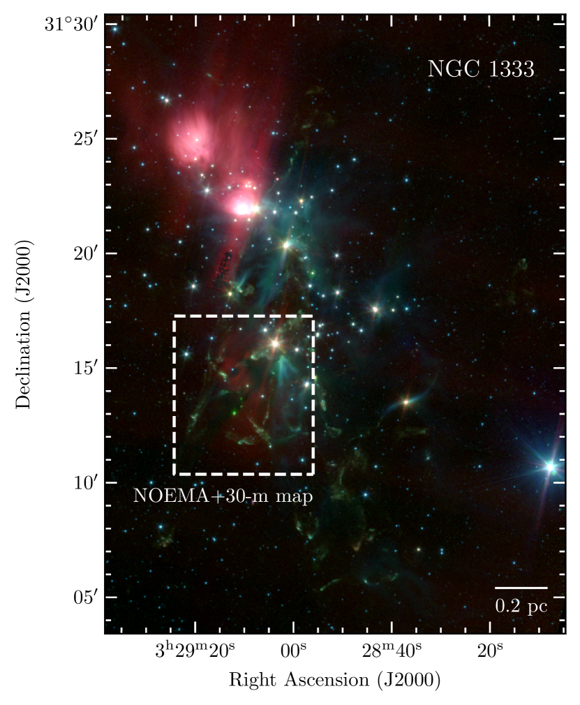
Figure 1: Color image of the NGC 1333 region using Spitzer IRAC 3.6, 4.5, and 8.0 $\mu$m. The image highlights the presence of outflows in a green color. The area covered by the combined NOEMA and 30-m observations is shown with the dashed box. The scale bar is shown in the bottom-right corner.

2.1 IRAM 30-m telescope

The observations were carried out with the IRAM 30-m telescope at Pico Veleta (Spain) on 2021 November 9, 10, and 11 and on 2022 February 19 and 20 under project 091-21. The EMIR E090 receiver and the FTS50 backend were employed. We used two spectral setups to cover the H^13CO+ (1–0) and DCO+ (1–0) lines at 72.0 and 86.7 GHz (see Table 1). We mapped a region of $\approx$150″$\times$150″with the On-the-Fly mapping technique and using position switching. The data reduction was performed using the CLASS program of the GILDAS package. The beam efficiency, $B_{eff}$, was obtained using the Ruze formula (available in CLASS), and it was used to convert the observations into main beam temperatures, $T_{\rm mb}$. The noise for the H^13CO+ (1–0) and DCO+ (1–0) cubes is 48 and 79 mK, in $T_{\rm mb}$ scale, respectively.

2.2 NOEMA interferometer

The observations carried out with the IRAM NOrthern Extended Millimeter Array (NOEMA) interferometer within the S21AD program using the Band 1 receiver were obtained on 2021 July 18, 19, and 21; August 10, 14, 15, 19, 22, and 29; and September 1 in the D configuration. We observed a total of 96 pointings, which were separated into four different scheduling blocks. The mosaic’s center is located at $\alpha_{J2000}$=03^h29^m10.2^s, $\delta_{J2000}$=31 $\degr$13$\arcmin$49.4$\arcsec$. We used the PolyFix correlator with a LO frequency of 82.505 GHz and an instantaneous bandwidth of 31 GHz spread over two sidebands (upper and lower) and two polarizations. The centers of the two 7.744 GHz-wide sidebands were separated by 15.488 GHz. Each sideband is composed of two adjacent basebands of $\sim$3.9 GHz width (inner and outer basebands). In total, there are thus eight basebands that were fed into the correlator. The spectral resolution is 2 MHz throughout the 15.488 GHz effective bandwidth per polarization. Additionally, a total of 112 high-resolution chunks were placed, each with a width of 64 MHz and a fixed spectral resolution of 62.5 kHz. Both polarizations (H and P) are covered with the same spectral setup, and therefore the high-resolution chunks provide 66 dual polarization spectral windows. The high spectral resolution windows used in this work are listed in Table 1.

2.3 Image combination

We resampled the original 30-m data to match the spectral setup of the NOEMA observations. We used the task uvshort to generate the pseudo-visibilities from the 30-m data for each NOEMA pointing. The imaging was done with natural weighting, a support mask, and using the SDI deconvolution algorithm.

Table 1: Lines observed in the high-spectral resolution band.

Transition	Rest Freq.	Beam	rms
	(MHz)	(″$\times$″)	(m$\rm Jy\,beam^{-1}$)
DCO+ (1–0)	72039.3122	6.2$\times$6.0(-37$\degr$)	23
H^13CO+ (1–0)	86754.2884	5.0$\times$4.9(-43$\degr$)	15

The H^13CO+ (1–0) was then convolved to match the DCO+ (1–0) beam size using the spectral-cube and RadioBeam Python packages. The noise level of the combined images is reported in Table 1. Both cubes were converted to units of K, and the integrated intensity maps were calculated between 5.4 and 10 ${\rm km\,s^{-1}}$, which covers all the emission seen in both molecules. The integrated intensity maps are shown in Fig. 2.

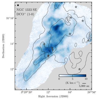
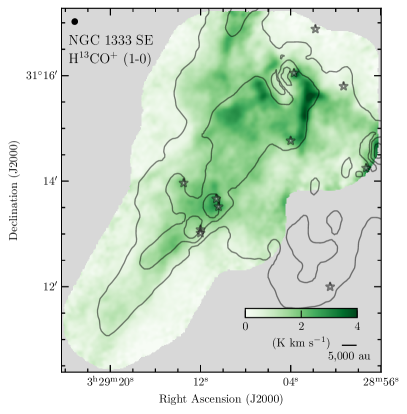
Figure 2: Maps of the DCO+ and H^13CO+ (1–0) emission obtained with NOEMA and 30-m telescopes. The beam size and scale bar are shown in the top left and bottom right, respectively. The contours correspond to the Herschel-based H2 column map; the first level is at $\log_{10}(N(\ce{H2}))=22.2$, and the step between levels is 0.5 dex. The stars mark the positions of the YSOs identified by Dunham et al. (2015) using Spitzer observations.

2.4 H2 column density

We used the total H2 column density, $N(\ce{H2})$, derived using the Herschel observations (Pezzuto et al., 2021), which are available in the Herschel Gould Belt Survey repository. The effective angular resolution of the $N(\ce{H2})$ maps is 18.2″. The map was regridded to match the DCO+ integrated intensity map. The resulting map is shown in Fig. 3.

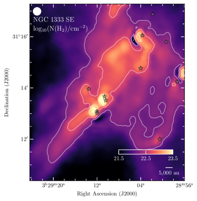
Figure 3: Map of the Herschel-based H2 column map, $N(\ce{H2})$. The contours are drawn starting at $\log_{10}(N(\ce{H2}))=22.2$ and with a step between levels of 0.5 dex. These contours are the same as in Fig. 2. The beam size and scale bar are shown in the top left and bottom right, respectively.

2.5 JCMT C^18O observations

We used the C^18O (3–2) observations of NGC 1333 taken with HARPS at JCMT (Curtis et al., 2010). The angular resolution of these observations is 17.7″, and the main beam efficiency is 0.66 (as used in Curtis et al., 2010). We smoothed the C^18O data to match the angular resolution of the Herschel-based $N(\ce{H2})$. The integrated intensity map we calculated is between 6 and 10 ${\rm km\,s^{-1}}$. This range covers all the emission seen in the cube.

Figure 4: Integrated intensity map of the C^18O (3–2) transition line. The contours correspond to the Herschel-based H2 column map, with the same contours as in Fig. 2. The beam size and scale bar are shown in top left and bottom right, respectively.

3 Analysis

3.1 Estimate of ionization fraction and cosmic-ray ionization rate

One of the most commonly used ionization fraction tracers is [DCO+]/[HCO+] (Guelin et al., 1977, 1982; Dalgarno & Lepp, 1984; Caselli et al., 1998). We estimated the ionization fraction, $X(e)$, and the cosmic-ray ionization rate, $\zeta(\ce{H2})$, following Caselli et al. (1998). The method uses the main reaction paths for the formation and destruction for HCO+ and DCO+. Although other line ratios and techniques have been explored (Bron et al., 2021), we used a method that combines the bright lines available in the observations and the CO depletion. The analysis relations between the observables and the desired physical parameters are

$$X(e) = \frac{2.7\times 10^{-8}}{R_{\rm D}}-\frac{1.2\times 10^{-6}}{f_{D}}\leavevmode\nobreak\ ,$$ (1)

$$\zeta(\ce{H2}) = \left[7.5\times 10^{-4}X(e)+\frac{4.6\times 10^{-10}}{f_{D}}\right]X(e)\,n(\ce{H_{2}})\,R_{\rm H}\leavevmode\nobreak\ ,$$ (2)

where $R_{\rm D}\equiv[\ce{DCO+}]/[\ce{HCO+}]$; $f_{D}\equiv[\ce{{}^{12}CO}]/[\ce{H2}]/\left([\ce{{}^{12}CO}]/[\ce{H2}]\right)_{\rm fiducial}$; $\left([\ce{{}^{12}CO}]/[\ce{H2}]\right)_{\rm fiducial}$ is the expected ^12CO abundance; $R_{\rm H}\equiv[\ce{HCO+}]/[\ce{{}^{12}CO}]$; and $n(\ce{H2})$ is the average H2 number density.

However, since HCO+ is usually optically thick and it also traces outflow emission (not traced by DCO+), we used H^13CO+ and the canonical isotropic ratio of $[\ce{{}^{12}C}]/[\ce{{}^{13}C}]=68$ (Milam et al., 2005) to derive $R_{\rm D}$. Similarly, we used C^18O and the canonical isotropic ratio of $[\ce{{}^{12}CO}]/[\ce{C^{18}O}]=560$ (Wilson & Rood, 1994) to estimate the ^12CO column density.

3.2 Column densities

3.2.1 DCO+ and H^13CO+

We used the optically thin approximation to derive the column densities (Mangum & Shirley, 2015). In this case, we used the following expression to calculate the total column densities:

$$N_{\rm tot}=\frac{8\pi\,\nu^{3}}{c^{3}}\frac{Q(T_{\rm ex})}{A_{\rm ul}g_{\rm u}\,e^{-E_{\rm up}/h\,T_{\rm ex}}}\frac{1}{\left(e^{h\nu/k_{B}T_{\rm ex}}-1\right)}\frac{\int T_{\rm mb}dv}{J(T_{\rm ex})-J(T_{\rm bg})}\leavevmode\nobreak\ ,$$ (3)

where $\nu$ is the frequency of the transition observed, $A_{ul}$ is the Einstein coefficient for the transition from level $u$ to $l$, $g_{\rm u}$ is the degeneracy of level $u$, $E_{\rm up}$ is the energy of level $u$, $T_{\rm ex}$ is the excitation temperature, $Q(T)$ is the partition function at temperature $T$, and $J(T)\equiv h\nu/k_{B}\,(\exp(h\nu/k_{B}\,T)-1)$ is the Rayleigh-Jeans equivalent temperature. We used the $A_{\rm ul}$, $g_{\rm u}$, and $E_{\rm up}$ listed in the LAMDA database, and implemented in the molecular_columns package.

In this work, we used a constant excitation temperature of 10 K for both transitions. Moreover, we only used estimates of the column density toward pixels with a signal-to-noise ratio of the line above 7.5 ($T_{\rm peak}>7.5\times rms$) in order to obtain robust column densities.

3.2.2 C^18O

The C^18O column density was derived using the optically thin approximation,

$$N(\ce{C^{18}O})=5\times 10^{12}\,\frac{T_{\rm ex}}{\rm K}\,\exp{(31.6\,{\rm K}/T_{\rm ex})}\,\frac{\int T_{\rm mb}{\rm d}v}{{{\rm km\,s^{-1}}}}\leavevmode\nobreak\ {\rm cm^{-2}}\leavevmode\nobreak\ ,$$ (4)

and an excitation temperature of $T_{\rm ex}=$12 K, which were previously used by Curtis et al. (2010). These excitation temperature values are similar to those derived using ^12CO (1–0) but with lower angular resolution in this region (Pineda et al., 2008). We also estimated the optical depth in the map for the assumed $T_{\rm ex}$ and obtained a typical value of $\sim$0.4, which suggests that the optical depth is not an issue across the map. However, it might produce lower limits to the derived $N(\ce{C^{18}O})$. Appendix A shows details regarding the optical depth calculation and a figure showing the map.

3.3 CO depletion factor

We estimated the CO depletion factor, $f_{D}$, using the C^18O column density, $N(\ce{C^{18}O})$, the isotopologue abundance ratio of $\ce{{}^{12}CO}/\ce{C^{18}O}=560$ (Wilson & Rood, 1994), the H2 column density derived from Herschel, and the expected $[\ce{{}^{12}CO}]/[\ce{H2}]=2.7\times 10^{-4}$ value, as determined in Taurus (Punanova et al., 2022) and comparable to the value of $2.5\times 10^{-4}$ obtained in NGC1333 at a lower angular resolution (Pineda et al., 2008). When comparing the $N(\ce{H2})$ and $N(\ce{C^{18}O})$ column densities maps, it was clear that the H2 map traces more extended emission, and therefore, an offset is present,

$$N(\ce{H2})=N(\ce{C^{18}O})\frac{[\ce{H2}]}{[\ce{C^{18}O}]}+\delta_{18}\leavevmode\nobreak\ .$$ (5)

This offset represents the H2 column in the molecular cloud that is not traced by the C^18O (3–2) emission, and therefore it needed to be removed from the abundance calculations. We estimated the offset, $\delta_{18}=2.7\times 10^{21}$ cm^-2, as the median value of the difference observed assuming an undepleted abundance in the column density range of $3\times 10^{21}\,{\rm cm^{-2}}<N(\ce{H2})<5\times 10^{21}\,{\rm cm^{-2}}$. This is equivalent to determining the offset required to achieve undepleted abundances at the lower column densities in the region. The resulting map is shown in Fig. 5, with depletion fractions increasing at higher column densities.

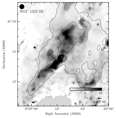
Figure 5: Map of the CO depletion fraction, $f_{D}$. The beam size and scale bar are shown in the top-left and bottom-right corners, respectively. The contours correspond to the Herschel-based H2 column map; the contours are the same as in Fig. 2.

3.4 Volume density

We estimated the volume density as

$$n(\ce{H2})=\frac{N(\ce{H2})-\delta_{18}}{\delta L}\leavevmode\nobreak\ ,$$ (6)

where the $N(\ce{H2})$ is the H2 column density, $\delta_{18}$ is the derived offset with C^18O , and $\delta L$ is the depth of the structure. We assumed $\delta L=0.4$ pc ($\sim 60\times 10^{3}$ au), which is the depth for HCO+ derived for the nearby L1451 (Storm et al., 2016). The corresponding volume density map is shown in Fig. 6, and it displays densities similar to those constrained from ^12CO and ^13CO (1–0) observations (Pineda et al., 2008). The typical density in places with a detection of DCO+ and H^13CO+ is $\approx 4\times 10^{3}$ $\rm cm^{-3}$, which suggests that this density is likely a lower limit since this region is bright in NH3 (Friesen et al., 2017; Dhabal et al., 2019) and N2H+ (Hacar et al., 2017), which are reliable high-density tracers.

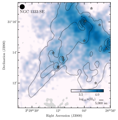
Figure 6: Volume density map estimated from Herschel H2 column density. The beam size and scale bar are shown in the top left and bottom right, respectively. The contours correspond to the Herschel-based H2 column map; the contours are the same as in Fig. 2.

3.5 Electron fraction

We used the relation of Eq. (1) together with the previously presented measurements to estimate the electron fraction across the active star-forming region, and it is presented in the left panel of Fig. 7. The underlying distribution of the electron fraction in the region was estimated using the kernel density estimate (KDE), and it is shown in the right panel of Fig. 7. A typical value (median of the $\log_{10}$) of $\langle X(e)\rangle=10^{-6.5}$ was derived from these measurements. We estimate that the error associated with using the wrong excitation temperature (in the range of 5 to 30 K) in the column density determination yields an uncertainty of less than 10% in $R_{D}$ and $X(e)$.

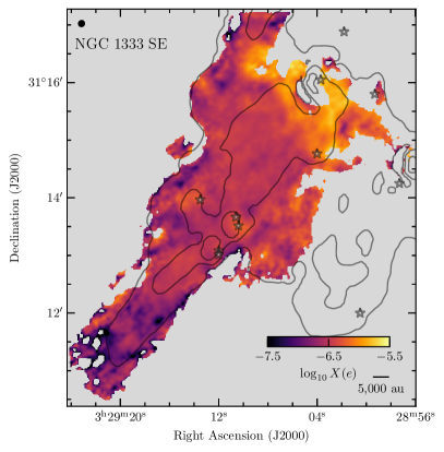
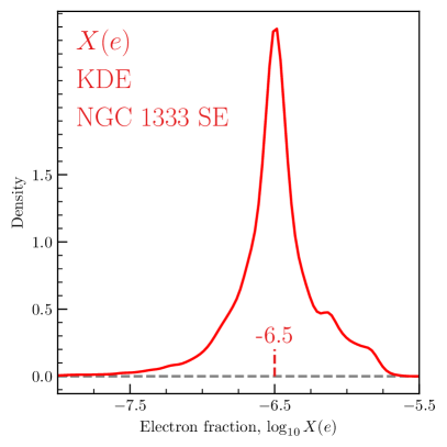
Figure 7: Derived electron fraction in the region. Left: Map of the electron fraction, $X(e)$. The map shows a smooth distribution but with a clear enhancement in the northwest section. The beam size and scale bar are shown in the top left and bottom right, respectively. The contours correspond to the Herschel-based H2 column map; the contours are the same as in Fig. 2. Right: Kernel density estimate of the $X(e)$ distribution across the mapped region. A typical value (median of the $\log_{10}$) of $10^{-6.5}$ was derived from these measurements and is marked with a red dashed vertical line.

3.6 Cosmic-ray ionization rate

We used the relation of Eq. (2) together with the previously presented measurements to estimate the cosmic-ray ionization rate across the active star-forming region, and the estimate is presented in the left panel of Fig. 8. The underlying distribution of the cosmic-ray ionization rate in the region was estimated using the KDE, and it is shown in the right panel of Fig. 8. We derived a typical value (median of the $\log_{10}$) of $\langle\zeta(\ce{H2})\rangle=10^{-16.3}$ s^-1 from these measurements. We estimate that the error associated with using the wrong excitation temperature (with the temperature within the range of 5 and 30 K) $R_{H}$ could be underestimated by up to a factor of two, in addition to the uncertainty of less than 10% in $R_{D}$ and $X(e)$ mentioned in Sect. 3.5. This indicates that the $\zeta(\ce{H2})$ could be underestimated by a factor of two toward hot regions ($T_{ex}>20$K), but elsewhere, these uncertainties are of the order 10–30%.

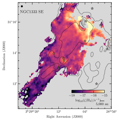
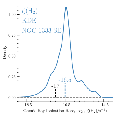
Figure 8: Derived cosmic-ray ionization rate in the region. Left: Map of the cosmic-ray ionization rate, $\zeta(\ce{H2})$. The map shows a smooth distribution but with the value clearly increasing in the northwest section. The beam size and scale bar are shown in top left and bottom right, respectively. The contours correspond to the Herschel-based H2 column map; the contours are the same as in Fig. 2. Right: Kernel density estimate of the $\zeta(\ce{H2})$ distribution across the mapped region. The median value of the $\log_{10}\zeta(\ce{H2})/{\rm s}^{-1}=-16.5$ and the canonical value of $10^{-17}$ s^-1 are marked with the blue and black dashed vertical lines, respectively.

4 Discussion

4.1 Electron fraction and cosmic-ray ionization rate distributions

The spatial distribution for both of the main parameters estimated in this work, $X(e)$ and $\zeta(\ce{H2})$, are shown in the left panel of Figs. 7 and 8. These maps show the first resolved maps of these quantities, which present little substructure, except close to the cloud or structure’s edge and close to the young protostars. These maps were derived at the angular resolution of the DCO+ map, but we note that since $n(\ce{H2})$ and $f_{D}$ were derived using Herschel data, we assumed that they smoothly vary between 16$\arcsec$ and $\approx$6$\arcsec$, which might be less accurate toward the young protostars.

4.2 Electron fraction as a function of density

Several attempts have been carried out to parametrize the variation of the electron fraction as a function of density. McKee (1989) presented an analytic relation for the electron fraction as a function of density assuming no depletion of metals and a constant cosmic-ray ionization rate. This relation is expected to work even at high densities (McKee & Ostriker, 2007). After the depletion of metals was identified as an important process in the denser regions within star-forming regions, an updated electron fraction relation with the density relation was presented by Caselli et al. (2002b), where a constant cosmic-ray ionization rate was assumed. Further detailed modeling of the prestellar core L1544 using different molecular transitions constrained the radial profile electron fraction (Redaelli et al., 2021). This derived relation is closer to that derived by Caselli et al. (1998), while (McKee, 1989) provides a clear overestimation.

We compared the KDE distribution of the values determined from the data and the analytic relations in Fig. 9. In addition, we added a comparison with the relation obtained from modeling the L1544 prestellar core (Redaelli et al., 2021). A decrease in the electron fraction, $X(e)$, at higher densities, $n(\ce{H2})$, is a common trend from the analytical (and modeling) results. Notably, Fig. 9 shows a consistent increase in the electron fraction toward higher density areas, while beyond $n(\ce{H2})\gtrsim 10^{3.7}$ $\rm cm^{-3}$, the relation steepens. This steeper relation is mostly driven by the northwest area in the map, which is coincident with a previously suggested bubble interacting with the cloud (e.g., Dhabal et al., 2019; De Simone et al., 2022).

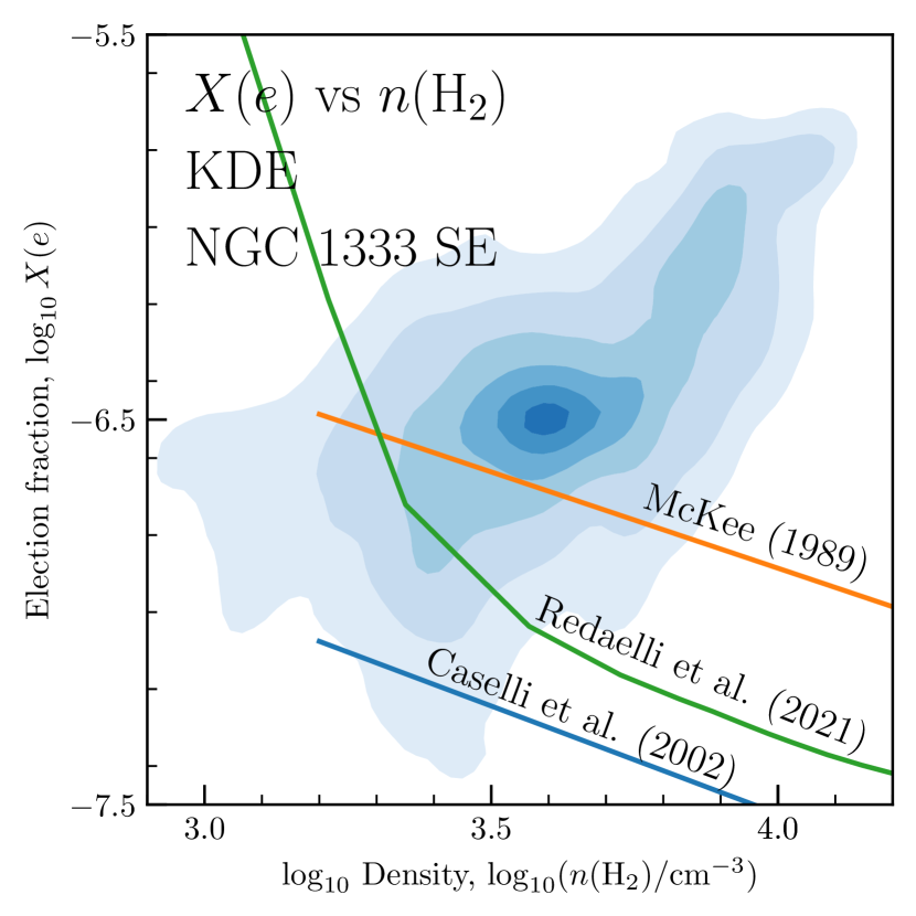
Figure 9: Electron fraction, $X(e)$, as a function of H2 density. The KDE of the underlying distribution was obtained from the data. The contour levels are drawn starting at 0.5$\sigma$ and progressing outward in steps of 0.5$\sigma$, where the $\sigma$ levels are equivalent to that of a bivariate normal distribution. The analytic relations from McKee (1989) and Caselli et al. (2002b) as well as the result from chemical modeling of L1544 (Redaelli et al., 2021) are shown with orange, blue, and green curves, respectively. The analytic relations shown here do not take into account the local generation of cosmic rays.

A key difference between the analytical relations for electron fraction as a function of density and data is the assumption of no local sources of cosmic rays. Recently, different works have suggested that enhanced levels of cosmic rays (thanks to their local generation by YSOs, e.g., Ceccarelli et al., 2014; Padovani et al., 2016) could provide a higher value of electrons than previously expected. This important difference might be the main physical reason as to why the analytical relations have such a poor match to the data, even in the case of McKee (1989), who reported a similar predicted value at the typical density ($\approx 10^{3.7}$ $\rm cm^{-3}$) even though there is a clear measurement of the depletion of metals ($f_{D}$).

The derived densities are comparable to previous estimates. The mean density in the region probed with ^12CO and ^13CO (1–0) transitions are $\approx 10^{3}$ $\rm cm^{-3}$ (Pineda et al., 2008). Therefore, although our density estimate is rather simple and likely a lower limit, it should not be the main reason for the disagreement between the measured electron fractions and the theoretical models.

4.3 Local generation of cosmic rays

Recently, several indirect observations have suggested an extremely high ionization rate over $10^{-15}$ s^-1 in protostellar environments (e.g., Ceccarelli et al., 2014; Fontani et al., 2017; Favre et al., 2018; Cabedo et al., 2023). Also, synchrotron emission, the fingerprint of the presence of relativistic electrons, has been detected in the shocks that develop along protostellar jets (e.g., Beltrán et al., 2016; Rodríguez-Kamenetzky et al., 2017; Osorio et al., 2017; Sanna et al., 2019). Neither signature can be explained by interstellar cosmic rays since they are strongly attenuated at the high column densities typical of protostellar environments. As argued by Padovani et al. (2016) and Padovani et al. (2021), shocks forming along the jets and on the protostellar surface could be the regions where the locally accelerated cosmic rays are produced.

The left panel of Fig. 8 shows a dramatic local increase of $\zeta(\ce{H2})$ occurring in the northwest (upper) section of the map. Furthermore, there is a noticeable enhancement of $\zeta(\ce{H2})$ when in proximity to the embedded YSOs, which are also in the central area of the studied region. In fact, the volume density in dense cores around YSOs (typically within $\lesssim$0.1 pc, Kirk et al. 2006) is much higher than the ”large-scale” estimate based on Eq. (6). Therefore, according to Eq. (2), the actual value of $\zeta(\ce{H2})$ is expected to be further drastically enhanced around these YSOs. In order to gain insights into the underlying mechanisms of the observed phenomenon, in Fig. 10, we have overlaid the cosmic-ray ionization rate map with the outflow orientation of the different embedded sources (see Table 2), the dust polarization vectors obtained from the JCMT SCUBA2-POL Bistro Survey (Ward-Thompson et al., 2017) on this region (Doi et al., 2020, 2021), and the X-ray sources detected with Chandra (Winston et al., 2010).

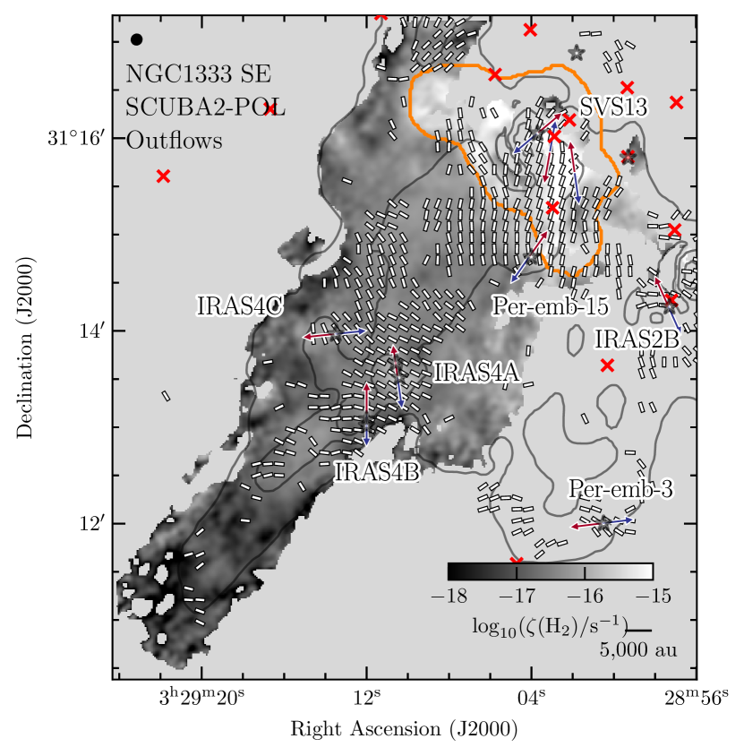
Figure 10: Outflows and magnetic field orientation over $\zeta(\ce{H2})$. The background image is the derived $\zeta(\ce{H2})$ map, as shown in Fig. 8. The region identified with a local cosmic-ray ionization rate enhancement is marked with an orange contour. The outflow lobes (as reported in previous works) are shown by red and blue arrows. The magnetic field orientation, measured from continuum polarization observations with SCUBA2-POL, are shown by the segments of white lines. The X-ray sources are marked with red crosses. The beam size and scale bar are shown in the top-let and bottom-right corners, respectively.

First, we ruled out the X-ray sources as a possible explanation of the observed ionization enhancement. A significant attenuation of X-ray photons produced by source emitting in the keV energy range starts at column densities of $\sim 10^{23}$ cm^-2 (Igea & Glassgold, 1999), which is about the measured maximum value of $N(\ce{H2})$ in the upper section (where most of the sources are located). Therefore, X-rays would result in a relatively isotropically enhanced $\zeta(\ce{H2})$ around the sources, which is clearly incompatible with the distribution of $\zeta(\ce{H2})$ seen in this region, revealing no correlation with the source locations.

However, we have strong indicators that the sources of the ionization enhancement are the young embedded objects. The first obvious fact is the noticeable increase of $\zeta(\ce{H2})$ around most of the YSOs. Given that we strongly underestimated the gas density in the proximity to these objects, the actual values of $\zeta(\ce{H2})$ are expected to be much higher than those shown in Fig. 8. Second, the elongated region with the highest local ionization rate of $\gtrsim 10^{-15}$ s^-1 in the upper section of the map is approximately parallel to the magnetic field lines, practically connecting the SVS13 system and Per-emb-15. If these objects are able to generate energetic charged particles, their further propagation and the resulting ionization must occur along the local field lines (Fitz Axen et al., 2021). We note that in this work, we also include a figure of the difference between the observed CRIR and the expected values (Padovani et al., 2018) in Appendix C, which shows the same trends.

We compared the CRIR as a function of the typical YSO distance, calculated as the harmonic mean of the individual distances,

$$\frac{1}{d_{YSO}^{2}}=\frac{1}{N}\sum_{i=1}^{N}\frac{1}{d_{i}^{2}}\leavevmode\nobreak\ ,$$

where $d_{i}$ is the distance to the different YSOs marked in Fig. 10. Figure 11 shows the KDE for the map, and it shows that within 15,000 au, the CRIR is relatively constant, while there is a reduction in the CRIR at larger distances. This is evidence that the YSOs are related to the increase of the CRIR. Although, we cannot confirm a correlation between YSO luminosity and CRIR due to the small sample size and the issues determining accurate CRIR toward the YSOs.

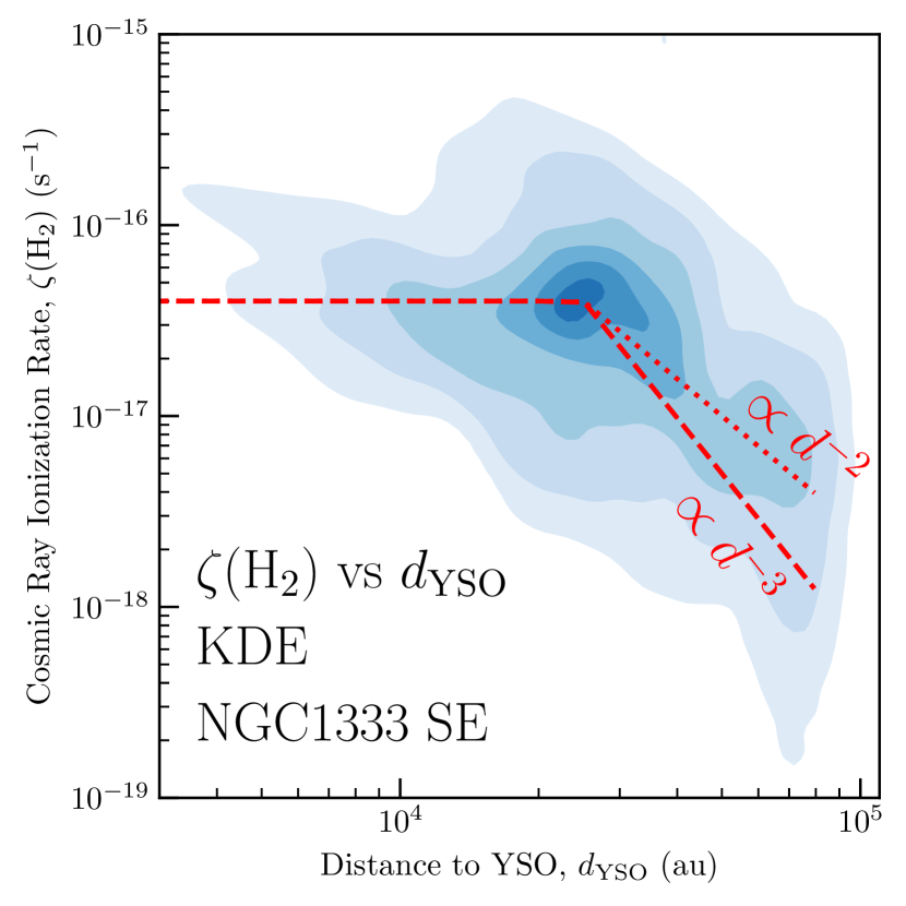
Figure 11: Cosmic-ray ionization rate as a function of distance to YSOs. The KDE of the CRIR and the typical distance to the YSOs, $d_{YSO}$, was calculated over the map. The dotted and dashed lines show the inner constant section, and the two different power-law decays help guide the eye.

It is worth noting that the three-color Spitzer image in Fig. 1 shows a strong outflow emission (green) from the SVS13 region, which overlaps with a fraction of the high enhancement in the cosmic-ray ionization rate. The SVS13 region hosts several strong and well-studied outflows (Maret et al., 2009; Hodapp & Chini, 2014; Lefèvre et al., 2017; Dionatos et al., 2020). It is possible that part of the local enhancement in CRIR is related to the outflow cavity, especially if we are probing the emission closer to the outflow cavity itself. Models following CR propagation indicate that the CR distribution near accelerating protostellar sources is likely inhomogeneous with the CR enhancement occurring along the direction of the outflow (Fitz Axen et al., 2021).

We would like to emphasize that most of the observed region (in particular, the lower section of the map in Fig. 8) is dominated by $\zeta(\ce{H2})\sim 10^{-17}$ s^-1. This level of ionization, likely generated by interstellar cosmic rays, is comparable to the ”standard” value of the ionization rate in diffuse molecular clouds Glassgold & Langer (1974). This value is also in good agreement with constraints on the CRIR derived from energy arguments. For the Milky Way, Krumholz et al. (2023) inferred a mean primary ionization budget due to star-formation activity of $\zeta(\ce{H2})\sim 2-5\times 10^{-17}$ s^-1, significantly below the value measured in diffuse molecular gas. These values can be reconciled if CR acceleration sources are distributed inhomogeneously.

Remarkably, we can independently estimate the expected upper bound of the ionization rate near NGC 1333 produced by interstellar cosmic rays in the surrounding diffuse gas. One of the measurements of H3+ ions reported by Indriolo & McCall (2012) was performed in the direction of the target star HD 21483. Along this line of sight, the measurements probe the cosmic-ray ionization at the same radial distance of 300 pc, which is only 4–5 pc away from NGC 1333 in the plane of sky. The resulting non-detection yields a $1\sigma$ upper limit of $9\times 10^{-17}$ s^-1 for the ionization rate. Given that the obtained spectra of H3+ lines show no visible traces of absorption (see their Fig. 10), we conclude that the actual value of $\zeta(\ce{H2})$ in this region is substantially lower and may well be close to the expected ”standard” value.

In a separate publication, we will present a detailed analysis of the ionization rate map. We will also perform a quantitative comparison of the results with available theories of propagation of interstellar and locally accelerated cosmic rays.

4.4 Evidence of shocks and interaction

The spatial distribution for both of the main parameters estimated in this work, $X(e)$ and $\zeta(\ce{H2})$, are shown in the left panel of Figs. 7 and 8. Both quantities present a clear one-order-of-magnitude enhancement toward the northwest in the mapped region. This could be consistent with the suggestion that the region is affected by interaction with an expanding shell (De Simone et al., 2022) coming from the northwest section of the map (the SVS13 region). A similar interaction, although at a much larger scale, is suggested in the nearby Taurus cloud with the Local Bubble and the Per-Tau shell (Soler et al., 2023), which could also be occurring in the Perseus Cloud.

A second region along the southwest of the map has previously been suggested as showing evidence of interaction between the cloud and a turbulent cell (Dhabal et al., 2019) or of a second bubble impacting the cloud (De Simone et al., 2022). However, we do not see clear evidence in $X(e)$ or $\zeta(\ce{H2})$ of any of these features, although we cannot rule them out.

4.5 The relevance of nonideal-MHD effects

On scales of a couple of beams away from the embedded sources, the ionization fraction is $\approx 10^{-6.5}$ (see Fig. 7). It is usually assumed that at a relatively high electron fraction, the nonideal-MHD terms are negligible. Studying the initial core collapse phase Wurster et al. (2018) showed that above cosmic-ray ionization rates of $\langle\zeta(\ce{H2})\rangle>10^{-14}{\rm s}^{-1}$, the results are practically indistinguishable from results obtained by assuming zero resistivity (i.e., ideal MHD). The values measured in NGC 1333 are slightly higher with respect to the often-assumed canonical value for prestellar cores of $\langle\zeta(\ce{H2})\rangle\approx 10^{-17}{\rm s}^{-1}$ (Spitzer & Tomasko, 1968; Umebayashi & Nakano, 1990), and therefore, the nonideal-MHD effects are expected to not play an important role in current and future disk formation.

4.6 MHD wave cutoff

In a molecular cloud where the ionization level is low, the Alfvé waves cannot propagate when the collision frequency between ions and neutrals is comparable to or smaller than the MHD wave frequency. Therefore, a critical length for wave propagation beyond which waves do not transmit can be defined. The critical length for wave propagation (Stahler & Palla, 2005; Mouschovias et al., 2011) is obtained from

$$\lambda_{min}=\sqrt{\frac{\pi}{4\mu\,m_{\ce{H}}\,n(\ce{H2})}}\frac{B_{o}}{n(\ce{H2})\,X(e)\,\langle\sigma\,v\rangle\leavevmode\nobreak\ },$$ (7)

where $B_{o}$ is the unperturbed magnetic field and $\langle\sigma\,v\rangle$ is the rate coefficient for elastic collisions. The rate coefficient term is approximated by the Langevin term,

$$\langle\sigma\,v\rangle=1.69\times 10^{-9}\,{\rm cm^{3}\,s^{-1}}\leavevmode\nobreak\ ,$$ (8)

for HCO+–H2 collisions (McDaniel & Mason, 1973). We estimated the magnetic field strength, $B_{o}$, using the relation of Crutcher et al. (2010), a typical volume density of $10^{3.6}$ $\rm cm^{-3}$, and the median value of $X(\ce{e})=10^{-6.5}$. With these values, we then obtained an MHD wave cutoff scale of 0.054 pc (11 100 au). Therefore, we predicted that if the turbulence is MHD in nature, then a dissipation scale should be observed at $\approx$0.054 pc (or $\approx$37$\arcsec$ at the distance of Perseus).

Previously, this scale was proposed as a possible origin for the transition to coherence between the supersonic cloud and subsonic cores ($\sim$0.1 pc; Goodman et al., 1998; Caselli et al., 2002a; Pineda et al., 2010). Recent observations of dense gas with different tracers (e.g., N2H+ and NH3) and angular resolutions showed that the southern end filament presents subsonic levels of turbulence at scales of $\approx$40$\arcsec$ (Friesen et al., 2017; Hacar et al., 2017; Dhabal et al., 2019; Sokolov et al., 2020), which corresponds to 0.054 pc, or 11 200 au, at the distance of Perseus. This is consistent with the estimated dissipation scale; however, studies of turbulence at higher angular resolution than 30″should reveal this scale.

4.7 Disk sizes

Of the 12 Class 0 and I protostars in this region, dust emission observations of disks have resolved only six sources with either VLA or ALMA continuum observations (Segura-Cox et al., 2016, 2018; Diaz-Rodriguez et al., 2022). The mean dust disk radii measured for these six resolved sources is $\approx$30 au (see Table 2). These values are lower than the typical values obtained for Class 0 and I objects (median values of 61 au and 81 au for Class 0 and I, respectively; see Tsukamoto et al., 2023, for a recent review).

Theoretical models suggest disk properties are sensitive to the degree of coupling between ions and neutrals, with perfect coupling corresponding to the ”ideal” MHD limit in which angular momentum is efficiently transported away from the circumstellar region by magnetic braking (Zhao et al., 2020). Higher levels of CR ionization effectively enhance magnetic braking, thereby leading to smaller disks (Dapp et al., 2012; Zhao et al., 2016; Wurster et al., 2016). For example, Kuffmeier et al. (2020) carried out a suite of simulations that followed the collapse of spherical cores and showed that the disk size decreases with an increasing cosmic-ray ionization rate for identical initial conditions because of more efficient magnetic braking. Although prestellar cores appear as more dynamic entities in larger scale simulations (Kuffmeier et al., 2017; Lebreuilly et al., 2021; Offner et al., 2022), the results from Kuffmeier et al. (2020) provide a well-controlled experiment with different mass-to-flux-ratios

$$\lambda_{mag}\equiv\frac{M_{\rm c}}{\pi R_{\rm c}^{2}B_{0}}2\pi\sqrt{G}\leavevmode\nobreak\ ,$$ (9)

where $B_{0}$ is the magnetic field strength, and $M_{\rm c}$ and $R_{\rm c}$ are the mass and radius of the core.

For the typical values of the ionization and cosmic rays found in this work, $\langle X(e)\rangle=10^{-6.5}$ and $\langle\zeta(\ce{H2})\rangle=10^{-16.5}$ s^-1 = $3\times 10^{-17}$ s^-1, the typical gas disk sizes found in this region are well matched by the cases in Kuffmeier et al. (2020) with $\lambda_{mag}=5$ and an initial ratio of rotational to gravitational energy, $\beta$, of the spherical core between $\beta=0.025$ and $\beta=0.1$ (see also Wurster et al. (2018)). Similarly, Lebreuilly et al. (2021) investigated the disk size distribution in nonideal-MHD models, assuming an ionization rate of $\langle\zeta(\ce{H2})\rangle=10^{-17}$ s^-1, of a collapsing clump of 1 000 $\rm M_{\odot}$. They found an average disk radius of $\approx$50 au, which is about a factor of two larger than what is found in our observations. This might indicate that the relatively higher cosmic-ray ionization rate in NGC 1333 leads to smaller disk sizes, although a lower angular momentum or higher magnetization cannot be ruled out.

We highlight that the cosmic-ray ionization rate is not a constant value throughout the entire region, and it may fluctuate, especially toward higher densities closer to the actively accreting protostars. At these high densities, this rate could decrease due to the shielding of cosmic rays (Nakano & Tademaru, 1972; Umebayashi & Nakano, 1981; Padovani et al., 2009), or it could increase due to local enhancement of cosmic-ray ionization by the individual protostars themselves (Padovani et al., 2016; Gaches & Offner, 2018).

4.8 Improvements on $X(e)$ and $\zeta(\ce{H2})$

Although the method for determining the electron fraction and cosmic-ray ionization rate is widely used, there are clear paths for improvements. The assumption of a single excitation temperature could impact the total column densities derived and the derived $X(e)$ and $\zeta(\ce{H2})$. However, the H^13CO+ and DCO+ (1–0) lines have similar parameters ($E_{up}$ and $A_{ul}$), and therefore, this assumption is not expected to cause major issues. Also, other transitions of these species, combined with an excitation analysis, could better constrain the optical depth and excitation temperatures of these species and therefore derive more reliable molecular column densities.

Recently, Sabatini et al. (2023) has shown that in high-mass star-forming regions, where DCO+ and H^13CO+ might trace different volumes or be affected by high optical depths, H2D+ is a better estimator for the cosmic-ray ionization rate. Unfortunately, this approach is severely limited in low-mass star-forming regions since the H2D+ emission is compact and only traces the highest density regions in dense cores (e.g., Caselli et al., 2003; van der Tak et al., 2005; Harju et al., 2006; Vastel et al., 2006; Caselli et al., 2008; Friesen et al., 2010, 2014; Koumpia et al., 2020).

A complementary approach might involve analyzing multiple molecular species and/or transitions and comparing the line emission with a suite of chemical models to directly constrain the typical physical parameters of the region (e.g., density, radiation field, $\zeta(\ce{H2})$, ”chemical” age). This could be carried out with single-zone models (0D) or more complex ones using some physical model for the region. Regardless of the approach, a new and exciting possibility of deriving robust and high-quality resolved maps of $X(e)$ and $\zeta(\ce{H2})$ is upon us.

5 Conclusions

We have presented the first results of the ProPStar survey. We studied the southeast section of the NGC 1333 region using combined observations of the 30-m and NOEMA telescopes to recover all scales. The main results are listed below:

1. We mapped the DCO+ and H^13CO+ (1–0) emission at $\approx 6\arcsec$ resolution ($\approx$1 800 au).

2. We used the analytic relation from Caselli et al. (1998) relating the measured DCO+ and H^13CO+ column density ratio in addition to archival C^18O and H2 in order to derive the first large-area map for the electron fraction, $X(e)$, and cosmic-ray ionization rate, $\zeta(\ce{H2})$, in a low-mass star-forming region.

3. The electron fraction and cosmic-ray ionization rate distributions are peaked at about $10^{-6.5}$ and $10^{-16.5}$ s^-1, respectively, showing local enhancements around the embedded YSOs. These values are higher than expected from the ”standard” cosmic-ray ionization rate in molecular clouds.

4. The northwest region in the map shows highly elevated values for both the electron fraction and cosmic-ray ionization rate, which might be a sign of the interaction between the molecular cloud and a local bubble, or it could be due to cosmic rays being locally generated by YSOs.

5. We used the typical value of $X(e)$ in the region to estimate the critical length for wave propagation of MHD turbulence of 0.054 pc ($\approx$37″). If the turbulence in the molecular clouds is of MHD nature, then this dissipation scale could be measured with observations of enough sensitivity and resolution.

6. The increased values of $X(e)$ and $\zeta(\ce{H2})$ are sufficiently high such that when compared to numerical simulations, the newly formed disks should be consistent with ideal-MHD simulations (e.g., small). This also suggests that disk formation in clustered regions could strongly depend on the feedback from the first stars that are formed.

In summary, these observations show the great potential offered by combined NOEMA and IRAM 30-m observations to determine the electron fraction and cosmic-ray ionization rate in the NGC 1333 region. Both of these quantities are important to understanding the physical conditions and processes involved in star and disk formation. More maps of the cosmic-ray ionization rate and electron fraction, combined with complementary disk size measurements, should provide a much better understanding of the role of stellar feedback (e.g., locally generated cosmic rays) and the importance of nonideal MHD in the whole star- and disk-formation processes.

Appendix A Optical depth of C^18O

We estimated the C^18O (3–2) line optical depth as

$$\tau(\ce{C^{18}O})=-\ln\left(1.0-\frac{T_{p}(\ce{C^{18}O})}{J_{\nu}(T_{ex})-J_{\nu}(T_{cmb})}\right)\leavevmode\nobreak\ ,$$ (10)

where $T_{p}(\ce{C^{18}O})$ is the peak brightness of the line, and $J_{\nu}(T)$ is the brightness temperature of a black body with temperature $T$ at frequency $\nu$. In the case of C^18O (3–2), we assumed $T_{ex}=12$ K.

Figure 12 shows the map of the optical depth. The figure clearly shows that the emission is mostly optically thin, which is also consistent with the findings from Curtis et al. (2010).

Figure 12: Optical depth of C^18O (3–2). The red line shows the $\tau(\ce{C^{18}O})=1$ contour. The contours correspond to the Herschel-based H2 column map; the contours are the same as in Fig. 2. The beam size and scale bar are shown in the top-let and bottom-right corners, respectively.

Appendix B The effect of excitation temperature

One of the most important simplifications in this work was the use of a single excitation temperature for the column density calculation of H^13CO+ and DCO+, which we used to determine the $R_{\rm D}$ and $R_{\rm H}$ quantities. We explored the effect of both species having the same excitation temperature but that temperature being different from 10 K (5 K $<T_{\rm ex}<$ 12 K), and we found that the variation in $R_{\rm D}$ is less than $5\%$, while for $R_{\rm H}$, the variation is less than $10\%$. Therefore, an improved excitation analysis of both species would provide a substantial check to the calculation used in this work.

Appendix C $\Delta\log_{10}\zeta$

We calculated the difference between the derived CRIR and the expected values from the $\mathcal{L}$ model of CRIR as a function of column density from Padovani et al. (2018), $\Delta\log_{10}\zeta=\log_{10}\zeta_{obs}-\log_{10}\zeta_{model}$. Figure 13 shows the map of $\Delta\log_{10}\zeta$, which is similar to Fig. 8, with lower values than expected in the southeast section, local increases toward YSOs, and a general excess in the rest of the map.

Figure 13: Difference between observed CRIR and the model-$\mathcal{L}$ to better illustrate the local effects, $\Delta\log_{10}\zeta=\log_{10}\zeta_{obs}-\log_{10}\zeta_{model}$. The red and blue colors show the excess and deficiency of CRIR with respect to the expected value following Padovani et al. (2018). The contours correspond to the Herschel-based H2 column map; the contours are the same as in Fig. 2. The beam size and scale bar are shown in the top-let and bottom-right corners, respectively.

Appendix D Disk sizes and outflow directions of covered YSOs

We list the source name, disk radii, and outflow directions found in the literature in Table 2. Except for SVS13 VLA4A and SVS13 VLA4B, the disk sizes are the result of modeling VLA 8.1 mm continuum observations, which have a FWHM beam size of $\sim$16 au (Segura-Cox et al. 2016, 2018). For sources without a reported disk radii, the disks were detected but unresolved in Segura-Cox et al. (2018), and the disk radii at VLA wavelengths could only be estimated as being less than or equal to 8 au. For SVS13 VLA4A and SVS13 VLA4B, which form a close binary that shares dusty circumbinary material, the dust disk radii of the individual circumstellar disks are reported from Gaussian fits to ALMA 0.9 mm continuum observations, with a FWHM beam size of $\sim$26 au (Diaz-Rodriguez et al. 2022).

Table 2: Properties of Class 0 and I protostars within the field of view.

Source	Class	$R_{disk}$	PAoutflow	Other Name	Ref.
		(au)	(deg)
NGC 1333 IRAS4A1	0	49.7	19.2	Per-emb-12	(1, 5)
NGC 1333 IRAS4A2	0	–	20	Per-emb-12	(1, 7)
NGC 1333 IRAS4B	0	–	176	Per-emb-13	(1, 2, 5)
NGC 1333 IRAS4B2	0	–	76	Per-emb-13	(1, 8)
NGC 1333 IRAS2B	I	–	24	Per-emb-36	(1, 9)
NGC 1333 IRAS4C	0	37.2	96	Per-emb-14	(2, 6)
SVS13 VLA4A	0/I	12	8	SVS13A, Per-emb-44	(3, 4)
SVS13 VLA4B	0/I	9	-50	SVS13A, Per-emb-44	(3, 4)
SVS13 VLA17	0	31.7	170	SVS13B	(2, 5)
SVS13C	0	42.9	8	–	(1, 4)
Per-emb-15	0	–	-35	SK14	(4)
Per-emb-3	0	–	97	–	(1, 9)

(1) Segura-Cox et al. (2018), (2) Segura-Cox et al. (2016), (3) Diaz-Rodriguez et al. (2022), (4) Plunkett et al. (2013), (5) Lee et al. (2016), (6) Zhang et al. (2018), (7) Chuang et al. (2021), (8) Hull et al. (2014), (9) Stephens et al. (2017)