Extremal problems about the order and size of nonhamiltonian locally linear graphs

Abstract

The study of the relationship between local and global properties of mathematical objects has always been a key subject of investigation in different areas of mathematics. A graph $G$ is called locally linear if the neighbourhood of every vertex of $G$ induces a path. And $G$ is called locally hamiltonian (traceable) if the neighbourhood of every vertex of $G$ induces a hamiltonian (traceable) graph. The local properties of graphs are being studied extensively. For example, the minimum order of a nonhamiltonian (or nontraceable) locally hamiltonian (or traceable) graph has been determined. In this paper, we determine the minimum order of a nonhamiltonian locally linear graph and the minimum size of a nonhamiltonian locally linear graph of a given order.

2020 Mathematics Subject Classification: 05C35, 05C45, 05C69

Keywords: nonhamiltonian; locally linear graph; minimum order; minimum size

1 Introduction

We consider finite simple connected graphs, and use the standard notation throughout this article. For those not defined here, we refer the reader to Bondy and Murty [3]. The order of a graph is its number of vertices, and the size is its number of edges. We denote by $V(G)$ and $E(G)$ the vertex set and edge set of a graph $G,$ respectively. Let $S\in V(G),$ we use $G[S]$ to denote the subgraph induced by $S$. A Hamilton cycle is a cycle that contains all the vertices in $V(G)$ and a graph that contains a Hamilton cycle is called a hamiltonian graph. A Hamilton path in a graph $G$ is a path that contains all the vertices in $V(G)$, and a graph that contains a Hamilton path is called traceable.

Let $N_{G}(v)$ be the set of vertices adjacent to $v$ in $G$. When there is no danger of ambiguity, we use $N(v)$ instead of $N_{G}(v)$ for short. For a given graph property $\mathcal{P}$, we call a graph $G$ locally $\mathcal{P}$ if $G[N(v)]$ has property $\mathcal{P}$ for every vertex $v$ in $G$. For example, a graph $G$ is called locally hamiltonian if $G[N(v)]$ is hamiltonian for every vertex $v$ in $G$. The notion of local hamiltonicity was introduced by Skupień [16] in 1965. For some articles on locally hamiltonian or locally traceable, we refer to [6, 7, 4, 18]. A graph $G$ is called locally linear if $G[N(v)]$ is an induced path for every $v$ in $G$. Locally linear graphs have been studied for a long time. In 1989, Parsons and Pisanski [15] studied topological characterizations of locally linear graphs. Laskar and Mulder [11] characterized all 3-sun-free locally linear graphs in 2013. They also characterized the graphs G with $G[N(v)]=P_{k}$ for $k\leq 4$. Graphs in which the neighborhood of each vertex is some special graph are investigated in [8, 9, 12, 10, 20]

Determining the minimum order of a graph satisfying locally $\mathcal{P}$ is a classical problem in graph theory. Pareek [13] showed that the maximum degree of a non-Hamiltonian locally Hamiltonian graph is at least $8$. Furthermore, from this it follows that the minimum order of a non-Hamiltonian locally Hamiltonian graph is 11. Pareek and Skupień [14] deduce that the smallest non-Hamiltonian locally Hamiltonian graph is the graph with eleven vertices and twenty-seven edges. In 2016, de Wet and van Aardt [7] obtained the minimum order of a nontraceable locally traceable graph. They also proved the minimum order of a nontraceable locally hamiltonian graph is $14.$ These two results answer the two questions raised by Pareek and Skupień [14]. By using Theorem 2.4 in [7], we can deduce that the minimum order of a nonhamiltonian locally traceable graph is $7.$ The main purpose of this article is to investigate the minimum order of a nonhamiltonian locally linear graph. One of our results is as follows.

Theorem 1.

The minimum order of a nonhamiltonian locally linear graph is 12.

Asratian and Oksimets [2] determined the minimum size of locally traceable graphs with order $n$. The minimum size of locally Hamiltonian graphs of order $n$ has been studied in ( [5] and [17]). Inspired by these two results, we will prove the following two results in this article.

Theorem 2.

The minimum size of a nonhamiltonian locally linear graph of order $n$ is $2n.$

Theorem 3.

The minimum size of a nontraceable locally linear graph of order $n$ is $2n+3$.

The organization of our paper is as follows. In Section 2, we prove Theorem 1. In Section 3, we prove Theorem 2 and Theorem 3.

2 The minimum order of nonhamiltonian locally linear graphs

Before the proof of Theorem 1, let us introduce some necessary notation and terminology. For $v\in V(G)$, let $d_{G}(v)=|N_{G}(v)|$ and let $N_{G}[v]=N_{G}(v)\cup\{v\}$. For $S\subseteq V(G)$, let $N_{G}(S)=\cup_{v\in S}N_{G}(v)\setminus S$. We denote by $d_{G}(u,v)$ the distance between two vertices $u$ and $v$ in $G$. If it does not cause any confusion, we usually omit the subscript $G$ and simply write $d(v)$, $N[v]$, $N(S)$ and $d(u,v)$. We denote by $\Delta(G)$ and $\delta(G)$ the maximum degree and minimum degree of a graph $G$, respectively. Let $C_{n}$ and $K_{n}$ denote the cycle and complete graph on $n$ vertices, respectively. For graphs we will use equality up to isomorphism, so $G_{1}=G_{2}$ means that $G_{1}$ and $G_{2}$ are isomorphic. Let $M_{3},M_{4},M_{5}$ be the graphs shown in Fig 1. Note that the graphs $M_{3},M_{4},M_{5}$ are nonhamiltonian locally traceable graphs.

Figure 1: The graphs $M_{3},M_{4},M_{5}$

To prove our main results, we will need the following lemmas and observation. We called that $G$ is fully cycle extendable if every vertex of $G$ lies on a $3$-cycle, and for every nonhamiltonian cycle $C$ of $G$, there exists a cycle $C^{\prime}$ in $G$ that contains all the vertices of $C$ plus a single new vertex.

Lemma 4 ([1]).

If $G$ is a locally traceable graph with $\Delta(G)\leq 5$, then $G$ is fully cycle extendable if and only if $G\notin\{M_{3},M_{4},M_{5}\}$.

A diamond is the graph obtained by removing an edge from $K_{4}$. For a positive integer $k$, let $[k]:=\{1,2,\ldots,k\}.$ We denote by $\alpha(G)$ the independence number of a graph $G$. For $u,v\in V(G)$, we simply write $u\leftrightarrow v$ if $u$ is adjacent to $v$, and write $u\nleftrightarrow v$ if $u$ is nonadjacent to $v$.

Observation 5.

Let $G$ be a locally linear graph and let $u$ be a vertex in $G$. Furthermore, we let $G[N(u)]=v_{1}v_{2}\ldots v_{t}$ be an induced path in $G$. Then the following statements hold:

• Let $v$ be a vertex in $G$. If $u\nleftrightarrow v$ and $N(v)\subseteq N(u)$, then there exists $i\in[t-1]$ such that $\{v_{i},v_{i+1}\}\subseteq N(v)$.

• Let $x\leftrightarrow y$ and let $x\nleftrightarrow u$, $y\nleftrightarrow u$. If $N(\{x,y\})\subseteq N(u)$, then there exists $i\in[t-1]$ such that $G[\{v_{i},v_{i+1},x,y\}]$ is a diamond.

• $\alpha(G[N(u)])\leq\lceil\frac{t}{2}\rceil$.

The following lemma will play an important role in our proof.

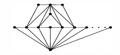
Figure 2: A nonhamiltonian locally linear graph of order $n$ with maximum vertex degree $n-5$.

Lemma 6.

The maximum degree of a nonhamiltonian locally linear graph with order $n$ is $n-5.$

Proof.

Let $G$ be a nonhamiltonian locally linear graph with $n$ vertices. To the contrary, suppose that $\Delta(G)\geq n-4$. It is obvious that $\Delta(G)\leq n-3$. Then we only need to consider the cases where $\Delta(G)=n-3$ and $\Delta(G)=n-4$. For convenience, let $u$ be a vertex in $G$ of degree $\Delta(G)$, and let $v_{1},v_{2},\ldots,v_{\Delta(G)}$ be an induced path of $G[N(u)]$.

Case 1. $\Delta(G)=n-3$.

Without loss of generality, we may assume that $V(G)-N[u]=\{x,y\}$. If $x\leftrightarrow y,$ by Observation 5 $(2)$, we have that $G$ is hamiltonian, a contradiction. Then we assume that $x\nleftrightarrow y.$ Clearly, $N(x)\cup N(y)\subseteq N(u)$. By Observation 5 $(1)$, there exist $i,j\in[n-4]$ and $i\leq j$ such that $\{v_{i},v_{i+1}\}\subseteq N(x)$ and $\{v_{j},v_{j+1}\}\subseteq N(y)$. Note that every edge of a locally linear graph belongs to at most two triangles. Thus, $i\neq j$. However, this implies that $u,v_{1},\ldots,v_{i},x,v_{i+1},\ldots,v_{j},y,v_{j+1},\ldots,v_{n-3},u$ is a Hamilton cycle, a contradiction.

Case 2. $\Delta(G)=n-4$.

Without loss of generality, we may assume that $\{x,y,z\}=V(G)-N[u]$.

Subcase 2.1. $G[\{x,y,z\}]$ is connected.

It is obvious that $G[\{x,y,z\}]$ is either a $P_{3}$ or a $K_{3}$.

If $G[\{x,y,z\}]$ is a $P_{3}$. For convenience, we use $x,y,z$ to denote $G[\{x,y,z\}]$. Since $x\nleftrightarrow z$ and $\{x,z\}\subseteq N(y)$, we deduce that $N(x)\cap N(y)\neq\emptyset$ and $N(z)\cap N(y)\neq\emptyset$. It is obvious that $d_{G[N(y)]}(x,z)\geq 2$. We claim that $d_{G[N(y)]}(x,z)\leq 3$. For otherwise, there exists $v_{i}\in N(y)\cap N(u)$ such that $\{v_{i-1},v_{i+1}\}\subseteq N(y)$. Note that $\{y,u,v_{i-1},v_{i+1}\}\subseteq N(v_{i})$ and $G[\{y,u,v_{i-1},v_{i+1}\}]$ is a cycle. This implies that $G[N(v_{i})]$ contains a cycle, a contradiction. If $d_{G[N(y)]}(x,z)=3$, then there exist $\{v_{i},v_{i+1}\}\subseteq N(y)\cap N(u)$ such that $x\leftrightarrow v_{i}$ and $z\leftrightarrow v_{i+1}$ by symmetry. However, it follows that

$$u,v_{1},\ldots,v_{i},x,y,z,v_{i+1},\ldots,v_{n-4},u$$

is a Hamilton cycle, a contradiction. If $d_{G[N(y)]}(x,z)=2$, then there exists $v_{i}\in N(x)\cap N(y)\cap N(z)\cap N(u)$. Since $G[N(v_{i})]$ is an induced path, $N(\{x,z\})\cap\{v_{i-1},v_{i+1}\}\neq\emptyset$. By symmetry, we may assume that $v_{i-1}\leftrightarrow x$. Then

$$u,v_{1},\ldots,v_{i-1},x,y,z,v_{i},\ldots,v_{n-4},u$$

is a Hamilton cycle, a contradiction.

If $G[\{x,y,z\}]$ is a $K_{3}$. Since $G$ is connected, $N(\{x,y,z\})\cap N(u)\neq\emptyset$. Without loss of generality, we may assume that $N(x)\cap N(u)\neq\emptyset$. Since $\{y,z\}\subseteq N(x)$, there exists $v_{i}\in N(x)\cap N(u)$ such that $v_{i}\in N(\{y,z\})$. By symmetry, we may assume that $v_{i}\leftrightarrow z$. Since $G[N(v_{i})]$ is an induced path, $(N(\{x,z\}))\cap\{v_{i-1},v_{i+1}\}\neq\emptyset$. By symmetry, we may assume that $v_{i-1}\leftrightarrow x$. Then

$$u,v_{1},\cdots,v_{i-1},x,y,z,v_{i},\cdots,v_{n-4},u$$

is a Hamilton cycle, a contradiction.

Subcase 2.2. $G[\{x,y,z\}]$ is not connected.

Clearly, either $G[\{x,y,z\}]=3K_{1}$ or $G[\{x,y,z\}]=K_{1}\cup K_{2}$.

If $G[\{x,y,z\}]=3K_{1}$, then there exist three vertices $v_{i},v_{j}$ and $v_{k}$ in $N(u)$ such that $\{v_{i},v_{i+1}\}\subseteq N(x)$, $\{v_{j},v_{j+1}\}\subseteq N(y)$ and $\{v_{k},v_{k+1}\}\subseteq N(z)$ by Observation 5 $(1)$. Note that every edge of a locally linear graph belongs to at most two triangles. Thus, $v_{i}$, $v_{j}$, and $v_{k}$ are distinct. Without loss of generality, we may assume that $i<j<k$. This implies that

$$u,v_{1},\ldots,v_{i},x,v_{i+1},\ldots,v_{j},y,v_{j+1},\ldots,v_{k},z,v_{k+1},\ldots,v_{n-4},u$$

is a Hamilton cycle, a contradiction.

If $G[\{x,y,z\}]=K_{1}\cup K_{2}$. Without loss of generality, we may assume that $x$ is an isolated vertex in $G[{x,y,z}]$. By Observation 5 $(1)$, there exists $v_{i}$ in $N(u)$ such that $\{v_{i},v_{i+1}\}\subseteq N(x),$ and by Observation 5$(2)$, there exists $v_{j}$ in $N(u)$ such that $v_{j}\leftrightarrow y$ and $v_{j+1}\leftrightarrow z$. Note that every edge of a locally linear graph belongs to at most two triangles and $G[\{v_{j},v_{j+1},y,z\}]$ is a diamond. Therefore, $i\neq j$. Without loss of generality, we may assume that $i<j$. This implies that

$$u,v_{1},\ldots,v_{i},x,v_{i+1},\ldots v_{j},y,z,v_{j+1},\ldots v_{n-4},u$$

is a Hamilton cycle, a contradiction.

Figure 2 illustrates a connected nonhamiltonian locally linear graph of order $n\geq 12$ with maximum vertex degree $n-5$. Hence, the bound is sharp.

This completes the proof of Lemma 6. ∎

Now we are ready to prove Theorem 1.

Proof of Theorem 1. To the contrary, let $G$ be a nonhamiltonian locally linear graph with order $n\leq 11$. By Lemma 4 and Lemma 6, we have $6\leq\Delta(G)\leq n-5$. Then we can deduce that $n\geq 11.$ Hence $n=11$ and $\Delta(G)=6.$ Furthermore, let $u$ be a vertex with degree 6, let $v_{1},v_{2},\ldots,v_{6}$ be an induced Hamilton path of $G[N(u)]$, and let $X=V(G)-N[u]$. For convenience, we may assume that $X=\{x,y,z,w\}$.

Case 1. $G[X]$ is hamiltonian.

Without loss of generality, suppose that $x,y,z,w,x$ is a Hamilton cycle in $G[X]$. Since $G$ is a locally linear graph, we can deduce that either $G[X]$ is a diamond or $G[X]=C_{4}$. Note that $G$ is $2$-connected, we have $|N(X)\cap N(u)|\geq 2$.

Subcase 1.1. $G[X]$ is a diamond.

By symmetry, suppose that $x\leftrightarrow z$. Note that every edge of a locally linear graph belongs to at most two triangles. Hence $N(z)\cap N(x)=\{y,w\}$. We claim that $N(x)\cap N(u)=\emptyset$. For otherwise, since $G[N(x)]$ is an induced path, there exists $v_{i}\in N(x)\cap N(u)$ such that $v_{i}\in N(\{y,w\})$. By symmetry, we assume that $v_{i}\leftrightarrow y$. Clearly, $v_{i}\notin N(\{w,z\})$. Since $G[N(v_{i})]$ is an induced path and $\{x,y,v_{i-1},v_{i+1}\}\subseteq N(v_{i})$, $N(\{x,y\})\cap\{v_{i-1},v_{i+1}\}\neq\emptyset$. Without loss of generality, we may assume that $v_{i+1}\in N(\{x,y\})$. This implies that either

$$u,v_{1},\ldots,v_{i},x,w,z,y,v_{i+1},\ldots,v_{6},u$$

is a Hamilton cycle, or

$$u,v_{1},\ldots,v_{i},y,z,w,x,v_{i+1},\ldots,v_{6},u$$

is a Hamilton cycle, a contradiction. Therefore, $N(x)\cap N(u)=\emptyset$. Similarly, we have $N(z)\cap N(u)=\emptyset$. This implies that $N(\{y,w\})\cap N(u)\neq\emptyset$. However, it follows that either $G[N(y)]$ or $G[N(w)]$ , one of them is disconnected, a contradiction.

Subcase 1.2. $G[X]=C_{4}$.

By symmetry, we may assume that $N(x)\cap N(u)\neq\emptyset$. On the one hand, since $G[N(x)]$ is an induced path, there exists $v_{i}\in N(x)$ such that $v_{i}\in N(\{y,w\})$. On the other hand, since $G[N(v_{i})]$ is an induced path, $N(\{x,y,w\})\cap\{v_{i-1},v_{i+1}\}$. We may assume up to symmetry that $v_{i+1}\leftrightarrow y$. This implies that

$$u,v_{1},\ldots,v_{i},x,w,z,y,v_{i+1},\ldots,v_{6},u$$

is a Hamilton cycle, a contradiction.

Case 2. $G[X]$ is nonhamiltonian but traceable.

Without loss of generality, suppose that $x,y,z,w$ is a Hamilton path in $G[X]$. Since $G[X]$ is nonhamiltonian, $\min\{d_{G[X]}(x),d_{G[X]}(w)\}=1$. By symmetry, we may assume that $d_{G[X]}(x)=1$. Since $\delta(G)\geq 2$ and $G[N(x)]$ is an induced path, there exists $v_{i}\in N(x)\cap N(y)\cap N(u)$. Note that $w\notin N(\{v_{i-1},v_{i+1}\})$.

Subcase 2.1. $w\nleftrightarrow y$.

Clearly, we have that $d_{G[X]}(w)=1$ and hence $N(w)\cap N(u)\neq\emptyset$. Since $G[N(w)]$ is an induced path, there is $v_{j}\in N(w)\cap N(z)\cap N(u)$. If $i=j$, then $i$ must belong to $\{1,6\}$, as $\Delta(G)=6.$ By symmetry, we may assume that $i=1$. Since $G[N(v_{1})]$ is an induced path and $N(v_{1})=\{x,y,z,w,u,v_{2}\}$, either $v_{2}\in N(x)$ or $v_{2}\in N(w)$. We may assume up to symmetry that $v_{2}\leftrightarrow w$. This implies that $u,v_{1},x,y,z,w,v_{2},\ldots,v_{6},u$ is a Hamilton cycle, a contradiction. Therefore, $i\neq j$. Without loss of generality, we may assume that $i<j$. If $i=1$, then $u,v_{6},\ldots,v_{j},w,z,y,x,v_{1},\ldots,v_{j-1},u$ is a Hamilton cycle, a contradiction. Therefore, $i\neq 1$. Similarly, $j\neq 6$. Note that $j\neq i+1$. By symmetry, we only need to consider the case where $i=2$ and $j\in\{4,5\}$.

Suppose $i=2$ and $j=4$. We claim that $\{x,w\}\cap N(v_{3})=\emptyset$. For otherwise, either

$$v_{3},v_{2},v_{1},u,v_{6},v_{5},v_{4},w,z,y,x,v_{3}$$

is a Hamilton cycle or

$$v_{3},v_{4},v_{5},v_{6},u,v_{1},v_{2},x,y,z,w,v_{3}$$

is a Hamilton cycle.

Since $x,y,z,w,v_{4},v_{5},v_{6},u,v_{3},v_{2},v_{1}$ and $w,z,y,x,v_{2},v_{3},v_{4},v_{5},v_{6},u,v_{1}$ are two Hamilton paths, $x\nleftrightarrow v_{1}$ and $w\nleftrightarrow v_{1}$. Similarly, $x,y,z,w,v_{4},v_{3},v_{2},v_{1},u,v_{5},v_{6}$ and $w,z,y,x,v_{2},v_{1},u,v_{3},v_{4},v_{5},v_{6}$ are two Hamilton paths. Thus, $x\nleftrightarrow v_{6}$ and $w\nleftrightarrow v_{6}$.

Suppose that $v_{2}\leftrightarrow w$. Then $N(v_{2})=\{v_{1},v_{3},u,x,y,w\}$. Since $N(w)\cap\{x,y,v_{1},v_{3},u\}=\emptyset$, $G[N(v_{2})]$ is disconnected , which contradicts the fact that $G[N(v_{2})]$ is an induced path. Thus, $v_{2}\nleftrightarrow w$.

Suppose that $v_{2}\leftrightarrow z$. It is obvious that $z\nleftrightarrow v_{3}$. Note that $N(v_{2})=\{v_{1},v_{3},u,x,y,z\}$ and $N(x)\cap\{v_{1},v_{3}\}=\emptyset$. Since $G[N(v_{2})]$ is an induced path, $z\leftrightarrow v_{1}$. Since $y,x,v_{2},v_{1},z,w,v_{4},v_{3},u,v_{5},v_{6}$ and $y,x,v_{2},v_{1},z,w,v_{4},v_{3},u,v_{6},v_{5}$ are two Hamilton paths, $N(y)\cap\{v_{5},v_{6}\}=\emptyset$. Since

$$y,x,v_{2},v_{1},z,w,v_{5},v_{6},u,v_{4},v_{4}$$

is a Hamilton path, $y\nleftrightarrow v_{4}$. Note that the set of $N(z)$ has three possibilities: $N(z)=\{y,w,v_{1},v_{2},v_{4}\}$, $N(z)=\{y,w,v_{1},v_{2},v_{4},v_{5}\}$ or $N(z)=\{y,w,v_{1},v_{2},v_{4},v_{6}\}$. It follows that $G[N(z)]$ is not an induced path, a contradiction. Therefore, $v_{2}\nleftrightarrow z$. This implies that $N(v_{2})=\{v_{1},u,v_{3},x,y\}$. Note that $x\nleftrightarrow v_{1}$ and $x\nleftrightarrow v_{3}$. Since $G[N(v_{2})]$ is an induced path, $y\in N(\{v_{1},v_{3}\})$.

Suppose that $y\leftrightarrow v_{4}$. Then $N(v_{4})=\{v_{3},u,v_{5},y,z,w\}$. Clearly, $y\nleftrightarrow v_{3}$. Hence, $y\leftrightarrow v_{1}$. Since

$$z,w,v_{4},v_{5},v_{6},u,v_{3},v_{2},x,y,v_{1}$$

is a Hamilton path, $z\nleftrightarrow v_{1}$. Note that $x\nleftrightarrow v_{5}$. If $y\leftrightarrow v_{5}$, then $N(y)=\{x,z,v_{1},v_{2},v_{4},v_{5}\}$. However, it follows that $G[N(y)]$ is not connected, a contradiction. Thus, $y\nleftrightarrow v_{4}$.

Suppose that $x\leftrightarrow v_{4}$. Then $N(v_{4})=\{v_{3},u,v_{5},x,z,w\}$. Note that $x\nleftrightarrow v_{3}$ and $x\nleftrightarrow v_{5}$. This implies that $G[N(v_{4})]$ is not connected, a contradiction. Thus, $x\nleftrightarrow v_{4}$. That is, $N(v_{4})=\{v_{3},u,v_{5},z,w\}$.

Suppose that $y\leftrightarrow v_{1}$. Since

$$z,w,v_{4},v_{5},v_{6},u,v_{1},y,x,v_{2},v_{3},$$

$$z,w,v_{4},v_{3},v_{2},x,y,v_{1},u,v_{6},v_{5}$$

and

$$w,z,v_{4},v_{3},v_{2},x,y,v_{1},u,v_{6},v_{5}$$

are three Hamilton paths, $z\notin N(\{v_{3},v_{5}\})$ and $w\nleftrightarrow v_{5}$. This implies that $G[N(v_{4})]$ is not connected, a contradiction. Hence, $y\nleftrightarrow v_{1}$ and so $y\leftrightarrow v_{3}$. Since

$$z,w,v_{4},v_{5},v_{6},u,v_{1},v_{2},x,y,v_{3},$$

$$z,w,v_{4},v_{3},y,x,v_{2},v_{1},u,v_{6},v_{5}$$

and

$$z,w,v_{4},v_{3},y,x,v_{2},v_{1},u,v_{6},v_{5}$$

are three Hamilton paths, $z\notin N(\{v_{3},v_{5}\})$ and $w\nleftrightarrow v_{5}$. This implies that $G[N(v_{4})]$ is not connected, a contradiction.

Therefore, $i=2$ and $j=5$. Clearly, $x\nleftrightarrow v_{6}$ and $w\nleftrightarrow v_{1}$. Since $x,y,z,w,v_{5},v_{6},u,v_{4},v_{3},v_{2},v_{1}$ is a Hamilton path, $x\nleftrightarrow v_{1}$. By symmetry, we have that $w\nleftrightarrow v_{6}$.

Suppose that $v_{2}\leftrightarrow z$.

If $z\leftrightarrow v_{3}$, then $N(v_{2})=\{x,y,z,v_{1},u,v_{3}\}$ and $v_{1},u,v_{3},z,y,x$ is a path. Since $G[N(v_{2})]$ is an induced path, $N(v_{3})\cap\{x,y\}=\emptyset$. Clearly, $z\nleftrightarrow v_{4}$. If $v_{1}\leftrightarrow z$, then $d_{G[N(z)]}(v_{2})\geq 3$. This implies that $G[N(z)]$ is not an induced path, a contradiction. Since $y,x,v_{2},v_{1},u,v_{4},v_{3},z,w,v_{5},v_{6}$ is a Hamilton path, $y\nleftrightarrow v_{6}$. If $y\leftrightarrow v_{5}$, then $N(v_{5})=\{y,z,w,v_{4},u,v_{6}\}$. Since

$$y,x,v_{2},v_{1},u,v_{6},v_{5},w,z,v_{3},v_{4}$$

and

$$w,v_{5},v_{6},u,v_{1},v_{2},x,y,z,v_{3},v_{4}$$

are two Hamilton paths, $y\nleftrightarrow v_{4}$ and $w\nleftrightarrow v_{4}$. This implies that $G[N(v_{5})]$ is not connected, a contradiction. Thus, $y\nleftrightarrow v_{5}$. Note that either $N(z)=\{y,v_{2},v_{3},v_{5},w\}$ or $N(z)=\{y,v_{2},v_{3},v_{5},w,v_{6}\}$. This implies that $G[N(z)]$ is not an induced path, a contradiction. Thus, $z\nleftrightarrow v_{3}$.

If $z\leftrightarrow v_{1}$, then $N(v_{2})=\{x,y,z,v_{1},u,v_{3}\}$ and $v_{3},u,v_{1},z,y,x$ is a path. Since $G[N(v_{2})]$ is an induced path, $v_{3},u,v_{1},z,y,x$ is an induced path. We claim that $y\nleftrightarrow v_{5}$. For otherwise, we assume that $y\leftrightarrow v_{5}$. Then, $N(v_{5})=\{y,z,w,v_{4},u,v_{6}\}$. If $y\leftrightarrow v_{4}$, then

$$y,x,v_{2},v_{1},z,w,v_{5},v_{6},u,v_{3},v_{4},y$$

is a Hamilton cycle, a contradiction. Hence, $y\nleftrightarrow v_{4}$. If $y\leftrightarrow v_{6}$, then

$$z,w,v_{5},v_{6},y,x,v_{2},v_{3},v_{4},u,v_{1},z$$

is a Hamilton cycle, a contradiction. Thus, $y\nleftrightarrow v_{6}$. Since $G[N(v_{5})]$ is an induced path and $w\nleftrightarrow v_{6}$, $w\leftrightarrow v_{4}$. However, it follows that $w,v_{5},v_{6},u,v_{1},z,y,x,v_{2},v_{3},v_{4},w$ is a Hamilton cycle, a contradiction. Therefore, $y\nleftrightarrow v_{5}$.

Note that the set of $N(z)$ has three possibilities: $N(z)=\{y,w,v_{1},v_{2},v_{4}\}$, $N(z)=\{y,w,v_{1},v_{2},v_{4},v_{5}\}$ or $N(z)=\{y,w,v_{1},v_{2},v_{4},v_{6}\}$. Since $y,x,v_{2},v_{1},z,w,v_{5},v_{6},u,v_{3},v_{4}$ and $y,x,v_{2},v_{1},z,w,v_{5},v_{4},v_{3},u,v_{6}$ are two Hamilton paths, $y\nleftrightarrow v_{4}$ and $y\nleftrightarrow v_{6}$. This implies that $G[N(z)]$ is not an induced path, a contradiction. Therefore, $z\nleftrightarrow v_{1}$.

Since $G[N(v_{2})]$ is an induced path and $N(v_{2})=\{v_{1},u,v_{3},x,y,z\}$, $x\leftrightarrow v_{3}$. If $z\leftrightarrow v_{6}$, then $z,w,v_{5},v_{4},v_{3},x,y,v_{2},v_{1},u,v_{6},z$ is a Hamilton cycle, a contradiction. So, $z\nleftrightarrow v_{6}$.

Since $z,w,v_{5},v_{6},u,v_{1},v_{2},y,x,v_{3},v_{4}$ is a Hamilton path, $z\nleftrightarrow v_{4}$. This implies that $N(z)=\{y,v_{2},w,v_{5}\}$. Note that $w\notin N(\{y,v_{2}\})$. Since $G[N(z)]$ is an induced path, $y\leftrightarrow v_{5}$. On the one hand, by the previous analysis on $z\nleftrightarrow v_{3}$, we have that $y\nleftrightarrow v_{4}$. On the other hand, by the previous analysis on $z\nleftrightarrow v_{i}$, we have that $y\nleftrightarrow v_{6}$. Since $N(v_{5})=\{y,z,w,v_{4},u,v_{6}\}$ and $G[N(v_{5})]$ is an induced path, $w\leftrightarrow v_{4}$. However, it follows that $x,v_{3},v_{4},w,z,v_{2},v_{1},u,v_{6},v_{5},y,x$ is a Hamilton cycle, a contradiction. Then, $v_{2}\nleftrightarrow z$.

Note that $w\nleftrightarrow v_{1}$ and $w\nleftrightarrow v_{3}$. Furthermore, if $w\leftrightarrow v_{2}$, then we have that $w\in N(\{v_{1},v_{3}\})$, a contradiction. Thus, $w\nleftrightarrow v_{2}$. Therefore, $N(v_{2})=\{v_{1},u,v_{3},x,y\}$. By symmetry, we have that $N(v_{5})=\{v_{4},u,v_{6},z,w\}$.

Since $z\leftrightarrow y$, $N(y)\cap N(z)\neq\emptyset$. Note that $v_{2}\nleftrightarrow z$. By symmetry, we have that $y\nleftrightarrow v_{5}$. Thus, we have that $\{v_{1},v_{3},v_{4},v_{6}\}\cap(N(y)\cap N(z))\neq\emptyset$. By symmetry, we only need to consider the cases that $v_{1}\in N(y)\cap N(z)$ and $v_{3}\in N(y)\cap N(z)$. If $v_{1}\in N(y)\cap N(z)$, then

$$w,v_{5},v_{6},u,v_{1},z,y,x,v_{2},v_{3},v_{4},$$

$$z,w,v_{5},v_{6},u,v_{1},y,z,v_{2},v_{3},v_{4}$$

and

$$z,w,v_{5},v_{4},v_{3},v_{2},x,y,v_{1},u,v_{6}$$

are three Hamilton paths. This implies that $N(\{z,w\})\cap\{v_{4},v_{6}\}=\emptyset$. However, it follows that $G[N(v_{5})]$ is not connected, a contradiction. If $v_{3}\in N(y)\cap N(z)$, then

$$w,v_{5},v_{6},u,v_{1},v_{2},x,y,z,v_{3},v_{4},$$

$$z,w,v_{5},v_{4},v_{3},y,x,v_{2},v_{1},u,v_{6}$$

and

$$z,w,v_{5},v_{6},u,v_{1},v_{2},x,y,v_{3},v_{4}$$

are three Hamilton paths. Thus, $N(\{z,w\})\cap\{v_{4},v_{6}\}=\emptyset$. Note that $N(v_{5})=\{v_{4},u,v_{6},z,w\}$. However, it follows that $G[N(v_{5})]$ is not an induced path, a contradiction.

Subcase 2.2. $w\leftrightarrow y$.

Since $G[N(y)]$ is an induced path and $\{x,z,w\}\subseteq N(y)$, there exists $v_{j}\in N(u)\cap N(y)$ such that$|N(v_{j})\cap\{z,w\}|=1$. By symmetry, we may assume that $v_{j}\leftrightarrow z$. If $i=j$, then $N(v_{i})=\{v_{i-1},v_{i+1},u,x,y,z\}$. Since $G[N(v_{i})]$ is an induced path, $\{v_{i-1},v_{i+1}\}\cap(N(x)\cup N(z))\neq\emptyset$. In all cases, we have that $G$ has a Hamilton cycle, a contradiction. Therefore, $i\neq j$ and $N(x)\cap N(\{z,w\})\cap N(y)=\emptyset$. Without loss of generality, we may assume that $i<j$. Clearly, $j\neq i+1$. Note that $\{w,v_{j}\}\cap N(\{x,v_{i}\})=\emptyset$. If $d(y)=5$, then $G[N(y)]$ is not connected, a contradiction. Thus, $d(y)=6$. This implies that there exists $v_{r}\in N(y)\cap N(u)$. Clearly, $v_{r}\notin N(x)\cap N(w)$. If $v_{r}\leftrightarrow x$, then $v_{r}\leftrightarrow v_{j}$ since $G[N(y)]$ is an induced path. Thus, either $v_{r}=v_{j-1}$ or $v_{r}=v_{j+1}$. In any cases, we have that $G$ has a Hamilton cycle, a contradiction. Thus, $v_{r}\nleftrightarrow x$. If $v_{r}\leftrightarrow w$, then $v_{r}\leftrightarrow v_{i}$ since $G[N(y)]$ is an induced path. Hence, either $v_{r}=v_{i-1}$ or $v_{r}=v_{i+1}$. In any cases, we have that $G$ has a Hamilton cycle, a contradiction. Therefore, $v_{r}\nleftrightarrow w$. since $G[N(y)]$ is an induced path and $N(\{x,v_{i}\})\cap N(\{w,z,v_{j}\})=\emptyset$, $v_{r}\in N(v_{i})\cap N(v_{j})$. That is, $r=i+1$ and $j=i+2$. Note that $\{y,v_{i},v_{i+1},u\}\subseteq N(v_{i+1})$ and $y,v_{i},u,v_{i+1},y$ is a cycle. This implies that $G[N(v_{i+1})]$ contains a cycle and hence not an induced path, a contradiction.

Case 3. $G[X]=K_{1,3}$.

Without loss of generality, we may assume that $\{y,z,w\}\subseteq N(x)$. Since $\{y,z,w\}$ forms an independent set and $G[N(x)]$ is an induced path, we have $d_{G}(x)\geq 5$.

Subcase 3.1. $d_{G}(x)=5$.

Note that $d_{G}(x)=5$, there must exist ${v_{i},v_{j}}\subseteq N(x)\cap N(u)$. We may assume by the symmetry that $G[N(x)]=y,v_{i},z,v_{j},w$. We claim that $\{v_{i},v_{j}\}\cap\{v_{1},v_{6}\}=\emptyset$. For otherwise, suppose that $v_{i}=v_{1}$ by symmetry. Note that $\{y,z,w,u\}$ is an independent set and $\Delta(G)=6$. By Observation 5 $(3)$, we have that $w\notin N(v_{1})$. Thus, $N(v_{1})=\{x,y,z,v_{2},u\}$. Since $G[N(v_{1})]$ is an induced path, $v_{2}\in N(\{y,z\})$. If $v_{2}\leftrightarrow z$, then $x,w,v_{j},\ldots,v_{6},u,v_{j-1},\cdots,v_{2},z,v_{1},y,x$ is a Hamilton cycle, a contradiction. If $v_{2}\leftrightarrow y$, then $x,w,v_{j},\ldots,v_{6},u,v_{j-1},\ldots,v_{2},y,v_{1},z,x$ is a Hamilton cycle, a contradiction. Therefore, $\{v_{i},v_{j}\}\cap\{v_{1},v_{6}\}=\emptyset$. Without loss of generality, we may assume that $i<j$. Note that $G[N(x)]=y,v_{i},z,v_{j},w$. Thus, $v_{i}\nleftrightarrow v_{j}$, implying that $j>i+1$. By symmetry, we need only consider the cases where $i=2$ and $j=4$, or $i=2$ and $j=5$.

Suppose that $i=2$ and $j=4$. Clearly, $z\nleftrightarrow v_{3}$. Note that $N(v_{4})=\{v_{3},u,v_{5},x,z,w\}$. Since $G[N(v_{4})]$ is an induced path, either $w\in N(\{v_{3},v_{5}\})$ or $z\in N(v_{5})$. If $w\leftrightarrow v_{3}$, then

$$y,x,z,v_{2},v_{3},w,v_{4},v_{5},v_{6},u,v_{1},$$

$$y,x,z,v_{2},v_{1},u,v_{6},v_{5},v_{4},w,v_{3}$$

and

$$z,x,y,v_{2},v_{3},w,v_{4},v_{5},v_{6},u,v_{1}$$

are three Hamilton paths. Since $G$ is nonhamiltonian, we have $N(\{v_{1},v_{3}\})\cap\{y,z\}=\emptyset$. This implies that $G[N(v_{2})]$ is not connected, a contradiction. If $w\leftrightarrow v_{5}$, then

$$y,x,z,v_{4},w,v_{5},v_{6},u,v_{3},v_{2},v_{1},$$

$$y,v_{2},v_{1},u,v_{6},v_{5},w,x,z,v_{4},v_{3}$$

and

$$z,x,y,v_{2},v_{3},v_{4},w,v_{5},v_{6},u,v_{1}$$

are three Hamilton paths. Since $G$ is nonhamiltonian, $N(\{v_{1},v_{3}\})\cap\{y,z\}=\emptyset$. This implies that $G[N(v_{2})]$ is not connected, a contradiction. If $z\leftrightarrow v_{5}$, then

$$y,x,w,v_{4},v_{3},v_{2},z,v_{5},v_{6},u,v_{1},$$

$$y,x,w,v_{4},z,v_{5},v_{6},u,v_{1},v_{2},v_{3}$$

and

$$z,v_{5},v_{6},u,v_{3},v_{4},w,x,y,v_{2},v_{1}$$

are three Hamilton paths. By the same reason, we have $N(\{v_{1},v_{3}\})\cap\{y,z\}=\emptyset$. Then $G[N(v_{2})]$ is not connected, a contradiction. Now we have $w\notin N(\{v_{3},v_{5}\})$ and $z\notin N(v_{5})$. Note that $z\notin N(v_{3}).$ Hence, we have $N(\{v_{3},v_{5}\})\cap\{w,z\}=\emptyset$, which implies that $G[N(v_{5})]$ is not connected, leading to a contradiction.

Suppose that $i=2$ and $j=5$. Note that $N(v_{5})=\{v_{4},u,v_{6},x,z,w\}$. Since $G[N(v_{5})]$ is an induced path, $\{w,z\}\subseteq N(\{v_{4},v_{6}\})$. If $w\leftrightarrow v_{4}$, then

$$y,x,z,v_{2},v_{3},v_{4},w,v_{5},v_{6},u,v_{1},$$

$$y,x,z,v_{2},v_{1},u,v_{6},v_{5},w,v_{4},v_{3},$$

$$z,x,y,v_{2},v_{3},v_{4},w,v_{5},v_{6},y,v_{1}$$

and

$$z,x,y,v_{2},v_{1},u,v_{6},v_{5},w,v_{4},v_{3}$$

are four Hamilton paths. Since $G$ is nonhamiltonian, $N(\{v_{1},v_{3}\})\cap\{y,z\}=\emptyset$. This implies that $G[N(v_{2})]$ is not connected, a contradiction. If $w\leftrightarrow v_{6}$, then

$$y,x,w,v_{6},v_{5},z,v_{2},v_{3},v_{4},u,v_{1},$$

$$y,x,w,v_{6},v_{5},z,v_{2},v_{1},u,v_{4},v_{3},$$

$$z,x,y,v_{2},v_{1},u,v_{6},w,v_{5},v_{4},v_{3}$$

and

$$z,x,y,v_{2},v_{3},v_{4},v_{5},w,v_{6},u,v_{1}$$

are four Hamilton paths. Since $G$ is nonhamiltonian, $N(\{v_{1},v_{3}\})\cap\{y,z\}=\emptyset$. This implies that $G[N(v_{2})]$ is not connected, a contradiction. If $z\leftrightarrow v_{4}$, then

$$z,v_{4},v_{3},u,v_{6},v_{5},w,x,y,v_{2},v_{1},$$

$$y,x,w,v_{5},v_{6},u,v_{3},v_{4},z,v_{2},v_{1}$$

and

$$y,x,w,v_{5},v_{6},u,v_{1},v_{2},z,v_{4},v_{3}$$

are three Hamilton paths. Clearly, $z\nleftrightarrow v_{3}$. Since $G$ is nonhamiltonian, $N(\{v_{1},v_{3}\})\cap\{y,z\}=\emptyset$. This implies that $G[N(v_{2})]$ is not connected, a contradiction. If $z\leftrightarrow v_{6}$, then

$$y,x,w,v_{5},v_{6},z,v_{2},v_{3},v_{4},u,v_{1},$$

$$y,x,w,v_{5},v_{6},z,v_{2},v_{1},u,v_{4},v_{3}$$

and

$$z,v_{6},v_{5},w,x,y,v_{2},v_{1},u,v_{4},v_{3}$$

are four Hamilton paths. Since $G$ is nonhamiltonian, $N(\{v_{1},v_{3}\})\cap\{y,z\}=\emptyset$. This implies that $G[N(v_{2})]$ is not connected, a contradiction. Therefore, $\{w,z\}\cap N(\{v_{4},v_{6}\})=\emptyset$, which implies that $G[N(v_{5})]$ is not connected, leading to a contradiction.

Subcase 3.2. $d_{G}(x)=6$.

By symmetry, either $G[N(x)]=y,v_{i},z,v_{j},w,v_{r}$ or $G[N(x)]=y,v_{i},z,v_{j-1},v_{j},w$.

Suppose that $G[N(x)]=y,v_{i},z,v_{j},w,v_{r}$. We claim that $\{v_{i},v_{j},v_{r}\}\cap\{v_{1},v_{6}\}=\emptyset$. For otherwise, assume that $v_{i}=v_{1}$. By Observation 5 $(3)$, we have that $N(v_{1})=\{x,y,z,v_{2},u\}$. Since $G[N(x)]$ is an induced path, $v_{2}\notin\{v_{j},v_{r}\}$. However,

$$z,v_{1},y,x,w,v_{r},\ldots,v_{6},u,v_{r-1},\ldots,v_{2}$$

and

$$y,v_{1},z,x,w,v_{r},\ldots,v_{6},u,v_{r-1},\ldots,v_{2}$$

are two Hamilton paths. Since $G$ is nonhamiltonian, $v_{2}\notin N(\{y,z\})$. This implies that $G[N(v_{1})]$ is not connected, a contradiction. Therefore, $v_{i}\neq v_{1}$. By symmetry, we have $v_{i}\neq v_{6}$. Similarly, we have $v_{j}\notin\{v_{1},v_{6}\}$.

If $v_{1}=v_{r}$, then $N(v_{1})=\{x,w,v_{2},u\}$. Since $G[N(x)]$ is an induced path, $v_{2}\notin\{v_{i},v_{j}\}$. It follows that $v_{2}\nleftrightarrow x$. Since $G[N(v_{1})]$ is an induced path, $w\leftrightarrow v_{2}$. It is obvious that $\{v_{i},v_{j}\}\subseteq\{v_{3},v_{4},v_{5}\}$. Since $v_{i}\nleftrightarrow v_{j}$, $\{v_{i},v_{j}\}=\{v_{3},v_{5}\}$. If $v_{i}=v_{5}$ and $v_{j}=v_{3}$, then $N(v_{5})=\{v_{4},u,v_{6},x,y,z\}$. Note that

$$y,v_{5},v_{6},u,v_{2},v_{1},w,x,z,v_{3},v_{4},$$

$$y,v_{5},v_{4},v_{3},z,x,w,v_{2},v_{1},u,v_{6}$$

and

$$z,v_{3},v_{4},v_{5},y,x,w,v_{2},v_{1},u,v_{6}$$

are three Hamilton paths. Clearly, $z\nleftrightarrow v_{4}$. This implies that $N(v_{5})$ is not connected, a contradiction. If $v_{i}=v_{3}$ and $v_{j}=v_{5}$, then $N(v_{5})=\{v_{4},u,v_{6},x,z,w\}$. Note that

$$z,v_{5},v_{4},v_{3},y,x,w,v_{2},v_{1},u,v_{6},$$

$$w,v_{1},v_{2},u,v_{4},v_{3},y,x,z,v_{5},v_{6}$$

and

$$w,v_{1},v_{2},u,v_{6},v_{5},z,x,y,v_{3},v_{4}$$

are three Hamilton paths. Clearly, $z\nleftrightarrow v_{4}$. Since $G$ is nonhamiltonian, $\{v_{4},v_{6}\}\cap N(\{z,w\})=\emptyset$. This implies that $N(v_{5})$ is not connected. Therefore, $\{v_{i},v_{j},v_{r}\}\cap\{v_{1},v_{6}\}=\emptyset$. Since $G[\{v_{2},v_{3},v_{4},v_{5}\}]$ is an induced path, $\alpha(G[\{v_{2},v_{3},v_{4},v_{5}\}])=2$. Note that $\{v_{i},v_{j},v_{r}\}$ is an independent set and $\{v_{i},v_{j},v_{r}\}\subseteq\{v_{2},v_{3},v_{4},v_{5}\}$. This implies that $\alpha(G[\{v_{2},v_{3},v_{4},v_{5}\}])\geq 3$, a contradiction.

Therefore, $G[N(x)]=y,v_{i},z,v_{j-1},v_{j},w$. Without loss of generality, we may assume that $i<j$. If $v_{i}=v_{1}$, then $v_{1},y,x,w,v_{j},\ldots,v_{6},u,v_{2},\ldots,v_{j-1},z,v_{1}$ is a Hamilton cycle, a contradiction. If $v_{j}=v_{6}$, then

$$y,v_{i},z,x,w,v_{6},v_{5},\ldots,v_{i+1},u,v_{1},\ldots,v_{i-1},$$

$$y,v_{i},v_{i-1},\ldots,v_{1},u,v_{6},w,x,z,v_{5},\ldots,v_{i+1},$$

$$z,v_{5},v_{6},w,x,y,v_{i},v_{i-1},\ldots,v_{1},u,v_{j-2},\ldots,v_{i+1}$$

and

$$z,v_{5},v_{6},w,x,y,v_{i},v_{i+1},\ldots,v_{j-2},u,v_{1},\ldots,v_{i-1}$$

are four Hamilton paths. Since $G$ is nonhamiltonian, $\{v_{i-1},v_{i+1}\}\cap N(\{y,z\})=\emptyset$. Note that $N(v_{i})=\{v_{i-1},v_{i+1},u,x,y,z\}$. Thus, $G[N(v_{i})]$ is not connected. Therefore, $i=2$ and $j=5$. Clearly, $z\nleftrightarrow v_{3}$. Since $y,v_{2},v_{1},u,v_{6},v_{5},w,x,z,v_{4},v_{3}$ and $y,v_{2},v_{3},v_{4},z,x,w,v_{5},v_{6},u,v_{1}$ are two Hamilton paths, $y\notin N(\{v_{1},v_{3}\}).$ Note that $N(v_{2})=\{v_{1},u,v_{3},x,y,z\}$ and $G[N(v_{2})]$ is an induced path. This implies that $z\leftrightarrow v_{1}$. However, $z,v_{1},u,v_{6},v_{5},w,x,y,v_{2},v_{3},v_{4},z$ is a Hamilton cycle, a contradiction.

Case 4. $G[X]=K_{1}\cup K_{3}$.

Without loss of generality, we assume that $x$ is an isolated vertex in $G[X]$. Clearly $N(\{y,z,w\})\cap N(u)\neq\emptyset$. By symmetry, assume that $N(y)\cap N(u)\neq\emptyset$. On the one hand, since $\{z,w\}\subseteq N(y)$ and $N(y)\cap N(u)\neq\emptyset$, there exists $v_{i}\in N(y)\cap N(u)$ such $v_{i}\in N(\{z,w\})$. By symmetry, we may assume that $v_{i}\in N(z)$. On the other hand, since $\{y,z,v_{i-1},v_{i+1}\}\subseteq N(v_{i})$ and $G[N(v_{i})]$ is an induced path, $\{v_{i-1},v_{i+1}\}\cap N(\{y,z\})\neq\emptyset$. Without loss of generality, we may assume that $v_{i+1}\leftrightarrow z$. By Observation 5 $(1)$, there exists $v_{j}\in N(u)$ such that $\{v_{j},v_{j+1}\}\subseteq N(x)$. Note that every edge of a locally linear graph belongs to at most two triangles. Thus, $i\neq j$. By symmetry, we may assume that $i<j$. However, it follows that $u,v_{1},\ldots,v_{i},y,w,z,v_{i+1},\ldots,v_{j},x,v_{j+1},\ldots,v_{6},u$ is a Hamilton cycle, a contradiction.

Case 5. $G[X]=K_{1}\cup P_{3}$.

Without loss of generality, we assume that $w$ is an isolated vertex in $G[X]$ and $G[\{x,y,z\}]=x,y,z$. By Observation 5 $(1)$, there exists $v_{j}\in N(u)$ such that $\{v_{j},v_{j+1}\}\subseteq N(w)$. Since $x\nleftrightarrow z$ and $\{x,z\}\subseteq N(y)$, $N(x)\cap N(y)\neq\emptyset$ and $N(z)\cap N(y)\neq\emptyset$. It is obvious that $d_{G[N(y)]}(x,z)\geq 2$. We claim that $d_{G[N(y)]}(x,z)\leq 3$. For otherwise, there exists $v_{i}\in N(y)\cap N(u)$ such that $\{v_{i-1},v_{i+1}\}\subseteq N(y)$. Note that $\{y,u,v_{i-1},v_{i+1}\}\subseteq N(v_{i})$ and $G[\{y,u,v_{i-1},v_{i+1}\}]$ is a cycle. This implies that $G[N(v_{i})]$ contains a cycle, a contradiction. If $d_{G[N(y)]}(x,z)=3$, then there exist $\{v_{i},v_{i+1}\}\subseteq N(y)\cap N(u)$ such that $x\leftrightarrow v_{i}$ and $z\leftrightarrow v_{i+1}$ by symmetry. Note that every edge of a locally linear graph belongs to at most two triangles. Thus, $i\neq j$. By symmetry, we may assume that $i<j$. However, it follows that $u,v_{1},\ldots,v_{i},x,y,z,v_{i+1},\ldots,v_{j},w,v_{j+1},\ldots,v_{6},u$ is a Hamilton cycle, a contradiction. Therefore, $d_{G[N(y)]}(x,z)=2$. That is, there exists $v_{i}\in N(y)\cap N(u)$ such that $v_{i}\in N(x)\cap N(z)$. If $v_{i}=v_{1}$, then $N(v_{1})=\{v_{2},u,z,y,z\}$. Since $G[N(v_{1})]$ is an induced path, $v_{2}\in N(\{x,z\})$. We assume up to symmetry that $z\leftrightarrow v_{2}$. Clearly, $j\neq 1$. However, it follows that $u,v_{1},x,y,z,v_{2},\ldots,v_{j},w,v_{j+1},\ldots,v_{6},u$ is a Hamilton cycle, a contradiction. Similarly, $v_{i}\neq v_{6}$. Hence, $N(v_{i})=\{v_{i-1},v_{i+1},u,x,y,z\}$. Since $G[N(v_{i})]$ is an induced path, $\{v_{i-1},v_{i+1}\}\cap N(\{x,z\})\neq\emptyset.$ By symmetry, we may assume that $v_{i+1}\leftrightarrow z$ and $i<j$. This implies that

$$u,v_{1},\ldots,v_{i},x,y,z,v_{i+1},\ldots,v_{j},w,v_{j+1},\ldots,v_{6},u$$

is a Hamilton cycle, a contradiction.

Case 6. $G[X]=2K_{2}$.

Without loss of generality, we may assume that $\{xy,zw\}\subseteq E(G)$. By Observation 5 $(2)$, there exist $v_{i}$ and $v_{j}$ such that $G[\{x,y,v_{i},v_{i+1}\}]$ and $G[\{z,w,v_{j},v_{j+1}\}]$ are two diamonds. Note that every edge of a locally linear graph belongs to at most two triangles. Thus, $i\neq j$. By symmetry, we may assume that $\{xv_{i},yv_{i+1},zv_{j},wv_{j+1}\}\subseteq E(G)$ and $i<j$. This implies that

$$u,v_{1},\ldots,v_{i},x,y,v_{i+1},\ldots,v_{j},z,w,v_{j+1},\ldots,v_{6},u$$

is a Hamilton cycle, a contradiction.

Case 7. $G[X]=4K_{1}$.

By Observation 5 $(1)$, there exist four vertices $\{v_{i},v_{j},v_{k},v_{r}\}\subseteq N(u)$ such that $\{v_{i},v_{i+1}\}\subseteq N(x)$, $\{v_{j},v_{j+1}\}\subseteq N(y)$, $\{v_{k},v_{k+1}\}\subseteq N(z)$ and$\{v_{r},v_{r+1}\}\subseteq N(w)$. Note that every edge of a locally linear graph belongs to at most two triangles. Thus, $v_{i},v_{j},v_{k},v_{r}$ are distinct four vertices. Without loss of generality, we may assume that $i<j<k<r$. However, it follows that

$$u,v_{1},\ldots,v_{i},x,v_{i+1},\ldots,v_{j},y,v_{j+1},\ldots,v_{k},z,v_{k+1},\ldots,v_{r},w,v_{r+1},\ldots,v_{6},u$$

is a Hamilton cycle, a contradiction.

Figure 3 illustrates a connected nonhamiltonian locally linear graph of order $12$. Hence, the bound is sharp. This completes the proof of Theorem 1. $\Box$

Figure 3: A connected nonhamiltonian locally linear graph of order $12$.

3 The minimum size of nonhamiltonian locally traceable graphs

In this section, we will present the proof of Theorem 2. van Aardt and de Wet [7] provided the following procedure, called edge identification of two locally traceable graphs. For edge identification, a suitable edge in a graph $G$ is defined as an edge $uv$ such that there is a Hamilton path in $G[N(u)]$ that ends at $v$ and a Hamilton path in $G[N(v)]$that ends at $u$.

Construction 7 ([7]).

Let $G_{1}$ and $G_{2}$ be two locally traceable graphs such that $E(G_{i})$ contains a suitable edge $u_{i}v_{i},i=1,2$. Now create a graph $G$ of order $|V(G_{1})|+|V(G_{2})|-2$ by identifying the vertices $u_{1}$ and $u_{2}$ and the vertices $v_{1}$ and $v_{2}$ and call the resulting vertices $u$ and $v$, while retaining all the edges present in the original two graphs. We say that $G$ is obtained from $G_{1}$ and $G_{2}$ by identifying suitable edges.

Observation 8 ([7]).

Let $v$ be a vertex of degree two in a locally traceable graph. Then any edge incident with $v$ is suitable for use in edge identification.

Lemma 9 ([6]).

Let $G_{1}$ and $G_{2}$ be two locally traceable graphs, each with order at least $3$, and let $G$ be a graph obtained from $G_{1}$ and $G_{2}$ by identifying suitable edges. Then the following hold.

• $G$ is locally traceable;

• If $G_{1}$ and $G_{2}$ are planar, then $G$ is planar;

• If $G$ is hamiltonian, so are both $G_{1}$ and $G_{2}$.

An embedding of a graph $G$ on an orientable surface $\Sigma$ is minimal if $G$ cannot be embedded on any orientable surface $\Sigma^{\prime}$ where $g(\Sigma^{\prime})<g(\Sigma)$. A graph $G$ is said to have orientable genus $g$ if $G$ is minimally embedded on a surface with orientable genus $g$. An embedding of a graph is said to be $2$-cell if every face of the embedding is homomorphic to an open unit disk. The Euler characteristic of a graph $G$ is defined as follows.

$$\Phi(G)=2-2g.$$ (1)

If $G$ is a connected graph with a $2$-cell embedding on a closed surface, then Euler formula indicates that $n-m+f=\Phi(G)$.

The following results are needed in our proofs.

Theorem 10 ([19]).

If a connected graph $G$ is minimally embedded on an orientable surface, then the embedding is $2$-cell.

For a graph $G$, we denote $t(G)$ to be the number of triangles in $G$. For an edge $e$, let $t_{G}(e)$ be the number of triangles containing the edge $e$ in $G$. When $G$ is clear, we often drop the subscript. Let $g$ be a orientable genus of graph $G$ and embedding $G$ on some orientable surface $\Sigma$ with orientable genus $g$. Let $F(G)$ denote the set of faces in which graph $G$ lies within the orientable surface $\Sigma$, and let $B(G)$ denote the set of faces in which graph $G$ lies within the orientable surface $\Sigma$ that are not triangles. Clearly, $B(G)\subseteq F(G)$ and $t(G)+|B(G)|=|F(G)|$. For a face $f\in F(G)$. The degree of $f$ , denoted by $d(f)$, is the number of edges incident with it, where each cut-edge is counted twice.

Now we are ready to prove Theorem 2.

Proof of Theorem 2. Let $g$ be an integer, and let $g$ be a orientable genus of graph $G$ and embedding $G$ on some orientable surface $\Sigma$ with orientable genus $g$. By Theorem 10, the embedding is $2$-cell. Note that every edge of a locally linear graph belongs to at most two triangles. Furthermore, we refer to the edges in $G$ that belong to a triangle as $1$-edges, and the rest as $2$-edges. Clearly, each vertex in $G$ is incident to exactly two $1$-edges. Given that each vertex in $G$ is incident to exactly two $1$-edges, it follows that every vertex in $G$ and its corresponding two $1$-edges must belong to a face within $B(G)$. This implies that each face in $B(G)$ is an induced cycle. Note that each edge is only incident with two faces. Since $\sum_{f\in F(G)}d(f)=2m$, $3t(G)+n=2m$. That is, $3(|F(G)|)-|B(G)|=2m-n$. Then, $m-2n=3(|B(G)|-\Phi(G))$. Suppose that $m<2n$. That is, $|B(G)|<\Phi(G)$. Since $\Phi(G)=2-2g$ and $|B(G)|\geq 1$, $|B(G)|=1$. This implies that $G$ is hamiltonian, a contradiction.

By Theorem 1, we have that $n\geq 12$. When $n=12$, Figure 3 illustrates a connected nonhamiltonian locally linear graph of order $12$ with $24$ edges. Let $G_{12}$ be the graph depicted in Figure 3. For each $i\geq 13$, let $G_{i}$ be the graph obtained by combining $G_{i-1}$ with a $K_{3}$ by means of edge identification, starting with the edge $uv$, and after that each time using the edge between the vertices of degree two and three of the last added triangle, as shown in Figure 4. It follows from repeated application of Lemma 9 $(c)$ that for $i\geq 13$, the $G_{i}$ is a nonhamiltonian graph with $i$ vertices and $2i$ edges. We claim that $G_{i}$ is locally linear for all $i\geq 13$. For otherwise, there exists some $k$ such that $G_{k}$ is not locally linear. Among these, choose the $k$ is as small as possible. Clearly, $k\geq 13$. Note that $G_{k}$ is obtained from $G_{k-1}$ and $K_{3}$ by identifying the edge between the vertices of degree two and three of the last added triangle. That is, there exists a vertex $x$ of degree two such that $G_{k}-x=G_{k-1}$. Without loss of generality, we assume that $N_{G_{k}}(x)=\{y,z\}$. Note that $y\leftrightarrow z$ and $G_{k-1}$ is locally linear. Then, either $G_{k}[N_{G_{k}}(y)]$ is not an induced path or $G_{k}[N_{G_{k}}(z)]$ is not an induced path. Note that the edge $yz$ is incident to a vertex of degree two in $G_{k-1}$. Without loss of generality, we assume that $d_{G_{k-1}}(y)=2$ and $N_{G_{k-1}}(y)=\{z,w\}$. It is obvious that $G_{k}[N_{G_{k}}(y)]=w-z-x$ is an induced path. This implies that $G_{k}[N_{G_{k}}(z)]$ is not an induced path. However, Since $G_{k-1}$ is locally linear and $d_{G_{k-1}[N(z)]}(y)=1$, $G_{k-1}[N(z)]$ is an induced path with endpoints $y$. It follows that $G_{k}[N_{G_{k}}(z)]=G_{k-1}[N_{G_{k-1}}(z)]-x$ is an induced path, a contradiction. Therefore, $G_{i}$ is locally linear for all $i\geq 13$, completing the proof of this theorem. $\Box$

Figure 4: Constructing nonhamiltonian locally linear graphs with $m=2n$.

Proof of Theorem 3. Let $g$ be an integer, and let $g$ be a orientable genus of graph $G$ and embedding $G$ on some orientable surface $\Sigma$ with orientable genus $g$. By Theorem 10, the embedding is $2$-cell. Note that every edge of a locally linear graph belongs to at most two triangles. Furthermore, we refer to the edges in $G$ that belong to a triangle as $1$-edges, and the rest as $2$-edges. Clearly, each vertex in $G$ is incident to exactly two $1$-edges. Given that each vertex in $G$ is incident to exactly two $1$-edges, it follows that every vertex in $G$ and its corresponding two $1$-edges must belong to a face within $B(G)$. This implies that each face in $B(G)$ is an induced cycle. Note that each edge is only incident with two faces. Since $\sum_{f\in F(G)}d(f)=2m$, $3t(G)+n=2m$. That is, $3(|F(G)|-|B(G)|)=2m-n$. Then, $m-2n=3(|B(G)|-\Phi(G))$. By Theorem 2, we have $m\geq 2n$. Since $3|(m-2n)$, either $m=2n$ or $m\geq 2n+3$. If $m=2n$, then $|B(G)|=\Phi(G)$. Note that $\Phi(G)=2-2g$ and $|B(G)|\geq 1$. Then, $|B(G)|=2$. Without loss of generality, we assume that $B(G)=\{f_{1},f_{2}\}$. Note that $f_{1}$ and $f_{2}$ are two induced cycles and $V(f_{1})\cup V(f_{2})=V(G)$. Since $G$ is connected, there exist $u\in V(f_{1})$ and $v\in V(f_{2})$ such that $u\leftrightarrow v$. This implies that $G$ is traceable, a contradiction. Thus, $m\geq 2n+3$, completing the proof of this theorem. $\Box$

Acknowledgement. The authors are grateful to Professor Xingzhi Zhan for suggesting the problems in this paper. The authors also thank Doctor Yanan Hu for careful reading an early draft of this paper and for helpful comments. This research was supported by the NSFC grant 12271170 and Science and Technology Commission of Shanghai Municipality (STCSM) grant 22DZ2229014.

References

[1] S.A. van Aardt, M. Frick, O. Oellermann, J. P. de Wet, Global cycle properties in locally connected, locally traceable and locally hamiltonian graphs, Discrete Appl. Math. 205 (2016) 171-179.
[2] A.S. Asratian, N. Oksimets, Graphs with Hamiltonian Balls, Australasian Journal of Combinatorics 17 (1998) 185-198.
[3] J. A. Bondy, U. S. R. Murty, Graph theory. Graduate texts in mathematics, vol. 244. Springer, New York, 2008, pp. xii+651.
[4] B.L. Chilton, R. Gould, A.D. Polimeni, A note on graphs whose neighborhoods are -cycles, Geom. Dedicata 3 (1974) 289-294.
[5] J. Davies, C. Thomassen, Locally Hamiltonian graphs and minimal size of maximal graphs on a surface, Electron. J. Combin. 27 (2020) Paper No. 2.25.
[6] J.P. de Wet, M. Frick, S.A. van Aardt, Hamiltonicity of locally hamiltonian and locally traceable graphs, Discrete Appl. Math. 236 (2018) 137-152.
[7] J.P. de Wet, S.A. van Aardt, Traceability of locally traceable and locally hamiltonian graphs, Discrete Math. Theor. Comput. Sci. 17 (2016) 245-262.
[8] A.L. Gavrilyuk, A.A. Makhnev, Terwilliger graphs in which the neighborhood of some vertex is isomorphic to a petersen graph, Dokl. Math. 78 (2008) 550-553.
[9] A.L. Gavrilyuk, A.A. Makhnev, D.V. Paduchikh, On graphs in which the neighborhood of each vertex is isomorphic to the gewirtz graph, Dokl. Math. 80 (2009) 684-688.
[10] M.L. Kardanova, A.A. Makhnevb, D.V. Paduchikh, On graphs in which the neighborhood of each vertex is isomorphic to the higman-sims graph, Dokl. Math. 84 (2011) 471-474.
[12] R.C. Laskar, H.M. Mulder, B. Novick, Maximal outerplnar graphs as chordal graphs, path-neighborhood graphs, and triangle graphs, Australas. J. Combin. 52 (2012) 185-195.
[13] C.M. Pareek, On the maximum degree of locally Hamiltonian non-Hamiltonian graphs, Utilitas Math. 23 (1983) 103-120.
[14] C. M. Pareek, Z. Skupień, On the smallest non-hamiltonian locally hamiltonian graph, J. Univ. Kuwait (Sci.) 10 (1983) 9-17.
[15] T.D. Parsons, T. Pisanski, Graphs which are locally paths, in: Combinatorics and Graph Theory, Vol. 25, Banach Center Publ., PWN, Warsaw,1989, pp. 127-135.
[17] Z. Skupień, Locally Hamiltonian and planar graphs, Fund. Math, 58 (1966) 193–200.
[18] L. Tang, E Vumar, A Note on Cycles in Locally Hamiltonian and Locally Hamilton-Connected Graphs, Discussiones Mathematicae Graph Theory 40 (2020) 77-84.
[19] J.W.T. Youngs, Minimal imbedding and the genus of a graph, J. Math. Mech. 12 (1963) 303-315.
[20] H. Yu, B. Wu, Graphs in which is a cycle for each vertex , Discrete Math. 344 (2021) 112519.