Conformal structure of singularities in some varying fundamental constants bimetric cosmologies

Abstract

In this paper, we explore the conformal structure of singularities arising from varying fundamental constants using the method of Penrose diagrams. We employ a specific type of bimetric model featuring two different metrics. One metric describes the causal structure for matter, while the other characterizes the causal structure for gravitational interactions, which is related to variations in fundamental constants such as the gravitational constant and the speed of light. For this reason, we focused on the gravitational metric to calculate the conformal transformation and compose Penrose diagrams for the singularities arising from the varying fundamental constants. We have shown that, in one case, the parameter such as the scale factor, the density and the pressure resemble those of the finite scale factor singularity (FSF). Despite singularity appears in constant conformal time in our case and in the case of FSF the Misner-Sharp horizon looks different. Our another case is similar to sudden future singularity (SFS), but there are differences in the conformal structures. We have also shown that in our cases the behavior of Misner-Sharp horizon strongly depends on initial conditions. The last analytical solution which we introduced is identical to conformal structure of the standard exotic singularity for the matter.

1 Introduction

Singularities are one of the most crucial problems in general relativity. They are typically defined in terms of the geodesic incompleteness Hawking . The emergence of such singularities in cosmological scenarios is usually preceded (or followed) by an extreme state of the universe in which physical quantities approach infinity. The most common example of geodesically incomplete singularity is the Big Bang, whose appearance in all of the cosmological models based on classical theory of gravity indicates their inherent incompleteness despite the evolution of the universe from the beginning of the inflation era to the present moment seems to be well understood. Some attempts which have been made to include the initial singularity into the cosmological framework by introducing pre-big-bang eras were based on the tree-level low-energy effective action of string theory Khoury ; Khoury2 ; Steinhardt ; Steinhardt2 ; Gasperini . On the other hand, the discovery of the accelerated expansion of the Universe Tonry associated with the presence of dark energy inspired the unveiling of cosmological models incorporating exotic singularities in future evolution. Within a multitude of scenarios, each featuring an exotic singularity, distinctions in the strength of these singularities are outlined by the Tipler and Królak criteria TiplerDef ; KrolakDef . These variations include the type I big-rip singularity Caldwell ; Dabrowski , the sudden future singularity (SFS or type II) Barrow , finite scale factor singularities (FSF or type III) Odintsov1 ; FSF , big-separation singularities (BS or type IV) Odintsov2 , and the $w$-singularity (type V) w , all occurring within finite time. Additionally, there are the little-rip and pseudo-rip singularities that emerge as time extends to infinity Frampton ; Frampton1 . Another criterion for differentiating the previously mentioned exotic singularities is their adherence to or violation of certain energy conditions (null, weak, strong, dominant) due to the presence of dark energy and phantoms Dabrowski .

The early concept of varying physical constants, initially considered by Weyl Weyl and Eddington Eddington1 ; Eddington2 , was further developed by Dirac through his Large Numbers Hypothesis Dirac . Dirac identified a numerical relationship between cosmological and microscopic scales, inspiring the notion that the gravitational constant could vary being inversely proportional to time. This idea, in turn, influenced the creation of the Brans-Dicke scalar-tensor gravity model BransDicke , wherein the gravitational constant becomes inversely proportional to the scalar field. Afterward, models were developed wherein various physical constants could undergo variations, including the speed of light $c$ Barrow2 ; AlbrechtMagueijo ; BarrowMagueijo , electron charge $e$, the proton-to-electron mass ratio $m_{p}/m_{e}$, or the fine-structure constant $\alpha$ Beckenstein1 ; Beckenstein2 . Notably, some physical constants are interconnected, and the variation of one may imply changes in others. Theories involving varying constants offer solutions to standard cosmological problems such as the flatness problem, the horizon problem, the $\Lambda$-problem Barrow2 ; AlbrechtMagueijo , or the singularity problem Marosek1 .

In this paper, we explore the conformal structure of specific spacetimes that serve as solutions within a certain bimetric gravity model introduced in Marosek&Balcerzak . In this variant, both the effective gravitational constant and the effective speed of light undergo time variation. An intriguing aspect of this model is that having a non-singular metric defining the causal structure for matter, while simultaneously featuring a singular metric for the gravitational sector in solutions, does not necessarily compromise the consistency of the model. This insight suggests specific features in the conformal structure of the various types of singularities induced by the variation of the fundamental constants $c$ and $G$ in the metric defining the causal structure for gravitational interactions.

The paper is structured as follows. In Section 2, we present an overview of the bimetric model incorporating the varying fundamental constants $c$ and $G$. Section 3 discusses the conformal mapping of the spacetime whose geometry is given by the gravitational metric onto the Einstein’s static universe. The analysis of the conformal structure of the singularities resulting from variations in fundamental constants is covered in Section 4. Finally, Section 5 provides a summary of our findings and concluding remarks.

2 A bimetric model with varying fundamental constants

In this paper, we employ a bimetric model incorporating two metrics: one, denoted as $g_{\mu\nu}$, pertains to matter, while the other, represented by ${\hat{g}}_{\mu\nu}$, characterizes the causal structure for the gravitational field Marosek&Balcerzak . The following relation between these metrics:

$${\hat{g}}_{\mu\nu}=g_{\mu\nu}{\left[\alpha-\left(\alpha-1\right)\left({\delta}_{0\mu}{\delta}_{0\nu}\right)\right]}^{2}~{},$$ (1)

where $\alpha=\alpha\left(t\right)$ is a dimensionless time dependent function, aligns with the framework of disformal gravity Bekenstein , a distinct category within bimetric theories. The time components are the same in both metrics ${\hat{g}}_{00}=g_{00}~{}$, while spatial parts of gravitational metric are scaled by the function ${\alpha}^{2}$ in comparison to the matter metrics:

$${\hat{g}}_{11}={\alpha}^{2}g_{11}~{},$$ (2)

$${\hat{g}}_{22}={\alpha}^{2}g_{22}~{},$$ (3)

$${\hat{g}}_{33}={\alpha}^{2}g_{33}~{}.$$ (4)

In such theory, light follows the paths dictated by the matter metric, which means the speed of light might change when observed from the viewpoint of spacetime determined by the gravitational metric. The connection between the two metric also suggests that the cosmological expansion could affect the transmission of gravitational waves differently than it does for light (the time delay between the arrival of gravitational waves and light signals has been measured in binary neutron star systems Ligo ; Ligo2 ).

The total action in the considered model reads:

$$S=S_{g}[\hat{g}]+S_{matter}[g]~{}.$$ (5)

where the gravitational action

$$S_{g}[\hat{g}]=-\frac{1}{16\pi G_{0}}\int d^{4}xR\left[\hat{g}\right]\sqrt{-\hat{g}}~{}.$$ (6)

represents the Einstein-Hilbert action calculated with the gravitational metric $\hat{g}_{\mu\nu}$, while the matter action given by

$$S_{matter}[g]=-\frac{1}{2{c_{0}}}\int d^{4}xL_{matter}\sqrt{-g}~{},$$ (7)

depends on the matter metric $g_{\mu\nu}$ only. The quantities $G_{0}$ and $c_{0}$ in the formula above are some constants of the same dimensions as the dimensions of the Newton constant $G$ and the speed of light $c$, respectively.

By varying the action (5) respect to the $g^{\mu\nu}$ we obtain the field equations with the following temporal and spatial components:

$${\alpha}^{3}\left(R_{00}\left[\hat{g}\right]-\frac{1}{2}{\hat{g}}_{00}R\left[\hat{g}\right]\right) = \frac{8\pi G_{0}}{{c_{0}}^{4}}T_{00}~{},$$ (8)

$$\alpha\left(R_{ii}\left[\hat{g}\right]-\frac{1}{2}{\hat{g}}_{ii}R\left[\hat{g}\right]\right) = \frac{8\pi G_{0}}{{c_{0}}^{4}}T_{ii}~{}.$$ (9)

For the Friedmann metric corresponding to the matter specified by:

$$ds_{M}^{2}=-{c_{0}}^{2}dt^{2}+a^{2}(t)\left[\frac{dr^{2}}{1-kr^{2}}+r^{2}(d{\theta}^{2}+{\sin}^{2}\theta d{\phi}^{2})\right]~{},$$ (10)

where $k=0,\pm 1$ is the curvature index, the gravitational metric takes the following form:

$$ds_{G}^{2}=-{c_{0}}^{2}dt^{2}+{\alpha}^{2}a^{2}(t)\left[\frac{dr^{2}}{1-kr^{2}}+r^{2}(d{\theta}^{2}+{\sin}^{2}\theta d{\phi}^{2})\right]~{}.$$ (11)

Inserting (10) and (11) into the field equations (8) and (9), while assuming $k=0$, yields the equations describing the density $\rho\left(t\right)$ and the pressure $p\left(t\right)$:

$$\rho\left(t\right) = \frac{3{\alpha}^{3}\left(t\right)}{8\pi G_{0}}\left(\frac{{\dot{a}}^{2}\left(t\right)}{a^{2}\left(t\right)}+\frac{2\dot{a}\left(t\right)\dot{\alpha}\left(t\right)}{a\left(t\right)\alpha\left(t\right)}+\frac{{\dot{\alpha}}^{2}\left(t\right)}{{\alpha}^{2}\left(t\right)}\right)~{},$$ (12)

$$p\left(t\right) = -\frac{{c_{0}}^{2}\alpha\left(t\right)}{8\pi G_{0}}\left(\frac{{\dot{a}}^{2}\left(t\right)}{a^{2}\left(t\right)}+\frac{6\dot{a}\left(t\right)\dot{\alpha}\left(t\right)}{a\left(t\right)\alpha\left(t\right)}\right.$$ (13)

$$+ \left.\frac{{\dot{\alpha}}^{2}\left(t\right)}{{\alpha}^{2}\left(t\right)}+\frac{2\ddot{a}\left(t\right)}{a\left(t\right)}+\frac{2\ddot{\alpha}\left(t\right)}{\alpha\left(t\right)}\right)~{}.$$

The continuity equation is given by

$$\dot{\rho}\left(t\right)+3\frac{\dot{a}\left(t\right)}{a\left(t\right)}\left(\rho\left(t\right)+\frac{{\alpha}^{2}\left(t\right)}{{c_{0}}^{2}}p\left(t\right)\right)+3\frac{\dot{\alpha}\left(t\right)}{\alpha\left(t\right)}\left(\frac{{\alpha}^{2}\left(t\right)}{{c_{0}}^{2}}p\left(t\right)\right)=0~{}.$$ (14)

To maintain consistency with the disformal gravity model, $\alpha$ needs to be equated to the scalar field. The equations (12) and (13) are similar to the field equations in Brans-Dicke model when $\alpha\equiv\phi$ which yields that $\alpha$ is linked to the variation of $G$ and $c$. In this model the gravitational constant and the speed of light are dynamical parameters which can be expressed as follows:

$$G\left(t\right) = \frac{G_{0}}{{\alpha}^{3}\left(t\right)}~{},$$ (15)

$$c\left(t\right) = \frac{c_{0}}{\alpha\left(t\right)}~{}.$$ (16)

The assumption of $\alpha=const.$ change the equations (12), (13) and (14) into the standard Friedmann equations where the proper value of gravitational constant and the speed of light are given, respectively, by the following formulas:

$$G_{FM}=G_{0}/{\alpha}^{3}~{},$$ (17)

$$c_{FM}=c_{0}/\alpha~{}.$$ (18)

3 Conformal mapping of the gravitational spacetime onto Einstein’s static universe

The portion of the complete solution for the bimetric model introduced in Section 2, related to the gravitational sector as given by (11), may exhibit singular behavior due to variations in the fundamental constants $c$ and $G$ (see eqs. (15) and (16)). The structure of singular cosmological spacetimes, including their causal relationships and the nature of singularities, is most effectively illustrated using Penrose diagrams Hawking . These diagrams emerge through the process of compactification, achieved through specific conformal mappings of the particular spacetimes onto Einstein’s static universe. The conformal time $\eta$ for the flat variant ($k=0$) of the gravitational metric (11) is as follows:

$$\eta = \int\frac{c_{0}dt}{a\left(t\right)\alpha\left(t\right)}~{}.$$ (19)

The gravitational metric (11) expressed in terms of the new variable $\eta$ is:

$$ds^{2}_{G} = d\hat{s}^{2}a^{2}\left(\eta\right){\alpha}^{2}\left(\eta\right)~{},$$ (20)

where

$$d\hat{s}^{2} = -d{\eta}^{2}+dr^{2}+r^{2}\left(d{\theta}^{2}+{\sin}^{2}\theta d{\phi}^{2}\right)~{},$$ (21)

is Minkowski metric. With the following coordinate transformations:

$$t^{\prime} = \arctan\left(\eta+r\right)+\arctan\left(\eta-r\right)~{},$$ (22)

$$r^{\prime} = \arctan\left(\eta+r\right)-\arctan\left(\eta-r\right)~{},$$ (23)

where $0\leq r\leq\infty$, the spacetime given by the line element (21) can be mapped onto the Einstein static universe described by the following metric Hawking :

$$ds^{2}_{E} = -d{t^{\prime}}^{2}+d{r^{\prime}}^{2}+{\sin}^{2}r^{\prime}\left(d{\theta}^{2}+{\sin}^{2}\theta d{\phi}^{2}\right)~{}.$$ (24)

Let us note that the conformal time of the gravitational metric differs from that of the standard Friedman metric (with non-scaled spatial part), although the derivation of the formula is analogous.

4 Conformal structure of singularities induced by variation of the fundamental constants

The scale factor describing the evolution of the universe that end up with a singularity is given by Barrow :

$$a_{B}\left(t\right) = a_{s}\left[\delta+\left(1+\delta\right){\left(\frac{t}{t_{s}}\right)}^{m}-\delta{\left(1-\frac{t}{t_{s}}\right)}^{n}\right],$$ (25)

where $\delta$, $a_{s}$, $t_{s}$, $n$, $m$ are some constants. Another form of the scale factor that can also simulate future singularities is Marosek1 :

$$a_{M}\left(t\right) = a_{s}{\left(\frac{t}{t_{s}}\right)}^{m}\exp{\left(1-\frac{t}{t_{s}}\right)}^{n}~{}.$$ (26)

The same singular behaviors arise as $t\rightarrow t_{s}$ for both scale factors (25) and (26). The finite scale factor singularity (FSF) emerges for $0<n<1$ ($a(t)\rightarrow a_{s}$, $\rho\rightarrow\infty$, $|p|\rightarrow\infty$). For $1<n<2$, one obtains the sudden future singularity (SFS) ($a(t)\rightarrow a_{s}$, $\rho\rightarrow\rho_{s}$, $|p|\rightarrow\infty$). For $n>2$, the $w$-singularity occurs ($a(t)\rightarrow a_{s}$, $\rho\rightarrow 0$, $|p|\rightarrow 0$, $w$-index $\rightarrow\infty$) w .

In order to investigate the singularity associated with varying constants, we assume the following scale factor for the matter metric:

$$a\left(t\right) = a_{0}t^{m}~{},$$ (27)

where $a_{0}$ and $m$ are constants. The scale factor (27) exclusively governs the initial singularity and does not directly influence future singularities. In contrast, the scalar field $\alpha$ in the gravitational metric (11) demands an opposing behavior, as expressed by:

$$a\left(t\right)\alpha\left(t\right) = a_{0}t^{m}{\left(1-\frac{t}{t_{s}}\right)}^{n}~{},$$ (28)

where $n$ is constant.

It is possible to find the analytical solution for the conformal time (19) for certain values of $m$ and $n$ parameters in the gravitational scale factor (28). One of the solutions is obtained for $m=1/2$ and $n=1/2$. The conformal time expressed in this case is:

$${\eta} = \frac{2\sqrt{t_{s}}}{a_{0}}\arcsin\left[\sqrt{\frac{t}{t_{s}}}\right]~{}.$$ (29)

In more detail, for $0\leq t\leq t_{s}$ we have:

$$0\leq{\eta}\leq\frac{\pi\sqrt{t_{s}}}{a_{0}}~{}.$$ (30)

In such a case, as $t\rightarrow 0$, the scale factor $a\rightarrow 0$, and the density for both the matter and gravitational metric $\rho\rightarrow\infty$, along with the pressure (as given by (13)) $p\rightarrow\infty$, which corresponds to the Big Bang singularity. At the time $t_{s}$, the scale factor $a\rightarrow a_{0}\sqrt{t_{s}}$, the scalar field $\alpha\rightarrow 0$, and both the density and pressure for the gravitational metric become singular ($\rho\rightarrow\infty$, $p\rightarrow\infty$). In terms of the behavior of the scale factor, the density, and the pressure, this type of singularity is similar to the finite scale factor singularity (FSF) in the matter sector.

One is able to invert the relation (29) to obtain:

$$t\left(\eta\right) = t_{s}{\sin}^{2}\left[\frac{a_{0}\eta}{2\sqrt{t_{s}}}\right]~{}.$$ (31)

Analyzing the conformal time $\eta$, it can be observed that the model starts with the Big Bang singularity at hypersurface $\eta=0$ ($t=0$) and extends to hypersurface $\eta=\pi\sqrt{t_{s}}/a_{0}$, which is spacelike.

Using the definition of the affine parameter

$$\lambda\left(t\right)=\int a(t)\alpha(t)dt~{},$$ (32)

we get:

$$\lambda\left(t\right) = \frac{a_{0}t_{s}}{4}\left[\sqrt{t-\frac{t^{2}}{t_{s}}}\left(\frac{2t}{t_{s}}-1\right)\right.$$ (33)

$$+ \left.\sqrt{t_{s}}\arcsin\left[\sqrt{\frac{t}{t_{s}}}\right]\right]~{},$$

so that at the Big Bang singularity, $\lambda(0)=0$, and $\lambda(t_{s})=(1/8)a_{0}\pi{t_{s}}^{3/2}$, indicating that the affine parameter remains finite.

In the case of the considered model the calculation of Misner-Sharp $M$ mass MisnerSharpMass ; Harada gives:

$$\frac{2M}{a\left(t\right)\alpha\left(t\right)} = \frac{{a_{0}}^{2}r^{2}\left(t_{s}-t\right){\left(t_{s}-2t\right)}^{2}}{4{t_{s}}^{3}\sqrt{t^{2}-\frac{t^{3}}{t_{s}}}}~{},$$ (34)

and thus, the past/future trapping regions occur for

$$r > \frac{2{t_{s}}^{\frac{3}{2}}{\left[{t^{2}\left(\eta\right)-\frac{t^{3}\left(\eta\right)}{t_{s}}}\right]}^{\frac{1}{4}}}{a_{0}\left[t_{s}-2t\left(\eta\right)\right]\sqrt{t_{s}-t\left(\eta\right)}}~{}.$$ (35)

The plots in Figs. 3, 3, and 3 depict the Penrose diagrams for different parameters $a_{0}$ and $t_{s}$. The Misner-Sharp horizon is located at the edge of the gray region, and its behavior strongly depends on $a_{0}$ and $t_{s}$. In all cases, the trapping horizon initiates at $\eta=0$ and $r=0$. In Fig. 3, the trapping horizon appears to be spacelike, in Fig. 3, it is null while in Fig. 3, it is timelike Harada .

Figure 1: Penrose diagram for the model given by (28) for $m=1/2$, $n=1/2$, $a_{0}=1$, $t_{s}=1$ with $\eta_{max}=\pi$.

Figure 2: Penrose diagram for the model given by (28) for $m=1/2$, $n=1/2$, $a_{0}=1$, $t_{s}=100$ with $\eta_{max}=10\pi$.

Figure 3: Penrose diagram for the model given by (28) for $m=1/2$, $n=1/2$, $a_{0}=1/4$, $t_{s}=1000$, with $\eta_{max}=7.90569\pi$.

Another analytical solution for the model given by (28) can be obtained for $m=1/2$ and $n=3/2$. The conformal time is:

$$\eta = \frac{2\sqrt{t}}{a_{0}\sqrt{1-\frac{t}{t_{s}}}}~{},$$ (36)

and the range of $\eta$ is the following:

$$0\leq\eta\leq\infty~{}.$$ (37)

In this case, we also encounter a Big Bang singularity as the initial singularity for both the matter and gravitational metrics. As $t\rightarrow 0$, which corresponds to $\eta\rightarrow 0$, the scale factor $a\rightarrow 0$, the scalar field $\alpha\rightarrow 1$ and both the density and the pressure become singular ($\rho\rightarrow\infty$, $p\rightarrow\infty$). When approaching the singularity at $t\rightarrow t_{s}$, the scale factor for matter, $a\rightarrow a_{0}\sqrt{t_{s}}$, the scalar field $\alpha\rightarrow 0$, the density $\rho\rightarrow 0$, and the pressure module $\left|p\right|\rightarrow\infty$. Similarly, as time approaches the singularity, $t\rightarrow t_{s}$, the conformal time, $\eta$ becomes infinite. This singularity shares similarities with the Sudden Future Singularity (SFS), where $a(t_{s})=$ const., $\rho=$ const., and the pressure $p\rightarrow\infty$.

The relation (36) can be inverted into

$$t\left(\eta\right) = \frac{t_{s}{a_{0}}^{2}{\eta}^{2}}{4t_{s}+{a_{0}}^{2}{\eta}^{2}}~{}.$$ (38)

The affine parameter (32) is:

$$\lambda\left(t\right) = \frac{a_{0}}{24t_{s}}\left[\sqrt{t-\frac{t^{2}}{t_{s}}}\left(14tt_{s}-8t^{2}-3{t_{s}}^{2}\right)\right.$$ (39)

$$+ 3\left.{t_{s}}^{\frac{5}{2}}\arcsin\left(\sqrt{\frac{t}{t_{s}}}\right)\right]~{}.$$

Thus, at the Big Bang singularity, $\lambda(0)=0$, and at the singularity time $t_{s}$, $\lambda(t_{s})=(1/16)a_{0}\pi{t_{s}}^{3/2}$. In this case the Misner-Sharp mass $M$ results from the following expression:

$$\frac{2M}{a\left(t\right)\alpha\left(t\right)} = \frac{{a_{0}}^{2}r^{2}\sqrt{1-\frac{t}{t_{s}}}{\left(t_{s}-4t\right)}^{2}{\left(t_{s}-t\right)}^{5}}{4t{t_{s}}^{7}}~{},$$ (40)

and the trapping past/future regions occur for

$$r > \frac{2\sqrt{t}{t_{s}}^{\frac{7}{2}}}{a_{0}{\left(1-\frac{t}{t_{s}}\right)}^{\frac{1}{4}}\left(t_{s}-4t\right){\left(t_{s}-t\right)}^{\frac{5}{2}}}~{}.$$ (41)

The plots in Figs. 6, 6, and 6 depict the Penrose diagrams for $m=1/2$ and $n=3/2$. The Misner-Sharp horizon is located at the edge of the gray region. In Figs. 3 and 6, for $a_{0}<1$ and $t_{s}\gg a_{0}$, the horizon is truncated in the vicinity of $\mathcal{J}^{+}$. As $t_{s}\rightarrow\infty$, the shape of the trapping horizon on the left side of the plot persists, extending towards $i^{+}$ without interrupting the region near $\mathcal{J}^{+}$ and exhibiting timelike behavior. For $a_{0}=1$ and $t_{s}\gg a_{0}$, the trapping horizon in Figs. 3 and 6 approaches null as $t_{s}\rightarrow\infty$. For $a_{0}>1$, the spacelike behavior prevails and becomes less dependent on the $t_{s}$ parameter. For $n=1/2$ the nature of the singularity induced by varying constants is similar to typical exotic singularitiy. Since $\eta_{max}=$ const., the singularity emerges similarly to standard exotic singularities Dabrowski2 . In both cases ($n=1/2$ and $n=3/2$), the dynamical gravitational constant $G$ (15) and the speed of light $c$ (16) approach infinity as the singularity is reached.

Figure 4: Penrose diagram for the model given by (28) with $m=1/2$, $n=3/2$, $a_{0}=1$, $t_{s}=1$.

Figure 5: Penrose diagram for the model given by (28) with $m=1/2$, $n=3/2$, $a_{0}=1$, $t_{s}=100$.

Figure 6: Penrose diagram for the model given by (28) with $m=1/2$, $n=3/2$, $a_{0}=1/8$, $t_{s}=100$.

The last analytical solution we found is for $m=1/2$ and $n=-1$. The conformal time (19) in this model is as follows:

$$\eta = \frac{2\sqrt{t}\left(3t_{s}-t\right)}{3a_{0}t_{s}}~{}.$$ (42)

The scenario starts with the Big Bang at $t\rightarrow 0$, which corresponds to $\eta\rightarrow 0$, and the evolution of the Universe ends for $t\rightarrow t_{s}$, representing in conformal time notation $\eta=4\sqrt{t_{s}}/(3a_{0})$. The inverted form of relation (42) is expressed as:

$$t\left(\eta\right) = 2t_{s}-\frac{\left(1+i\sqrt{3}\right){t_{s}}^{2}}{{X}^{\frac{1}{3}}}-\frac{1}{4}\left(1-i\sqrt{3}\right){X^{\frac{1}{3}}}~{},$$ (43)

where

$$X = 9{a_{0}}^{2}{t_{s}}^{2}{\eta}^{2}-8{t_{s}}^{3}$$ (44)

$$+ 3\sqrt{9{a_{0}}^{4}{t_{s}}^{4}{\eta}^{4}-16{a_{0}}^{2}{t_{s}}^{5}{\eta}^{2}}~{}.$$

The affine parameter (32) in this case is the following:

$$\lambda = a_{0}{t_{s}}^{\frac{3}{2}}{arc\tanh}\left(\sqrt{\frac{t}{t_{s}}}\right)-2a_{0}\sqrt{t}{t_{s}}^{2}~{},$$ (45)

so it changes from $\lambda=0$ at the Big Bang to infinity at the future singularity, indicating geodesic incompleteness. The Misner-Sharp mass $M$ can be obtained from the following condition:

$$\frac{2M}{a\left(t\right)\alpha\left(t\right)} = -\frac{{a_{0}}^{2}r^{2}{t_{s}}^{5}{\left(t+t_{s}\right)}^{2}}{4t{\left(t_{s}-t\right)}^{7}}~{},$$ (46)

which gives the trapping future/past region as

$$r > \frac{2\sqrt{t}{\left(t_{s}-t\right)}^{\frac{7}{2}}}{a_{0}{t_{s}}^{\frac{5}{2}}\left(t+t_{s}\right)}~{}.$$ (47)

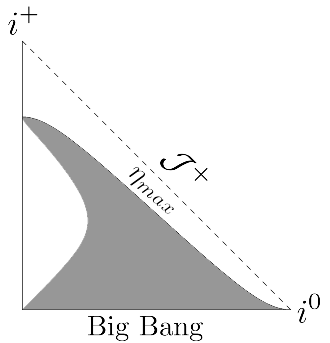
Figure 7: Penrose diagram for the model given by (28) with $m=1/2$, $n=-1$, $a_{0}=2$, $t_{s}=10$.

The Misner-Sharp horizon is on the left side of the grey region in Fig. 7 and it is timelike. The model initiates with Big Bang singularity and ends as $t\rightarrow t_{s}$, where $a\left(t_{s}\right)=$const., $\alpha\rightarrow\infty$, the density $\rho\rightarrow\infty$ and the pressure module $\left|p\right|\rightarrow\infty$. The future singularity displays behavior resembling the finite scale factor singularity (FSF) in the matter. Let us note that the models with $n=1/2$ and $n=-1$ give qualitatively the same future singularity for the matter sector but the behavior of $\alpha$ in both cases is different. In case of the models with $n>0$, as $t\rightarrow t_{s}$, the scalar field $\alpha\rightarrow 0$, resulting in the effective gravitational constant $G$ and the speed of gravitational interactions propagation $c$ approaching infinity. On the other hand, for $n<0$, as $t\rightarrow t_{s}$, $\alpha\rightarrow\infty$ which imply $G\rightarrow 0$ and $c\rightarrow 0$.

5 Conclusions

In this paper we employed a specific type of bimetric model with varying constants to explore the conformal structure of spacetimes using Penrose diagrams and to study singularities. We focused on the gravitational metric which describes the causal structure for the gravitational field. Our results indicate that for $n=1/2$, corresponding to a strong singularity according to Królak and Tipler’s definition, the nature of this singularity resembles that of the finite scale factor singularity (FSF). The Penrose diagrams exhibit similarities, although the Misner-Sharp horizon exhibits strong dependence on the initial parameters $a_{0}$ and $t_{s}$. We demonstrated that the behavior of the horizon depends on initial conditions and can be classified into three primary types. The nature of the Misner-Sharp horizon is almost identical for both $n=1/2$ and $n=3/2$. It is particularly intriguing that the result for $n=3/2$, which qualifies as a strong singularity according to Królak and Tipler’s definition, resembles the sudden future singularity (SFS), typically considered weak. Although parameters such as scale factor, density, and pressure align with SFS, the nature of the singularity differs. The singularity manifests at $\mathcal{J}^{+}$, as opposed to $\eta=$ const. in SFS. Moreover, the Misner-Sharp horizon differs from that in the SFS case. The conformal structure for $m=1/2$ and $n=-1$ is identical to that of the standard exotic singularity for the matter. In both cases the singularity emerges on hypersurface which is spacelike and the behaviour of Misner-Sharp horizon is timelike.

Our bimetric model assumes $\alpha\left(t\right)$ which can be interpreted as a scalar field. The dynamical gravitational constant and the dynamical speed of light in the gravitational metric depend on $\alpha$, preventing a clear separation between the effects of the dynamical gravitational constant and the dynamical speed of light.

Acknowledgments We wish to thank Mariusz Dabrowski for discussions.

References

- (1) Hawking S. W., Ellis G. F. R., 1973, The Large Scale Structure of Space-Time. Cambridge Univ. Press, Cambridge
- (2) J. Khoury, B. A. Ovrut, P. J. Steinhardt, and N. Turok, Ekpyrotic universe: Colliding branes and the origin of the hot big bang, Phys. Rev. D 64 (2001) 123522.
- (3) J. Khoury, B. A. Ovrut, N. Seiberg, P. J. Steinhardt, and N. Turok, From big crunch to big bang, Phys. Rev. D 65 (2002) 086007.
- (4) P. J. Steinhardt and N. Turok, Cosmic evolution in a cyclic universe, Phys. Rev. D 65 (2002) 126003.
- (5) P. J. Steinhardt and N. Turok, A Cyclic Model of the Universe, Science 296 (2002) 1436.
- (6) M. Gasperini and G. Veneziano, The pre-big bang scenario in string cosmology, Phys. Rep. 373 (2003) 1.
- (7) J.L. Tonry et al., Astroph. J. 594, 1 (2003); M. Tegmarket al., Phys. Rev. D69, 103501 (2004); R.A. Knop et al., Astrophys. J. 598, 102 (2003).
- (8) F. Tipler, Singularities in conformally flat spacetimes, Phys. Lett. A 64 (1977) 8.
- (9) A. Królak, Towards the proof of the cosmic censorship hypothesis, Class. Quantum Grav. 3 (1986) 267.
- (10) R. R. Caldwell, A phantom menace? Cosmological consequences of a dark energy component with super-negative equation of state, Phys. Lett. B 545 (2002) 23.
- (11) Da̧browski M. P., Stachowiak T., Szydłowski M., 2003, Phys. Rev. D, 68,103519
- (12) J.D. Barrow, Sudden future singularities, Class. Quantum Grav. 21 (2004) 79.
- (13) S. Nojiri and S. D.Odintsov, The final state and thermodynamics of dark energy universe, Phys.Rev. D 70 (2004) 103522.
- (14) M.P. Da̧browski and T. Denkiewicz Exotic-singularity-driven dark energy, AIP Conference Proceedings 1241 (2010) 561.
- (15) S. Nojiri, S. D. Odintsov and S. Tsujikawa, Properties of singularities in (phantom) dark energy universe, Phys.Rev. D 71 (2005) 063004.
- (16) M.P. Da̧browski and T. Denkiewicz Barotropic index w-singularities in cosmology, Phys. Rev. D 79 (2009) 063521.
- (17) P. H. Frampton, K. J. Ludwick and R. J. Scherrer The little rip, Phys. Rev. D 84 (2011) 063003.
- (18) P. H. Frampton, K. J. Ludwick and R. J. Scherrer Pseudo-rip: Cosmological models intermediate between the cosmological constant and the little rip, Phys. Rev. D 85 (2012) 083001.
- (19) H. Weyl, Ann. Phys., 59, 129 (1919).
- (20) A.S. Eddington, The Mathematical Theory of Relativity, Cambridge University Press, Cambridge, 1923.
- (21) New Pathways in Science, Cambridge University Press, Cambridge, 1934.
- (22) P.A.M. Dirac, Nature 139, 323 (1937).
- (23) Brans, C., and Dicke, R.H., Phys. Rev. 124 (1961), 925.
- (24) J.D. Barrow, Phys. Rev. D 59, 043515 (1999).
- (25) A. Albrecht and J. Magueijo, Phys. Rev. D 59, 043516 (1999).
- (26) J.D. Barrow and J. Magueijo, Class. Quantum Grav. 16, 1435.
- (27) J.D. Bekenstein, Fine-structure constant: Is it really a constant, Phys. Rev. D 25, 1527 (1982).
- (28) J.D. Bekenstein, Fine-structure constant variability, equivalence principle and cosmology, Phys. Rev. D 66, 123514 (2002).
- (29) M.P. Da̧browski and K. Marosek, Regularizing cosmological singularities by varying physical constants, JCAP 2013 (2013) 012.
- (30) K. Marosek and A. Balcerzak, Strength of singularities in varying constants theories, Eur. Phys. J.C (2019) 79 287.
- (31) Jacob D. Bekenstein, Relation between physical and gravitational geometry, Phys. Rev. D 48 (1993) 3641.
- (32) B. P. Abbott et al., Gravitational Waves and Gamma-Rays from a Binary Neutron Star Merger: GW170817 and GRB 170817A, ApJ 848 (2017) 13.
- (33) N. Cornish, D. Blas, and G. Nardini, Bounding the Speed of Gravity with Gravitational Wave Observations, Phys. Rev. Lett. 119 (2017) 161102.
- (34) J.D. Barrow, G.J. Galloway and F.J. Tipler, Sudden Future Singularities Mon. Not. Roy. Astr. Soc., 223 835 (1986).
- (35) Charles W. Misner and David H. Sharp, Relativistic Equations for Adiabatic, Spherically Symmetric Gravitational Collapse, Phys. Rev. 136 B571 (1964).
- (36) Tomohiro Harada, B. J. Carr, Takahisa Igata Complete conformal classification of the Friedmann-Lemaitre-Robertson-Walker solutions with a linear equation of state, Class. Quantum Grav. 35 105011 (2018).
- (37) M.P. Da̧browski and K. Marosek, Non-exotic conformal structure of weak exotic singularities Gen Relativ Gravit 50, 160 (2018).