Thermodynamically reversible quantum measurements and related work costs

Abstract

Considering a general microscopic model for quantum measurement comprising a measurement apparatus coupled to a thermal bath, we analyze the energetic resources necessary for the realisation of quantum measurements, including the process of switching on and off the coupling between the system and the apparatus, the transition to a statistical mixture, the classical readout, and the apparatus resetting. We show via general thermodynamic arguments that the minimal required work depends on the energy variation of the system being measured plus information-theoretic quantities characterizing the performance of the measurement – efficiency and completeness. Additionally, providing an explicit protocol, we show that it is possible to perform thermodynamically reversible measurement, thus reaching the minimal work expenditure. Finally, for finite-time measurement protocols, we illustrate the increasing work cost induced by rising entropy production inherent of finite-time thermodynamic processes. This highlights an emerging trade-off between velocity of the measurement and work cost, on top of a trade-off between efficiency of the measurement and work cost.

I Introduction

Quantum measurement, along with the stochastic evolution it triggers on the measured quantum system, stands as one of the most perplexing phenomena in quantum mechanics. On the one hand, the dynamics induced by quantum measurements is well-modeled, even when accounting for non-ideal, realistic measurement scenarios [1], and exhibit remarkable consistency with experimental observations. On the other hand, the underlying emergence of these dynamics from first principles [2] continues to be a subject of ongoing investigations [3, 4].

Moreover, during a measurement, both the entropy and energy of the measured system may undergo changes, rendering the measurement-induced dynamics akin to a thermodynamic transformation. This notion has led to the development of engines and refrigerators fueled by measurement-induced energy variations [5, 6, 7, 8, 9]. In a broader sense, quantum measurement represents a form of thermodynamic resource extending beyond the mere acquisition of information, which itself can be converted into work through protocols akin to Maxwell’s demons harnessing information from classical measurements.

Despite these thermodynamic analyses of quantum measurement, little is known about the actual energetic cost of realizing quantum measurements and how this relates with the energy received by the system. How closely do realistic quantum measurements approach fundamental limits? How can their energetic costs be optimized? These latter questions gain newfound significance as the energetic cost of implementing quantum algorithms, which typically necessitate numerous measurements for error correction, comes under scrutiny.

Pioneering studies [10, 11] already started to analyze those questions, including experimentally [12], and point at infinite energetic cost for ideal projective measurements [13], while an other study establishes that measurements of observables commuting with the free Hamiltonian of the system can be performed at no energetic cost [14]. The present study recovers the above results as particular situations.

More precisely, we present a framework for analyzing the energy expenditure associated with realistic nonideal quantum measurements. This framework is built upon a comprehensive microscopic model of a measurement apparatus, comprising a quantum meter, namely a quantum system interacting with the system of interest in order to encode the measurement outcome in its degrees of freedom, along with a thermal reservoir. The latter is responsible for the objectification [4, 14], a crucial stage of the measurement process during which the meter undergoes a transition to classical behavior, rendering the measurement outcome an objective fact. From the expression of the second law of thermodynamics within our model, we establish a general lower bound for the energy required to conduct quantum measurements. Remarkably, this bound aligns with an earlier finding by Sagawa and Ueda [15] regarding perfectly efficient measurements and extends their result to encompass arbitrary nonideal measurement scenarios. Our lower bound is composed of the energy absorbed by the measured system during the measurement, as well as of information-theoretic quantities that quantify the measurement quality through information acquired by the apparatus.

Through the analysis of a specific measurement protocol, we demonstrate the attainability of this lower bound. Key conditions for such attainability include quasi-static manipulation of the system-apparatus interaction (very slow relative to the thermalization timescale of the reservoir), as well as the full utilization of information acquired during the protocol. Moreover, we establish that a measurement of an observable commuting with the system’s Hamiltonian can be performed without expending any driving work in the quasi-static limit. Finally, for measurements conducted at finite speeds, the energy cost escalates due to increased entropy production (predominantly ”classical friction”). This gives rise to a dual trade-off between measurement duration, measurement efficiency, and energy expenditure.

    

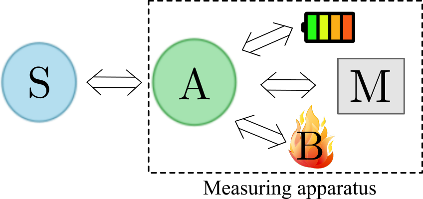
Figure 1: Up: Von Neumann chain model of the objectification process. Bottom: The model of measuring apparatus considered in this paper.

II Energetically closed model of quantum measurement

II.1 Modeling the objectification

In this section, we introduce and motivate our general model of measuring apparatus, used to draw conclusion about quantum measurement energetics. The measured system $S$, is assumed to be initially isolated in a state $\rho_{S}(0)$ with local Hamiltonian $H_{S}$. The aim of the operation is to measure an observable $Q_{S}$. Since $S$ is not directly accessible to the observer – the value of $Q_{S}$ cannot be read by just “looking” at it – standard measurement protocols [1] consider an auxiliary quantum system $A$ (which is a subpart of the total measuring apparatus) which is set to interact with $S$. As a consequence of the correlations established between $S$ and $A$ during their interaction, the state of $A$ contains information about $Q_{S}$. In a realistic measurement setup, this information is, at least partially, amplified and transferred to many other degrees of freedom until it reaches a macroscopic pointer, which can be directly read by the observer.

The redundant encoding of the measurement outcome in many degrees of freedom, a large part of which are inaccessible to observer is responsible for the irreversible nature of the measurement process, as pointed out in particular by the paradigm of quantum Darwinism [16]. The redundancy also makes the measurement outcome an objective reality, accessible by different observers, and is also crucial to prevent well-known paradoxes associated with the Wigner’s friend scenarios [17], which all incur from assuming an observer to have complete access to any information extracted from the system.

This process is sometimes called objectification [4, 14], and was first modeled by von Neumann by considering a second auxiliary system $A^{(1)}$ interacting with $A$ so as to acquire information about $Q_{S}$, followed by a third auxiliary system $A^{(2)}$ interacting with $A^{(1)}$, and so on, forming a macroscopic chain $A^{(1)}...A^{(N)}$ [1]. The chain can be stopped when the total system $SA^{(1)}...A^{(N)}$ behaves essentially classically, and the measurement outcome can be simply accessed by looking at the apparatus to find out its macroscopic state – a classical observation.

To bridge the gap with thermodynamics, we analyze here a slightly different model, where the role of the macroscopic chain of systems is played by a single quantum pointer $A$, together with a reservoir at thermal equilibrium $B$ and a classical memory $M$. In addition, a classical battery provides the work needed for the realization of the measurement (see Fig. 1b), and manifests itself in the form of time-dependent Hamiltonians.

The macroscopic reservoir $B$ ensures the objectification by inducing decoherence on the pointer: Namely, after interacting with the bath, if the decoherence process is complete, the state of the system $S$ and of the pointer $A$ is a fully incoherent mixture of perfectly distinguishable states associated with the different measurement outcomes. The distinguishable states corresponds to macrostates of the apparatus, in which the measurement outcome can be read by a mere classical information acquisition. In other words, once $B$ is explicitly included in the description, positioning the Heisenberg cut after the system $A$ is fully justified. In particular, reading the outcome in $A$ (or equivalently writing in down in classical memory $M$) does not trigger any additional exchange of energy and does not incur any energy cost, besides the cost to further process classical information [18]. This is an important property that makes our model energetically close, and allows us to perform an energy balance of the measurement beyond previous analyses of the measurement energetics [13, 14, 15].

II.2 Measurement protocol

We now present the protocol associated with a quantum measurement of $Q_{S}$. Before the measurement protocol starts, the global system $SAB$ starts in state $\rho_{S}(0)\otimes\rho_{AB}(0)$, that is, $A$ and $B$ are uncorrelated from $S$. To fully take into account any resource spent in the measurement process, we assume that $A$ and $B$ are initially at thermal equilibrium and weakly coupled such that $\rho_{AB}(0)=e^{-\beta(H_{A}+V_{AB}+H_{B})}/Z_{AB}\simeq e^{-\beta H_{A}}/Z_{A}\otimes e^{-\beta H_{B}}/Z_{B}$, where we ave introduced Hamiltonians $H_{A}$ and $H_{B}$ of $A$ and $B$ and (weak) coupling $V_{AB}$. Therefore, any non-equilibriumness in $A$ exploited during the measurement process is assumed to be prepared during next stages of the protocol.

The general protocol considered throughout the paper starts with a first step allowing the correlation of $S$ and $A$. During this step, the coupling between $S$ and $A$ is switched on, in presence of the decoherence induced by $B$. This is described by a global unitary evolution on $SAB$ for $t$ from $t_{0}$ to $t_{M}^{-}$,

$$U_{\text{on}}:={\cal T}\exp\left\{-i\int_{t_{0}}^{t_{M}^{-}}duH_{SAB}(u)\right\},$$ (1)

where the Hamiltonian of systems $S$, $A$, and $B$ is of the most general form

$$H_{SAB}(t)=H_{S}(t)+V_{SA}(t)+H_{A}(t)+H_{B}+V_{AB}(t),$$ (2)

(assuming no control over the bath $B$) and where ${\cal T}\exp$ denotes the time-ordered exponential.

As mentioned in previous section II.1, in order to model a complete measurement setup, up to a level where the Heisenberg cut is justified, we impose that, at the end of this step (denoted time $t_{M}$), the state of $SA$ is an incoherent mixture of the orthogonal states that will be associated with different measurement outcomes. We therefore write:

$$\rho_{SA}(t_{M}):={\rm Tr}_{B}[U_{\text{on}}\rho_{S}(0)\rho_{AB}(0)U_{\text{on}}^{\dagger}]=\sum_{r}p_{r}\rho_{SA|_{r}}(t_{M}),$$ (3)

with

$$\text{Tr}\{\rho_{A|_{r}}(t_{M})\rho_{A|_{r}^{\prime}}(t_{M})\}=\delta_{rr^{\prime}}\text{Tr}\{\rho_{A|_{r}}^{2}(t_{M})\}.$$ (4)

The latter orthogonality condition ensures that the states $\rho_{A|_{r}}(t_{M})$ are fully distinguishable and therefore behave as macroscopically different classical states: this can be understood as a condition for classicality of the final state of the apparatus. More precisely, $\rho_{SA|r}(t_{M})$ (resp. $\rho_{A|r}(t_{M})=\text{Tr}_{S}\{\rho_{SA|r}(t_{M})\}$) corresponds to the state of $SA$ (resp. of $A$) obtained during the classical observation of $A$, which selects a particular element $r$ of the statistical mixture with probability $p_{r}$. The aim of a measurement is generally to generate a probability distribution $p_{r}$ which is correlated to the distribution of the eigenvalues of the observable $Q_{S}$ in the initial state of $S$, thereby acquiring information about the value of $Q_{S}$.

To avoid any issue associated to interpretations of quantum mechanics, we formally represent the operation of reading the measurement outcome in the apparatus via a reversible operation correlating each orthogonal state $\rho_{A|_{r}}(t_{M})$ into a distinct state of a classical memory system $M$, that we represent in terms of density operators $|r\rangle_{M}\langle{r}|$ for simplicity. The memory is assumed to be initially in a pure reference state $|{\text{ref}}\rangle_{M}\langle{\text{ref}}|$, and its free dynamics is assumed to be negligible over the duration of the measurement protocol (for instance, fully degenerate Hamiltonian). After the reading process (time $t_{M}^{+}$), the correlated state of $SA$ and $M$ is therefore:

$$\rho_{SAM}(t_{M}^{+})=\sum_{r}p_{r}\rho_{SA|_{r}}(t_{M})\otimes|r\rangle_{M}\langle r|.$$ (5)

This correlation can be done perfectly in principle owing to the orthogonality of the $\rho_{A|_{r}}(t_{M})$ states, and at no work cost for a degenerate memory Hamiltonian. While (classical) errors coming from imperfect encoding in the memory could be analyzed, we choose to focus on limitations of the measurement quality coming from the interaction between $S$, $A$ and $B$.

To reinitialize the apparatus, two additional steps are needed. First, if the $S-A$ coupling was not off at the end of the first driving phase, it must be switched off, which is described by another global unitary on $SAB$ for $t$ from $t_{M}^{+}$ to $t_{F}$,

$$U_{\text{off}}:={\cal T}\exp\left\{-i\int_{t_{M}^{+}}^{t_{F}}duH_{SAB}(u)\right\}.$$ (6)

We also assume that $B$ has returned to equilibrium before this switching off process begins (or equivalently that the switching off process involves another thermal reservoir). At the end of this step, the correlated state of the system, apparatus and memory reads:

$$\rho_{SAM}(t_{F})=\sum_{r}p_{r}\rho_{SA|r}(t_{F})\otimes|r\rangle_{M}\langle r|$$ (7)

with, $\rho_{SA|r}(t_{F})={\rm Tr}_{B}[U_{\text{off}}\rho_{SA|r}(t_{M})\otimes\rho_{B}(0)U_{\text{off}}^{\dagger}]$.

Second, the system $AM$ must be reset to its initial state. In particular, the memory $M$ must be erased (potentially after its content has been used e.g. to design feedback operation).

When outcome $r$ is obtained, the conditional final state of the system can generically be cast under the form (see Appendix A):

$$\rho_{S|r}(t_{F})=\frac{1}{p_{r}}\sum_{s}M_{r,s}\rho_{S}(0)M_{r,s}^{\dagger},$$ (8)

where we have introduced the Kraus operators $M_{r,s}\propto{}_{B}\langle i^{\prime}|{}_{A}\langle m^{\prime}|U_{\text{on}}\Pi_{r}^{A}U_{\text{off}}|m\rangle_{A}|i\rangle_{B}$ verifying $\sum_{r,s}M_{r,s}^{\dagger}M_{r,s}=\mathds{1}$. Note that $s$ is a collective index gathering all sets $(n,i,n^{\prime},i^{\prime})$ of initial and final states of $A$ and $B$ yielding system operators ${}_{B}\langle n^{\prime}|{}_{A}\langle i^{\prime}|U_{\text{on}}\Pi_{r}^{A}U_{\text{off}}|n\rangle_{A}|i\rangle_{B}$ which are proportional to each other – where $\{|n\rangle_{A}\}$ and $\{|i\rangle_{B}\}$ are bases of the Hilbert spaces of $A$ and $B$, respectively. Additionally, the projective operator $\Pi_{r}^{A}$ is the projector onto the support of $\rho_{A|r}(t_{M})$. The quality of the measurement process can be related to the properties of the states $\{\rho_{S|r}(t_{F})\}_{r}$ [1]. The textbook case of a projecting measurement, such that $\rho_{S|r}(t_{F})\propto\pi_{r}^{S}\rho_{S}(t_{0})\pi_{r}^{S}$, with $\pi_{r}^{S}$ some projective operator of $S$, is a limiting case expected to be reached only at infinite resource cost [13]. By contrast, realistic measurement models can yield to measurement that are invasive (the statistics of the measurement observable in the average post-measurement state $\sum_{r}p_{r}\rho_{S|r}(t_{F}))$ is different from the statistics prior to the measurement), partially inefficient (a fraction of the information leaking in the environment is not available in the memory, such that the post-measurement state can be a mixed state) and incomplete (such as weak measurements [19] which only partially evolve the system’s state towards an eigenstate of the measured observable).

In the remainder of this paper, we derive a lower bound on the work required to perform such realistic measurement protocols. Such lower bound depends on the quality of the measurement. It is then followed by some illustrative situations and protocols, where it is also possible to study additional energetic cost induced by irreversible finite-time protocols.

III General thermodynamic argument

III.1 A lower bound on the work cost of the measurement process

In this section, we use quantum formulations of thermodynamic laws to derive a lower bound on the work expenditures during the measurement process. The lower bound, which depends on the properties of the measurement, takes the form:

$$W_{\text{dr}}+W_{\text{reset}}\geq\Delta E_{S}+\frac{1}{\beta}\left(J_{S}+\left\langle I_{S:A}\right\rangle\right).$$ (9)

On the left-hand side, $W_{\text{dr}}$ is the work cost to drive the system and apparatus through the measurement process, while $W_{\text{reset}}$ is the work cost to reset the apparatus and memory to their initial state. The right-hand side is the sum of three terms which depends on the measurement properties. First, $\Delta E_{S}=\text{Tr}\{H_{S}\left(\rho_{S}(t_{F})-\rho_{S}(0)\right)\}$ is the average energy variation of the measured system. This term vanishes for measurements of an observable $Q_{S}$ which commutes with the Hamiltonian of the system. Such measurements can be made noninvasive and verify $[M_{r,s},H_{S}]=0$.

Second,

$$J_{S}=\sum_{r}p_{r}\left(S[\rho_{S}(t_{0})]-S[\rho_{S|r}(t_{F})]\right),$$ (10)

with $S[\rho]=-\text{Tr}\{\rho\log\rho\}$ the Von Neumann entropy of state $\rho$, quantifies the average information obtained on the system state during each single run of the measurement protocols (each corresponding to a different measurement outcomes $r$). This quantity verifies $J_{S}\in\big{[}S[\rho_{S}(t_{0})]-\ln d_{s};S[\rho_{S}(t_{0})]\big{]}$. As we detail below, it may be negative for inefficient measurements (where only a fraction of the information leaking from $S$ is accessible to the observer).

Finally,

$$\left\langle I_{S:A}\right\rangle=\sum_{r}p_{r}\left(S[\rho_{S|r}(t_{F})]+S[\rho_{A|r}(t_{F})]-S[\rho_{SA|r}(t_{F})]\right),$$ (11)

is the average residual mutual information at $t_{F}$ between $S$ and $A$. It quantifies information about $S$ transferred to $A$ but not to the memory for it is encoded in inaccessible degrees of freedoms of the pointer. It is therefore one possible source of measurement inefficiency.

Eq. (9) is the main result of this section. It relates the measurement work cost with the energy change of the system and information-theoretic quantities which depend on the measurement performances (in particular its efficiency and its strength as detailed below). Eq. (9) becomes an equality when the whole protocol is performed in a reversible way, which requires quasi-static drives allowing equilibration between $SA$ and $B$ at all times, but also to fully exploit all the information obtained about the states of $S$ and $A$. We will come back with more details on this point in Section IV.4.

III.2 Proof of the lower bound

In this section, we derive Eq. (9). To do so, we first gather the evolution of the total system $SAMB$ from time $t_{0}$ to $t_{F}$ in a single unitary $U=U_{\text{off}}U_{\text{reg}}U_{\text{on}}$ which is all-in-all generated by an Hamiltonian of the form $H(t)=H_{SA}(t)+H_{B}+V_{AB}+V_{AM}(t)$, where $V_{AM}(t)$ describes without loss of generality the encoding of the measurement outcome in $M$ mentioned in section II.2, which is also denoted by unitary $U_{\text{reg}}$. We then use the formalism from Ref. [20] to express the entropy production associated with the measurement protocol.

From [20], the first law implies that work performed on the total system $SAMB$ when varying in time Hamiltonian $H(t)$ is equal to its total energy variation:

$$W_{\text{dr}} = \left\langle H(t_{F})\right\rangle-\left\langle H(t_{0})\right\rangle$$ (12)

$$= \Delta E_{SA}+\Delta\left\langle V_{AB}\right\rangle+\Delta E_{B},$$

where $\Delta X=X(t_{F})-X(t_{0})$ refers to a variation of the average quantity $X$ between times $t_{F}$ and $t_{0}$, while $E_{\alpha}(t)=\left\langle H_{\alpha}(t)\right\rangle$ denotes the internal energy of system $\alpha$ at time $t$. The associated expression of the second law for the transformation of system $SAM$ in contact with $B$ reads:

$$\sigma=\Delta S_{SAM}-\beta Q_{B}\geq 0$$ (13)

with $\sigma$ the total entropy produced, and $Q_{B}=-\Delta E_{B}$ the average heat flow exchanged with the bath $B$. In all the article, $S_{\alpha}(t)=S[\rho_{\alpha}(t)]$ denotes the Von Neumanm entropy of system $\alpha$ at time $t$. Combining these two laws leads to:

$$W_{\text{dr}} \geq \Delta E_{SA}+\Delta\left\langle V_{AB}\right\rangle-\frac{1}{\beta}\Delta S_{SAM},$$ (14)

On the other hand, the work cost to reset systems $A$ and $M$ is lower-bounded by the associated variation of free energy:

$$W_{\text{reset}} \geq F_{AM}(t_{0})-F_{AM}(t_{F})=-\Delta E_{A}+\frac{1}{\beta}\Delta S_{AM},$$

(15)

remembering that we considered a memory register $M$ with a fully degenerate Hamiltonian. We now sum up both inequalities and use the assumption $V_{SA}(t_{F})=V_{SA}(t_{0})=0$, such that $\Delta E_{SA}=\Delta E_{S}+\Delta E_{A}$. Neglecting the apparatus-bath coupling energy $\Delta\left\langle V_{AB}\right\rangle$, we obtain:

$$W_{\text{dr}}+W_{\text{reset}} \geq \Delta F_{S}+\frac{1}{\beta}I(S:AM).$$ (16)

That is, the work cost is lower bounded by the sum of the change in the free energy of system $S$, $\Delta F_{S}=\Delta E_{S}-(1/\beta)\Delta S_{S}$ and $1/\beta$ times the mutual information $I(S:AM)=\Delta S_{S}+\Delta S_{AM}-\Delta S_{SAM}$ between the system and the apparatus.

To further simplify this bound and obtain Eq. (9), we finally inject the specific form Eq. (7) of the conditional states, noting that $\Delta S_{SAM}=\sum_{r}p_{r}S[\rho_{SA|r}(t_{F})]+{\cal H}(\{p_{r}\})-S_{A}(t_{0})-S_{S}(t_{0})$, with

$${\cal H}(\{p_{r}\})=-\sum_{r}p_{r}\log p_{r},$$ (17)

the Shannon entropy of the measurement outcome distribution $p_{r}$.

III.3 Efficient measurements

To compare with earlier results [15, 21] and further interpret Eq. (9), we first focus on the case of efficient measurements, which are such that all the information acquired about the system can be transferred to the memory $M$. Mathematically, efficient measurements lead to a conditional state of $S$ associated with measurement outcome $r$ obtained from the application of a single Kraus operator $M_{r}$ on the initial system state:

$$\rho_{S|r}(t_{F})=\frac{M_{r}\rho_{S}(t_{0})M_{r}^{\dagger}}{p_{r}},$$ (18)

with $\sum_{r}M_{r}^{\dagger}M_{r}=\mathds{1}$ and $p_{r}=\text{Tr}\{M_{r}^{\dagger}M_{r}\rho_{S}(t_{0})\}$. Such measurement therefore prepare pure conditional states from pure initial states. Depending on the interaction strength between the $S$ and $A$, the measurement can be complete [1] – that is, $\rho_{S|r}(t_{F})$ is independent on the initial state, as it is the case for a projective/strong measurement where $M_{r}$ is a projector onto an eigenstate of the measured observable – or incomplete, such as weak measurements [19].

As we show in Appendix A, the condition of efficient measurement implies that $\left\langle I_{S:A}\right\rangle=0$. Indeed, a non-zero mutual information between $S$ and $A$ in the conditional states $\rho_{S|r}(t_{F})$ reveals the existence of information on $S$ stored in A but not transferred to M, hence a loss of efficiency of the measurement.

In addition, for an efficient measurement, $J_{S}$ becomes equal to the so-called quantum-classical mutual information between $S$ and the measurement outcomes [22], defined as:

$$I_{\text{QC}}=S_{S}(t_{0})-\sum_{r}p_{r}S\left[\frac{\sqrt{E_{r}}\rho_{S}(t_{0})\sqrt{E_{r}}}{p_{r}}\right]$$ (19)

with $E_{r}$ the effect operator defined from $p_{r}=\text{Tr}\{E_{r}\rho_{S}(t_{0})\}$. Our bound Eq. (9) therefore coincides with the result of [15, 21] in the regime where the latter was derived, i.e. for efficient mesurements.

The quantity $I_{\text{QC}}$ verifies [22, 23]

$$0\leq I_{\text{QC}}\leq{\cal H}(\{p_{r}\}).$$ (20)

The limit $I_{\text{QC}}\to 0$ corresponds to a weak measurement acquiring an infinitesimal amount of information [19].

An important consequence is that efficient measurements fulfill $J_{S}\geq 0$, i.e. always lead to an increased knowledge of the system’s state. The bound Eq. (9) implies that work must be spent beyond the energy received by the system to perform the measurement.

A projective measurement associated with Kraus operators which are rank-1 projectors fulfils $I_{\text{QC}}=S_{S}(t_{0})$ and therefore saturates the upper bound ${\cal H}(\{p_{r}\})$ of Eq. (20) when the initial state is a mixture of the eigenstates of the measured observable. Note that according to our lower bound Eq. (9), it is in principle possible to realize a projective measurement at finite energetic cost, apparently conflicting the results in [13]. We will see in Section IV that the key to the resolution of this apparent contradiction is to take into account finite-time dynamics which unavoidably brings additional costs.

III.4 General case: possibly inefficient measurements

Our results also apply to the broader case of measurement with finite detection efficiency, i.e. the more realistic case where a fraction of the information extracted from the system leaks into inaccessible degrees of freedoms in the environment. In this case, the conditional state of the system can generically be cast under the form:

$$\rho_{S|r}(t_{F})=\frac{1}{p_{r}}\sum_{s}M_{rs}\rho_{S}(t_{0})M_{rs}^{\dagger},$$ (21)

with $\sum_{r,s}M_{rs}^{\dagger}M_{rs}=\mathds{1}$. In this general regime, the different contributions $J_{S}$, $\left\langle I_{S:A}\right\rangle$ and $\Delta E_{S}$ are related to qualitatively different properties of the measurement:

• $J_{S}$ quantifies the net average information gain during the measurement. In the case of inefficient measurement, this quantity does not coincide with the quantum-classical mutual information, and can be negative (which means that the measurement is so inefficient that the state’s entropy of each conditional state is larger than the initial entropy [24]). While $J_{S}<0$ implies a lower work cost for the measurement process, it corresponds to cases where information is lost, so a measurement process consuming information about the system. A particular case of protocol verifying $J_{S}<0$ is the combination of an efficient measurement with a protocol converting information about the initial state into extracted work (i.e. a Maxwell Demon/Szilard engine protocol), which indeed enables one to reach lower net work costs (see also Appendix C.2). It is useful to rewrite $J_{S}=\xi_{S}-\Delta S_{S}$, with

  $$\xi_{S}=S_{S}(t_{F})-\sum_{r}p_{r}S[\rho_{S|r}(t_{F})],$$ (22)

  the Holevo information [25] about the outcome $r$ in the state $\rho_{S}(t_{F})=\sum_{r}p_{r}\rho_{S|r}(t_{F})$.

• $\xi_{S}\in[0;{\cal H}(\{p_{r}\})]$ quantifies how well the states $\rho_{S|r}(t_{F})$ can be distinguished from each other, and therefore the average gain of information about the final system state obtained when reading the measurement outcome versus not reading it. It therefore quantifies the efficiency of the measurement (and goes to zero with the efficiency see Section IV.2). We therefore see that the efficiency of the measurement is associated with larger work costs.

• $\log d_{S}\leq-\Delta S\leq 0$ is the average information loss about the system state when measurement outcome is ignored, and therefore only provides information about the strength of the measurement. Note that it depends on the initial state of the system, and can be zero (for instance for a system initially in a mixture of eigenstates of the measured obervable). In contrast, it reaches maximum value $\log d_{S}$, with $d_{S}$ the dimension of the Hilbert space of $S$, for a pure initial state transformed into a mixture of measurement observable eigenstates by the measurement process (when the outcomes are not read).

• $\left\langle I_{S:A}\right\rangle$ is associated to one possible source of inefficiency for the measurement, that is the possibility to lose information inside the measuring apparatus due to the coarseness of the reading procedure (i.e. the rank of the projectors $\Pi_{A,r}$). We see that this coarse-graining tends to reduce the amount of information available from the measurement outcome quantified by $J_{S}$, but also tends to increases the term $\left\langle I_{S:A}\right\rangle$, leaving the measurement cost constant. In other words, the latter is determined by the total amount of extracted information, whether it is stored in accessible degrees of freedom or not. Note that the switching off process can also erase remaining correlations between $S$ and $A$, so that one can have $\left\langle I_{S:A}\right\rangle=0$ even though some information remained in $A$ after the observation. This irreversible information loss in the environment then leads to an increased entropy production, and therefore still increases the work cost (see Section IV.4 for an illustration of this phenomenon).

• $\Delta E_{S}$ corresponds to energy exchanged directly between the system and the apparatus. This quantity is only non-zero when the measured observable does not commute with the system’s Hamiltonian. In such cases, $\Delta E_{S}$ can be positive or negative depending on the initial system state. When the system receives energy from the measuring apparatus ($\Delta E_{S}\geq 0$), the lower bound Eq. (9) is increased by the same amount. This mechanism lies at the basis of measurement-driven engines [7, 6, 26, 27] which convert into work this same energy gained by the system via the measurement. One of the insights brought by our results is therefore to identify precisely the source of this energy gained by the system in a large class of models of measuring apparatuses. The lower bound on the measurement work cost Eq. (9) can be used to upper bound the efficiency of such engines when seen as work-to-work transducers. In contrast, the case $\Delta E_{S}\leq 0$ corresponds to a decrease in the lower bound Eq. (9). Once again, measurement-driven engines and their ability to convert into work the energy received by the system during a measurement [7], provide examples where the energy extracted from the system indeed corresponds to a decrease of the net work cost.

Our inequality Eq. (9) therefore provides a general lower bound which can be applied to diverse situations of interest. In the remainder of the paper, we consider more specific measurement protocols, allowing us to test the validity of this lower bound, show its tightness and investigate additional work expenditure related to finite-time measurements.

IV Reaching the minimum work cost: case of a measurement of an observable which commutes with the Hamiltonian

In this section, we analyze how a class of measurement protocols associated with measurement observables which commute with the system’s Hamiltonian (i.e. quantum non-demolition measurements [28]) can saturate the bound Eq. (9). As large driving cost are expected to be obtained if $A$ is driven far from equilibrium with $B$, we investigate measurement protocols where only the coupling $V_{SA}$ between the system and the apparatus is varied, having in mind that a quasi-static variation of $V_{SA}$ should lead to a reversible process which may saturate the lower bound.

IV.1 Measurement from the variation of the system-meter coupling

We specify the general protocol introduced in section II.1 in two ways: First, we consider that only the coupling term $V_{SA}(t)$ in $H_{SAB}(t)$ is time dependent, and that it is of the form

$$V_{SA}(t)=\chi(t)Q_{S}\,R_{A},$$ (23)

where $Q_{S}$ is an observable of the system (the one being measured), $R_{A}$ an observable of the apparatus and $\chi(t)$ a time dependent coupling strength. We consider that $\chi(0)=\chi(t_{F})=0$, and denote $\chi(t_{M})=\chi_{M}$, the coupling strength at the time where the meter is read. The system Hamiltonian is time-independent $H_{S}=\sum_{k=1}^{d_{S}}e_{k}\pi_{k}^{S}$, with $\pi_{k}^{S}$ the projector onto the $k$th energy eigenstate. In this section, we focus on observables $Q_{S}$ fulfilling $[Q_{S},H_{S}]=0$. We further assume $[R_{A},H_{A}]=0$, a condition which is fulfilled by some (but not all) experimental protocols and enables to draw simple analytical conclusions.

Second, we consider a bosonic bath of Hamiltonian $H_{B}=\sum_{j}\omega_{j}b_{j}^{\dagger}b_{j}$, coupled to $A$ via Hamiltonian $V_{AB}=AB$ where $A$ is an arbitrary operator of $A$ which does not commute with $R_{A}$ nor $H_{A}$, and $B=\sum_{j}g_{j}(b_{j}^{{\dagger}}+b_{j})$ is a bosonic bath operator. In the weak system-bath coupling limit, we can describe the dynamics of $S$ and $A$ during the switching processes via a Bloch-Redfield master equation (that we derive for arbitrary systems $S$ and $A$ in Appendix D). We consider for simplicity that $\chi(t)$ is varied on a time-scale much longer than the correlation time $\tau_{c}$ of the bath, leading to time-dependent system transition frequencies, and therefore time-dependent dissipation rates. The obtained master equation induces relaxation at rates dependent on the measurement outcome. For a given value of the coupling constant $\chi_{M}$, its steady state is diagonal in the eigenbasis of system $S$, i.e. it takes the form (see Appendix E):

$$\rho_{SA}^{\rm ss}:=\sum_{k=1}^{d_{S}}p_{k}(0)\pi_{k}^{S}\otimes\rho_{A,k}^{\rm th},$$ (24)

where

$$\rho_{A,k}^{\rm th}=\frac{1}{Z_{A,k}}e^{-\beta H_{A,k}},$$ (25)

is the thermal equilibrium state of $A$ when $S$ is initially in the $k$th energy eigenstate, with $Z_{A,k}={\rm Tr}[e^{-\beta H_{A,k}}]$, $H_{A,k}=\sum_{n}E_{n,k}\pi_{n}^{A}$ and $E_{n,k}:=E_{n}+\chi_{M}q_{k}r_{n}$. Moreover, $\pi_{n}^{A}$ is the projector onto the $n$th energy level of $H_{A}$, associated with energy $E_{n}$, and $r_{n}$ is the $n$th eigenvalue of $R_{A}$.
This state is not yet in the form of Eq. (3) (the states $\rho_{A,k}$ are not orthogonal), but can be easily written in such form because each $\rho_{A,k}$ is diagonal in the basis $\{|n\rangle\}$. To do so, we consider that each measurement outcome $r$ is associated with a subspace ${\cal H}_{r}$ spanned by a subset $\{|n\rangle,n\in{\cal N}_{r}\}$ of the energy eigenstates of $A$. In more operational terms, this means that a function of the energy of $A$ is read with a finite resolution. We then identify

$$\rho_{SA|r}=\frac{1}{p_{r}}\sum_{k=1}^{d_{S}}p_{k}(0)\pi_{k}^{S}\otimes\Pi^{A}_{r}\rho_{A,k}\Pi_{r}^{A},$$ (26)

with $\Pi_{r}^{A}$ the projector onto subspace ${\cal H}_{r}$. Thus, the steady-state of $SA$ in presence of a non-zero coupling satisfies our assumption (3) for a measurement process. We can therefore consider the following protocol: (i) $A$ is initially in the equilibrium state $\rho_{A}(0)=e^{-\beta H_{A}}/Z_{A}$; (ii) The coupling $\chi(t)$ is increased from $0$ to $\chi_{M}$, and then kept constant for a time long enough to reach the steady state associated to $\chi_{M}$ and ensure that $SA$ is in a classical mixture of the different $\rho_{SA|r}$; (iii) At time $t_{M}$, the result is read and encoded in the memory $M$ which was initially in a reference pure state; (iv) The coupling is decreased up to $\chi(t)=0$ and kept constant until $A$ thermalizes back to $\rho_{A}(0)$; (v) After the result has been potentially used for feedback operations, the memory is reset to a reference pure state.

At the final time $t_{F}$ of the protocol, the system and meter are in the state:

$$\rho_{SA|r}=\rho_{S|r}(t_{F})\otimes\rho_{A}(0).$$ (27)

with

$$\rho_{S|r}(t_{F})=\frac{1}{p_{r}}\sum_{k=1}^{d_{S}}Tr\{\Pi_{r}^{A}\rho_{A,k}\}p_{k}(0)\pi_{k}^{S}.$$ (28)

IV.2 Measurement quality and lower bound

Due to the form of the final state, we have $\left\langle I(S:A)\right\rangle=0$ (the final state has a factorized form). In addition, $\Delta E_{S}=0$ as the measured observable commutes with the system Hamiltonian. For this class of protocols, we therefore have:

$$W_{\text{drive}}+W_{\text{reset}}\geq\frac{1}{\beta}J_{S}.$$ (29)

We see in Eq. (28) that the average system state at time $t_{F}$ is $\rho_{S}(t_{F})=\sum_{k=1}^{d_{S}}p_{k}(0)\pi_{k}^{S}$ for any value of $\chi_{M}>0$. That is, the measurement always fully projects the system in the eigenbasis of the observable (it has maximal strength). In contrast, $\chi_{M}$ controls the efficiency of the measurement which can be quantified by $\eta=1+(J_{S}-S_{S}(0))/\ln d_{S}$ which reaches $1$ ($0$) when the states $\rho_{S|r}$ are pure (have maximal entropy $\ln d_{S}$). From Eq. (28), we simplify the information gain $J_{S}$ about the system as:

$$J_{S}=S_{S}(0)+\mathcal{H}[\{p_{r}\}]-\mathcal{H}[\{p_{k,r}\}],$$ (30)

where $\mathcal{H}[\{p_{i}\}]=-\sum_{i}p_{i}\ln p_{i}$ is Shannon’s entropy of distribution $\{p_{i}\}$. It is also insightful to express the information gain as $J_{S}=I[p_{k}(0):p_{r}]-\Delta S_{S}$, where $I[p_{k}(0):p_{r}]$ is the mutual information between the distribution $\{p_{k}(0)\}$ which describes how the eigenvalues of $Q_{S}$ are distributed in the initial state, and the distribution $p_{r}$, which is the measured distribution.

To relate the efficiency of the measurement to the parameters of the model, we analyze the case where the system is a qubit of Hamiltonian $\frac{\omega_{S}}{2}\sigma_{z}$, with $\sigma_{z}=|e\rangle\langle e|-|g\rangle\langle g|$ and system $A$ is an oscillator of Hamiltonian $\omega_{c}a^{\dagger}a$. Moreover, we split the oscillator space in two by introducing the energy threshold $n_{s}$ and by defining the projectors $\Pi_{r=\pm}^{A}$ as $\Pi_{+}^{A}=\sum_{n\leq n_{s}}|n\rangle_{A}\langle n|$ and $\Pi_{-}^{A}=\sum_{n>n_{s}}|n\rangle_{A}\langle n|$. The efficiency $\eta$ is plotted in Fig. 2. From panels 2a) and b), it is clear that $J_{S}$ is maximized for a finite value of the inverse temperature $\beta$ which depends on the choice of energy threshold $n_{s}$. When $n_{s}$ and $\beta$ are scaled accordingly, the curves collapse on a unique function of $\chi_{M}$ as shown in Fig.2c). Then, the limit of an efficient measurement is reached asymptotically for $\chi_{M}\to\omega_{c}$.

Figure 2: Efficiency $\eta=1+(J_{S}-S_{S}(0)/\log 2$ of the measurement as a function of $\beta\omega_{c}$ for the energy threshold $n_{s}=0$ (a) and $n_{s}=10$ (b). The blue solid, red dashed and green dotted curves correspond to $\chi_{M}/\omega_{c}=0.3$, $0.7$ and $0.99$, respectively. (c): Efficiency $\eta$ as a function of $\chi_{M}/\omega_{c}$ for $(n_{s},\beta\omega_{c})=(100,0.03)$ (solid blue) and $(n_{s},\beta\omega_{c})=(0,3)$ (dashed orange).

IV.3 Quasi-static limit and finite-time-induced costs

We first analyze the work $W_{\text{drive}}$ associated with the variation of the system’s Hamiltonian over the entire protocol (where the $S-A$ coupling is switched on and off). Neglecting the work to record the measurement outcome in the classical memory (e.g. assumed to have a degenerate Hamiltonian), the total work spent to switch on and off the coupling between the system and the apparatus can be computed from:

$$W_{\text{dr}} = \int_{0}^{t_{F}}dt{\rm Tr}\left[\rho_{SAB}(t)\frac{d}{dt}H_{SAB}(t)\right]$$ (31)

$$= \int_{0}^{t_{F}}dt\dot{\chi}(t){\rm Tr}_{SA}\left[\rho_{SA}(t)Q_{S}R_{A}\right].$$

In appendix C.1, we show that in the quasi-static limit where the apparatus is at any time in one of the thermal states $\rho_{A,k}(t)$ conditioned to the system being in state $|k\rangle_{S}$, the work cost $W_{\text{drive}}$ vanishes, that is:

$$\underset{t_{f}\to\infty}{\lim}W_{\text{dr}}=0.$$ (32)

We further analyze the behavior in finite time and how the adiabatic limit is reached on the qubit and oscillator case introduced in the previous section. For such system, the adiabatic limit corresponds to $\dot{\chi}/\kappa\ll\chi_{M}$ (equivalent to $\kappa t_{M}\gg 1$), where $\kappa$ corresponds to the dissipation rate induced by the bath. In Appendix C.3, we compute the first non-zero correction to the adiabatic work cost, which is a function of the ratio $\dot{\chi}/\kappa$ and of the initial qubit population $p_{e}(0)=\langle e|\rho_{S}(0)|e\rangle$. We plot the two extreme values $W_{\text{drive}}^{\pm}$ (associated with $p_{e}(0)=1,0$) in Fig. 3. We observe that the adiabatic limit is more easily reached at small temperature and that both the fluctuations of the work cost and the average work cost can diverge for large values of $\chi_{M}\lesssim\omega_{c}$. As seen in Fig.  2, an efficient measurement is obtained in the limit $\chi_{f}\rightarrow\omega_{c}$, which in this model results in a diverging work cost. As projective measurements constitute a subfamily of efficient measurement, we recover the diverging work cost pointed out in [13].

In summary, we observe here a double trade-off between the efficiency of the measurement, the duration of the measurement and the work cost: Both decreasing the duration and increasing the efficiency require larger more work.

Figure 3: First nonadiabatic correction to the driving work cost $W_{\text{drive}}^{(1)}$ in the case where $S$ is a qubit and $A$ an oscillator. Blue (Orange) curves correspond to the case where the qubit is initially state $|e\rangle$ ($|g\rangle)$. a) As a function of the maximum coupling strength $\chi_{M}$ (at fixed coupling switching rate $\dot{\chi}$), b) As a function of the inverse temperature $\beta$, c) As a function of the time length $\tau_{\text{M}}=\chi_{M}/\dot{\chi}$ taken to switch on the coupling (at fixed final coupling strength $\chi_{M}$).

IV.4 Reversible measurement protocol

In this section, we explain how the quantum measurement can be performed as a reversible thermodynamic process, thereby reaching the minimum work cost. We have shown that in the adiabatic limit, that driving work $W_{\text{drive}}$ vanishes while the total work cost $W_{\text{drive}}+W_{\text{reset}}$ does not saturate the lower bound Eq. (9). This behavior signals additional sources of entropy production which are present even for quasi-static variations of the coupling. We identified two origins for this extra irreversibility (see Appendix C.2). The first one, $\sigma_{S}$, corresponds to the entropy increase of the average qubit state due to the projection in the measurement basis, and is equal to

$$\sigma_{S}={\cal H}(\{p_{k}(0)\})-S_{S}(0).$$ (33)

This term fulfils a fluctuation theorem and was identified as the entropy production associated with the measurement in previous works [29]. The second contribution is the entropy production associated with the thermalization of the meter $A$ after the measurement result has been read. It is equal to

$$\sigma_{A} = D[\rho_{SA|r}(t_{M}^{+})|\rho_{SA|r}^{\text{th}}]$$ (34)

$$= {\cal H}(\{p_{k,r}\})-{\cal H}(\{p_{k}(0)\}).$$

and is due to the nonequilibrium nature of the state $\rho_{SA|r}(t_{M}^{+})$ (obeying to Eq. (3)), even in the quasi-static limit. In the quasi-static limit (but still at finite speed), such out-of-equilibrium state irreversibly relaxes to $\rho_{SA|r}^{\text{th}}=\frac{1}{p_{r}}\sum_{k}p_{k,r}\pi_{k}^{S}\otimes\rho_{A,k}^{\text{th}}$ before the coupling is significantly modified to be switched off, yielding to non-zero value of $\sigma_{A}$.

All in all, the total work cost is equal to the lower bound $J_{S}/\beta$ plus three sources of entropy production,

$$W_{\text{drive}}+W_{\text{reset}}^{\text{rev}}=\frac{1}{\beta}(\sigma_{\text{drive}}+\sigma_{S}+\sigma_{A})+\frac{1}{\beta}J_{S}.$$ (35)

As commented above, the first source of entropy production $\sigma_{\text{drive}}$ stems from non-adiabatic drive, $\sigma_{\text{drive}}:=\frac{1}{\beta}W_{\text{drive}}$. Additionally, in the above equality we introduced $W_{\text{reset}}^{\text{rev}}:=\frac{1}{\beta}{\cal H}(\{p_{r}\})$ as the reversible reset work (the minimal amount of work needed to reset the memory $M$, obtained from Eq. (15).) The three contributions to measurement irreversibility, $\sigma_{\text{drive}}$, $\sigma_{S}$, and $\sigma_{A}$ are illustrated in Fig. 4 together with the total work cost $W_{\text{drive}}+W_{\text{reset}}^{\text{rev}}$ for the case of the qubit and oscillator model.Note also that $Q_{B}=-\Delta E_{B}$, the heat provided by the bath $B$, is directly obtained from $W_{\text{drive}}=-Q_{B}$ since $\Delta E_{SA}=0$.

Figure 4: The three sources of entropy production inflating the work cost beyond the lower bound Eq. (9). The red area corresponds to the entropy production $\sigma_{\text{drive}}$ associated with the nonadiabatic variation of the coupling Hamiltonian. The total average work $\left\langle W_{\text{tot}}\right\rangle=W_{\text{drive}}+W_{\text{reset}}^{\text{rev}}$ (red curves) collapses to $W_{\text{reset}}^{\text{rev}}$ (dashed black) in the quasi-static limit. The maximal and minimal value of the general lower bound, depending on the initial qubit entropy, are plotted in blue. The brown and blue shaded area correspond to the additional work cost coming from entropy productions $\sigma_{A}$ and $\sigma_{S}$, respectively (see text).

Identifying those two irreversible contributions beyond the quasi-static limit allowed us to propose a protocol reaching reversibility in principle. The core idea behind this protocol originates from information thermodynamics, which demonstrated, first in a classical context, that information about a system can be consumed to extract work [30]. Such engine was first introduced by Szilard and can be seen as the reverse process of Landauer’s reset protocol which consumes work to decrease the entropy of a memory. Here, reaching the minimum work cost imposed by the second law requires to fully exploit all the information about the systems $A$ and $S$ available to the observer to extract work before it is irreversibly erased during the measurement process.
First, the initial information about the system $S$ must be consumed without altering the measurement outcome statistics. By considering the initial density operator of $S$ in the eigenbasis of $Q_{S}$ (which is also the energy eigenbasis), we see that this corresponds to extracting work by consuming the coherences without changing the population. This operation can be done reversibly in principle via the following protocol [31]: (i) Sudden variation (quench) of the system Hamiltonian to $H_{S}^{(1)}=-\log\rho_{S}(0)\beta_{S}$; (ii) In contact with a thermal bath at temperature $\beta_{S}$, quasi-static variation of the system Hamiltonian to $H_{S}^{(2)}=-\log\tilde{\rho}_{S}(0)/\beta_{S}$, where $\tilde{\rho}_{S}(0)=\sum_{k}\pi_{k}^{S}\rho_{S}(0)\pi_{k}^{S}$ is the incoherent mixture yielding the same measurement outcome statistics as $\rho_{S}(0)$; (iii) Sudden variation of the system’s Hamiltonian to $H_{S}$. This protocol leads to work extraction $W_{S}=\beta_{S}^{-1}(S_{S}(0)-{\cal H}(\{p_{k}(0)\})$ which compensates for entropy production $\sigma_{S}$ if the extraction bath is chosen to verify $\beta_{S}=\beta$.
Analogously, work can be extracted by exploiting the knowledge of state $\rho_{SA|r}$ right after reading the measurement outcome, and before starting to switch off the coupling. More precisely, work can be extracted while transforming the conditional state $(1/p_{r})\Pi_{r}^{A}\rho_{A,k}(t_{M}^{+})\Pi_{r}^{A}$ of the apparatus into a thermal state $\rho_{A,k}^{\text{th}}$, when the system is in state $\pi_{k}^{S}$. The optimal reversible protocol involves a sudden variation of the Hamiltonian of $A$ to a Hamiltonian $H_{A,k}$ dependent on system S’s state, followed by a quasi-static restoration of the initial value $H_{A}$ in presence of a bath at inverse temperature $\beta$ [32, 33]. Remarkably, the case of an efficient measurement corresponds to states $\rho_{A,k}^{\text{th}}$ which are orthogonal for different values of $k$, so that it exists a choice of projectors $\{\Pi_{r}^{A}\}$ such that $(1/p_{r})\Pi_{r}^{A}\rho_{A,k}^{\text{th}}\Pi_{r}^{A}=\delta_{r,k}\rho_{A,k}$. This is achieved e.g. in the case where $S$ is a qubit in the limit $\chi_{M}\to\omega_{c}$ and with the choice $n_{s}=0$. Therefore, for an efficient measurement $\sigma_{A}=0$. This is illustrated in Fig. 4 where we see that the brown area (corresponding to $\sigma_{A}$) vanishes for $\chi_{M}\to\omega_{c}$.

V Measurements of an observable not commuting with the Hamiltonian

To prove the achievability of the bound in the general case, we analyze in this section a class of protocols mapping measurements of observable not commuting with $H_{S}$ onto measurements of observables which do commute with the system’s Hamiltonian, and show they saturate the bound.

For a general observable $Q_{S}=\sum_{k=1}^{d_{S}}q_{k}|q_{k}\rangle_{S}\langle q_{k}|$, one can always define a unitary $U_{S}$ acting on the system only such that $[\tilde{Q}_{S},H_{S}]=0$ with $\tilde{Q}_{S}=U_{S}^{\dagger}Q_{S}U_{S}$. On can for instance pick $U_{S}=\sum_{k=1}^{d_{S}}|e(k)\rangle_{S}\langle q_{k}|$ for some choice of ordering $e(k))$ of the energy eigenstates $|k\rangle_{S}$ of $S$. Then, one can use the following protocol to implement the measurement of $Q_{S}$:

1. Apply unitary $U_{S}$ to the initial state of the system. After this step, the state of $SAB$ is then $\tilde{\rho}_{S}(0)\rho_{AB}(0)$ with $\tilde{\rho}_{S}(0)=U_{S}\rho_{S}(0)U_{S}^{\dagger}$.

2. Perform the measurement of observable $\tilde{Q}_{S}$. After this step (including the apparatus and memory reset), the total system $SAB$ is in a state $\tilde{\rho}_{S}(t_{F})\otimes\rho_{AB}(0)$.

3. Apply unitary $U_{S}^{\dagger}$, transforming $\tilde{\rho}_{S}(t_{F})$ into $\rho_{S}(t_{F})$.

It is straightforward to check that this protocols implements a quantum measurement characterized by $\rho_{S|r}(t_{F})=\frac{1}{p_{r}}\tilde{M}_{r,s}\rho_{S}(0)\tilde{M}_{r,s}$ with $\tilde{M}_{r,s}=U_{S}^{\dagger}M_{r,s}U_{S}$. We are interested in particular in the case where the measurement of $\tilde{Q}_{S}$ performed in step 2 is noninvasive, such that $M_{r=k,s}\propto|e(k)\rangle_{S}\langle e(k)|$, we have $\tilde{M}_{r=k,s}\propto|q_{k}\rangle_{S}\langle q_{k}|$, therefore a noninvasive measurement of $Q_{S}$.

We now analyze the work cost associated with the protocol. Steps 1 and 3 are unitary and therefore are associated with minimum work costs matching the energy variations of system S, that is:

$$W_{\text{S}}^{(1)} = \text{Tr}\{(\tilde{\rho}_{S}(0)-\rho_{S}(0))H_{S}\}$$

$$W_{\text{S}}^{(3)} = \text{Tr}\{(\rho_{S}(t_{F})-\tilde{\rho}_{S}(t_{F}))H_{S}\}.$$ (36)

The work to perform the measurement in step 2, that is $W^{(2)}_{\text{drive}}+W^{(2)}_{\text{reset}}$, obeys to bound Eq. (9) with $\Delta E_{S}^{(2)}=0$ as the observable $\tilde{Q}_{S}$ commutes with $H_{S}$. We have:

$$W^{(2)}_{\text{drive}}+W^{(2)}_{\text{reset}}\geq\frac{1}{\beta}(\tilde{J}_{S}^{(2)}+\left\langle I_{S:A}\right\rangle^{(2)}),$$ (37)

with an equality reached for the reversible protocol presented in section IV.4.

We now use the fact that the measurement of $\tilde{Q}_{S}$ in step 2 preserves the system’s energy, that is $\text{Tr}\{\tilde{\rho}_{S}(t_{F})H_{S}\}=\text{Tr}\{\tilde{\rho}_{S}(0)H_{S}\}$ to find that:

$$W^{(1)}_{S}+W^{(3)}_{S}=\text{Tr}\{(\rho_{S}(t_{F})-\rho_{S}(0))H_{S}\}=\Delta E_{S}.$$ (38)

Finally, we see that the total work cost $W_{\text{tot}}=W^{(1)}_{S}+W^{(3)}_{S}+W^{(2)}_{\text{drive}}+W^{(2)}_{\text{reset}}$ is increased with respect to the case of an observable commuting with the Hamiltonian by the minimum amount predicted by the bound, that is $\Delta E_{S}$. Moreover, if the measurement in step 2 is performed according to the thermodynamically reversible protocol presented in section IV, $W_{\text{tot}}$ is saturating the lower bound Eq. (9).

VI Conclusions

We have analyzed a generic physical model of a measurement apparatus coupled to a system being measured. This model captures the two key stages of the measurement process: the pre-measurement, in which system-apparatus correlations are generated, and objectification, entailing the generation of classical apparatus states. The latter is ensured by the presence of a thermal reservoir inducing decoherence between different apparatus states associated with different measurement outcomes. By applying the second law of thermodynamics to this model, we have derived a lower bound for the work expended in measuring an arbitrary observable $Q_{S}$ of a quantum system $S$. This lower bound comprises the energy variation of $S$ along with additional contributions related to the information extracted from the system, which we link to the measurement’s quality. Our lower bound extends the bound derived in [15] to encompass arbitrary measurement operations, including inefficient measurements. Analyzing a protocol with a time-dependent system-apparatus coupling in the presence of a thermal bath, we have examined the behavior of entropy production, which increases the work cost beyond the lower bound. Entropy production consists of three distinct contributions: one arising from finite-time open dynamics (which vanishes in the quasi-static limit), a second one intrinsically tied to the measurement process, stemming from the projection of the initial state onto the measurement basis, and a third associated with the information gained about the apparatus itself during the measurement.

We then demonstrate through an explicit protocol that quantum measurements can be performed in a thermodynamically reversible manner, allowing us to saturate our general lower bound, irrespective of whether the measured observable commutes with the system’s Hamiltonian. Such reversible protocols must be run quasi-statically, must involve the extraction of work from initial coherences present in $\rho_{S}(0)$, and must fully exploit information gained about the apparatus state to tame sources of irreversibility.

Lastly, we identify a double trade-off for finite-time protocols between, on the one hand, the efficiency and the work cost, and on the other hand, the duration of the measurement and the work cost.

Appendix A Efficient measurement

The system state conditioned on a given measurement outcome $r$ has the form:

$$p_{r}\rho_{S|_{r}} = \text{Tr}_{A,B}\left\{U_{\text{on}}\Pi_{r}^{A}U_{\text{off}}(\rho_{S}(0)\otimes\rho_{A}(0)\otimes\rho_{B}(0))U_{\text{on}}^{\dagger}\Pi_{r}^{A}U_{\text{off}}^{\dagger}\right\}$$ (39)

$$= \sum_{n,n^{\prime}}p_{A,n}(t_{0})\sum_{i,i^{\prime}}p_{B,i}(t_{0}){}_{AB}\langle n^{\prime}i^{\prime}|U_{\text{off}}\Pi_{r}^{A}U_{\text{on}}|ni\rangle_{AB}\;\rho_{S}(0)\;{}_{AB}\langle ni|U_{\text{on}}^{\dagger}\Pi_{r}^{A}U_{\text{off}}^{\dagger}|n^{\prime}i^{\prime}\rangle_{AB}$$

$$= \sum_{s}M_{r,s}\rho_{S}(0)M_{r,s}^{\dagger}.$$

The projective operator $\Pi_{r}^{A}$ is the projector onto the support of $\rho_{A|r}(t_{M})$. Additionally, to go to the last line, we have gathered together all the tuplets $(n,n^{\prime},i,i^{\prime})$ leading to system operators which are proportional to each others. Namely, denoting ${\cal S}^{r}_{s}$ each such set of tuplets, there exists an operator acting on $S$ denoted by $K_{r,s}$ such that

$$\forall(n,n^{\prime},i,i^{\prime})\in{\cal S}^{r}_{s},\;\exists\lambda_{n,n^{\prime},i,i^{\prime}}\in\mathbb{C},\;\;{}_{AB}\langle n^{\prime}i^{\prime}|U_{\text{on}}\Pi_{r}^{A}U_{\text{off}}|ni\rangle_{AB}=\lambda_{n,n^{\prime},i,i^{\prime}}K_{r,s},$$ (40)

and

$$M_{r,s}=\sqrt{\sum_{(n,n^{\prime},i,i^{\prime})\in{\cal S}^{r}_{s}}p_{A,n}(t_{0})p_{B,i}(t_{0})\lambda_{n,n^{\prime},i,i^{\prime}}}K_{r,s}.$$ (41)

In the case of an efficient measurement, there must be a unique term in the sum over $s$ of Eq. (39), i.e. only one of the $M_{r,s}$ is non-zero for each given $r$ (and there is a unique set ${\cal S}^{r}_{s}$ for each $r$). Keeping this property in mind, we can now examine the conditioned state of system $SA$ given an outcome $r$. The latter has a similar expression as Eq. (39) without the trace over $A$, i.e.:

$$p_{r}\rho_{SA|_{r}} = \sum_{n}p_{A,n}(t_{0})\sum_{i,i^{\prime}}p_{B,i}(t_{0}){}_{B}\langle i^{\prime}|U_{\text{off}}\Pi_{r}^{A}U_{\text{on}}|ni\rangle_{AB}\;\rho_{S}(0)\;{}_{AB}\langle ni|U_{\text{on}}^{\dagger}\Pi_{r}^{A}U_{\text{off}}^{\dagger}|i^{\prime}\rangle_{B}$$

$$= \sum_{n,n^{\prime},n^{\prime\prime}}p_{A,n}(t_{0})\sum_{i,i^{\prime}}p_{B,i}(t_{0}){}_{AB}\langle n^{\prime}i^{\prime}|U_{\text{on}}\Pi_{r}^{A}U_{\text{off}}|ni\rangle_{AB}\;\rho_{S}(0)\;{}_{AB}\langle ni|U_{\text{on}}^{\dagger}\Pi_{r}^{A}U_{\text{off}}^{\dagger}|n^{\prime\prime}i^{\prime}\rangle_{AB}\;\;|n^{\prime}\rangle_{A}\langle n^{\prime\prime}|$$

Note that as we did not take the trace over the space of $A$, we have to sum over three indices $n,n^{\prime},n^{\prime\prime}$ for the apparatus. Now, gathering has before the system operators which are proportional to each others will lead to terms proportional to $M_{r,s}\rho_{S}(0)M_{r,s^{\prime}}$ as $(n,n^{\prime},i,i^{\prime})$ and $(n,n^{\prime\prime},i,i^{\prime})$ may belong to two different sets ${\cal S}^{r}_{s}$ and ${\cal S}^{r}_{s^{\prime}}$. However, under the assumption that the measurement is efficient, ${\cal S}^{r}_{s}={\cal S}^{r}_{s^{\prime}}$ and

$$\forall(n,n^{\prime},i,i^{\prime})\in{\cal S}_{s}^{r},\;\;\exists\lambda_{n,n^{\prime},i,i^{\prime}}\in\mathbb{C},\;\;{}_{AB}\langle n^{\prime}i^{\prime}|U_{\text{off}}\Pi_{r}^{A}U_{\text{on}}|ni\rangle_{AB}=\lambda_{n,n^{\prime},i,i^{\prime}}K_{r},$$ (43)

such that

$$p_{r}\rho_{SA|_{r}} = K_{r}\rho_{S}(0)K_{r}^{\dagger}\,\otimes\,\sum_{n,n^{\prime},n^{\prime\prime}}\sum_{i,i^{\prime}}p_{A,n}(t_{0})p_{B,i}(t_{0})\lambda_{n,n^{\prime},i,i^{\prime}}\lambda^{*}_{n,n^{\prime\prime},i,i^{\prime\prime}}|n^{\prime}\rangle_{A}\langle n^{\prime\prime}|.$$ (44)

As this is a factorized state, it verifies $S[\rho_{SA|r}]=S[\rho_{S|r}]+S[\rho_{A|r}]$ and therefore:

$$\left\langle I_{S:A}\right\rangle=0.$$ (45)

Appendix B Entropy variation during a weak measurement

We consider a weak measurement of observable $Q_{S}$. In the continuous limit of measurement strength going to zero, the action of the measurement operator on the system can be written as a stochastic master equation [19]:

$$\frac{1}{q_{r}}M_{r}\rho M_{r}=\rho+\Gamma_{\text{meas}}\Delta t{\cal D}[Q_{S}]\rho+\sqrt{\eta\Gamma_{\text{meas}}}\Delta W(r){\cal H}[Q_{S}]\rho,$$ (46)

where $\Gamma_{\text{meas}}$ is the measurement rate, $\eta\in[0,1]$ the detection efficiency and $\Delta W(r)$ a Wiener increment and we have introduced

$${\cal D}[X]\rho = X\rho X^{\dagger}-\tfrac{1}{2}(X^{\dagger}X\rho-\rho X^{\dagger}X)$$ (47)

$${\cal H}[X]\rho = X\rho+\rho X^{\dagger}-\text{Tr}\{X\rho+\rho X^{\dagger}\}.$$ (48)

We now compute the variation of entropy during the weak measurement. For this we use:

$$\log(\rho_{0}+\epsilon X) = \log[\rho_{0}(\mathds{1}+\epsilon\rho_{0}^{-1}X)]$$ (49)

$$\simeq \log(\rho_{0})+\epsilon\rho_{0}^{-1}X-\tfrac{\epsilon^{2}}{2}\rho_{0}^{-1}X\rho_{0}^{-1}X+{\cal O}(\epsilon^{3}),$$

such that

$$-\text{Tr}\{(\rho_{0}+\epsilon X)\log(\rho_{0}+\epsilon X)\}+\text{Tr}\{\rho_{0}\log(\rho_{0})\}\simeq-\epsilon(\text{Tr}\{X\}+\text{Tr}\{X\log\rho_{0}\})-\frac{\epsilon^{2}}{2}(\text{Tr}\{X^{2}\rho_{0}^{-1}\})+{\cal O}(\epsilon^{3}).$$ (50)

We then inject $\rho_{0}=\rho$, $\epsilon X=\Gamma_{\text{meas}}\Delta t{\cal D}[Q_{S}]\rho+\sqrt{\eta\Gamma_{\text{meas}}}\Delta W(r){\cal H}[Q_{S}]\rho$, and expand to first order in $\Delta t$ (second order in $\Delta W(r)$, using $\Delta W^{2}(r)=\Delta t$):

$$S\left[\frac{1}{q_{r}}M_{r}\rho M_{r}\right] = S[\rho]-\sqrt{\eta\Gamma_{\text{meas}}}\Delta W(r)\text{Tr}\{({\cal H}[Q_{S}]\rho)\log\rho\}-\Gamma_{\text{meas}}\Delta t\text{Tr}\{({\cal L}[Q_{S}]\rho)\log\rho\}$$ (51)

$$-\frac{\eta\Gamma_{\text{meas}}\Delta t}{2}\left[3\left\langle Q_{S}^{2}\right\rangle+\text{Tr}\{Q_{S}\rho^{2}Q_{S}\rho^{-1}\}-4\left\langle Q_{S}\right\rangle^{2}\right].$$

We now average over the measurement outcome probability distribution. The term proportional to $\Delta W(r)$ cancel out since $\Delta W(r)$ has zero mean, while the other terms are unchanged (they only contain deterministic terms). In addition, we use that $\sum_{r}M_{r}\rho M_{r}=\langle M_{r}\rho M_{r}/q_{r}\rangle$ such that:

$$S\left[\sum_{r}M_{r}\rho M_{r}\right]=S[\rho]-\Gamma_{\text{meas}}\Delta t\text{Tr}\{({\cal L}[Q_{S}]\rho)\log\rho\}.$$ (52)

Finally:

$$\xi_{S} = S\left[\sum_{r}M_{r}\rho M_{r}\right]-\sum_{r}q_{r}S\left[\frac{1}{q_{r}}M_{r}\rho M_{r}\right]$$ (53)

$$= \frac{\eta\Gamma_{\text{meas}}\Delta t}{2}\left[3\left\langle Q_{S}^{2}\right\rangle+\text{Tr}\{Q_{S}\rho^{2}Q_{S}\rho^{-1}\}-4\left\langle Q_{S}\right\rangle^{2}\right],$$

and hence $\xi_{S}={\cal O}(\eta\Gamma_{\text{meas}}\Delta t)$.

Appendix C Saturating the lower bound on work expenditure

Firstly, we show in Sec. C.1 that the protocol from Sec. IV.1 yields no work expenditure in the quasi-static limit. Then, in Sec. C.2, we detail how the protocol introduced in Sec. IV.1 can be refined to saturate the general lower bound Eq.(9) derived from thermodynamic arguments. Finally, in Sec. C.3, we derive the expression of the work expenditure for finite-time protocols.

C.1 Quasi-static limit

The expression of the work invested in the overall protocol is given by the work performed by external drives [20],

$$W_{\text{dr}}=\int_{0}^{t_{F}}dt{\rm Tr}_{SAMB}\left[\rho_{SAMB}(t)\frac{d}{dt}H_{SAMB}(t)\right].$$ (54)

Since only $V_{SA}(t)$ varies in the switch on and off processes, and the result of the observation of $A$ is encoded in $M$ via a unitary operation on $SAM$ (assumed to occur on a timescale much shorter than the dissipation rate induced by the bath $B$), we have

$$W_{\text{dr}}=\int_{0}^{t_{M}^{-}}dt\dot{\chi}(t){\rm Tr}_{SA}\left[\rho_{SA}(t)Q_{S}R_{A}\right]+\int_{t_{M}^{-}}^{t_{M}^{+}}dt{\rm Tr}_{SAM}\left[\rho_{SAM}(t)\dot{H}_{SAM}(t)\right]+\int_{t_{M}^{+}}^{t_{F}}dt\dot{\chi}(t){\rm Tr}_{SA}\left[\rho_{SA}(t)Q_{S}R_{A}\right].$$ (55)

The encoding’s contribution is

$$\int_{t_{M}^{-}}^{t_{M}^{+}}dt{\rm Tr}_{SAM}\left[\rho_{SAM}(t)\dot{H}_{SAM}(t)\right] = {\rm Tr}_{SAM}[\rho_{SAM}(t_{M}^{+})H_{SAM}(t_{M}^{+})]-{\rm Tr}_{SAM}[\rho_{SAM}(t_{M}^{-})H_{SAM}(t_{M}^{-})]$$ (56)

$$= {\rm Tr}_{SAM}\left[\sum_{r}p_{r}\rho_{SA|r}(t_{M})\otimes|r\rangle\langle r|H_{SA}(t_{M})\right]-{\rm Tr}_{SA}\left[\sum_{k}p_{k}(0)\pi_{k}^{S}\rho_{A,k}^{\text{th}}H_{SA}(t_{M})\right]$$

$$= {\rm Tr}_{SA}\left[\sum_{r}p_{r}\rho_{SA|r}(t_{M})H_{SA}(t_{M})\right]-{\rm Tr}_{SA}\left[\sum_{k}p_{k}(0)\pi_{k}^{S}\rho_{A,k}^{\text{th}}H_{SA}(t_{M})\right]$$

$$= 0$$

since, by construction, the measurement of $A$ is a classical observation, implying that on average it does not affect the state of $SA$, $\sum_{r}p_{r}\rho_{SA|r}(t_{M})=\rho_{SA}(t_{M})=\sum_{k}p_{k}(0)\pi_{k}^{S}\rho_{A,k}^{\text{th}}$.

To proceed with the contribution from the switching on and off, we need to use the structure of the dynamics. We recall that during the switching on (off), the dynamics is given by a unitary operation of $SAB$, $U_{\text{on}}(t):={\cal T}\exp{\Big{[}-i{\cal T}\int_{t_{0}}^{t}duH_{SAB}(u)\Big{]}}$, $t_{0}\leq t\leq t_{M}$, ($U_{\text{off}}:={\cal T}\exp{\Big{[}-i{\cal T}\int_{t_{M}}^{t}duH_{SAB}(u)\Big{]}}$, $t_{M}\leq t\leq t_{F}$) with,

$$H_{SAB}(t)=H_{S}+\chi(t)Q_{S}R_{A}+H_{A}+V_{AB}+H_{B}.$$ (57)

Since $[Q_{S},H_{S}]=0$, the global unitary $U_{\text{on}}$ can be decomposed as

$$U_{\text{on}}(t)=\sum_{k}\pi_{k}^{S}\otimes U_{\text{on, k}}(t)$$ (58)

with

$$U_{\text{on, k}}(t):={\cal T}e^{-i\int_{t_{0}}^{t}dt[e_{k}+\chi(t)q_{k}R_{A}+H_{A}+V_{AB}+H_{B}]},$$ (59)

and similarly for the switching off process. This implies that

$$\int_{0}^{t_{M}^{-}}dt\dot{\chi}(t){\rm Tr}_{SA}\left[\rho_{SA}(t)Q_{S}R_{A}\right] = \int_{0}^{t_{M}^{-}}dt\dot{\chi}(t){\rm Tr}_{SAB}\left[U_{\text{on}}(t)\rho_{S}(0)\otimes\rho_{A}(0)\otimes\rho_{B}(0)U_{\text{on}}^{\dagger}(t)Q_{S}R_{A}\right]$$ (60)

$$= \int_{0}^{t_{M}^{-}}dt\dot{\chi}(t)\sum_{k}p_{k}(0)q_{k}{\rm Tr}_{A}\left[\rho_{A,k}(t)R_{A}\right],$$

with $\rho_{A,k}(t):={\rm Tr}_{B}[U_{\text{on,k}}(t)\rho_{A}(0)\otimes\rho_{B}(0)U_{\text{on,k}}^{{\dagger}}]$ for $t_{0}\leq t\leq t_{M}$. Similarly,

$$\int_{t_{M}^{-}}^{t_{F}}dt\dot{\chi}(t){\rm Tr}_{SA}\left[\rho_{SA}(t)Q_{S}R_{A}\right] = \int_{t_{M}^{-}}^{t_{F}}dt\dot{\chi}(t){\rm Tr}_{SAB}\left[U_{\text{off}}(t)\rho_{SAB}(t_{M})U_{\text{off}}^{\dagger}(t)Q_{S}R_{A}\right]$$ (61)

$$= \int_{0}^{t_{M}^{-}}dt\dot{\chi}(t)\sum_{r}\sum_{k}q_{k}p_{k}(0)p(r|k){\rm Tr}_{A}\left[\rho_{A,k|r}(t)R_{A}\right],$$

with $\rho_{A,k|r}(t):=\frac{1}{p(r|k)}{\rm Tr}_{B}[U_{\text{off,k}}(t)\pi_{r}^{A}\rho_{A,k}^{\text{th}}\pi_{r}^{A}\otimes\rho_{B}(0)U_{\text{off,k}}^{{\dagger}}]$ for $t_{M}\leq t\leq t_{F}$.

Then, for quasi-static drive, $A$ is at all times in the instantaneous equilibrium state $\rho_{A,k}^{\text{th}}(t):=Z_{A,k}^{-1}e^{-\beta H_{A,k}(t)}$ (see Appendix E), yielding

$$W_{\text{dr}} = \int_{0}^{t_{M}^{-}}dt\dot{\chi}(t)\sum_{k}p_{k}(0)q_{k}{\rm Tr}_{A}\left[\rho_{A,k}^{\text{th}}(t)R_{A}\right]+\int_{t_{M}^{+}}^{t_{F}}dt\dot{\chi}(t)\sum_{k}p_{k}(0)q_{k}{\rm Tr}_{A}\left[\rho_{A,k}^{\text{th}}(t)R_{A}\right]$$ (62)

$$= \int_{0}^{t_{F}}dt\dot{\chi}(t)\sum_{k}p_{k}(0)q_{k}{\rm Tr}_{A}\left[\rho_{A,k}^{\text{th}}(t)R_{A}\right].$$

Finally, since $\rho_{A,k}^{\text{th}}(t)$ depends only on the instantaneous value of $\chi(t)$, ${\rm Tr}_{A}\left[\rho_{A,k}^{\text{th}}(t)R_{A}\right]\equiv f_{k}[\chi(t)]$ is a real function of $\chi(t)$, and we can make the following change of variable

$$W_{\text{dr}}=\sum_{k}p_{k}(0)q_{k}\int_{0}^{t_{F}}dt\dot{\chi}(t)f_{k}[\chi(t)]=\sum_{k}p_{k}(0)q_{k}\int_{\chi(t_{0})}^{\chi(t_{F})}d\chi f_{k}(\chi)=0,$$ (63)

since $\chi(t_{0})=\chi(t_{F})=0$. We therefore recover the result announced in the main text, namely that the protocol introduced in Sec. IV.1 leads to no work expenditure in the quasi-static limit.

C.2 Reversible protocol

As commented in the main text, operating the driving quasi-statically is not enough to make the whole measurement process reversible because of the entropy produced in the system and in the apparatus. Here we detail how additional steps can be included to exploit the information gained during the measurement to extract additional work and reach the bound (that is, how to make the whole protocol reversible). The graph in Fig. 5 summarizes the main steps detailed in the following.

To start with, the first source of irreversibility is introduced when the switching on process is performed quasi-statically. While $A$ is assumed to be initially in equilibrium, $S$ is in an arbitrary initial state, and in particular can contain initial coherences (in the eigenenergy basis of $H_{S}$). As soon as the interaction between $S$ and $A$ is switched on, with $\chi(t)$ much smaller than all energy transition of $S$ and $A$, $SA$ equilibrates with the bath due to the quasi-static nature of the protocol, reaching an equilibrium state (see Appendix E) infinitesimally close to $\sum_{k}\pi_{k}^{S}\rho_{S}(0)\pi_{k}^{S}\otimes\rho_{A}(0)$. The irreversible dissipation of coherences in the bath leads to an entropy production given by

$$\sigma_{S} := S\left[\sum_{k}p_{k}(0)\pi_{k}^{S}\rho_{A}(0)\right]-S[\rho_{SA}(0)]-\beta{\rm Tr}\left[\sum_{k}p_{k}(0)\pi_{k}^{S}\rho_{A}(0)H_{SA}(t)\right]+\beta{\rm Tr}[\rho_{SA}(0)H_{SA}(0)]$$ (64)

$$= {\cal H}(\{p_{k}(0)\})-S[\rho_{S}(0)],$$

where the second line is taken in the limit of $\chi(t)$ going to zero so that the energy difference on the right-hand side is negligible, and ${\cal H}(\{p_{k}(0)\})$ stands for the Shanonn entropy associated with the distribution $\{p_{k}(0)\}_{k}$. Alternatively to the quasi-static switching on of $\chi(t)$, one could perform a protocol [31] to extract an amount of work equal to

$$W_{\text{ini}}=\frac{1}{\beta}\left\{S\left[\sum_{k}p_{k}(0)\pi_{k}^{S}\right]-S[\rho_{S}(0)]\right\}=\frac{1}{\beta}\{H[p_{k}(0)]-S[\rho_{S}(0)]\}=\frac{1}{\beta}\sigma_{S},$$ (65)

from the initial coherences potentially contained in $\rho_{S}(0)$. One should note that such protocol requires the previous knowledge of $\rho_{S}(0)$, which is not the case in typical situations of measurement.

Figure 5: Schematic representation of the reversible measurement protocol.

Additionally, there is a second source of entropy production (irreversibility), which stems from the thermalisation of $SA$ just after the observation of an outcome $r$. More precisely, for an observation $r$, we know that just after the observation, $SA$ is in the state

$$\rho_{SA|r}(t_{M}^{+})=\frac{1}{p_{r}}\sum_{k}p_{k}(0)\pi_{k}^{S}\Pi_{r}^{A}\rho_{A,k}^{\text{th}}\Pi_{r}^{A}=\frac{1}{p_{r}}\sum_{k}p_{k}(0)p(r|k)\pi_{k}^{S}\rho_{A,k|r}(t_{M}),$$ (66)

which is a non-equilibrium state. Then, the switching off protocol of IV.1 operated in a quasi-static way leads to the equilibration of $SA$ (before $\chi_{M}$ changes significantly), namely to the state

$$\rho_{SA|r}^{\text{th}}:=\frac{1}{p_{r}}\sum_{k}p_{k}(0)p(r|k)\pi_{k}^{S}\rho_{A,k}^{\text{th}},$$ (67)

which is the equilibrium state of $SA$ associated with the initial state $\rho_{SA|r}(t_{M}^{+})$. The entropy production associated to this dissipative evolution is

$$\sigma_{A,r} := \Delta S_{SA,r}-\beta Q_{r}=\Delta S_{SA,r}-\beta\Delta E_{SA,r}$$ (68)

$$= S[\rho_{SA|r}^{\text{th}}]-S[\rho_{SA|r}(t_{M}^{+})]-\beta{\rm Tr}\{[\rho_{SA,r}^{\text{th}}-\rho_{SA|r}(t_{M}^{+})](H_{S}+\chi_{M}Q_{S}R_{A}+H_{A})\}$$

$$= S[\rho_{SA|r}^{\text{th}}]-S[\rho_{SA|r}(t_{M}^{+})]+\frac{1}{p_{r}}\sum_{k}p_{k}(0)p(r|k){\rm Tr}\{[\rho_{A,k}^{\text{th}}-\rho_{A,k|r}(t_{M}^{+})]\ln\rho_{A,k}^{\text{th}}\}$$

$$= S[\rho_{SA|r}^{\text{th}}]-S[\rho_{SA|r}(t_{M}^{+})]+{\rm Tr}\{[\rho_{SA|r}^{\text{th}}-\rho_{SA|r}(t_{M}^{+})]\ln\rho_{SA|r}^{\text{th}}\}$$

$$= D[\rho_{SA,r}(t_{M}^{+})|\rho_{SA|r}^{\text{th}}].$$

where $D[\sigma|\rho]:={\rm Tr}[\sigma(\ln\sigma-\rho)]$ is the relative entropy.

One can then design a specific protocol to extract work from the non-thermal features present in $\rho_{SA|r}(t_{M})$. One such possible protocol is a reversible procedure consisting in a quench followed by a quasi-reversible driving, as presented in [33, 32]. The amount of extracted work is

$$W_{\text{non-eq,r}} = \beta^{-1}D[\rho_{SA|r}(t_{M}^{+})|\rho_{SA|r}^{\text{th}}]$$ (69)

$$= \beta^{-1}\sigma_{A,r}.$$

One can show that the average extracted work $\beta\sum_{r}p_{r}W_{\text{non-eq,r}}=\sum_{r}p_{r}\sigma_{A,r}:=\sigma_{A}$ is equal to $H(p_{r})-I[p_{k}(0):p_{r}]$. Here, using the expression Eqs. (66) and (67) we briefly present the main steps of this derivation:

$$\sigma_{A} := \beta\sum_{r}p_{r}W_{\text{non-eq,r}}$$ (70)

$$= \sum_{r}p_{r}D[\rho_{SA|r}(t_{M}^{+})|\rho_{SA|r}^{\text{th}}]$$

$$= -\sum_{r}p_{r}S[\rho_{SA|r}(t_{M}^{+})]-{\rm Tr}\left[\sum_{r}\sum_{k}p_{k}(0)\pi_{k}^{S}\Pi_{r}^{A}\rho_{A,k}^{\text{th}}\Pi_{r}^{A}\ln\left(\sum_{k^{\prime}}\frac{p_{k^{\prime}}(0)p(r|k^{\prime})}{p_{r}}\pi_{k^{\prime}}^{S}\rho_{A,k^{\prime}}^{\text{th}}\right)\right]$$

$$= -\sum_{r}p_{r}S[\rho_{SA|r}(t_{M}^{+})]-\sum_{r}\sum_{k}p_{k}(0){\rm Tr}\left[\pi_{k}^{S}\Pi_{r}^{A}\rho_{A,k}^{\text{th}}\Pi_{r}^{A}\ln\left(\sum_{k^{\prime}}\frac{p_{k^{\prime}}(0)p(r|k^{\prime})}{p_{r}}\pi_{k^{\prime}}^{S}\sum_{r^{\prime}}\Pi_{r^{\prime}}^{A}\rho_{A,k^{\prime}}^{\text{th}}\Pi_{r^{\prime}}^{A}\right)\right]$$

$$= -\sum_{r}p_{r}S[\rho_{SA|r}(t_{M}^{+})]-\sum_{r}\sum_{k}p_{k}(0){\rm Tr}\left[\pi_{k}^{S}\Pi_{r}^{A}\rho_{A,k}^{\text{th}}\Pi_{r}^{A}\ln\left(\frac{p_{k}(0)p(r|k)}{p_{r}}\pi_{k}^{S}\Pi_{r}^{A}\rho_{A,k}^{\text{th}}\Pi_{r}^{A}\right)\right]$$

$$= -\sum_{r}p_{r}S[\rho_{SA|r}(t_{M}^{+})]-\sum_{r}\sum_{k}p_{k}(0)p(r|k){\rm Tr}\left[\pi_{k}^{S}\rho_{A,k|r}(t_{M})\ln\left(\frac{p_{k}(0)p^{2}(r|k)}{p_{r}}\pi_{k}^{S}\rho_{A,k|r}(t_{M})\right)\right]$$

$$= -\sum_{r}p_{r}S[\rho_{SA|r}(t_{M}^{+})]-\sum_{r}\sum_{k}p_{k}(0)p(r|k)\left\{\ln\frac{p_{k}(0)p^{2}(r|k)}{p_{r}}-S[\pi_{k}^{S}\rho_{A,k|r}(t_{M})]\right\}$$

$$= \sum_{r}p_{r}\sum_{k}\frac{p_{k}(0)p(r|k)}{p_{r}}\ln\frac{p_{k}(0)p(r|k)}{p_{r}}-\sum_{r}\sum_{k}p_{k}(0)p(r|k)\ln\frac{p_{k}(0)p^{2}(r|k)}{p_{r}}$$

$$= -\sum_{r}\sum_{k}p_{k}(0)p(r|k)\ln p(r|k)$$

$$= {\cal H}(\{p_{k,r}\})-{\cal H}(\{p_{k}(0)\}),$$

where we used in the third line the property $\rho_{A,k}^{\text{th}}=\sum_{p}\pi_{r}^{A}\rho_{A,k}^{\text{th}}\pi_{r}^{A}$ and in the seventh line $S[\rho_{SA|r}(t_{M}^{+})]=-\sum_{k}\frac{p_{k}(0)p(r|k)}{p_{r}}\ln\frac{p_{k}(0)p(r|k)}{p_{r}}+\sum_{k}\frac{p_{k}(0)p(r|k)}{p_{r}}S[\pi_{k}^{S}\rho_{A,k|r}(t_{M})]$.

Finally, taking into account the two above refinements, allowing one to avoid the two sources of irreversibility, the work expenditure becomes

$$W_{\text{dr}}^{\text{refined}}:=W_{\text{dr}}-W_{\text{ini}}-\sum_{r}p_{r}W_{\text{non-eq,r}} = W_{\text{dr}}-\beta^{-1}\sigma_{S}-\beta^{-1}\sigma_{A}$$ (71)

$$= \frac{1}{\beta}\left[S[\rho_{S}(0)]-H[p_{k}(0)]-H(p_{r})+I[p_{k}(0):p_{r}]\right]$$

$$= \frac{1}{\beta}[J-H(p_{r})],$$

which, together with $W_{\text{reset}}$, saturates the lower bound (9), as mentioned in the main text.

C.3 Finite-time drive

For finite-time drive, the difference from Sec. C.1 is that the contributions to the work expenditure, Eqs. (60) and (61), have to be computed by solving the dynamics of $A$. More precisely, based on the beginning of Sec. C.1, the work expenditure is

$$W_{\text{dr}}=\int_{0}^{t_{M}^{-}}dt\dot{\chi}(t)\sum_{k}p_{k}(0)q_{k}{\rm Tr}_{A}\left[\rho_{A,k}(t)R_{A}\right]+\int_{t_{M}^{-}}^{t_{F}}dt\dot{\chi}(t)\sum_{r}\sum_{k}q_{k}p_{k}(0)p(r|k){\rm Tr}_{A}\left[\rho_{A,k|r}(t)R_{A}\right],$$ (72)

with

$$\rho_{A,k}(t):={\rm Tr}_{SB}[U_{\text{on}}(t)\pi_{k}^{S}\otimes\rho_{A}(0)\otimes\rho_{B}(0)U_{\text{on}}^{{\dagger}}]={\rm Tr}_{B}[U_{\text{on,k}}(t)\rho_{A}(0)\otimes\rho_{B}(0)U_{\text{on,k}}^{{\dagger}}],$$ (73)

for $t_{0}\leq t\leq t_{M}$ and

$$\rho_{A,k|r}(t):=\frac{1}{p(r|k)}{\rm Tr}_{B}[U_{\text{off}}(t)\pi_{k}^{S}\otimes\pi_{r}^{A}\rho_{A,k}^{\text{th}}\pi_{r}^{A}\otimes\rho_{B}(0)U_{\text{off}}^{{\dagger}}]=\frac{1}{p(r|k)}{\rm Tr}_{B}[U_{\text{off,k}}(t)\pi_{r}^{A}\rho_{A,k}^{\text{th}}\pi_{r}^{A}\otimes\rho_{B}(0)U_{\text{off,k}}^{{\dagger}}]$$ (74)

for $t_{M}\leq t\leq t_{F}$. In the limit of weak coupling between the apparatus and the bath $B$, the reduced dynamics of $A$ can be described by a master equation depending on the state of $S$ (see Appendix D.2),

$$\frac{d}{dt}\rho_{A,k}(t)={\cal L}_{k}(t)\rho_{A,k}(t),$$ (75)

with

$${\cal L}_{k}(t)\sigma_{A}=-i[H_{A,k}+H_{LS}^{k},\sigma_{A}]+\sum_{l,l^{\prime}\in{\cal E}_{k}}\gamma_{\nu_{l}^{t},\nu_{l^{\prime}}^{t}}\left[a_{l}\sigma_{A}a_{l^{\prime}}^{{\dagger}}-\frac{1}{2}\{a_{l^{\prime}}^{{\dagger}}a_{l},\sigma_{A}\}\right],$$ (76)

where

$$\nu_{l}^{t} = \nu_{k,n,m}^{t}=E_{m}-E_{n}+\chi(t)q_{k}(r_{m}-r_{n}),$$

$$l \equiv (k,n,m)$$

$$a_{l} = a_{n,m}:=\pi_{n}^{A}A\pi_{m}^{A},\quad\text{(indep. of k),}$$

$$\gamma_{\nu_{l}^{t},\nu_{l^{\prime}}^{t}} = \Gamma(\nu_{l}^{t})+\Gamma^{*}(\nu_{l^{\prime}}^{t}),$$

$$\gamma(\nu_{l}^{t}) = \gamma_{\nu_{l}^{t},\nu_{l}^{t}}=2{\rm Re}[\Gamma(\nu_{l}^{t})],$$

$$S(\nu_{l}^{t},\nu_{l^{\prime}}^{t}) = \frac{\Gamma(\nu_{l}^{t})-\Gamma^{*}(\nu_{l^{\prime}}^{t})}{2i}$$

$$\Gamma(\nu_{l}^{t}) = \int_{0}^{\infty}d\tau{\rm Tr}[\rho_{B}B(\tau)B]e^{i\nu_{l}^{t}\tau},$$

$$H_{LS}^{k} = \sum_{l,l^{\prime}\in{\cal E}_{k}}S(\nu_{l}^{t},\nu_{l^{\prime}}^{t})a_{l^{\prime}}^{{\dagger}}a_{l}$$ (77)

and ${\cal E}_{k}$ is the ensemble of triple indices $(k^{\prime},n,m)$ with fixed $k^{\prime}=k$. The derivation of the master equation is detailed in the following section D .

In order to compute the dynamics of $A$, we now specify the systems $S$ and $A$ using an example taken from standard experimental setups consisting in a qubit measured by an electromagnetic cavity mode of frequency $\omega_{c}$ (see for instance [12]). The corresponding total Hamiltonian for a measurement of $\sigma_{z}$ can be described by

$$H_{\rm tot}=\frac{\omega_{S}}{2}\sigma_{z}+\chi(t)\sigma_{z}a^{{\dagger}}a+\omega_{c}a^{{\dagger}}a+(a^{{\dagger}}+a)B+H_{B},$$ (78)

where $a$ and $a^{{\dagger}}$ are the bosonic creation and annihilation operators. In particular, the steady state when $\chi(t)$ reaches the final value $\chi_{M}$ is (see Appendix E),

$$\rho_{SA}^{\text{th}}(t_{M}^{-})=p_{e}(0)\pi_{e}\rho_{A,e}^{\rm th}+p_{g}(0)\pi_{g}\rho_{A,g}^{\rm th},$$ (79)

where $p_{e}(0)$, $p_{g}(0)$ are the initial excited and ground state populations, $\rho_{A,e}^{\rm th}$ and $\rho_{A,g}^{\rm th}$ are thermal state given by (133), associated with the Hamiltonians $H_{A,e}=(\omega_{c}+\chi_{M})a^{{\dagger}}a$ and $H_{A,g}=(\omega_{c}-\chi_{M})a^{{\dagger}}a$, respectively.

Thus, in order to compute $W$, we have to derive the dynamics of $\langle a^{{\dagger}}a\rangle_{k}:={\rm Tr}[\rho_{A,k}(t)a^{\dagger}a]$ and $\langle a^{{\dagger}}a\rangle_{k|r}:={\rm Tr}[\rho_{A,k|r}(t)a^{\dagger}a]$, $k=e,g$. According to Eq. (76), we have,

$$\frac{d}{dt}\langle a^{{\dagger}}a\rangle_{k=e}=-[\gamma(\nu_{e}^{t})-\gamma(-\nu_{e}^{t})]\langle a^{{\dagger}}a\rangle_{e}+\gamma(-\nu_{e}^{t})+2iS(\nu_{e}^{t},-\nu_{e}^{t})\langle a^{2}\rangle_{e}-2iS(-\nu_{e}^{t},\nu_{e}^{t})\langle a^{{\dagger}2}\rangle_{e}$$ (80)

and

$$\frac{d}{dt}\langle a^{2}\rangle_{k=e} = -[\gamma(\nu_{e}^{t})-\gamma(-\nu_{e}^{t})+2i\nu_{e}^{t}+2iS(\nu_{e}^{t},\nu_{e}^{t})+2iS(-\nu_{e}^{t},-\nu_{e}^{t})]\langle a^{2}\rangle_{e}$$ (81)

$$-4iS(-\nu_{e}^{t},\nu_{e}^{t})\langle a^{{\dagger}}a\rangle_{e}-2iS(-\nu_{e}^{t},\nu_{e}^{t})-\gamma_{-\nu_{e}^{t},\nu_{e}^{t}}$$

Due to the time dependence of the frequency $\nu_{e}^{t}:=\omega_{c}+\chi(t)$, all coefficients are time dependent and there is no general analytical solutions for these coupled equations. We therefore integrate formally, inject one expression into the other, and after some manipulations (see detail in Appendix F), we arrive at

$$\langle a^{{\dagger}}a\rangle_{e}(t) = n_{\nu_{e}^{t}}-\int_{0}^{t}due^{-\int_{u}^{t}ds\kappa_{e}}\frac{\partial n_{\nu_{e}^{u}}}{\partial u}+e^{-\int_{0}^{t}du\kappa_{e}}[\langle a^{{\dagger}}a\rangle_{e}(0)-n_{\nu_{e}^{0}}]+T^{(2)}(t),$$ (82)

with $\kappa_{k}:=\gamma(\nu_{k}^{t})-\gamma(-\nu_{k}^{t})=2\pi J(\nu_{k}^{t})$, $k=e,g$. The first term corresponds to the adiabatic contribution, $n_{\nu_{k}^{t}}=(e^{\beta\nu_{k}^{t}}-1)^{-1}$, the second term is a non-adiabatic correction (see more detail below), the third term is an initial non-equilibrium contribution, and the last term $T^{(2)}(t)$ contains higher order corrections. For the switching on process, the initial state of $A$ is the thermal equilibrium state at the bath temperature so that $\langle a^{{\dagger}}a\rangle_{e}(0)=n_{\nu_{e}^{0}}=n_{\omega_{c}}$, implying,

$$\langle a^{{\dagger}}a\rangle_{e}(t) = n_{\nu_{e}^{t}}-\int_{0}^{t}due^{-\int_{u}^{t}ds\kappa_{e}}\frac{\partial n_{\nu_{e}^{t}}}{\partial u}+T^{(2)}(t).$$ (83)

For the switching off process associated with the observation $r$, the dynamics is the same, but the initial state is $\rho_{A,k|r}(t_{M})=\frac{1}{p(r|k)}\pi_{r}^{A}\rho_{A,k}^{\text{th}}\pi_{r}^{A}$. We therefore obtain, for $t\in[t_{M};t_{F}]$,

$$\langle a^{{\dagger}}a\rangle_{e|r}(t)=n_{\nu_{e}^{t}}-\int_{t_{M}}^{t}due^{-\int_{u}^{t}ds\kappa_{e}}\frac{\partial n_{\nu_{e}^{t}}}{\partial u}+e^{-\int_{t_{M}}^{t}du\kappa_{e}}\left[{\rm Tr}[\rho_{A,e|r}(t_{M})a^{\dagger}a]-n_{\nu_{k}^{t_{M}}}\right]+T^{(2)}_{|r}(t).$$ (84)

The expressions of $\langle a^{{\dagger}}a\rangle_{k=g}(t)$ and $\langle a^{{\dagger}}a\rangle_{k=g|r}(t)$ can be obtained in the same way, resulting in similar expressions, namely,

$$\langle a^{{\dagger}}a\rangle_{k=g}(t) = n_{\nu_{g}^{t}}-\int_{0}^{t}due^{-\int_{u}^{t}ds\kappa_{g}}\frac{\partial n_{\nu_{g}^{u}}}{\partial u}+T^{(2)}(t),$$ (85)

with $\nu_{g}^{t}:=\omega_{c}-\chi(t)$, and

$$\langle a^{{\dagger}}a\rangle_{k=g|r}(t)=n_{\nu_{g}^{t}}-\int_{t_{M}}^{t}due^{-\int_{u}^{t}ds\kappa_{g}}\frac{\partial n_{\nu_{g}^{u}}}{\partial u}+e^{-\int_{t_{M}}^{t}du\kappa_{g}}\left[{\rm Tr}[\rho_{A,g|r}(t_{M})a^{\dagger}a]-n_{\nu_{g}^{t_{M}}}\right]+T^{(2)}_{|r}(t).$$ (86)

Altogether we obtain,

$$W_{\text{dr}} = \int_{0}^{t_{M}^{-}}dt\dot{\chi}(t)\sum_{k}p_{k}(0)q_{k}n_{\nu_{k}^{t}}+\int_{t_{M}^{-}}^{t_{F}}dt\dot{\chi}(t)\sum_{r}\sum_{k}q_{k}p_{k}(0)p(r|k)n_{\nu_{k}^{t}}$$ (87)

$$- \int_{0}^{t_{M}^{-}}dt\dot{\chi}(t)\sum_{k}p_{k}(0)q_{k}\int_{0}^{t}due^{-\int_{u}^{t}ds\kappa_{k}}\frac{\partial n_{\nu_{k}^{u}}}{\partial u}-\int_{t_{M}^{-}}^{t_{F}}dt\dot{\chi}(t)\sum_{r}\sum_{k}q_{k}p_{k}(0)p(r|k)\int_{t_{M}}^{t}due^{-\int_{u}^{t}ds\kappa_{k}}\frac{\partial n_{\nu_{k}^{u}}}{\partial u}$$

$$+ \int_{t_{M}^{-}}^{t_{F}}dt\dot{\chi}(t)\sum_{r}\sum_{k}q_{k}p_{k}(0)p(r|k)e^{-\int_{t_{M}}^{t}du\kappa_{k}}\left[{\rm Tr}[\rho_{A,k|r}(t_{M})a^{\dagger}a]-n_{\nu_{k}^{t_{M}}}\right]$$

$$+ \int_{0}^{t_{M}}dt\dot{\chi}(t)T^{(2)}(t)+\int_{t_{M}}^{t_{F}}dt\dot{\chi}(t)T^{(2)}_{|r}(t)$$

The first line corresponds to the adiabatic contributions and cancels out on average, as already discussed in Sec. C.1. The third line is equal to,

$$\int_{t_{M}^{-}}^{t_{F}}dt\dot{\chi}(t)\sum_{k}q_{k}p_{k}(0)e^{-\int_{t_{M}}^{t}du\kappa_{k}}\left[{\rm Tr}[\sum_{r}\pi_{r}^{A}\rho_{A,k}^{\text{th}}\pi_{r}^{A}a^{\dagger}a]-n_{\nu_{k}^{t_{M}}}\right]=0,\\$$ (88)

since ${\rm Tr}[\sum_{r}\pi_{r}^{A}\rho_{A,k}^{\text{th}}\pi_{r}^{A}a^{\dagger}a]={\rm Tr}[\rho_{A,k}^{\text{th}}a^{\dagger}a]=n_{\nu_{k}^{t_{M}}}$. The last line of (87) corresponds to terms of order order ${\cal O}(g^{2}_{k})$ and will be neglected in the following. Note that although we do not consider explicitly the higher order contributions, the above expression already provides a relevant estimation of the required work and furthermore is insightful regarding the trade-offs at play emerging from finite-time protocols. Indeed, the second line gives always positive contributions, and grow with the velocity of the driving, represented by the time derivative $\partial n_{\nu_{k}^{u}}/\partial u$. This yields,

$$W_{\text{dr}} = -\sum_{k=e,g}p_{k}(0)q_{k}\left[\int_{0}^{t_{M}^{-}}dt\dot{\chi}(t)\int_{0}^{t}due^{-\int_{u}^{t}ds\kappa_{k}}\frac{\partial n_{\nu_{k}^{u}}}{\partial u}+\int_{t_{M}^{-}}^{t_{F}}dt\dot{\chi}(t)\int_{t_{M}}^{t}due^{-\int_{u}^{t}ds\kappa_{k}}\frac{\partial n_{\nu_{k}^{u}}}{\partial u}\right].$$ (89)

For a linear ramp $\chi(t)=Rt$, for $t\in[0;t_{M}]$, $R=\chi_{M}/t_{M}$, and $\chi(t)=\chi_{M}-R(t-t_{M})$, for $t\in[t_{M};t_{F}]$, $t_{F}=2t_{M}$, one obtains (see detail in Appendix G),

$$W_{\text{dr}}=\sum_{k=e,g}p_{k}(0)\frac{R^{2}\beta}{\kappa}\Bigg{\{}\int_{0}^{t_{M}}du\frac{e^{(\omega_{c}+q_{k}Ru)\beta}}{(e^{(\omega_{c}+q_{k}Ru)\beta}-1)^{2}}\left[2-e^{-\kappa(t_{M}-u)}-e^{-\kappa u}\right]\Bigg{\}}.$$ (90)

remembering that $q_{e}=1$ and $q_{g}=-1$, and assuming that the bath spectral density $J(\omega)\simeq\kappa/2\pi$ is approximately constant over the range $\omega\in[\omega_{c}-\chi_{M};\omega_{c}+\chi_{M}]$. Interestingly, one can rewrite expression (90) in the following form,

$$W_{\text{dr}} = \sum_{k=e,g}p_{k}(0)(R/\kappa)^{2}\beta\Bigg{\{}\int_{0}^{\chi_{M}\kappa/R}du\frac{e^{(\omega_{c}+q_{k}(R/\kappa)u)\beta}}{(e^{(\omega_{c}+q_{k}(R/\kappa)u)\beta}-1)^{2}}\left[2-e^{u-\chi_{M}\kappa/R}-e^{-u}\right]\Bigg{\}},$$ (91)

making explicit that multiplying the ramp $R$ and the damping rate $\kappa$ by the same factor does not change the average work. One can verify that Eq.(91) tends to zero when $R/\kappa$ tends to zero, recovering the adiabatic limit of Section C.1. This emphasizes that what matters is the slope of the ramp (or more generally the “velocity” of the driving) with respect to the equilibration velocity of $SA$. This is indeed the core idea of adiabaticity (in the classical sense of quasi-static evolution): what matters is the driving timescale compared to the equilibration timescale.

Appendix D Derivation of the master equation with time dependent Bohr frequencies

In this section we detail the derivation of the master equation describing the reduced dynamics of $SA$ in contact with the bosonic thermal bath $B$ while switching on and off the coupling $\chi(t)$. We remind that the Hamiltonian of $SA$ is chosen to be of the form

$$H_{SA}(t)=H_{S}+\chi(t)Q_{S}R_{A}+H_{A} = \sum_{k,n}(e_{k}+\chi(t)q_{k}r_{n}+E_{n})\pi_{k}^{S}\pi_{n}^{A},$$ (92)

considering $[Q_{S},H_{S}]=0$ and we recall the notations $\pi_{k}^{S}:=|e_{k}\rangle\langle e_{k}|$, $\pi_{n}^{A}:=|n\rangle\langle n|$, with $|e_{k}\rangle$, $|n\rangle$ are respectively the eigenstates of $H_{S}$ and $H_{A}$, associated to the eigenvalues $e_{k}$ and $E_{n}$, and $q_{k}$ and $r_{n}$ are the eigenvalues of $Q_{S}$ and $R_{A}$, respectively. Note that $H_{SA}(t)$ can be expressed as

$$H_{SA}(t)=\sum_{k}\pi_{k}^{S}(e_{k}+H_{A,k}),$$ (93)

with $H_{A,k}=\sum_{n}E_{n,k}\pi_{n}^{A}$ and $E_{n,k}:=E_{n}+\chi(t)q_{k}r_{n}$. Then, the free unitary evolution of $SA$ (when $V_{AB}$ is switched off) is

$$U_{SA}(t)=e^{-i{\cal T}\int_{0}^{t}duH_{SA}(u)}=\sum_{k,n}e^{-i(e_{k}+\bar{\chi}_{t}q_{k}r_{n}+E_{n})t}\pi_{k}^{S}\pi_{n}^{A},$$ (94)

with $\bar{\chi}_{t}=\frac{1}{t}\int_{0}^{t}du\chi(u)$. The coupling between $A$ and $B$ is considered to be of the standard form $V_{AB}=AB$, where $A$ is an arbitrary operator of $A$, and $B=\sum_{k}g_{k}(b_{k}^{{\dagger}}+b_{k})$ is the usual bosonic bath operator. The jump operators that will appear in the master equation can be obtained from the interaction picture of the coupling operator $A$,

$$U_{SA}^{{\dagger}}(t)AU_{SA}(t)=\sum_{l}e^{-i\omega_{l}^{t}t}A_{l}.$$ (95)

with the collective index $l\equiv(k,n,m)$, $A_{l}=A_{k,n,m}:=\pi_{k}^{S}\pi_{n}^{A}A\pi_{m}^{A}$, and

$$\omega_{l}^{t}=\omega_{k,n,m}^{t}:=\frac{1}{t}\int_{0}^{t}du[E_{m,k}(u)-E_{n,k}(u)]=E_{m}-E_{n}+\bar{\chi}_{t}q_{k}(r_{m}-r_{n}),$$ (96)

Note that we added a superscript $t$ to highlight the fact that the Bohr frequencies are time dependent since $\bar{\chi}_{t}$ is time dependent. However, the associated jump operator $A_{l}$ is time-independent because the energy eigenstates of $H_{SA}(t)$ are time-independent; only the energy transition $\omega_{l}^{t}$ is time dependent.

Then, following a standard derivation of master equation without coarse-graining (see for instance [34]), we arrive at the following reduced dynamics for $SA$

$$\dot{\rho}_{SA} = \int_{0}^{t}d\tau c_{B}(\tau)\sum_{l,l^{\prime}}e^{i\omega_{l^{\prime}}^{t}t-i\omega_{l}^{t-\tau}(t-\tau)}\left(A_{l}\rho_{SA}A^{{\dagger}}_{l^{\prime}}-A^{{\dagger}}_{l^{\prime}}A_{l}\rho_{SA}\right)+{\rm h.c}$$

where we introduced the bath correlation function $c_{B}(\tau):={\rm Tr}_{B}[\rho_{B}B(\tau)B]$. We re-write $\omega_{l}^{t-\tau}(t-\tau)$, as

$$\omega_{l}^{t-\tau}(t-\tau) = (E_{m}-E_{n})(t-\tau)+\bar{\chi}_{t-\tau}(t-\tau)q_{k}(r_{m}-r_{n})$$ (98)

$$= (E_{m}-E_{n})(t-\tau)+q_{k}(r_{m}-r_{n})\int_{0}^{t-\tau}du\chi(u)$$

$$= (E_{m}-E_{n})(t-\tau)+q_{k}(r_{m}-r_{n})\left(\frac{1}{t}\int_{0}^{t}du\chi(u)\right)t-q_{k}(r_{m}-r_{n})\left(\frac{1}{\tau}\int_{t-\tau}^{t}du\chi(u)\right)\tau$$

$$= (E_{m}-E_{n})(t-\tau)+q_{k}(r_{m}-r_{n})\bar{\chi}_{t}t-q_{k}(r_{m}-r_{n})\left(\frac{1}{\tau}\int_{t-\tau}^{t}du[\chi(t)+(u-t)\dot{\chi}(t)+\frac{1}{2}(u-t)^{2}\ddot{\chi}(t)+...]\right)\tau$$

$$= (E_{m}-E_{n})(t-\tau)+q_{k}(r_{m}-r_{n})\bar{\chi}_{t}t-q_{k}(r_{m}-r_{n})\left(\chi(t)-\frac{\tau}{2}\dot{\chi}(t)+\frac{\tau^{2}}{6}\ddot{\chi}(t)+...\right)\tau$$

$$= [E_{m}-E_{n}+\bar{\chi}_{t}q_{k}(r_{m}-r_{n})]t-[E_{m}-E_{n}+\chi(t)q_{k}(r_{m}-r_{n})]\tau-q_{k}(r_{m}-r_{n})\left(-\frac{\tau}{2}\dot{\chi}(t)+\frac{\tau^{2}}{6}\ddot{\chi}(t)+...\right)\tau$$

$$\simeq [E_{m}-E_{n}+\bar{\chi}_{t}q_{k}(r_{m}-r_{n})]t-[E_{m}-E_{n}+\chi(t)q_{k}(r_{m}-r_{n})]\tau$$

assuming that $\chi(u)$ does not change significantly from $t-\tau$ to $t$ (more precisely, that $-\frac{\tau}{2}\dot{\chi}(t)+\frac{\tau^{2}}{6}\ddot{\chi}(t)+...$ is much smaller that $\chi(t)$). Note that thanks to the bath correlation function $c_{B}(\tau)$, this time interval $[t-\tau,t]$ is at most of the length of the bath correlation time $\tau_{c}$. Thus, our approximation is valid as soon as $\chi(t)$ does not change significantly over a time interval of the order of the bath correlation time. Crucially, in the first term, it is the time average $\bar{\chi}_{t}$ which appears, while in the second term it is the instantaneous value $\chi(t)$. To highlight this important difference we denote

$$\nu_{l}^{t}=\nu_{k,n,m}^{t}:=E_{m,k}(t)-E_{n,k}(t)=E_{m}-E_{n}+\chi(t)q_{k}(r_{m}-r_{n}),$$ (99)

while we recall $\omega_{l}^{t}=E_{m}-E_{n}+\bar{\chi}_{t}q_{k}(r_{m}-r_{n})$. Thus, according to the above derivation we have the following identity $\omega_{l}^{t-\tau}(t-\tau)=\omega_{l}^{t}t-\nu_{l}^{t}\tau$, as long as $\chi(t)$ does not change significantly during the bath correlation time. Then, with the above identity and the updated notations, we can re-write the above master equation as

$$\dot{\rho}_{SA} = \sum_{l,l^{\prime}}e^{i(\omega_{l^{\prime}}^{t}-\omega_{l}^{t})t}\left(A_{l}\rho_{SA}A^{{\dagger}}_{l^{\prime}}-A^{{\dagger}}_{l^{\prime}}A_{l}\rho_{SA}\right)\int_{0}^{t}d\tau c_{B}(\tau)e^{i\nu_{l}^{t}\tau}+{\rm h.c}$$

$$= \sum_{l,l^{\prime}}\Gamma_{t}(\nu_{l}^{t})e^{i(\omega_{l^{\prime}}^{t}-\omega_{l}^{t})t}\left(A_{l}\rho_{SA}A^{{\dagger}}_{l^{\prime}}-A^{{\dagger}}_{l^{\prime}}A_{l}\rho_{SA}\right)+{\rm h.c}$$

with $\Gamma_{t}(\nu_{l}^{t}):=\int_{0}^{t}d\tau c_{B}(\tau)e^{i\nu_{l}^{t}\tau}$. Going back to the Schrodinger picture we have,

$$\dot{\rho}_{SA} = -i[H_{SA}(t),\rho_{SA}]+\sum_{l,l^{\prime}}\Gamma_{t}(\nu_{l}^{t})\left(A_{l}\rho_{SA}A^{{\dagger}}_{l^{\prime}}-A^{{\dagger}}_{l^{\prime}}A_{l}\rho_{SA}\right)+{\rm h.c}.$$ (101)

Secondly, for time larger than the bath correlation time, and in particular when we are interested in the steady state, we can safely substitute $\Gamma_{t}(\nu_{l}^{t})$ by

$$\Gamma(\nu_{l}^{t}):=\int_{0}^{\infty}d\tau c_{B}(\tau)e^{i\nu_{l}^{t}\tau}.$$ (102)

Thus, according to this derivation, the only approximation beyond the standard Born and Markov ones is that $\chi(t)$ change on a timescale much larger than the bath correlation time $\tau_{c}$.

Finally, the above master equation can be recast into the standard form

$$\dot{\rho}_{SA}={\cal L}\rho_{SA}:=-i[H_{SA}(t)+H_{LS}(t),\rho_{SA}]+\sum_{l,l^{\prime}}\gamma_{\nu_{l}^{t},\nu_{l^{\prime}}^{t}}\left[A_{l}\rho_{SA}A_{l^{\prime}}^{{\dagger}}-\frac{1}{2}\{A_{l^{\prime}}^{{\dagger}}A_{l},\rho_{SA}\}\right]$$ (103)

with

$$H_{LS}(t)=\sum_{l,l^{\prime}}S(\nu_{l}^{t},\nu_{l^{\prime}}^{t})A_{l^{\prime}}^{{\dagger}}A_{l},$$ (104)

and where

$$\gamma_{\nu_{l}^{t},\nu_{l^{\prime}}^{t}} = \Gamma(\nu_{l}^{t})+\Gamma^{*}(\nu_{l^{\prime}}^{t}),$$

$$\gamma(\nu_{l}^{t}) = \gamma_{\nu_{l}^{t},\nu_{l}^{t}}=2{\rm Re}[\Gamma(\nu_{l}^{t})],$$

$$S(\nu_{l}^{t},\nu_{l^{\prime}}^{t}) = \frac{\Gamma(\nu_{l}^{t})-\Gamma^{*}(\nu_{l^{\prime}}^{t})}{2i}$$

$$s(\nu_{l}^{t}) = S(\nu_{l}^{t},\nu_{l}^{t})={\rm Im}\Gamma(\nu_{l}^{t}),$$

$$\Gamma(\nu_{l}^{t}) = \int_{0}^{\infty}d\tau{\rm Tr}[\rho_{B}B(\tau)B]e^{i\nu_{l}^{t}\tau},$$

$$\nu_{l}^{t} = \nu_{k,n,m}^{t}=E_{m}-E_{n}+\chi(t)q_{k}(r_{m}-r_{n}).$$ (105)

In particular, for $\omega>0$, $\gamma(\omega)=2\pi J(\omega)(n_{\omega}+1)$, $\gamma(-\omega)=2\pi J(\omega)n_{\omega}$, $n_{\omega}=(e^{\omega\beta}-1)^{-1}$, $\beta=1/k_{b}T_{B}$ is bath inverse temperature, and $J(\omega)=\sum_{k}g_{k}^{2}\delta(\omega-\omega_{k})$ is the bath spectral density.

D.1 Illustrative example

When applied to the practical illustrative example of a qubit $S$ measured by a cavity mode $A$ in contact with a bosonic thermal bath $B$, corresponding to the total Hamiltonian

$$H_{SAB}(t)=\frac{\omega_{S}}{2}\sigma_{z}+\chi(t)\sigma_{z}a^{{\dagger}}a+\omega_{c}a^{{\dagger}}a+(a^{{\dagger}}+a)\sum_{k}g_{k}(b_{k}^{\dagger}+b_{k})+H_{B},$$ (106)

the above master equation reduces to

$$\dot{\rho}_{SA}=-i[H_{SA}(t)+H_{LS}(t),\rho_{SA}] + \sum_{k,k^{\prime}=e,g}\gamma_{\nu_{k}^{t},\nu_{k^{\prime}}^{t}}\left[\pi_{k}^{S}a\rho_{SA}\pi_{k^{\prime}}^{S}a^{\dagger}-\frac{1}{2}\delta_{k,k^{\prime}}\{\pi_{k}^{S}a^{\dagger}a,\rho_{SA}\}\right]$$ (107)

$$+ \sum_{k,k^{\prime}=e,g}\gamma_{\nu_{k}^{t},-\nu_{k^{\prime}}^{t}}\left[\pi_{k}^{S}a\rho_{SA}\pi_{k^{\prime}}^{S}a-\frac{1}{2}\delta_{k,k^{\prime}}\{\pi_{k}^{S}a^{2},\rho_{SA}\}\right]$$

$$+ \sum_{k,k^{\prime}=e,g}\gamma_{-\nu_{k}^{t},\nu_{k^{\prime}}^{t}}\left[\pi_{k}^{S}a^{\dagger}\rho_{SA}\pi_{k^{\prime}}^{S}a^{\dagger}-\frac{1}{2}\delta_{k,k^{\prime}}\{\pi_{k}^{S}a^{{\dagger}2},\rho_{SA}\}\right]$$

$$+ \sum_{k,k^{\prime}=e,g}\gamma_{-\nu_{k}^{t},-\nu_{k^{\prime}}^{t}}\left[\pi_{k}^{S}a^{\dagger}\rho_{SA}\pi_{k^{\prime}}^{S}a-\frac{1}{2}\delta_{k,k^{\prime}}\{\pi_{k}^{S}aa^{\dagger},\rho_{SA}\}\right],$$

with $\nu_{k}^{t}:=\omega_{c}+q_{k}\chi(t)$, and

$$H_{LS}(t)=\sum_{k=e,g}\pi_{k}^{S}\left[S(\nu_{k}^{t},\nu_{k}^{t})a^{\dagger}a+S(-\nu_{k}^{t},\nu_{k}^{t})a^{{\dagger}2}+S(\nu_{k}^{t},-\nu_{k}^{t})a^{2}+S(-\nu_{k}^{t},-\nu_{k}^{t})aa^{\dagger}\right].$$ (108)

D.2 Reduced dynamics of $A$ depending on the state of $S$

Furthermore, since $[Q_{S},H_{S}]=0$, the eigenstates of $H_{S}$ remain invariant under the whole dynamics. In particular, if we consider that $S$ is initially in one of these eigenstates, $\rho_{S}(0)=\pi_{k}^{S}$, then the reduced state of $S$ remains unchanged throughout the evolution and the reduced dynamics of $A$, $\rho_{A,k}(t):={\rm Tr}_{SB}[U_{SAB}(t)\pi_{k}^{S}\otimes\rho_{A}(0)\otimes\rho_{B}(0)U_{SAB}^{\dagger}(t)]$, is given by

$$\dot{\rho}_{A,k}(t)={\cal L}_{k}\rho_{A,k}(t)=-i[H_{A,k}+H_{LS}^{k},\rho_{A,k}(t)]+\sum_{l,l^{\prime}\in{\cal E}_{k}}\gamma_{\nu_{l}^{t},\nu_{l^{\prime}}^{t}}\left[a_{l}\rho_{A,k}(t)a_{l^{\prime}}^{{\dagger}}-\frac{1}{2}\{a_{l^{\prime}}^{{\dagger}}a_{l},\rho_{A,k}(t)\}\right],$$ (109)

where ${\cal E}_{k}$ is the ensemble of triple indices $(k^{\prime},n,m)$ with fixed $k^{\prime}=k$, and

$$a_{l}=a_{n,m}:=\pi_{n}^{A}A\pi_{m}^{A},$$ (110)

$$H_{A,k}=\sum_{n}[E_{n}+\chi(t)q_{k}r_{n}]\pi_{n}^{A},$$ (111)

$$H_{LS}^{k}=\sum_{l,l^{\prime}\in{\cal E}_{k}}S(\nu_{l}^{t},\nu_{l^{\prime}}^{t})a_{l^{\prime}}^{{\dagger}}a_{l}.$$ (112)

When applied to the practical example of a qubit $S$ measured by a cavity mode $A$ in contact with a bosonic thermal bath $B$, of total Hamiltonian (106), the above master equation reduces to

$$\dot{\rho}_{A,k}=-i[H_{A,k}(t)+H_{LS}^{k}(t),\rho_{A,k}] + \gamma_{\nu_{k}^{t},\nu_{k}^{t}}\left[a\rho_{A,k}a^{\dagger}-\frac{1}{2}\{a^{\dagger}a,\rho_{A,k}\}\right]$$ (113)

$$+ \gamma_{\nu_{k}^{t},-\nu_{k}^{t}}\left[a\rho_{A,k}a-\frac{1}{2}\{a^{2},\rho_{A,k}\}\right]$$

$$+ \gamma_{-\nu_{k}^{t},\nu_{k}^{t}}\left[a^{\dagger}\rho_{A,k}a^{\dagger}-\frac{1}{2}\{a^{{\dagger}2},\rho_{A,k}\}\right]$$

$$+ \gamma_{-\nu_{k}^{t},-\nu_{k}^{t}}\left[a^{\dagger}\rho_{A,k}a-\frac{1}{2}\{aa^{\dagger},\rho_{SA}\}\right],$$

with $\nu_{k}^{t}:=\omega_{c}+q_{k}\chi(t)$, and

$$H_{A,k}=\nu_{k}^{t}a^{\dagger}a,$$ (114)

$$H_{LS}^{k}(t)=\left[S(\nu_{k}^{t},\nu_{k}^{t})a^{\dagger}a+S(-\nu_{k}^{t},\nu_{k}^{t})a^{{\dagger}2}+S(\nu_{k}^{t},-\nu_{k}^{t})a^{2}+S(-\nu_{k}^{t},-\nu_{k}^{t})aa^{\dagger}\right].$$ (115)

Appendix E Steady states

In this section we find the steady states of the Redfield master equation (103) derived in the previous section. More precisely, we are looking for the state of $SA$ such that ${\cal L}\rho_{SA}^{\text{ss}}=0$. note that since the map ${\cal L}$ is time-dependent due to the time dependence of $\chi(t)$, the fixed point of the map ${\cal L}$ does depend on time as well (but for simplicity, we have omitted in the notation the explicit time-dependence). Additionally, we will see in the following that the fixed point is in fact not unique, and depends on the initial state $\rho_{S}(0)$.

As a preliminary observation, the master equation (103) contains terms of order 2 in the $A-B$ coupling strength, namely the dissipative part

$${\cal D}\rho_{SA}:=\sum_{l,l^{\prime}}\gamma_{\nu_{l}^{t},\nu_{l^{\prime}}^{t}}\left[A_{l}\rho_{SA}A_{l^{\prime}}^{{\dagger}}-\frac{1}{2}\{A_{l^{\prime}}^{{\dagger}}A_{l},\rho_{SA}\}\right],$$ (116)

and the Lamb Shift part,

$$-i[H_{LS}(t),\rho_{SA}],$$ (117)

since both $\gamma_{\nu_{l}^{t},\nu_{l^{\prime}}^{t}}$ and $S(\nu_{l}^{t},\nu_{l^{\prime}}^{t})$ are of order 2. By contrast, the term $-i[H_{SA}(t),\rho_{SA}]$ is of order 0 in the $A-B$ coupling strength. This suggests that the steady state $\rho_{SA}^{\rm ss}$ is also composed of terms of order 0, $\rho_{SA}^{\rm ss,0}$ and terms of order 2, $\rho_{SA}^{\rm ss,2}$, in the $A-B$ coupling strength. Injecting in the dynamics we obtain

$${\cal L}\rho_{SA}^{\rm ss} = -i[H_{SA}(t),\rho_{SA}^{\rm ss,0}]$$ (120)

$$-i[H_{SA}(t),\rho_{SA}^{\rm ss,2}]-i[H_{LS}(t),\rho_{SA}^{\rm ss,0}]+{\cal D}\rho_{SA}^{\rm ss,0}$$

$$+{\cal O}(\lambda^{4})$$

where $\lambda$ stands for the magnitude of the coupling between $A$ and $B$. The term in the first line (120) is of order 0, the terms in the second line (120) are of order 2, while the remaining terms (120) are of order at least 4. Then, $\rho_{SA}^{\rm ss}$ is a steady state, ${\cal L}\rho_{SA}^{\rm ss}=0$, when terms of each order cancel out, implying

$$-i[H_{SA}(t),\rho_{SA}^{\rm ss,0}]=0,$$ (121)

$$-i[H_{SA}(t),\rho_{SA}^{\rm ss,2}]-i[H_{LS}(t),\rho_{SA}^{\rm ss,0}]+{\cal D}\rho_{SA}^{\rm ss,0}=0.$$ (122)

The condition (121) implies that $\rho_{SA}^{\rm ss,0}$ is diagonal in $\{|e_{k}\rangle|n\rangle\}_{k,n}$, the $SA$ energy eigenbasis. We then write $\rho_{SA}^{\rm ss,0}$ as

$$\rho_{SA}^{\rm ss,0}=\sum_{k,n}p_{k,n}^{0}\pi_{k}^{S}\pi_{n}^{A}.$$ (123)

The second condition (122) allows to obtain the higher order corrections in terms of the zeroth order term,

$$[H_{SA}(t),\rho_{SA}^{\rm ss,2}]=-[H_{LS}(t),\rho_{SA}^{\rm ss,0}]-i{\cal D}\rho_{SA}^{\rm ss,0}.$$ (124)

We can re-write ${\cal D}\rho_{SA}^{\rm ss,0}$ as

$${\cal D}\rho_{SA}^{\rm ss,0} = \sum_{k,n}p_{k,n}^{0}\sum_{l,l^{\prime}}\gamma_{\nu_{l}^{t},\nu_{l^{\prime}}^{t}}\left[A_{l}\pi_{k}^{S}\pi_{n}^{A}A_{l^{\prime}}^{{\dagger}}-\frac{1}{2}\{A_{l^{\prime}}^{{\dagger}}A_{l},\pi_{k}^{S}\pi_{n}^{A}\}\right]$$ (125)

$$= \sum_{k,n}p_{k,n}^{0}\pi_{k}^{S}\sum_{l,l^{\prime}\in{\cal E}_{k}}\gamma_{\nu_{l}^{t},\nu_{l^{\prime}}^{t}}\left[a_{l}\pi_{n}^{A}a_{l^{\prime}}^{{\dagger}}-\frac{1}{2}\{a_{l^{\prime}}^{{\dagger}}a_{l},\pi_{n}^{A}\}\right]$$

$$= \sum_{k,n}p_{k,n}^{0}\pi_{k}^{S}\sum_{n^{\prime},m^{\prime},n^{\prime\prime},m^{\prime\prime}}\gamma_{\nu_{k,n^{\prime},m^{\prime}}^{t},\nu_{k,n^{\prime\prime},m^{\prime\prime}}^{t}}\left[a_{n^{\prime},m^{\prime}}\pi_{n}^{A}a_{n^{\prime\prime},m^{\prime\prime}}^{{\dagger}}-\frac{1}{2}\{a_{n^{\prime\prime},m^{\prime\prime}}^{{\dagger}}a_{n^{\prime},m^{\prime}},\pi_{n}^{A}\}\right]$$

$$= \sum_{k,n}p_{k,n}^{0}\pi_{k}^{S}\sum_{n^{\prime},n^{\prime\prime}}\gamma_{\nu_{k,n^{\prime},n}^{t},\nu_{k,n^{\prime\prime},n}^{t}}a_{n^{\prime},n}\pi_{n}^{A}a_{n^{\prime\prime},n}^{\dagger}$$

$$-\frac{1}{2}\sum_{k,n}p_{k,n}^{0}\pi_{k}^{S}\sum_{n^{\prime},m^{\prime\prime}}\gamma_{\nu_{k,n^{\prime},n}^{t},\nu_{k,n^{\prime},m^{\prime\prime}}^{t}}a_{n^{\prime},m^{\prime\prime}}^{\dagger}a_{n^{\prime},n}\pi_{n}^{A}$$

$$-\frac{1}{2}\sum_{k,n}p_{k,n}^{0}\pi_{k}^{S}\sum_{n^{\prime},m^{\prime}}\gamma_{\nu_{k,n^{\prime},m^{\prime}}^{t},\nu_{k,n^{\prime},n}^{t}}\pi_{n}^{S}a_{n^{\prime},n}^{\dagger}a_{n^{\prime},m^{\prime}}$$

$$= \sum_{k}\pi_{k}^{S}\sum_{n,n^{\prime},n^{\prime\prime}}\Big{(}p_{k,n^{\prime}}^{0}\gamma_{\nu_{k,n,n^{\prime}}^{t},\nu_{k,n^{\prime\prime},n^{\prime}}^{t}}-\frac{1}{2}(p_{k,n^{\prime\prime}}^{0}+p_{k,n}^{0})\gamma_{\nu_{k,n^{\prime},n^{\prime\prime}}^{t},\nu_{k,n^{\prime},n}^{t}}\Big{)}\pi_{n}^{A}A\pi_{n^{\prime}}^{A}A\pi_{n^{\prime\prime}}^{A}.$$

Similarly, we can express $[H_{LS}(t),\rho_{SA}^{\rm ss}]$ as,

$$[H_{LS}(t),\rho_{SA}^{\rm ss}]=\sum_{k}\pi_{k}^{S}\sum_{n,n^{\prime},n^{\prime\prime}}(p_{k,n^{\prime\prime}}^{0}-p_{k,n}^{0})S(\nu_{k,n^{\prime},n^{\prime\prime}}^{t},\nu_{k,n^{\prime},n}^{t})\pi_{n}^{A}A\pi_{n^{\prime}}^{A}A\pi_{n^{\prime\prime}}^{A}.$$ (126)

Injecting (126) and (125) in (124), we finally obtain

$$[H_{SA}(t),\rho_{SA}^{\rm ss,2}]=\sum_{k}\pi_{k}^{S}\sum_{n,n^{\prime},n^{\prime\prime}}\Big{(}(p_{k,n}^{0}-p_{k,n^{\prime\prime}}^{0})S(\nu_{k,n^{\prime},n^{\prime\prime}}^{t},\nu_{k,n^{\prime},n}^{t})-ip_{k,n^{\prime}}^{0}\gamma_{\nu_{k,n,n^{\prime}}^{t},\nu_{k,n^{\prime\prime},n^{\prime}}^{t}} + i\frac{p_{k,n^{\prime\prime}}^{0}+p_{k,n}^{0}}{2}\gamma_{\nu_{k,n^{\prime},n^{\prime\prime}}^{t},\nu_{k,n^{\prime},n}^{t}}\Big{)}$$

$$\times\pi_{n}^{A}A\pi_{n^{\prime}}^{A}A\pi_{n^{\prime\prime}}^{A}.$$

Taking the diagonal element associated to $|e_{k}\rangle|n\rangle$ in the above equation (E), we obtain

$$0=\sum_{n^{\prime}}\Big{(}-ip_{k,n^{\prime}}^{0}\gamma_{\nu_{k,n,n^{\prime}}^{t},\nu_{k,n,n^{\prime}}^{t}}+i\frac{p_{k,n}^{0}+p_{k,n}^{0}}{2}\gamma_{\nu_{k,n^{\prime},n}^{t},\nu_{k,n^{\prime},n}^{t}}\Big{)}\langle n|A\pi_{n^{\prime}}^{A}A|n\rangle$$ (128)

leading to

$$\sum_{n^{\prime}}\Big{(}p_{k,n^{\prime}}^{0}\gamma(\nu_{k,n,n^{\prime}}^{t})-p_{k,n}^{0}\gamma(-\nu_{k,n,n^{\prime}}^{t})\Big{)}|\langle n|A|n^{\prime}\rangle|^{2}=0.$$ (129)

This implies that for all $n\leftrightarrow n^{\prime}$ transitions induced by the bath (meaning $\langle n|A|n^{\prime}\rangle\neq 0$), the associated populations are linked by the Boltzmann factor,

$$\frac{p_{k,n}^{0}}{p_{k,n^{\prime}}^{0}}=e^{-\beta[E_{n,k}(t)-E_{n^{\prime},k}(t)]}.$$ (130)

The off-diagonal terms of eq. (E) allow to determine the off-diagonal elements of $\rho_{SA}^{\text{ss,2}}$, but in the main text we neglect this second order contribution to the steady state of $SA$. The normalisation of the populations $p_{k,n}^{0}$ is done remembering that the population of $S$ is conserved by the dynamics since $[Q_{S},H_{S}]=0$. This implies that

$$p_{k,n}^{0}=\frac{p_{k}(0)}{Z_{A,k}}e^{-\beta E_{n,k}(t)}$$ (131)

with $Z_{A,k}:=\sum_{n}e^{-\beta E_{n,k}(t)}$. Finally, we obtain

$$\rho_{SA}^{\text{ss}}=\sum_{k}p_{k}(0)\pi_{k}^{S}\rho_{A,k}^{\text{th}}+{\cal O}(\lambda^{2})$$ (132)

with

$$\rho_{A,k}^{\text{th}}:=Z_{A,k}^{-1}e^{-\beta H_{A,k}},$$ (133)

which is the result used in the main text.

Appendix F Details of the time evolution of the average cavity photon number

We have the following coupled dynamics,

$$\frac{d}{dt}\langle a^{{\dagger}}a\rangle_{k}=-[\gamma(\nu_{k}^{t})-\gamma(-\nu_{k}^{t})]\langle a^{{\dagger}}a\rangle_{k}+\gamma(-\nu_{k}^{t})+2iS(\nu_{k}^{t},-\nu_{k}^{t})\langle a^{2}\rangle_{k}-2iS(-\nu_{k}^{t},\nu_{k}^{t})\langle a^{{\dagger}2}\rangle_{k}$$ (134)

with $k=e,g$, and

$$\frac{d}{dt}\langle a^{2}\rangle_{k}=-[\gamma(\nu_{k}^{t})-\gamma(-\nu_{k}^{t})+2i\nu_{k}^{t}+2iS(\nu_{k}^{t},\nu_{k}^{t})+2iS(-\nu_{k}^{t},-\nu_{k}^{t})]\langle a^{2}\rangle_{k}-4iS(-\nu_{k}^{t},\nu_{k}^{t})\langle a^{{\dagger}}a\rangle_{k}-2iS(-\nu_{k}^{t},\nu_{k}^{t})-\gamma_{-\nu_{k}^{t},\nu_{k}^{t}}.$$ (135)

Integrating formally, we obtain,

$$\langle a^{{\dagger}}a\rangle_{k}(t)=e^{-\int_{0}^{t}du\kappa_{k}}\langle a^{{\dagger}}a\rangle_{k}(0)+\int_{0}^{t}due^{-\int_{u}^{t}ds\kappa_{k}}\gamma(-\nu_{k}^{u})+\int_{0}^{t}due^{-\int_{u}^{t}ds\kappa_{k}}[2iS(\nu_{k}^{u},-\nu_{k}^{u})\langle a^{2}\rangle_{k}(u)+{\rm c.c.}],$$ (136)

where we introduced the notation $\kappa_{k}:=\gamma(\nu_{k}^{t})-\gamma(-\nu_{k}^{t})=2\pi J(\nu_{k}^{t})$, $k=e,g$. Integrating formally the dynamics of $\langle a^{2}\rangle$,

$$\langle a^{2}\rangle_{k}(t) = e^{-\int_{0}^{t}du[\kappa_{k}+2i\tilde{\nu}_{k}]}\langle a^{2}\rangle_{k}(0)$$ (137)

$$-\int_{0}^{t}due^{-\int_{u}^{t}ds[\kappa_{k}+2i\tilde{\nu}_{k}]}[4iS(-\nu_{k}^{u},\nu_{k}^{u})\langle a^{{\dagger}}a\rangle_{k}+2iS(-\nu_{k}^{u},\nu_{k}^{u})+\gamma_{-\nu_{k}^{u},\nu_{k}^{u}}]$$

where we introduced $\tilde{\nu}_{k}:=\nu_{k}^{t}+S(\nu_{k}^{t},\nu_{k}^{t})+S(-\nu_{k}^{t},-\nu_{k}^{t})$, omitting in the notation the explicit time dependence. Then, injecting in the above equation and retaining only terms up to order 2 in the system bath coupling strength, we obtain

$$\langle a^{{\dagger}}a\rangle_{k}(t) = e^{-\int_{0}^{t}du\kappa_{k}}\langle a^{{\dagger}}a\rangle_{k}(0)+\int_{0}^{t}due^{-\int_{u}^{t}ds\kappa_{k}}\gamma(-\nu_{k}^{u})$$ (138)

$$+\int_{0}^{t}due^{-\int_{u}^{t}ds\kappa_{k}}[2iS(\nu_{k}^{u},-\nu_{k}^{u})e^{-\int_{0}^{u}ds(\kappa_{k}+2i\tilde{\nu}_{k})}\langle a^{2}\rangle_{k}(0)+{\rm c.c.}]$$

$$-\int_{0}^{t}due^{-\int_{u}^{t}ds\kappa_{k}}\left[2iS(\nu_{k}^{u},-\nu_{k}^{u})\int_{0}^{u}dse^{-\int_{s}^{u}dv[\kappa_{k}+2i\tilde{\nu}_{k}]}[4iS(-\nu_{k}^{s},\nu_{k}^{s})\langle a^{{\dagger}}a\rangle_{k}+2iS(-\nu_{k}^{s},\nu_{k}^{s})+\gamma_{-\nu_{k}^{s},\nu_{k}^{s}}]+{\rm c.c.}\right]$$

$$= e^{-\int_{0}^{t}du\kappa_{k}}\langle a^{{\dagger}}a\rangle_{k}(0)+\int_{0}^{t}due^{-\int_{u}^{t}ds\kappa_{k}}\gamma(-\nu_{k}^{u})$$

$$+\int_{0}^{t}due^{-\int_{u}^{t}ds\kappa_{k}}[2iS(\nu_{k}^{u},-\nu_{k}^{u})e^{-\int_{0}^{u}ds(\kappa_{k}+2i\tilde{\nu}_{k})}\langle a^{2}\rangle_{k}(0)+{\rm c.c.}]$$

$$-\int_{0}^{t}due^{-\int_{u}^{t}ds\kappa_{k}}\left[2iS(\nu_{k}^{u},-\nu_{k}^{u})\int_{0}^{u}dse^{-\int_{s}^{u}dv[\kappa_{k}+2i\tilde{\nu}_{k}]}[2iS(-\nu_{k}^{s},\nu_{k}^{s})+\gamma_{-\nu_{k}^{s},\nu_{k}^{s}}]+{\rm c.c.}\right]$$

$$+{\cal O}(g_{k}^{4})$$

$$= e^{-\int_{0}^{t}du\kappa_{k}}\langle a^{{\dagger}}a\rangle_{k}(0)+\int_{0}^{t}due^{-\int_{u}^{t}ds\kappa_{k}}\gamma(-\nu_{k}^{u})$$

$$+e^{-\int_{0}^{t}ds\kappa_{k}}\int_{0}^{t}du[2iS(\nu_{k}^{u},-\nu_{k}^{u})e^{-2i\int_{0}^{u}ds\tilde{\nu}_{k}}\langle a^{2}\rangle_{k}(0)+{\rm c.c.}]$$

$$-e^{-\int_{0}^{t}ds\kappa_{k}}\int_{0}^{t}du\left[2iS(\nu_{k}^{u},-\nu_{k}^{u})e^{-2i\int_{0}^{u}dv\tilde{\nu}_{k}}\int_{0}^{u}dse^{\int_{0}^{s}dv[\kappa_{k}+2i\tilde{\nu}_{k}]}[2iS(-\nu_{k}^{s},\nu_{k}^{s})+\gamma_{-\nu_{k}^{s},\nu_{k}^{s}}]+{\rm c.c.}\right]$$

$$+{\cal O}(g_{k}^{4})$$

$$= e^{-\int_{0}^{t}du\kappa_{k}}\langle a^{{\dagger}}a\rangle_{k}(0)+\int_{0}^{t}due^{-\int_{u}^{t}ds\kappa_{k}}\gamma(-\nu_{k}^{u})+T^{(2)}(t)+{\cal O}(g_{k}^{4}),$$

where $T^{(2)}(t)$ denotes the terms of order 2 in the system-bath coupling, namely,

$$T^{(2)}(t) := e^{-\int_{0}^{t}ds\kappa_{k}}\int_{0}^{t}du[2iS(\nu_{k}^{u},-\nu_{k}^{u})e^{-2i\int_{0}^{u}ds\tilde{\nu}_{k}}\langle a^{2}\rangle_{k}(0)+{\rm c.c.}]$$ (139)

$$-e^{-\int_{0}^{t}ds\kappa_{k}}\int_{0}^{t}du\left[2iS(\nu_{k}^{u},-\nu_{k}^{u})e^{-2i\int_{0}^{u}dv\tilde{\nu}_{k}}\int_{0}^{u}dse^{\int_{0}^{s}dv[\kappa_{k}+2i\tilde{\nu}_{k}]}[2iS(-\nu_{k}^{s},\nu_{k}^{s})+\gamma_{-\nu_{k}^{s},\nu_{k}^{s}}]+{\rm c.c.}\right].$$

The term $\int_{0}^{t}due^{-\int_{u}^{t}ds\kappa_{k}}\gamma(-\nu_{k}^{u})$ can be integrated by part, leading to

$$\int_{0}^{t}due^{-\int_{u}^{t}ds\kappa_{k}}\gamma(-\nu_{k}^{u})=n_{\nu_{k}^{t}}-e^{-\int_{0}^{t}du\kappa_{k}}n_{\nu_{k}^{0}}-\int_{0}^{t}due^{-\int_{u}^{t}ds\kappa_{k}}\frac{\partial n_{\nu_{k}^{u}}}{\partial u}$$ (140)

so that

$$\langle a^{{\dagger}}a\rangle_{k}(t) = n_{\nu_{k}^{t}}-\int_{0}^{t}due^{-\int_{u}^{t}ds\kappa_{k}}\frac{\partial n_{\nu_{k}^{u}}}{\partial u}+e^{-\int_{0}^{t}du\kappa_{k}}[\langle a^{{\dagger}}a\rangle_{k}(0)-n_{\nu_{k}^{0}}]+T^{(2)}(t),$$ (141)

as announced in eq. (82) of Appendix C, with $n_{\nu_{k}^{t}}:=(e^{\beta\nu_{k}^{t}}-1)^{-1}$.

Appendix G Detail on the work cost for a linear swithcing on/off ramp

We assume $\chi(t)=Rt$, for $t\in[0;t_{M}]$ (with $t_{M}=\chi_{M}/R$), and $\chi(t)=\chi_{M}-R(t-t_{M})$, for $t\in[t_{M};t_{F}]$ (with $t_{F}-t_{M}=\chi_{M}/R$). Note that in order to fulfill the assumption used for the derivation of the time-dependent master equation, we must have that the variation of $\chi(t)$ is much slower than the bath correlation time $\tau_{c}$, namely $R\tau_{c}\ll\chi_{M}$. Remembering that in order to have an efficient measurement we need $\chi_{M}\sim\omega_{c}$, this typically imposes $R\ll\omega_{c}/\tau_{c}$.

We have, remembering that $\kappa_{k}:=2\pi J(\nu_{k}^{t})$,

$$-\sum_{k=e,g}kp_{k}(0)\int_{0}^{t_{M}}du\dot{\chi}(u)\int_{0}^{u}dse^{-2\pi\int_{s}^{u}dvJ(\nu_{k}^{v})}\frac{\partial n_{\nu_{k}^{s}}}{\partial s} = \sum_{k}p_{k}(0)q_{k}^{2}R^{2}\beta\int_{0}^{t_{M}}du\int_{0}^{u}dse^{-2\pi\int_{s}^{u}dvJ(\omega_{c}+q_{k}Rv)}\frac{e^{(\omega_{c}+q_{k}Rs)\beta}}{(e^{(\omega_{c}+q_{k}Rs)\beta}-1)^{2}}$$

$$\leq \sum_{k}p_{k}(0)R^{2}\beta\int_{0}^{t_{M}}du\int_{0}^{u}dse^{-2\pi(u-s)J_{m}}\frac{e^{(\omega_{c}+q_{k}Rs)\beta}}{(e^{(\omega_{c}+q_{k}Rs)\beta}-1)^{2}}$$

$$= \sum_{k}p_{k}(0)R^{2}\beta\int_{0}^{t_{M}}ds\int_{s}^{t_{M}}due^{-2\pi(u-s)J_{m}}\frac{e^{(\omega_{c}+q_{k}Rs)\beta}}{(e^{(\omega_{c}+q_{k}Rs)\beta}-1)^{2}}$$

$$= \sum_{k}p_{k}(0)R^{2}\beta\int_{0}^{t_{M}}ds\frac{1-e^{2\pi(s-t_{M})J_{m}}}{2\pi J_{m}}\frac{e^{(\omega_{c}+q_{k}Rs)\beta}}{(e^{(\omega_{c}+q_{k}Rs)\beta}-1)^{2}}$$

remembering that $q_{e}=1$, $q_{g}=-1$, and we introduced $J_{m}:={\rm Min}_{\omega\in[\omega_{c};\omega_{c}+l\chi_{M}]}J(\omega)$. Note that the above expression is always positive, even for $q_{k}R<0$ (and $q_{k}\chi_{M}$ is of the same sign as $q_{k}R$).

Similarly,

$$- \sum_{k=e,g}q_{k}p_{k}(0)\frac{p(r|k)}{p_{r}}\int_{t_{M}}^{t_{F}}du\dot{\chi}(u)\int_{t_{M}}^{u}dse^{-2\pi\int_{s}^{u}dvJ(\nu_{k}^{v})}\frac{\partial n_{\nu_{k}^{s}}}{\partial s}$$

$$=\sum_{k}p_{k}(0)\frac{p(r|k)}{p_{r}}q_{k}^{2}R^{2}\beta\int_{t_{M}}^{t_{F}}du\int_{t_{M}}^{u}dse^{-2\pi\int_{s}^{u}dvJ[\omega_{c}+q_{k}\chi_{M}-q_{k}R(v-t_{M})]}\frac{e^{[\omega_{c}+q_{k}\chi_{M}-q_{k}R(s-t_{M})]\beta}}{(e^{[\omega_{c}+q_{k}\chi_{M}-q_{k}R(s-t_{M})]\beta}-1)^{2}}$$

$$=\sum_{k}p_{k}(0)\frac{p(r|k)}{p_{r}}R^{2}\beta\int_{0}^{t_{M}}du\int_{0}^{u}dse^{-2\pi\int_{s}^{u}dvJ(\omega_{c}+q_{k}Rv)}\frac{e^{(\omega_{c}+q_{k}Ru)\beta}}{(e^{(\omega_{c}+q_{k}Ru)\beta}-1)^{2}}$$

also always positive for any sign of $q_{k}R$ (since $q_{k}\chi_{M}$ has the same sign as $q_{k}R$). The second equality was obtained doing the change of variable $v\rightarrow 2t_{M}-v$, $s\rightarrow 2t_{M}-s$, $u\rightarrow 2t_{M}-u$, followed by interverting the integrals on $s$ and $u$ (and then swapping the name of $s$ and $u$). We also use the fact that for the ramp protocol, $t_{F}=2t_{M}$. Then, if additionally we assume that the bath spectral density is approximatively constant $J(\omega)\simeq J$, this simplifies to,

$$- \sum_{k=e,g}q_{k}p_{k}(0)\frac{p(r|k)}{p_{r}}\int_{t_{M}}^{t_{F}}du\dot{\chi}(u)\int_{t_{M}}^{u}dse^{-2\pi\int_{s}^{u}dvJ(\nu_{k}^{v})}\frac{\partial n_{\nu_{k}^{s}}}{\partial s}$$ (145)

$$=\sum_{k}p_{k}(0)\frac{p(r|k)}{p_{r}}R^{2}\beta\int_{0}^{t_{M}}du\int_{0}^{u}dse^{-2\pi(u-s)J}\frac{e^{(\omega_{c}+q_{k}Ru)\beta}}{(e^{(\omega_{c}+q_{k}Ru)\beta}-1)^{2}}$$

$$=\sum_{k}p_{k}(0)\frac{p(r|k)}{p_{r}}R^{2}\beta\int_{0}^{t_{M}}du\frac{1-e^{-2\pi Ju}}{2\pi J}\frac{e^{(\omega_{c}+q_{k}Ru)\beta}}{(e^{(\omega_{c}+q_{k}Ru)\beta}-1)^{2}}.$$

Averaging over the observations $r$, this becomes

$$\sum_{r}p_{r}\left[\sum_{k=e,g}p_{k}(0)\frac{p(r|k)}{p_{r}}R^{2}\beta\int_{0}^{t_{M}}du\frac{1-e^{-2\pi Ju}}{2\pi J}\frac{e^{(\omega_{c}+q_{k}Ru)\beta}}{(e^{(\omega_{c}+q_{k}Ru)\beta}-1)^{2}}\right]$$

$$=\sum_{k=e,g}p_{k}(0)R^{2}\beta\int_{0}^{t_{M}}du\frac{1-e^{-2\pi Ju}}{2\pi J}\frac{e^{(\omega_{c}+q_{k}Ru)\beta}}{(e^{(\omega_{c}+q_{k}Ru)\beta}-1)^{2}}.$$ (146)

Finally, the average work is,

$$W_{\text{dr}} = \sum_{k=e,g}p_{k}(0)R^{2}\beta\left\{\int_{0}^{t_{M}}du\int_{0}^{u}dse^{-2\pi\int_{s}^{u}dvJ(\omega_{c}+q_{k}Rv)}\left[\frac{e^{(\omega_{c}+q_{k}Rs)\beta}}{(e^{(\omega_{c}+q_{k}Rs)\beta}-1)^{2}}+\frac{e^{(\omega_{c}+q_{k}Ru)\beta}}{(e^{(\omega_{c}+q_{k}Ru)\beta}-1)^{2}}\right]\right\}$$ (147)

$$\simeq \sum_{k=e,g}p_{k}(0)R^{2}\beta\Bigg{\{}\int_{0}^{t_{M}}du\int_{0}^{u}dse^{-2\pi(u-s)J}\left[\frac{e^{(\omega_{c}+q_{k}Rs)\beta}}{(e^{(\omega_{c}+q_{k}Rs)\beta}-1)^{2}}+\frac{e^{(\omega_{c}+q_{k}Ru)\beta}}{(e^{(\omega_{c}+q_{k}Ru)\beta}-1)^{2}}\right]\Bigg{\}}$$

$$= \sum_{k=e,g}p_{k}(0)R^{2}\beta\Bigg{\{}\int_{0}^{t_{M}}du\int_{0}^{u}dse^{-2\pi(u-s)J}\left[\frac{e^{(\omega_{c}+q_{k}Rs)\beta}}{(e^{(\omega_{c}+q_{k}Rs)\beta}-1)^{2}}+\frac{e^{(\omega_{c}+q_{k}Ru)\beta}}{(e^{(\omega_{c}+q_{k}Ru)\beta}-1)^{2}}\right]\Bigg{\}}$$

$$=\sum_{k=e,g}p_{k}(0)\frac{R^{2}\beta}{2\pi J}\Bigg{\{}\int_{0}^{t_{M}}du\frac{e^{(\omega_{c}+q_{k}Ru)\beta}}{(e^{(\omega_{c}+q_{k}Ru)\beta}-1)^{2}}\left[1-e^{-2\pi J(t_{M}-u)}+1-e^{-2\pi Ju}\right]\Bigg{\}}.$$