Abstract

This paper explores a scenario in which a malicious actor employs a multi-armed attack strategy to manipulate data samples, offering them various avenues to introduce noise into the dataset. Our central objective is to protect the data by detecting any alterations to the input. We approach this defensive strategy with utmost caution, operating in an environment where the defender possesses significantly less information compared to the attacker. Specifically, the defender is unable to utilize any data samples for training a defense model or verifying the integrity of the channel. Instead, the defender relies exclusively on a set of pre-existing detectors readily available “off the shelf”. To tackle this challenge, we derive an innovative information-theoretic defense approach that optimally aggregates the decisions made by these detectors, eliminating the need for any training data. We further explore a practical use-case scenario for empirical evaluation, where the attacker possesses a pre-trained classifier and launches well-known adversarial attacks against it. Our experiments highlight the effectiveness of our proposed solution, even in scenarios that deviate from the optimal setup.

1 INTRODUCTION

Defending signal communication from attackers is a fundamental problem in information theory [Karlof and Wagner, 2003, Perrig et al., 2004]. Notably, some attacks are aimed at the physical layer of the communication channel, which is responsible for transmitting the signal. The goal of such attacks is to generate a denial of service (DoS), which involves disrupting legitimate communication by causing intentional malfunction of the communication channel [Grover et al., 2014]. In a typical input perturbation scenario, a malicious actor is allowed to detect and alter the signal before it reaches the communication channel [Sadeghi and Larsson, 2019, Tian et al., 2022]. The interest in such attacks has been exacerbated by the growing popularity of machine learning (ML) models, which are known to be vulnerable to adversarial attacks [Goodfellow et al., 2014].

We consider a scenario in which the attacker cannot change the internal parameters of the channel, i.e. it cannot modify the way signals are transmitted. However, it possesses two key advantages: i) it has white-box access to the channel, and ii) it can benefit from a multi-armed attack scheme. The former implies that the attacker has full knowledge of the channel’s internal parameters, while the latter means that the attacker can mount multiple attacks at the same time, choosing from a set of available attack strategies [Granese et al., 2022]. From the defense standpoint, we consider a zero-shot detection framework, and we propose an optimal way to aggregate the individual decisions of multiple “off-the-shelf” detectors using a minimax approach. Our solution is a zero-shot one since it does not require training samples. Moreover, it is optimal in the sense that, assuming the availability of one effective detector for each attack strategy available in the multi-arm scenario, it aggregates the detectors’ decisions in a way that minimizes the success of the strongest multi-armed attacker. As we shall see, our proposed solution is optimal within the framework described in Sec. 2, i.e., when we want to minimize the average worst-case regret [Barron et al., 1998] of detecting adversarial examples when the attacker can mount multi-armed attacks. Interestingly, when the aforementioned assumption for the optimum is not met, we provide an upper bound on the detection error of our solution, which is linked to a notion of “statistical distance” between the attack domain known at the level of the defender, and the new attack domain that may arise at evaluation time and is unknown to the defender. Our proposed solution is highly flexible, allowing for the aggregation of any existing or future supervised or unsupervised detector as long as its output can be interpreted as a probability distribution over two categories, with no additional training data.

The main contributions of this work are three-fold:

1. We formalize the problem of detecting multi-armed attacks in a zero-shot setting as a minimax problem (cf. Eq. 2). We suppose the defender has access to a set of “off-the-shelf” detectors, but no direct access to the channel or new data points.

2. Based on this formulation, we characterize the optimal soft-detector in Eq. 6, leading to our proposed solution. Furthermore, we propose an upper bound on the detection error of the proposed solution in the case where the assumptions for the optimum are not met (cf. Sec. 3).

3. Finally, we consider a practical use case for the empirical evaluation, where the channel is a pre-trained neural network classifier, and a multi-armed attacker, which has white-box access to it, mounts well-known adversarial attacks against it. We empirically evaluate the proposed solution on popular computer vision datasets, such as CIFAR10 and SVHN. The results show that the proposed method leads to higher and more consistent performance compared to the state-of-the-art (SOTA) in the multi-armed attack setup, including in settings that deviate from the optimum (cf. Sec. 5).

2 THREAT MODEL

Let $X$ be the random variable (r.v.) for which we have realizations $\mathbf{x}\in\mathcal{X}\subseteq\mathbb{R}^{d}$. Let $Y$ be the r.v. representing the class label, taking values $y\in\mathcal{Y}=\{1,\dots,C\}$. Samples $(\mathbf{x},y)$ are i.i.d. from the generative distribution $P_{XY}$. The target channel is a classifier described by the function $h_{\theta}:\mathcal{X}\rightarrow\mathbb{R}^{|\mathcal{Y}|}$. Generally, the output of $h_{\theta}$ is normalized to represent the posterior distribution of $p_{\widehat{Y}|X}(\cdot|\mathbf{x};\theta)$. The inference induced by the channel $h_{\theta}$ is defined as $g_{\theta}:\mathcal{X}\rightarrow\mathcal{Y}$ s.t. ${g_{\theta}(\mathbf{x})\mathrel{\leavevmode\hbox{\set@color\hskip 3.8889pt\leavevmode\hbox{\set@color$=$}\raisebox{4.66875pt}{\leavevmode\hbox{\set@color$\scriptscriptstyle\Delta$}}\hskip 3.8889pt}}\arg\max_{y\in\mathcal{Y}}p_{\widehat{Y}|X}(y|\mathbf{x};\theta)}$. We consider a scenario where the attacker is a malicious actor that intercepts the input signal $X$ before it reaches the channel and decides whether to perturb it or not according to a Bernoulli distribution $\mathcal{B}er(p)$, where $p\in[0,1]$ is the perturbation probability. For a given signal $\mathbf{x}$, if it is perturbed the channel $h_{\theta}$ will receive a corrupted input $\mathbf{x}^{\prime}$, otherwise the original natural input $\mathbf{x}$.

2.1 The Attacker

A corrupted input $\mathbf{x}^{\prime}$ is created according to a multi-armed attack scheme. In particular, the attacker has access to a set of different white-box attack strategies on the target classifier. Let $\mathcal{K}$ be the countable set of indexes, each corresponding to one attack strategy. For the sake of simplicity, we assume that the distribution over $\mathcal{K}$ is uniform. Thus, we define the $k$-th attack strategy as $\mathcal{A}^{(k)}_{\varepsilon,p}:\mathcal{X}\rightarrow\mathbb{R}^{d}_{\varepsilon,p}$, where, with abuse of notation, $\mathbb{R}^{d}_{\varepsilon,p}$ represents the subset of $\mathbb{R}^{d}$ where the corrupted samples lie, according to $\mathcal{A}^{(k)}_{\varepsilon,p}$. Therefore, $\mathcal{A}^{(k)}_{\varepsilon,p}$ can generate a corrupted sample

$$\mathbf{x}^{\prime} \mathrel{\leavevmode\hbox{\set@color\hskip 3.8889pt\leavevmode\hbox{\set@color$=$}\raisebox{4.66875pt}{\leavevmode\hbox{\set@color$\scriptscriptstyle\Delta$}}\hskip 3.8889pt}}\underset{||\mathbf{x}^{\prime}-\mathbf{x}||_{p}<\varepsilon}{\arg\max}\,\ell(\mathbf{x}^{\prime},\mathbf{x};\theta),$$ (1)

where $\ell(\cdot)$ represents a loss function on the classifier, for inputs $\mathbf{x}^{\prime}$ and $\mathbf{x}$. Moreover, let $\mathcal{M}=\big{\{}P^{(k)}_{XZ}\,:\,k\in\mathcal{K}\big{\}}$ be the set of joint probability distributions on $\mathcal{X}\times\mathcal{Z}$ which are indexed with ${k,~{}\forall k\in\mathcal{K}}$, where $\mathcal{X}$ is the input (feature) space and $\mathcal{Z}=\{0,1\}$ indicates a binary space label for the adversarial example detection task. The attacker selects an arbitrary strategy $k\in\mathcal{K}$ and then samples an input according to $p^{(k)}_{X|Z}(\mathbf{x}|z=1)$ which corresponds to the probability density function induced by the chosen attack $k$. According to the Bernoulli threat model described above, $p^{(k)}_{X|Z}(\mathbf{x}|z=0)=p_{X}(\mathbf{x})$ almost surely corresponds to the probability distribution of the natural samples, i.e. the case in which the attacker does not perturb the input signal. Notice that, for the sake of simplicity, with a slight abuse of notation, in the rest of the paper, we will use $\mathbf{x}$ to mean a generic input. The fact that it is a clean sample or a corrupted one is understood from the context, given the presence of the variable $Z$.

2.2 The Defender

We assume that the defender has no access to the target classifier, or to any distribution for data sampling, and therefore it cannot change, robustly re-train, or certify it. Finally, the defender has access only to pre-trained detectors that are given by a third party and are also not re-trainable, due to the impossibility of collecting new samples.

Formally, the defender is given a set of soft-detectors models:

$$\mathcal{Q}=\left\{q_{\widehat{Z}|\mathbf{u}}^{(k)}\,:\,\mathcal{U}\mapsto[0,1]^{2}\right\}_{k\in\mathcal{K}},$$

which have possibly been trained to detect attacks according to each strategy $k\in\mathcal{K}$, e.g., ${q_{\widehat{Z}|\mathbf{u}}^{(k)}\equiv p_{\widehat{Z}|U}(z|\mathbf{u};\psi_{k})}$ with parameters $\psi_{k}$ and $\mathbf{u}\in\mathcal{U}=\{h_{\theta}(\mathbf{x})~{}|~{}\mathbf{x}\in\mathbb{R}^{d}\}$ denotes the space of logits. The set of possible detectors $\mathcal{Q}$ is available to the defender, however, the specific attack chosen by the attacker at the test time is unknown.

The following section will go over how to best aggregate detector decisions.

3 AN OPTIMAL OBJECTIVE FOR DETECTION UNDER MULTI-ARMED ATTACKS

We start by considering the case in which for each attack in $\mathcal{M}$, there exists at least a detector in $\mathcal{Q}$ that has been trained to detect it. We formally devise an optimal solution that exploits full knowledge of $\mathcal{Q}$.

Consider a fixed input sample $\mathbf{x_{0}}$ and let $\mathbf{u_{0}}=h_{\theta}(\mathbf{x_{0}})$. Clearly, the problem at hand consists in finding an optimal soft-detector ${q}^{\star}_{\widehat{Z}|\mathbf{u_{0}}}$ that performs well simultaneously over all possible attacks in $\mathcal{K}$. This can be formalized as the solution to the following minimax problem:

$$\mathcal{L}(\mathcal{Q},\mathbf{x_{0}})=\min_{{q}_{\widehat{Z}|\mathbf{u_{0}}}}\max_{k\in\mathcal{K}}\,\mathbb{E}_{q^{(k)}_{\widehat{Z}|\mathbf{u_{0}}}}\left[-\log{q}_{\widehat{Z}|\mathbf{u_{0}}}\right],$$ (2)

which requires solving (2) for $\mathcal{Q}$ and for each given input sample $\mathbf{x_{0}}$. It is important to note that the minimization is performed over all distributions ${q}_{\widehat{Z}|\mathbf{u_{0}}}$, including elements that are not part of the set $\mathcal{Q}$. The Cross-Entropy term in Eq. 2 represents the measure of the agreement between our target detector $q_{\widehat{Z}|\mathbf{u}_{0}}$ and one of the possible $q_{\widehat{Z}|\mathbf{u}_{0}}^{(k)}$. Overall, as the defender remains unaware of whether $\mathbf{u}_{0}$ originates from an adversarially perturbed sample or which of the $|\mathcal{K}|$ possible strategies the attacker has utilized, the minimax problem in Eq. 2 formalizes the attempt to minimize the average worst-case regret of detecting adversarial examples, when the attacker is allowed to mount multi-armed attacks.

That being said, the objective in Eq. 2 is not tractable computationally. To overcome this issue, we derive a surrogate (an upper bound) that can be computationally optimized. For any arbitrary choice of ${q}_{\widehat{Z}|\mathbf{u_{0}}}$, we have

$$\max_{k\in\mathcal{K}}\,\mathbb{E}_{q^{(k)}_{\widehat{Z}|\mathbf{u_{0}}}} \left[-\log{q}_{\widehat{Z}|\mathbf{u_{0}}}\right]\leq$$

$$\underbrace{\max_{k\in\mathcal{K}}\,\mathbb{E}_{q^{(k)}_{\widehat{Z}|\mathbf{u_{0}}}}\left[-\log q^{(k)}_{\widehat{Z}|\mathbf{u_{0}}}\right]}_{=\textrm{constant term}}+$$

$$+\max_{k\in\mathcal{K}}\,\mathbb{E}_{q^{(k)}_{\widehat{Z}|\mathbf{u_{0}}}}\left[\log\left(\frac{q^{(k)}_{\widehat{Z}|\mathbf{u_{0}}}}{{q}_{\widehat{Z}|\mathbf{u_{0}}}}\right)\right].$$ (3)

See Sec. A.1.1 for the proof.

Notably, the first term of the upper bound in (3) is constant w.r.t. the choice of ${q}_{\widehat{Z}|\mathbf{u_{0}}}$ and the second term is well-known to be equivalent to the average worst-case regret [Barron et al., 1998]. This upper bound provides a surrogate to our intractable objective in (2) that can be minimized overall ${q}_{\widehat{Z}|\mathbf{u_{0}}}$. We can formally state our problem as follows:

$$\tilde{\mathcal{L}}(\mathcal{Q},\mathbf{x_{0}})= \min_{{q}_{\widehat{Z}|\mathbf{u_{0}}}}\max_{k\in\mathcal{K}}\,\mathbb{E}_{q^{(k)}_{\widehat{Z}|\mathbf{u_{0}}}}\left[\log\left(\frac{q^{(k)}_{\widehat{Z}|\mathbf{u_{0}}}}{{q}_{\widehat{Z}|\mathbf{u_{0}}}}\right)\right]$$

$$= \min_{{q}_{\widehat{Z}|\mathbf{u_{0}}}}\max_{{\color[rgb]{0,0,0}P_{\Omega}}}\,\mathbb{E}_{\Omega}\left[D_{\textrm{KL}}\left(q^{(\Omega)}_{\widehat{Z}|\mathbf{u_{0}}}\big{\|}{q}_{\widehat{Z}|\mathbf{u_{0}}}\right)\right],$$ (4)

where the $\min$ is taken over all the possible distributions ${q}_{\widehat{Z}|\mathbf{u_{0}}}$; and $\Omega$ is a discrete random variable with $P_{\Omega}$ denoting a generic probability distribution whose probabilities are $(\omega_{1},\dots,\omega_{|\mathcal{K}|})$, i.e., $P_{\Omega}(k)=\omega_{k}$; and $D_{\textrm{KL}}(\cdot\|\cdot)$ is the Kullback–Leibler divergence, representing the expected value of regret of ${q}_{\widehat{Z}|U}$ w.r.t. the worst-case distribution in $\mathcal{Q}$. See Sec. A.1.2 for the proof.

The convexity of the KL-divergence allows us to rewrite Sec. 3 as follows:

$$\min_{{q}_{\widehat{Z}|\mathbf{u_{0}}}}\max_{{\color[rgb]{0,0,0}P_{\Omega}}}\mathbb{E}_{\Omega}\left[D_{\textrm{KL}}\left(q^{(\Omega)}_{\widehat{Z}|\mathbf{u_{0}}}\big{\|}{q}_{\widehat{Z}|\mathbf{u_{0}}}\right)\right]=$$

$$=\max_{{\color[rgb]{0,0,0}P_{\Omega}}}\min_{\widehat{q}_{\widehat{Z}|\mathbf{u_{0}}}}\mathbb{E}_{\Omega}\left[D_{\textrm{KL}}\left(q^{(\Omega)}_{\widehat{Z}|\mathbf{u_{0}}}\big{\|}{q}_{\widehat{Z}|\mathbf{u_{0}}}\right)\right].$$ (5)

See Sec. A.1.3 for the proof.

The solution to Sec. 3 provides the optimal distribution $P_{\Omega}^{\star}$, i.e. the collection of weights $\{w_{k}^{\star}\}$, which leads to our soft-detector [Barron et al., 1998]:

$$\widehat{q}^{~{}\star}_{\widehat{Z}|\mathbf{u_{0}}}=\sum_{k\in\mathcal{K}}w^{\star}_{k}\cdot q^{(k)}_{\widehat{Z}|\mathbf{u_{0}}},\ \ \text{ with }\ \ {\color[rgb]{0,0,0}P_{\Omega}^{\star}=\arg\max_{\{\omega_{k}\}}I_{\mathbf{u_{0}}}(\Omega;\widehat{Z}),}$$ (6)

where $I_{\mathbf{u_{0}}}(\cdot;\cdot)$ denotes the Shannon mutual information between the random variable $\Omega$, distributed according to $\{\omega_{k}\}$, and the binary soft-prediction variable $\widehat{Z}$, distributed according to $q^{(k)}_{\widehat{Z}|\mathbf{u_{0}}}$ and conditioned on the particular test example $\mathbf{u_{0}}$. See Sec. A.1.4 for the proof.

From Theory to Our Practical Detector. According to our derivation in Eq. 6, the optimal detector turns out to be given by a mixture of the $|\mathcal{K}|$ detectors belonging to the class $\mathcal{Q}$, with weights carefully optimized to maximize the mutual information between $\Omega$ and the predicted variable $\widehat{Z}$ for each detector in the class $\mathcal{Q}$. Using this key ingredient, it is straightforward to devise our optimal detector.

Definition 1.

For any $0\leq\gamma\leq 1$ and a given $\mathbf{x_{0}}\in\mathcal{X}$, let us define the following detector $\textsc{D}:\mathbb{R}^{d}\rightarrow\{0,1\}$:

$$\textsc{d}(\mathbf{x}_{0})\mathrel{\leavevmode\hbox{\set@color\hskip 3.8889pt\leavevmode\hbox{\set@color$=$}\raisebox{4.66875pt}{\leavevmode\hbox{\set@color$\scriptscriptstyle\Delta$}}\hskip 3.8889pt}}\mathds{1}\left[{q}^{~{}\star}_{\widehat{Z}|\mathbf{u_{0}}}(1|h_{\theta}(\mathbf{x_{0}}))>\gamma\right],$$ (7)

where $\mathds{1}\left[\cdot\right]$ is the indicator function.

On the Optimization of Eq. 6. We implement the well-known Blahut–Arimoto algorithm [Arimoto, 1972], an iterative algorithm for finding the capacity of a channel. Further details can be found in Sec. A.2.

3.1 On the Consequences of Domain Shift

So far we have described an optimal solution to aggregate $|\mathcal{K}|$ detectors such that each of them has been trained to effectively detect natural samples and samples that have been corrupted according to one of the $k\in\mathcal{K}$ attack strategies, i.e. the source domain. Let us now suppose that a new strategy $k^{*}\notin\mathcal{K}$ is introduced. Clearly, none of the detectors we aggregated has ever seen corruptions produced by this strategy, thus one may wonder whether the aggregated detector will be able to detect samples corrupted according to $k^{*}$, i.e. the new domain. In this section, we consider this problem and provide an upper bound on detection error for the new domain as a function of the detection error for the previous domain.

Let us consider a detector d, like the one defined in Eq. 7. Let us also assume a function $f^{S}:\mathbb{R}^{d}\rightarrow\{0,1\}$, i.e. the source label function (oracle) which assigns a label to any input sample distributed according to the source domain. The source domain, defined as $P^{S}_{X}$ is the distribution of the input $X$ (natural or adversarial) over the input space $\mathbb{R}^{d}$, where the adversarial examples are generated according to the possible $|\mathcal{K}|$ strategies of which our detector is aware.

Similarly, we define $f^{T}:\mathbb{R}^{d}\rightarrow\{0,1\}$, i.e. the label function relative to the new domain. The new (testing) domain, defined as $P^{T}_{X}$ is the distribution of the input $X$ (natural or adversarial), where the adversarial examples are generated according to the strategy $k^{\star}$, which is new to our detector.

We can now define the source error:

$$P_{e}^{S}(\textsc{D})\mathrel{\leavevmode\hbox{\set@color\hskip 3.8889pt\leavevmode\hbox{\set@color$=$}\raisebox{4.66875pt}{\leavevmode\hbox{\set@color$\scriptscriptstyle\Delta$}}\hskip 3.8889pt}}\mathbb{E}_{\mathbf{x}\sim P^{S}_{X}}\left[\mathds{1}\left[\textsc{D}\left(\mathbf{x}\right)\neq f^{S}(\mathbf{x})\right]\right],$$ (8)

and the error on the new domain:

$$P_{e}^{T}(\textsc{D})\mathrel{\leavevmode\hbox{\set@color\hskip 3.8889pt\leavevmode\hbox{\set@color$=$}\raisebox{4.66875pt}{\leavevmode\hbox{\set@color$\scriptscriptstyle\Delta$}}\hskip 3.8889pt}}\mathbb{E}_{\mathbf{x}\sim P^{T}_{X}}\left[\mathds{1}\left[\textsc{D}\left(\mathbf{x}\right)\neq f^{T}(\mathbf{x})\right]\right].$$ (9)

Let

$$d\left(P^{S}_{X|Z=1},P^{T}_{X|Z=1}\right)\mathrel{\leavevmode\hbox{\set@color\hskip 3.8889pt\leavevmode\hbox{\set@color$=$}\raisebox{4.66875pt}{\leavevmode\hbox{\set@color$\scriptscriptstyle\Delta$}}\hskip 3.8889pt}}2\sup_{B\in\mathcal{X}}\big{|}{\Pr}_{S}(B)-{\Pr}_{T}(B)\big{|},$$ (10)

where $\mathcal{X}$ is the set of measurable subsets under the noise distributions $P^{S}_{X|Z=1}$, and $P^{T}_{X|Z=1}$. Then, according to  [Ben-David et al., 2010],

$$P_{e}^{T}(\textsc{D}) \leq P_{e}^{S}(\textsc{D})+d\left(P^{S}_{X|Z=1},P^{T}_{X|Z=1}\right)$$

$$+\min\big{\{}\mathbb{E}_{\mathbf{x}\sim P^{S}_{X}}[|f^{S}(\mathbf{x})-f^{T}(\mathbf{x})|],$$

$$\mathbb{E}_{\mathbf{x}\sim P^{T}_{X}}[|f^{S}(\mathbf{x})-f^{T}(\mathbf{x})|]\big{\}}.$$ (11)

Intuitively, as the detector has never seen samples from the new domain, it is expected to perform worse on it. Conversely, the above bound indicates that the loss in terms of performance is expected to be low proportionally to a small $d\left(P^{S}_{X|Z=1},P^{T}_{X|Z=1}\right)$ of the noises between the domains. The proof is provided in Sec. A.1.5.

4 RELATED WORKS

We explore a multi-armed attack scheme, a variation of the well-known multi-armed bandit (MAB) problem where an agent selects attacks, i.e. arms, to maximize its cumulative reward [Slivkins et al., 2019]. We can see the multi-armed attack scheme as the MAB problem, where the agent (the attacker) chooses all the arms (attacks) for each round (sample).

In this sense, the work in [Granese et al., 2022] has developed the idea of multi-armed attacks in the context of adversarial examples. These examples are crafted patterns specifically designed starting from ‘natural’ or ‘clean’ samples to fool a model into making incorrect predictions. Generally, to combat this issue, there are two main strategies: robust training and adversarial detection. Robust training (e.g., [Madry et al., 2018, Zimmermann et al., 2022, Kang et al., 2019]) aims to make a model more resistant to adversarial examples, while adversarial detection (e.g., [Aldahdooh et al., 2022, Pang et al., 2022, Raghuram et al., 2021]) attempts to identify such examples. According to the Mead framework in [Granese et al., 2022], a target classifier is simultaneously attacked using multiple strategies, with no extra detector-specific information. The detector is then evaluated on all crafted adversarial examples, achieving success only if it correctly identifies all attacks.

The “cat-and-mouse” game of adversarial attacks against target classifiers has motivated the community to find different solutions, such as robustness certification,  [Raghunathan et al., 2018, Cohen et al., 2019, Levine and Feizi, 2021]. In general, a certificate is a trainable function that is optimized at training time to ensure that the decision boundary of the classifier is guaranteed not to change within a perturbation radius. Other than limitations intrinsic to the nature of certified classifiers, such as a trade-off between certified radius and accuracy and training complexity [Vaishnavi et al., 2022], it is important to mention that in general, these techniques require large amount of data (e.g. randomized smoothing [Cohen et al., 2019]) replacing the channel with a certified one. Note that in our scenario the impossibility of replacing the channel, and the lack of additional samples is a key assumption. Some efforts to achieve zero-shot certifiability have been recently made, but crucially, the assumption is to be able to aggregate several diffusion models as denoisers with the channel [Carlini et al., 2023] or rely on networks with small Lipschitz constant as channels [Delattre et al., 2023]. Finally, to the best of our understanding, certification, although more general than detection, is hardly universal, and has not been deployed against multi-armed attacks [Nandi et al., 2023, Pal et al., 2023]. [Pal and Vidal, 2020] proposes a game-theoretic analysis of the adversarial attack/defense problem, although it does not consider multi-armed attacks and its results are confined to a binary classification setting with locally linear decision boundaries.

5 EXPERIMENTAL RESULTS

In our empirical evaluation, we apply the provided theoretical framework within the domain of adversarial attack detection. In this context, multi-armed adversarial attack detection has previously been explored solely from an empirical standpoint in [Granese et al., 2022], yet no solution to the problem is presented therein.

To align with the theoretical framework in Sec. 2, we assume that the attacker has white-box access to the target classifier $h_{\theta}$, but has no information about the defense. Conversely, we assume that a third party provides the defender with four simple supervised detectors. Each of them is trained to effectively detect attacks crafted by a single specific attack strategy. This is a reasonable assumption, as many methods in the literature are able to successfully detect at least one type of attack and fail at detecting others. In addition, to emphasize the role played by the proposed method, these detectors are merely shallow networks (3 fully connected layers with 256 nodes each), which are only allowed to observe the logits of the target classifier to distinguish between natural and adversarial samples. Due to their specifics, these individual shallow detectors are bound to perform very poorly, i.e. much worse than SOTA detectors, against attacks they have not been trained on, as shown in Fig. 1. This aspect enhances the value of our solution, which attains favorable performance by aggregating detectors that individually exhibit subpar performance w.r.t. SOTA detection methods.

Fig. 3 reports results in the optimal setting introduced in Sec. 3, whereas Sec. 5.2.3 reports results in the setting of [Granese et al., 2022], when the assumptions for the optimal setting are not met, i.e. attacks may come from a new domain not known at the detectors’ level (cf. Sec. 3.1).

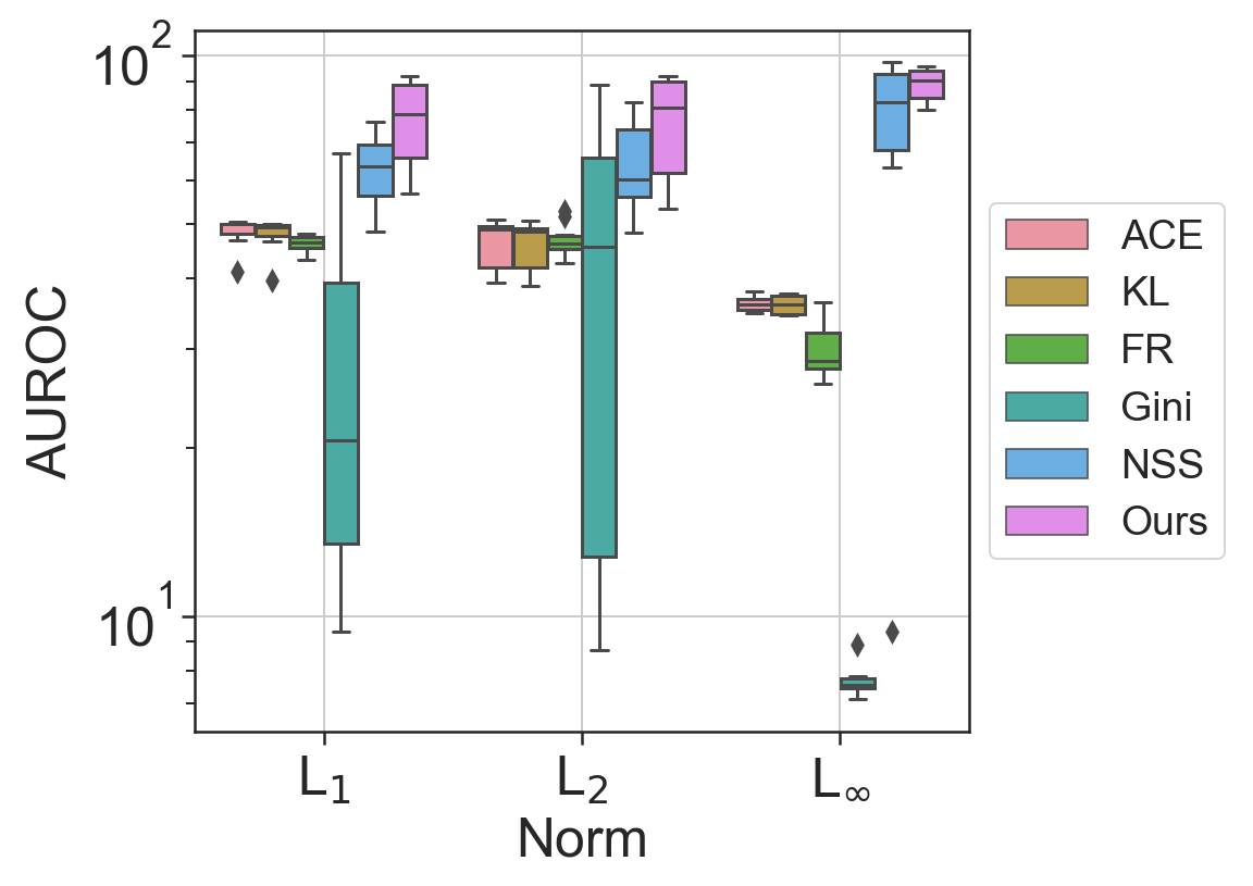
Figure 1: The shallow detectors are named after the loss function used to craft the attacks they are trained to detect. Overall, NSS clearly outperforms all the individual shallow detectors. The aggregation we propose allows us to use the shallow models to attain a detector whose performance is consistently comparable and in many cases better than NSS.

5.1 Evaluation Framework

Datasets and Pre-Trained Classifiers. We run our experiments on CIFAR10 [Krizhevsky, 2009] and SVHN [Netzer et al., 2011]. For both, the pre-trained target classifier is a ResNet-18 model that has been trained for $100$ epochs, using SGD optimizer with a learning rate of $0.1$, weight decay equal to $10^{-5}$, and momentum equal to $0.9$. The accuracy achieved by the classifiers on the original clean data is 99% for CIFAR10 and 100% for SVHN over the train split; 93.3% for CIFAR10 and 95.5% for SVHN over the test split.

Attack Strategies. We consider both white-box and, for completeness, black-box adversarial attacks For the white-box scenario, i.e. when the attacker has complete knowledge of the channel’s parameters, we consider Fast Gradient Sign Method (FGSM) [Goodfellow et al., 2015], Basic Iterative Method (BIM) [Kurakin et al.,] and Projected Gradient Descent (PGD) [Madry et al., 2018], Carlini-Wagner attack (CW) [Carlini and Wagner, 2017c] and DeepFool attack (DF) [Moosavi-Dezfooli et al., 2016]. In the case of black-box attacks, the adversary has no access to the internals of the target model, hence it creates attacks by querying the model and monitoring the outputs of the model to attack. Within this category of attacks we contemplate Square Attack (SA) [Andriushchenko et al., 2020], Hop Skip Jump attack (HOP) [Chen et al., 2020] and Spatial Transformation Attack (STA) [Engstrom et al., 2019]. We refer to the survey in [Aldahdooh et al., 2022] and references therein for an extensive discussion of this topic.

Mead [Granese et al., 2022]. The pre-trained classifier is attacked simultaneously with multiple attack strategies without extra information on the specific detector. To create a set of simultaneous attacks (cf. Tab. 1 in Sec. B.3), multiple perturbed versions of the same natural input sample are created according to the set of attack strategies, objective loss $\ell$, perturbation magnitude $\varepsilon$, and norm L_p. We consider $\ell$ to be either the Adversarial Cross Entropy loss (ACE) [Szegedy et al., 2014, Madry et al., 2018], or the Kullback-Leibler divergence (KL), or the Fisher-Rao objective (FR) [Picot et al., 2022] or the Gini Impurity score (Gini) [Granese et al., 2021]. The perturbed samples unable to fool the target classifier are discarded. Finally, the detector is evaluated on all the crafted adversarial examples, and only if all the attacks are correctly identified the detection is successful.

Detectors.

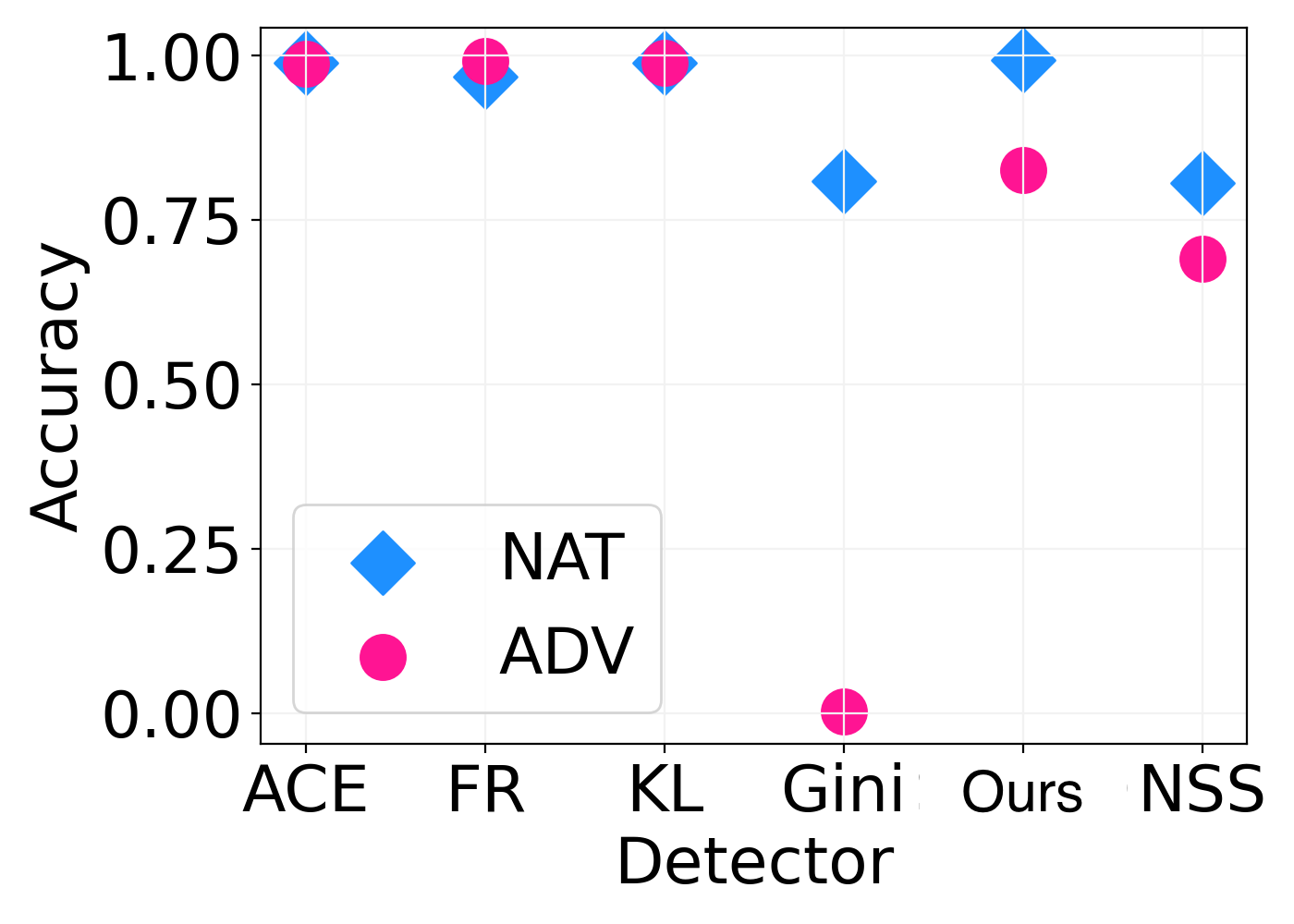
(a) Attacks with PGD algorithm, FR loss, $\varepsilon=40$, and norm L₁

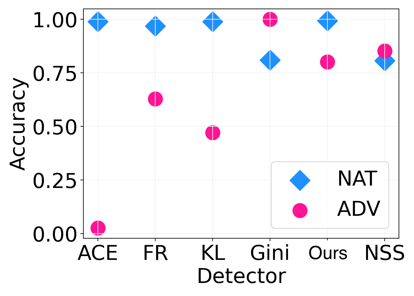
(b) Attacks with FGSM algorithm, FR loss, $\varepsilon=0.5$, and norm L_∞

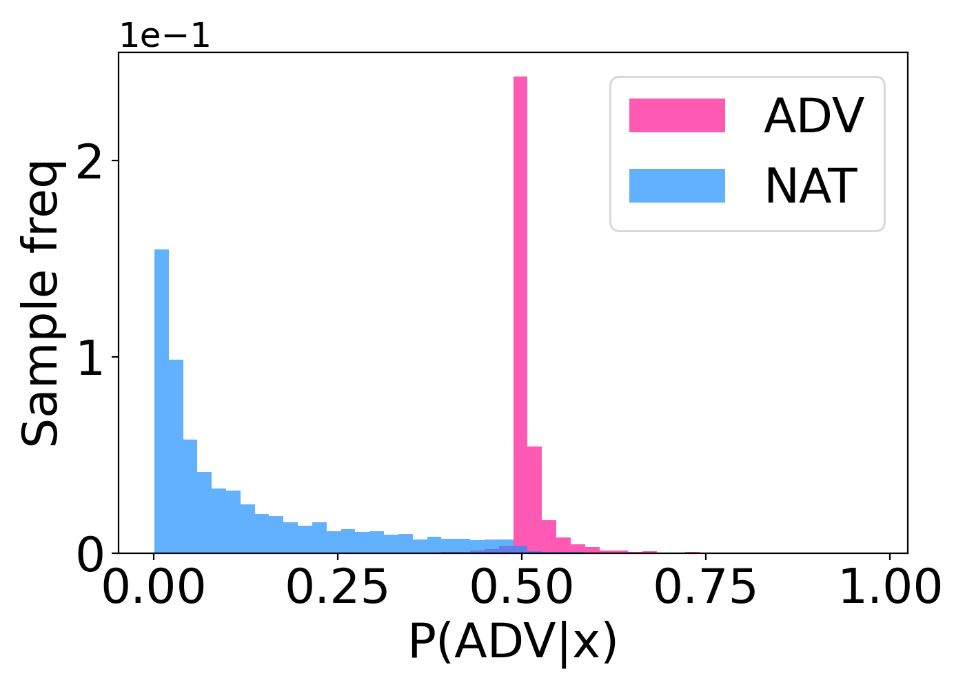
(c) Ours against attacks with PGD algorithm, FR loss, $\varepsilon=40$, and norm L₁

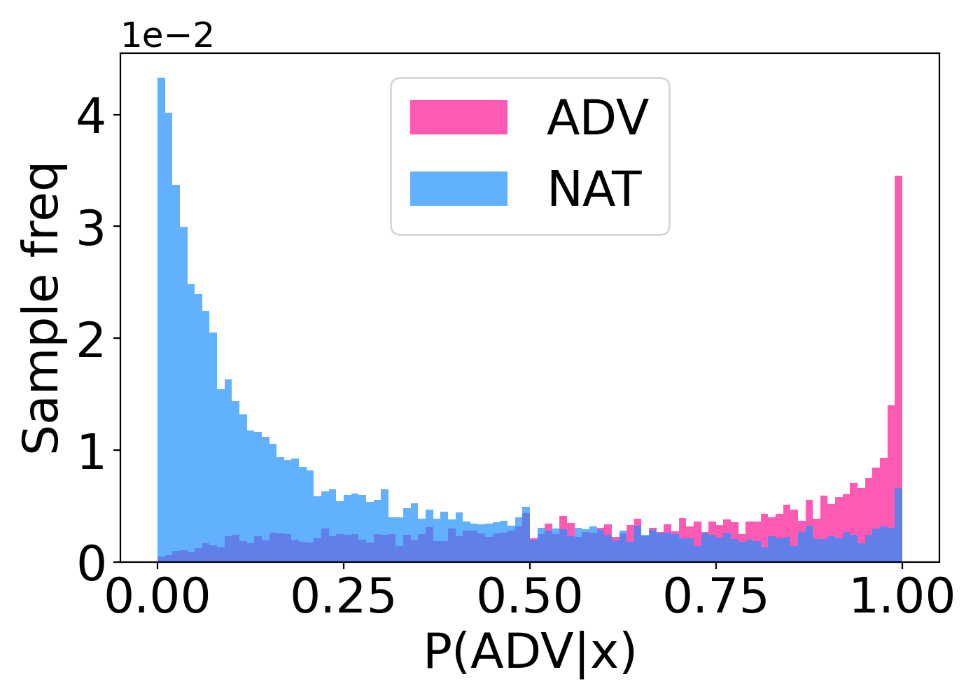
(d) NSS against attacks with PGD algorithm, FR loss, $\varepsilon=40$, and norm L₁

Figure 2: In Fig. 2(a) and Fig. 2(b), the accuracies of the detectors on natural and adversarial examples; in Fig. 2(c) and Fig. 2(d) we show how the proposed method and NSS split the data samples. We report the results for the detection of adversarial examples in pink, and the results for the detection of the natural in blue.

The proposed method aggregates four simple pre-trained detectors. The detectors are four fully-connected neural networks, composed of 3 layers of 256 nodes each. All the detectors are trained for 100 epochs, using SGD optimizer with learning rate of 0.01 and weight decay 0.0005. They are trained to distinguish between natural and adversarial examples created according to the PGD algorithm, under L_∞ norm constraint and perturbation magnitude $\varepsilon=0.125$ for CIFAR10 and $\varepsilon=0.25$ for SVHN. Each detector is trained on natural and adversarial examples generated using one of the loss functions mentioned in [Granese et al., 2022] (i.e., ACE Eq. (3), KL Eq. (4), FR Eq. (5), Gini Eq. (6) of the corresponding paper) to craft its adversarial training samples. We want to point out that the purpose of this paper is not to create a new supervised detector but rather to show a method to aggregate a set of pre-trained detectors. Moreover, it is important to notice that either supervised or unsupervised methods can be added to or pool of detectors, provided that their output is the confidence on the input sample being or not an adversarial example. We further expand on the selection of the $\varepsilon$ parameter of the adversarial examples used at training time in Sec. B.4 (cf. Tabs. 3 and 5).

NSS [Kherchouche et al., 2020]. We compare the proposed method with NSS, which is the best among the supervised SOTA methods against multi-armed adversarial attacks (cf. [Granese et al., 2022]). NSS characterizes the adversarial perturbations using natural scene statistics, i.e., statistical properties that the presence of adversarial perturbations can alter. NSS is trained by using PGD algorithm, L_∞ norm constraint and perturbation magnitude $\varepsilon=0.03125$ for CIFAR10 and $\varepsilon=0.0625$ for SVHN. We further expand on the selection of the $\varepsilon$ parameter of the adversarial examples used at training time in Tabs. 2, 4 and B.4.

Evaluation Metrics. For each sample and for each group of attacks we consider a detection successful, i.e. a true positive, if and only if all the adversarial attacks are detected. Otherwise, we report a false negative. We use the classical definitions of true negative and false positive for the natural samples detection. This means that a true negative is a natural sample detected as natural, and a false positive is a natural sample detected as adversarial. We measure the performance of the detectors in terms of $i)$ AUROC$\uparrow$% [Davis and Goadrich, 2006] (Area Under the Receiver Operating Characteristic curve), i.e., the detector’s ability to discriminate between adversarial and natural examples (higher is better); $ii)$ FPR at 95 % TPR (FPR$\downarrow_{95\%}$%), i.e., the percentage of natural examples detected as adversarial when 95 % of the adversarial are detected (lower is better).

5.2 Discussion

We present the main experimental results to show the effectiveness of the proposed method for multi-armed adversarial attack detection. Further discussion and additional results, can be found in Appendix B.

5.2.1 The Shallow Detectors

Figs. 2, 1 and 6 provides a graphical interpretation of the detection performance when the target classifier is ResNet18, trained on CIFAR10. The single detectors are named after the loss function used to craft the adversarial examples on which each detector is trained along with the natural samples. The main takeaway from Fig. 1 is the observation that, when considered individually, the shallow detectors are clearly subpar w.r.t. the SOTA adversarial attacks detection mechanism. On the contrary, the aggregation provided by our method results in detection performance that is comparable to SOTA performance and, in some cases, outperforms well-established detection mechanisms. Figure 6 sheds a light on the fact that the performance attained by our proposed method can consistently improve the detection of adversarial examples over several multi-armed attacks mounted using different norms and perturbation magnitudes.

A key insight of this paper is that when provided with generally non-robust detectors whose performance is good only against a limited amount of attacks (as it is confirmed by Figs. 1 and 6), we can successfully aggregate them through the proposed method to obtain a consistently better detection.

In Fig. 2 we consider attacks crafted according to the PGD algorithm, the FR loss, $\varepsilon=40$, and norm constraint L₁ (cf. Figs. 2(a), 2(c) and 2(d)), and attacks crafted according to the FGSM algorithm, FR loss, $\varepsilon=0.5$, and L_∞ norm in Fig. 2(b). We also report the performance of the considered detectors in terms of detection accuracy over the natural examples in blue and the adversarial examples in pink. As we can observe, the individual detectors, which are named after the loss functions ACE, FR, KL, and Gini, exhibit different behaviors for the specific attack. In Fig. 2(a), the Gini detector drastically fails at detecting the attack as its accuracy plummets to 0% on the adversarial examples. In the same way, the FR and KL detectors but mostly the ACE detector, perform poorly against FGSM (cf. Fig. 2(b)). On the contrary, our method, benefiting from the aggregation, obtains favorable results in both cases, confirming what we had observed.

The histograms in Figs. 2(c) and 2(d) show how the method we propose and NSS separate natural (blue) and adversarial examples (pink), respectively. The values along the horizontal axis represent the probability of being classified as adversarial, and the vertical axis represents the frequency of the samples within the bins. The detection error is proportional to the area of overlap between the blue and the pink histograms. Fig. 2(c) and Fig. 2(d) suggest that the proposed method achieves lower detection error on the considered attack, as it is confirmed in Tab. 18 where our proposed method attains 92.1 AUROC$\uparrow$%, while NSS only achieves 76.1 AUROC$\uparrow$%. Additional plots are provided in Sec. B.5.

5.2.2 Evaluation of the Proposed Solution in the Optimal Setting

(a) Attack loss: ACE

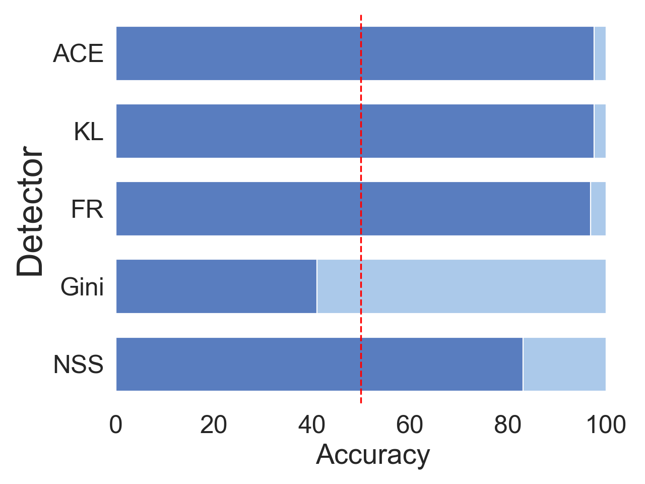
(b) Attack loss: KL

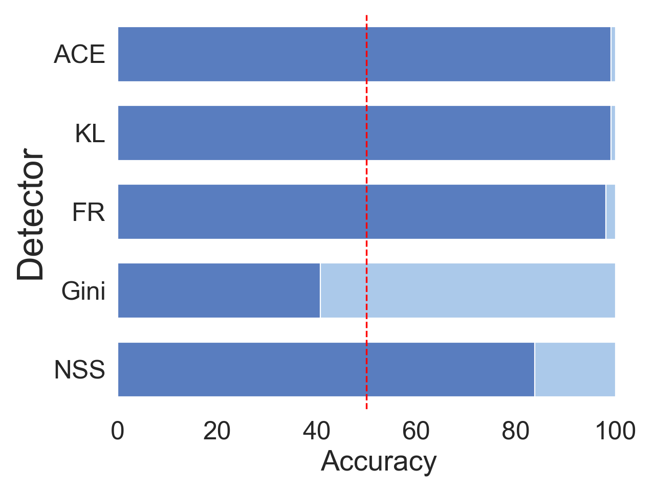
(c) Attack loss: FR

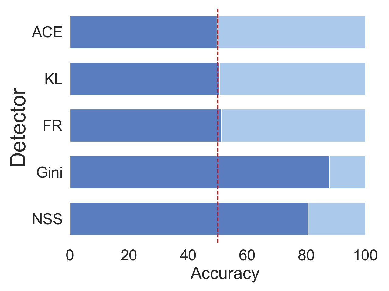
(d) Attack loss: Gini

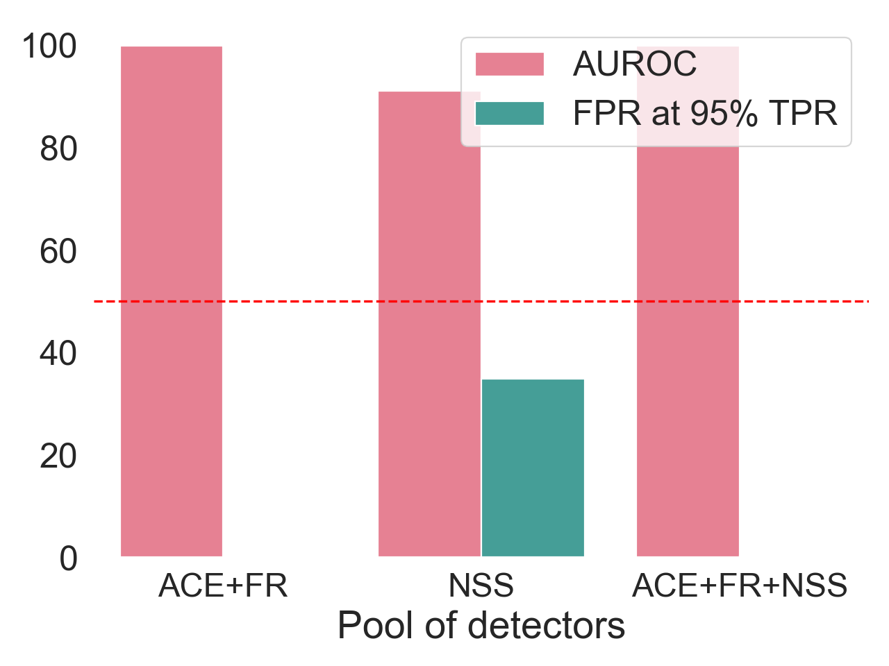
(e) Attack losses: ACE and FR

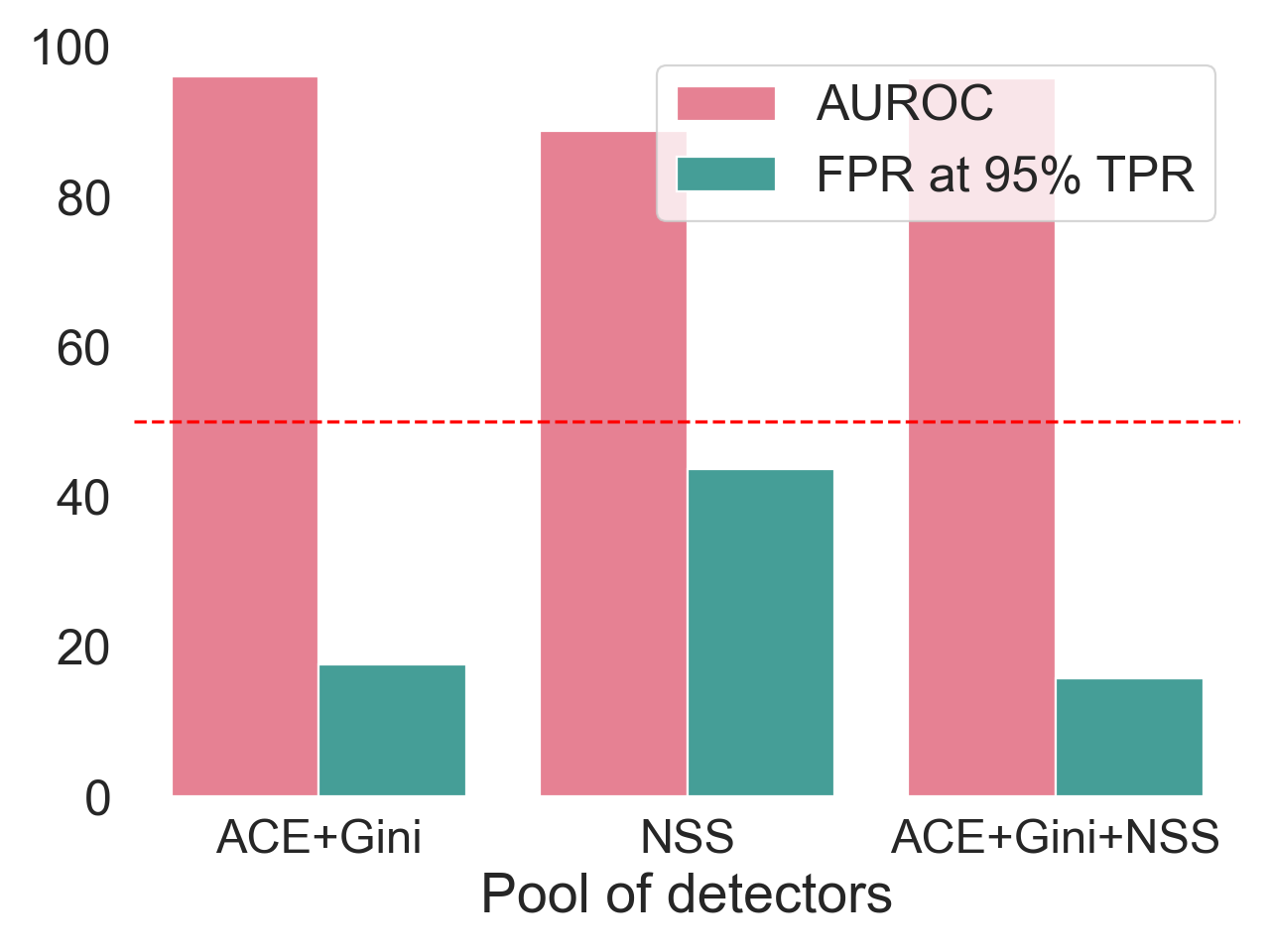
(f) Attack losses: ACE and Gini

(g) Attack losses: KL and Gini

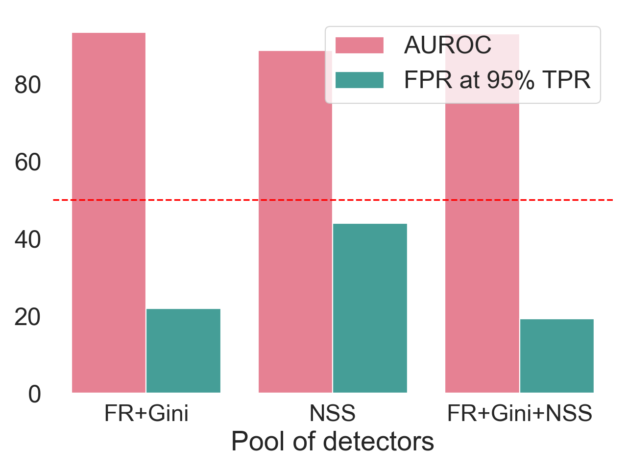
(h) Attack losses: FR and Gini

Figure 3: Attacks created with L_∞ norm, PGD and $\varepsilon=0.03125$. The attack losses are given in the captions. The shallow detectors are named after the loss function used to craft the attacks they are trained to detect.

In Fig. 3 we present an illustrative example on CIFAR10 of the aggregator behavior in the optimal setting, i.e., when there each detector in the considered set is trained to detect at least one strategy in the multi-arm scheme. This example considers attacks created using the PGD algorithm with L_∞ norm and $\varepsilon=0.03125$, and ACE loss in Fig. 3(a), KL loss in Fig. 3(b), FR loss in Fig. 3(c), and Gini loss in  Fig. 3(d). Note that, in the figures, the shallow detectors are named after the loss function used to craft the attacks they are trained to detect. As we operate within the optimal theoretical framework, in the figures when we mention the pool of detectors consisting of, for example, ACE+KL, it implies that multi-armed attacks are also created with ACE and KL losses. In Figs. 3(f), 3(g) and 3(h), even with just two detectors—one optimized for recognizing one specific type of attack and behaving poorly on the remaining one—we consistently observe an improvement in aggregator performance compared to the individual detector (i.e. NSS), which performs moderately well on both attacks. Moreover, in Fig. 3(e), we consider the setting in which all the detectors in the pool are able to detect each other attacks. Not surprisingly, the combination of the decisions brings positive results. These scenarios highlight the effectiveness of using a combination of specialized detectors, as opposed to relying on a single generalized detector for all attacks. Due to space limitations, the complete tables of results and those for SVHN, are in Sec. B.6.1.

5.2.3 Evaluation of the Proposed Solution in the Setting of [Granese et al., 2022]

We continue our evaluation by considering the Mead setup in [Granese et al., 2022] where the assumptions of the optimal setting are not met. The numerical results are provided in Appendix B (Tab. 18) for space reasons. On CIFAR10, our aggregator achieves the maximum AUROC improvement of 79.5 percentage points compared to NSS. This improvement occurs for attacks under $L_{\infty}$-norm constraint, $\varepsilon=0.125$ and PGD^⋆, FGSM^⋆, BIM^⋆, SA, i.e. when as many as 13 different simultaneous adversarial attacks are mounted. Similarly, for our proposed method the maximum attained FPR at 95% TPR improvement w.r.t. NSS is 90.3 percentage points and happens for attacks under $L_{\infty}$-norm constraint, $\varepsilon=0.5$ and PGD^⋆, FGSM^⋆, BIM^⋆, i.e. when as many as 12 different simultaneous adversarial attacks are mounted. Our aggregator outperforms NSS in the case of the attacks with L₁ and L₂ norm, regardless of the algorithm or the perturbation magnitude, and in the case of L_∞ norm with large perturbations. However, for the attacks with L_∞ norm and small $\varepsilon$, although the proposed method’s performance is comparable to that of NSS, we notice a slight degradation. To shed light on this, we remind that individual detectors aggregated are based on the classifier’s logits; NSS, on the other hand, extracts natural scene statistics from the inputs. This more sophisticated technique makes NSS perform well when tested on attacks with similar $\varepsilon$ and the same norm as the ones seen at training time. Additionally, it is essential to emphasize that the evaluation setting considered in the following analysis introduces additional challenges compared to the theoretical framework. In this evaluation, there may be cases where none of the detectors are optimal for the attacks under consideration. While this adds complexity, it reflects common real-life scenarios. Similar conclusions can be drawn for the results on SVHN (cf. Tab. 18). In Sec. B.7.1 we conduct an in-depth analysis of the ablation study for this specific evaluation setup.

6 CONCLUDING REMARKS

We introduce a zero-shot method to detect attacks mounted against a target channel by a multi-armed malicious actor that can alter the input signal in an adversarial way. We characterized our theoretically optimal soft-detector which aggregates the decision of detection mechanisms, whose individual performance are poor in the multi-armed attack scenario, as the solution to a minimax problem where the defense minimizes the maximum risk due to the multi-armed attacker. Our empirical results, tailored to the domain of adversarial example detection, show that aggregating simple detectors using our method results in consistently improved detection performance. The achieved performance is comparable and in a large set of cases better than the best state-of-the-art (SOTA) method in the multi-armed attack scenarios. Our method has two key benefits: it is modular, allowing existing and future methods to be integrated (whether they are supervised or unsupervised), and it is general, able to recognize adversarial examples from various attack algorithms and loss functions. In general, adaptive attacks mounted on individual detectors are an argument in favor of other approaches to the problem (cf. Sec. B.9). We argue that, in our framework, we can rely on the effect redundancy to make sure that the task of mounting adaptive attacks on multiple detectors, possibly effective against the same attack strategy, becomes expensive or, at least, prohibitively expensive for an attacker. We leave the exploration of this aspect to future work. Finally, our work to be applicable to other problems, such as intrusion, anomaly, out-of-distribution, or backdoor detection.

Acknowledgments

The work of Federica Granese was supported by the ANR-20-CE17-0022 DeepECG4U funding from the French National Research Agency.

Checklist

1. For all models and algorithms presented, check if you include:

   1. A clear description of the mathematical setting, assumptions, algorithm, and/or model. Yes (Secs. 2 and 3)

   2. An analysis of the properties and complexity (time, space, sample size) of any algorithm. Yes (Sec. B.1)

   3. (Optional) Anonymized source code, with specification of all dependencies, including external libraries. Yes (Supplementary materials)

2. For any theoretical claim, check if you include:

   1. Statements of the full set of assumptions of all theoretical results. Yes (Secs. 2 and 3)

   2. Complete proofs of all theoretical results. Yes (Sec. A.1)

   3. Clear explanations of any assumptions. Yes (Secs. 2 and 3)

3. For all figures and tables that present empirical results, check if you include:

   1. The code, data, and instructions needed to reproduce the main experimental results (either in the supplemental material or as a URL). Code available at https://github.com/fgranese/Optimal-Zero-Shot-Detector-for-Multi-Armed-Attacks.

   2. All the training details (e.g., data splits, hyperparameters, how they were chosen). Yes (Secs. 5.1 and B)

   3. A clear definition of the specific measure or statistics and error bars (e.g., with respect to the random seed after running experiments multiple times). Not Applicable

   4. A description of the computing infrastructure used. (e.g., type of GPUs, internal cluster, or cloud provider). Yes (Sec. B.1)

4. If you are using existing assets (e.g., code, data, models) or curating/releasing new assets, check if you include:

   1. Citations of the creator If your work uses existing assets. Yes (for CIFAR10 and SVHN datasets, Sec. 5.1)

   2. The license information of the assets, if applicable. Not Applicable (Open source)

   3. New assets either in the supplemental material or as a URL, if applicable. Not Applicable

   4. Information about consent from data providers/curators. Not Applicable

   5. Discussion of sensible content if applicable, e.g., personally identifiable information or offensive content. Not Applicable

5. If you used crowdsourcing or conducted research with human subjects, check if you include:

   1. The full text of instructions given to participants and screenshots. Not Applicable

   2. Descriptions of potential participant risks, with links to Institutional Review Board (IRB) approvals if applicable. Not Applicable

   3. The estimated hourly wage paid to participants and the total amount spent on participant compensation. Not Applicable

 

Supplementary Materials

 

Appendix A SUPPLEMENTARY DETAILS ON SEC. 3

A.1 Proofs

A.1.1 Proof of Eq. 3

Proof.

$$\max_{k\in\mathcal{K}}\,\mathbb{E}_{q^{(k)}_{\widehat{Z}|\mathbf{u_{0}}}}\left[-\log{q}_{\widehat{Z}|\mathbf{u_{0}}}\right] =\max_{k\in\mathcal{K}}\,\left[\mathbb{E}_{q^{(k)}_{\widehat{Z}|\mathbf{u_{0}}}}\left[-\log q^{(k)}_{\widehat{Z}|\mathbf{u_{0}}}\right]+\mathbb{E}_{q^{(k)}_{\widehat{Z}|\mathbf{u_{0}}}}\left[\log\left(\frac{q^{(k)}_{\widehat{Z}|\mathbf{u_{0}}}}{{q}_{\widehat{Z}|\mathbf{u_{0}}}}\right)\right]\right]$$

$$\leq\max_{k\in\mathcal{K}}\,\mathbb{E}_{q^{(k)}_{\widehat{Z}|\mathbf{u_{0}}}}\left[-\log q^{(k)}_{\widehat{Z}|\mathbf{u_{0}}}\right]+\max_{k\in\mathcal{K}}\,\mathbb{E}_{q^{(k)}_{\widehat{Z}|\mathbf{u_{0}}}}\left[\log\left(\frac{q^{(k)}_{\widehat{Z}|\mathbf{u_{0}}}}{{q}_{\widehat{Z}|\mathbf{u_{0}}}}\right)\right].$$

∎

A.1.2 Proof of Sec. 3

Proof.

The equality holds by noticing that

$$\max_{P_{\Omega}} \,\mathbb{E}_{\Omega}\left[D_{\textrm{KL}}\left(q^{(\Omega)}_{\widehat{Z}|\mathbf{u_{0}}}\big{\|}{q}_{\widehat{Z}|\mathbf{u_{0}}}\right)\right]\leq\max_{k\in\mathcal{K}}\,\mathbb{E}_{q^{(k)}_{\widehat{Z}|\mathbf{u_{0}}}}\left[\log\left(\frac{q^{(k)}_{\widehat{Z}|\mathbf{u_{0}}}}{{q}_{\widehat{Z}|\mathbf{u_{0}}}}\right)\right],$$

and moreover,

$$\max_{k\in\mathcal{K}}\,\mathbb{E}_{q^{(k)}_{\widehat{Z}|\mathbf{u_{0}}}}\left[\log\left(\frac{q^{(k)}_{\widehat{Z}|\mathbf{u_{0}}}}{{q}_{\widehat{Z}|\mathbf{u_{0}}}}\right)\right] =\mathbb{E}_{\bar{\Omega}}\left[D_{\textrm{KL}}\left(q^{(\bar{\Omega})}_{\widehat{Z}|\mathbf{u_{0}}}\big{\|}{q}_{\widehat{Z}|\mathbf{u_{0}}}\right)\right],$$

by choosing the random variable $\bar{\Omega}$ with uniform probability over the set of maximizers ${\overline{\mathcal{K}}=\arg\max_{k\in\mathcal{K}}\,\mathbb{E}_{q^{(k)}_{\widehat{Z}|\mathbf{u_{0}}}}\left[\log\left(\frac{q^{(k)}_{\widehat{Z}|\mathbf{u_{0}}}}{{q}_{\widehat{Z}|\mathbf{u_{0}}}}\right)\right]}$, zero otherwise. ∎

A.1.3 Proof of Sec. 3

Proof.

We consider a zero-sum game with a concave-convex mapping defined on a product of convex sets. The sets of all probability distributions ${q}_{\widehat{Z}|\mathbf{u_{0}}}$ and $P_{\Omega}$ are two nonempty convex sets, bounded and finite-dimensional. On the other hand, $\big{(}P_{\Omega},{q}_{\widehat{Z}|\mathbf{u_{0}}}\big{)}\rightarrow\mathbb{E}_{\Omega}\left[D_{\textrm{KL}}\left(q^{(\Omega)}_{\widehat{Z}|\mathbf{u_{0}}}\big{\|}{q}_{\widehat{Z}|\mathbf{u_{0}}}\right)\right]$ is a concave-convex mapping, i.e., $P_{\Omega}\rightarrow\mathbb{E}_{\Omega}\left[D_{\textrm{KL}}\left(q^{(\Omega)}_{\widehat{Z}|\mathbf{u_{0}}}\big{\|}{q}_{\widehat{Z}|\mathbf{u_{0}}}\right)\right]$ is concave and ${q}_{\widehat{Z}|\mathbf{u_{0}}}\rightarrow\mathbb{E}_{\Omega}\left[D_{\textrm{KL}}\left(q^{(\Omega)}_{\widehat{Z}|\mathbf{u_{0}}}\big{\|}{q}_{\widehat{Z}|\mathbf{u_{0}}}\right)\right]$ is convex for every $\big{(}P_{\Omega},{q}_{\widehat{Z}|\mathbf{u_{0}}}\big{)}$. Then, by classical min-max theorem  [von Neumann, 1928] we have that Sec. 3 holds. ∎

A.1.4 Proof of Eq. 6

Proof.

It is enough to show that

$$\min_{\widehat{q}_{\widehat{Z}|\mathbf{u_{0}}}}\mathbb{E}_{\Omega}\left[D_{\textrm{KL}}\left(q^{(\Omega)}_{\widehat{Z}|\mathbf{u_{0}}}\big{\|}{q}_{\widehat{Z}|\mathbf{u_{0}}}\right)\right]=I_{\mathbf{u_{0}}}(\Omega;\widehat{Z}),$$ (12)

for every random variable $\Omega$ distributed according to an arbitrary probability distribution $P_{\Omega}$ and each distribution $q^{(\Omega)}_{\widehat{Z}|\mathbf{u_{0}}}$. We begin by showing that

$$\mathbb{E}_{\Omega}\left[D_{\textrm{KL}}\left(q^{(\Omega)}_{\widehat{Z}|\mathbf{u_{0}}}\big{\|}{q}_{\widehat{Z}|\mathbf{u_{0}}}\right)\right] \geq I_{\mathbf{u_{0}}}(\Omega;\widehat{Z}),$$

for any arbitrary distributions $P_{\Omega}$ and $q^{(\Omega)}_{\widehat{Z}|\mathbf{u_{0}}}$. To this end, we use the following identities:

$$\mathbb{E}_{\Omega}\left[D_{\textrm{KL}}\left(q^{(\Omega)}_{\widehat{Z}|\mathbf{u_{0}}}\big{\|}{q}_{\widehat{Z}|\mathbf{u_{0}}}\right)\right] =\mathbb{E}_{\Omega}\mathbb{E}_{q^{(\Omega)}_{\widehat{Z}|\mathbf{u_{0}}}}\left(\log\frac{q^{(\Omega)}_{\widehat{Z}|\mathbf{u_{0}}}}{{q}_{\widehat{Z}|\mathbf{u_{0}}}}\right)$$

$$=\mathbb{E}_{\Omega}\mathbb{E}_{q^{(\Omega)}_{\widehat{Z}|\mathbf{u_{0}}}}\left(\log\frac{q^{(\Omega)}_{\widehat{Z}|\mathbf{u_{0}}}}{P_{\widehat{Z}}}\right)+D_{\textrm{KL}}\left(P_{\widehat{Z}}\|{q}_{\widehat{Z}|\mathbf{u_{0}}}\right)$$

$$=I_{\mathbf{u_{0}}}(\Omega;\widehat{Z})+D_{\textrm{KL}}\left(P_{\widehat{Z}}\|{q}_{\widehat{Z}|\mathbf{u_{0}}}\right)\geq I_{\mathbf{u_{0}}}(\Omega;\widehat{Z}),$$ (13)

where $P_{\widehat{Z}}$ denotes the marginal distribution of $q^{(\Omega)}_{\widehat{Z}|\mathbf{u_{0}}}$ w.r.t. $P_{\Omega}$ and the last inequality follows since the KL divergence is positive. Finally, it is easy to check that by selecting ${q}_{\widehat{Z}|\mathbf{u_{0}}}=P_{\widehat{Z}}$ the lower bound in (13) is achieved which proves the identity in expression (12). By taking the maximum overall probability distributions $P_{\Omega}$ at both sides of expression (12) the claim follows. ∎

A.1.5 Proof of the Result in Sec. 3.1

This proof is adapted from [Ben-David et al., 2010].

Proof.

$$P_{e}^{T}(\textsc{D}) =P_{e}^{T}(\textsc{D})+P_{e}^{S}(\textsc{D})-P_{e}^{S}(\textsc{D})+\mathbb{E}_{\mathbf{x}\sim P^{S}_{X}}\left[\mathds{1}\left[\textsc{D}\left(\mathbf{x}\right)\neq f^{T}(\mathbf{x})\right]\right]-\mathbb{E}_{\mathbf{x}\sim P^{S}_{X}}\left[\mathds{1}\left[\textsc{D}\left(\mathbf{x}\right)\neq f^{T}(\mathbf{x})\right]\right]$$ (14)

$$\leq P_{e}^{S}(\textsc{D})+\left|\mathbb{E}_{\mathbf{x}\sim P^{S}_{X}}\left[\mathds{1}\left[\textsc{D}\left(\mathbf{x}\right)\neq f^{T}(\mathbf{x})\right]\right]-P_{e}^{S}(\textsc{D})\right|+\left|P_{e}^{T}(\textsc{D})-\mathbb{E}_{\mathbf{x}\sim P^{S}_{X}}\left[\mathds{1}\left[\textsc{D}\left(\mathbf{x}\right)\neq f^{T}(\mathbf{x})\right]\right]\right|$$ (15)

$$\leq P_{e}^{S}(\textsc{D})+\mathbb{E}_{\mathbf{x}\sim P^{S}_{X}}\left|\mathds{1}\left[\textsc{D}\left(\mathbf{x}\right)\neq f^{T}(\mathbf{x})\right]-\mathds{1}\left[\textsc{D}\left(\mathbf{x}\right)\neq f^{S}(\mathbf{x})\right]\right|+\left|P_{e}^{T}(\textsc{D})-\mathbb{E}_{\mathbf{x}\sim P^{S}_{X}}\left[\mathds{1}\left[\textsc{D}\left(\mathbf{x}\right)\neq f^{T}(\mathbf{x})\right]\right]\right|$$ (16)

$$\leq P_{e}^{S}(\textsc{D})+\mathbb{E}_{\mathbf{x}\sim P^{S}_{X}}\left|f^{T}(\mathbf{x})-f^{S}(\mathbf{x})\right|+\left|P_{e}^{T}(\textsc{D})-\mathbb{E}_{\mathbf{x}\sim P^{S}_{X}}\left[\mathds{1}\left[\textsc{D}\left(\mathbf{x}\right)\neq f^{T}(\mathbf{x})\right]\right]\right|$$ (17)

$$\leq P_{e}^{S}(\textsc{D})+\mathbb{E}_{\mathbf{x}\sim P^{S}_{X}}\left|f^{T}(\mathbf{x})-f^{S}(\mathbf{x})\right|+d\left(P^{S}_{X|Z=1},P^{T}_{X|Z=1}\right).$$ (18)

Notice that by choosing to add and subtract $\mathbb{E}_{\mathbf{x}\sim P^{T}_{X}}\left[\mathds{1}\left[\textsc{D}\left(\mathbf{x}\right)\neq f^{T}(\mathbf{x})\right]\right]$ instead of $\mathbb{E}_{\mathbf{x}\sim P^{S}_{X}}\left[\mathds{1}\left[\textsc{D}\left(\mathbf{x}\right)\neq f^{T}(\mathbf{x})\right]\right]$, we would get the term $\mathbb{E}_{\mathbf{x}\sim P^{T}_{X}}\left|f^{T}(\mathbf{x})-f^{S}(\mathbf{x})\right|$, instead of $\mathbb{E}_{\mathbf{x}\sim P^{S}_{X}}\left|f^{T}(\mathbf{x})-f^{S}(\mathbf{x})\right|$. Therefore, the final result holds true:

$$P_{e}^{T}(\textsc{D}) \leq P_{e}^{S}(\textsc{D})+d\left(P^{S}_{X|Z=1},P^{T}_{X|Z=1}\right)$$

$$+\min\big{\{}\mathbb{E}_{\mathbf{x}\sim P^{S}_{X}}[|f^{S}(\mathbf{x})-f^{T}(\mathbf{x})|],$$

$$\mathbb{E}_{\mathbf{x}\sim P^{T}_{X}}[|f^{S}(\mathbf{x})-f^{T}(\mathbf{x})|]\big{\}}.$$ (19)

∎

A.2 On the Optimization of Eq. 6

The maximization problem in Eq. 6 is well-posed given that the mutual information is a concave function of $\omega\in\Omega$. Although from the theoretical point of view, Eq. 6 guarantees the optimal solution for the average regret minimization problem, in practice, we have to deal with some technical limitations.

For the optimization of  Eq. 6, we rely on the implementation of the Blahut-Arimoto algorithm [Arimoto, 1972]. This is an iterative algorithm for finding the capacity, $C$, of a channel that in our context corresponds to objective in Eq. 6 i.e., $C=\underset{w_{k}}{\max}\,I_{\mathbf{u}_{0}}(\Omega;\widehat{Z})$. Therefore, at iteration $t+1$ the weights $\omega^{t+1}_{k}$ to associate with the decision made by the detector $k$ will be computed as follows

$$\tilde{\omega}^{t+1}_{k}(z) =\frac{\omega^{t}_{k}\cdot(q^{(k)}_{\widehat{Z}=z|\mathbf{u}_{0}})}{\sum_{k=0}^{K}\,\omega^{t}_{k}\cdot(q^{(k)}_{\widehat{Z}=z|\mathbf{u}_{0}})}$$ (20)

$$\omega^{t+1}_{k} =\frac{\prod_{z\in\{0,1\}}\tilde{\omega}^{t+1}_{k}(z)^{(q^{(k)}_{\widehat{Z}=z|\mathbf{u}_{0}})}}{\sum_{k=0}^{K}\prod_{z\in\{0,1\}}\tilde{\omega}^{t+1}_{k}(z)^{(q^{(k)}_{\widehat{Z}=z|\mathbf{u}_{0}})}},$$ (21)

where $K$ denotes the number of detectors to aggregate. Overall, we obtained the satisfactory results provided in the paper by assigning default values to all the parameters and by setting a uniform distribution $[\omega_{1},\omega_{2},\omega_{3},\omega_{4}]=[.25,.25,.25,.25]$ as the initial point in the solutions space.

Appendix B ADDITIONAL EXPERIMENTS

B.1 Experimental Environment and Time Measurements

We run each experiment on a machine equipped with an Intel(R) Xeon(R) Gold 6226 CPU, 2.70GHz clock frequency, and a Tesla V100-SXM2-32GB GPU.

Training 1 single detector in our method	1h45m10s
Evaluating the optimization in our method	5s (for one attack)
Training NSS	3m30s
Evaluating NSS	20s (for one attack)
On the largest set of simultaneous attacks (13 attacks):
Ours	5s * 13 $\sim$ 65s
NSS	20s * 13 $\sim$ 4m

B.2 State-of-the-Art (SOTA) Detectors

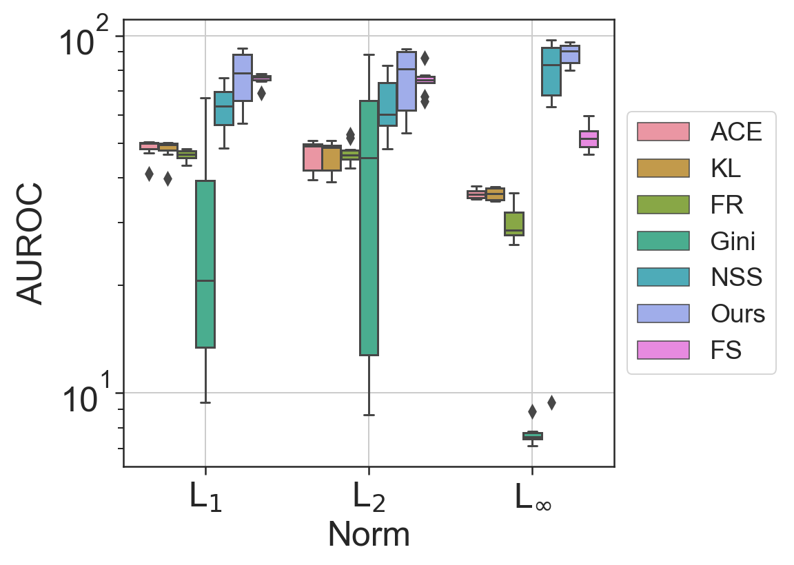
Figure 4: The shallow detectors are named after the loss function used to craft the attacks they are trained to detect.

[Granese et al., 2022] suggests NSS [Kherchouche et al., 2020] and FS [Xu et al., 2018] as the most robust methods in the simultaneous attacks detection scheme (i.e., Mead). We remind that NSS is a supervised method that extracts the natural scene statistics of the natural and adversarial examples to train a SVM. On the contrary, FS is an unsupervised method that uses feature squeezing (i.e., reducing the color depth of images and using smoothing to reduce the variation among the pixels) to compare the model’s predictions.

In particular, we choose NSS as a method to compare for multiple reasons:

1. NSS achieves the best overall score in terms of AUROC$\uparrow$% and FPR$\downarrow_{95\%}$% among the SOTA against simultaneous attacks (cf. Tab. 3 [Granese et al., 2022]).

2. NSS achieves the best score in terms of AUROC$\uparrow$% and FPR$\downarrow_{95\%}$% under the L_∞ norm where the biggest group of simultaneous attacks are evaluated (see Tab. 1). This is stressed in the plots in Fig. 4. Moreover, FS reaches better performance w.r.t. the proposed method only with PGD1 and PGD2 when the perturbation magnitude is small and in CW2.

3. The case study for our aggregator in the experimental section is based on supervised detectors as a consequence the comparison with a supervised detector was a natural choice.

For the sake of completeness, the performances of NSS and FS under Mead are given in Fig. 4.

B.3 Attacks

Table 1: Each cell corresponds to attacks simultaneously executed on the targeted classifier. Attacks created using all the losses in [Granese et al., 2022] are marked with ^⋆. Attacks such as SA and DF are not dependent on the choice for the loss, but are equally considered as part of the multi-armed framework. Empty cells correspond to combinations of perturbation magnitude and norm constraint that are usually not considered in the literature.

	L1	L2	L∞	No norm
$\varepsilon=0.01$	-	CW2	-	-
$\varepsilon=0.03125$	-	-	PGDi⋆,FGSM⋆,BIM⋆	-
$\varepsilon=0.0625$	-	-	PGDi⋆,FGSM⋆,BIM⋆	-
$\varepsilon=0.1$	-	HOP	-	-
$\varepsilon=0.125$	-	PGD2⋆	PGDi⋆,FGSM⋆,BIM⋆,SA	-
$\varepsilon=0.25$	-	PGD2⋆	PGDi⋆,FGSM⋆,BIM⋆	-
$\varepsilon=0.3125$	-	PGD2⋆	PGDi⋆,FGSM⋆,BIM⋆,CWi	-
$\varepsilon=0.5$	-	PGD2⋆	PGDi⋆,FGSM⋆,BIM⋆	-
$\varepsilon=1$	-	PGD2⋆	-	-
$\varepsilon=1.5$	-	PGD2⋆	-	-
$\varepsilon=2$	-	PGD2⋆	-	-
$\varepsilon=5$	PGD1⋆	-	-	-
$\varepsilon=10$	PGD1⋆	-	-	-
$\varepsilon=15$	PGD1⋆	-	-	-
$\varepsilon=20$	PGD1⋆	-	-	-
$\varepsilon=25$	PGD1⋆	-	-	-
$\varepsilon=30$	PGD1⋆	-	-	-
$\varepsilon=40$	PGD1⋆	-	-	-
No $\varepsilon$	-	DF	-	-
max. rotation $=30$ max. translation $=8$	-	-	-	STA

We want to emphasize that, differently from the literature, we are the first to consider a defense mechanism against the simultaneous attack setting in which we detect attacks based on four different losses. More specifically, for each ’clean dataset’ (in our case CIFAR10 and SVHN):

• No. of adversarial examples generated with:

  • L₁ norm: 7 (no. of $\varepsilon$) * 1 (PGD algorithm) * 4 (no. of losses) = 28 (’adversarial datasets’)

  • L₂ norm: 7 (no. of $\varepsilon$) * 1 (PGD algorithm) * 4 (no. of losses) + 3 (CW2, HOP, DeepFool) = 31 (’adversarial datasets’)

  • L_∞ norm: 6 (no. of $\varepsilon$) * 3 (PGD, FGSM, BIM algorithms) * 4 (no. of losses) + 2 = 74 (’adversarial datasets’)

  • No norm: 1 (’adversarial dataset’)

• For a total of 28 + 31 + 74 + 1 = 134 ’adversarial datasets’ for each ’clean dataset’.

Moreover, it is interesting to notice that the experiments on CIFAR10 and SVHN represent a satisfying choice to show that state-of-the-art detection mechanisms struggle to maintain good performance when they are faced with the framework of simultaneous attacks. That said, we leave the evaluation of larger datasets as future work.

We provide in Tab. 1 below how the attacks are grouped in the evaluation of the multi-armed setting

B.4 Simulations Adversarial Attack According to Different $\varepsilon$

As discussed in Sec. 5.1, both NSS and the shallow detectors aggregated via the proposed method are trained on natural and adversarial examples created with PGD algorithm and L_∞ norm constraint. We show in Tabs. 2, 3, 4 and 5 the results of the two methods according to $\varepsilon\in\left\{.03125,.0625,.125,.25,.3125,.5\right\}$.

Table 2: Simultaneous attacks detection: NSS on CIFAR10. We train NSS on natural and adversarial examples created with PGD algorithm and L_∞ norm constraint. The perturbation magnitude $\varepsilon$ is shown in the columns. We indicate in bold the best result.

	NSS
	0.03125		0.0625		0.125		0.25		0.3125		0.5
	AUROC$\uparrow$%	FPR$\downarrow_{95\%}$%	AUROC$\uparrow$%	FPR$\downarrow_{95\%}$%	AUROC$\uparrow$%	FPR$\downarrow_{95\%}$%	AUROC$\uparrow$%	FPR$\downarrow_{95\%}$%	AUROC$\uparrow$%	FPR$\downarrow_{95\%}$%	AUROC$\uparrow$%	FPR$\downarrow_{95\%}$%
Norm L1
PGD1
$\varepsilon$ = 5	48.5	94.2	47.7	94.7	46.6	95.6	46.8	95.5	47.0	95.4	46.5	95.6
$\varepsilon$ = 10	54.0	90.3	53.4	90.8	51.6	94.3	50.4	94.9	50.4	94.9	50.9	94.7
$\varepsilon$ = 15	58.8	86.8	58.1	87.4	55.8	92.8	53.8	94.2	53.2	94.4	54.5	93.7
$\varepsilon$ = 20	63.5	82.3	62.7	82.7	60.1	90.7	57.4	93.2	56.7	93.6	58.2	92.3
$\varepsilon$ = 25	67.7	77.2	66.8	78.4	64.0	87.8	61.0	92.0	60.1	92.6	61.9	90.6
$\varepsilon$ = 30	71.4	73.4	70.5	73.5	67.6	83.7	64.4	90.4	63.4	91.4	65.4	88.2
$\varepsilon$ = 40	76.1	67.3	75.3	68.0	72.6	75.4	69.4	87.2	68.5	88.9	70.4	83.4
Norm L2
PGD2
$\varepsilon$ = 0.125	48.3	94.3	47.5	94.8	46.6	95.6	46.7	95.5	47.1	95.4	46.5	95.6
$\varepsilon$ = 0.25	53.2	91.2	52.6	91.6	50.9	94.6	50.0	95.0	50.0	95.0	50.3	94.8
$\varepsilon$ = 0.3125	55.8	89.2	55.2	89.9	53.3	93.7	51.7	94.6	51.5	94.7	52.3	94.3
$\varepsilon$ = 0.5	63.3	82.6	62.6	83.0	60.0	90.7	57.4	93.2	56.7	93.5	58.2	92.4
$\varepsilon$ = 1	76.4	67.5	75.7	67.8	73.1	75.0	70.1	86.7	69.2	88.5	71.0	83.0
$\varepsilon$ = 1.5	81.0	63.0	80.5	62.7	78.5	63.5	76.2	80.7	75.6	83.2	76.9	74.4
$\varepsilon$ = 2	82.6	62.3	82.1	61.6	80.6	62.5	78.6	78.5	78.1	81.2	79.1	72.1
DeepFool
No $\varepsilon$	57.0	91.7	56.7	91.7	55.6	93.6	54.6	94.1	54.2	94.3	54.7	94.0
CW2
$\varepsilon$ = 0.01	56.4	90.8	55.9	90.9	54.5	93.7	53.4	94.3	53.0	94.5	53.6	94.1
HOP
$\varepsilon$ = 0.1	66.1	87.0	65.1	88.2	63.0	91.3	61.2	92.6	60.8	92.9	61.6	92.1
Norm L∞
PGDi, FGSM, BIM
$\varepsilon$ = 0.03125	83.0	55.3	82.1	55.2	80.3	57.8	77.4	77.0	76.8	81.3	78.3	65.4
$\varepsilon$ = 0.0625	96.0	17.2	94.6	17.4	94.9	19.2	94.3	21.6	94.4	21.1	94.4	21.1
$\varepsilon$ = 0.25	97.3	0.6	94.7	5.9	96.5	2.5	96.9	1.7	97.2	1.1	96.7	2.1
$\varepsilon$ = 0.5	82.5	100.0	80.4	100.0	81.9	100.0	82.2	100.0	82.4	100.0	82.0	100.0
PGDi, FGSM, BIM, SA
$\varepsilon$ = 0.125	9.4	99.9	10.4	100.0	26.2	99.9	30.9	100.0	33.8	100.0	27.3	100.0
PGDi, FGSM, BIM, CWi
$\varepsilon$ = 0.3125	63.2	99.1	62.7	99.0	61.9	99.3	60.9	99.5	60.5	99.5	61.2	99.4
No norm
STA
No $\varepsilon$	88.5	38.8	92.0	25.1	92.1	22.4	93.3	18.3	92.7	19.6	92.7	19.7

Table 3: Simultaneous attacks detection: the proposed method on CIFAR10. We train the detectors on natural and adversarial examples created with PGD algorithm and L_∞ norm constraint. The perturbation magnitude $\varepsilon$ is shown in the columns. We indicate in bold the best result.

	Ours
	0.03125		0.0625		0.125		0.25		0.3125		0.5
	AUROC$\uparrow$%	FPR$\downarrow_{95\%}$%	AUROC$\uparrow$%	FPR$\downarrow_{95\%}$%	AUROC$\uparrow$%	FPR$\downarrow_{95\%}$%	AUROC$\uparrow$%	FPR$\downarrow_{95\%}$%	AUROC$\uparrow$%	FPR$\downarrow_{95\%}$%	AUROC$\uparrow$%	FPR$\downarrow_{95\%}$%
Norm L1
PGD1
$\varepsilon$ = 5	69.7	82.5	65.5	81.5	62.1	87.1	56.3	93.8	53.2	94.7	48.6	95.5
$\varepsilon$ = 10	62.2	83.2	62.7	86.3	56.8	90.4	52.2	94.6	52.9	94.6	51.0	95.0
$\varepsilon$ = 15	66.6	72.7	73.9	77.9	69.3	84.3	65.5	89.1	64.4	90.9	60.5	93.0
$\varepsilon$ = 20	72.8	58.0	83.7	59.3	78.7	73.1	73.9	82.3	73.6	85.3	69.2	90.2
$\varepsilon$ = 25	76.8	42.4	89.5	35.9	87.1	50.9	81.3	68.5	79.3	77.7	74.8	87.1
$\varepsilon$ = 30	79.1	31.1	91.7	21.5	90.3	35.4	84.3	61.0	81.9	73.1	77.5	85.2
$\varepsilon$ = 40	80.8	22.2	93.0	15.0	92.1	26.4	85.9	56.7	83.2	71.1	78.9	84.4
Norm L2
PGD2
$\varepsilon$ = 0.125	71.3	80.8	67.0	80.0	63.9	85.2	56.3	93.7	53.8	94.6	48.7	95.5
$\varepsilon$ = 0.25	63.0	83.4	62.9	86.5	57.2	90.3	52.3	94.5	52.6	94.7	50.0	95.2
$\varepsilon$ = 0.3125	64.1	79.2	67.3	83.1	61.0	88.8	58.0	92.8	57.8	93.3	54.6	94.3
$\varepsilon$ = 0.5	72.9	58.9	83.7	60.7	79.4	73.0	74.6	81.1	73.4	85.3	68.9	90.4
$\varepsilon$ = 1	81.0	21.7	92.9	15.5	91.4	26.4	85.5	57.2	83.0	71.9	78.8	84.6
$\varepsilon$ = 1.5	81.5	19.2	93.1	14.2	91.9	24.3	85.9	56.3	83.3	71.6	79.2	84.3
$\varepsilon$ = 2	81.6	19.0	93.1	14.2	91.9	24.2	85.9	56.2	83.3	71.5	79.2	84.2
DeepFool
No $\varepsilon$	91.0	22.0	87.2	33.7	81.6	55.5	69.7	84.6	63.9	91.5	56.2	94.4
CW2
$\varepsilon$ = 0.01	52.9	90.6	50.7	90.7	53.4	92.3	53.2	94.4	52.0	94.8	50.8	95.0
HOP
$\varepsilon$ = 0.1	91.3	20.9	89.0	31.0	86.1	49.1	77.0	80.6	72.4	88.1	64.3	92.8
Norm L∞
PGDi, FGSM, BIM
$\varepsilon$ = 0.03125	67.2	77.3	77.7	65.2	82.3	59.7	78.0	72.1	73.7	83.6	64.1	92.2
$\varepsilon$ = 0.0625	69.0	83.6	85.3	47.4	92.0	29.6	90.7	35.7	88.0	45.6	81.3	78.2
$\varepsilon$ = 0.25	72.0	67.4	91.8	23.2	95.9	8.8	94.1	15.4	92.6	19.5	91.6	26.5
$\varepsilon$ = 0.5	58.3	84.8	84.2	44.1	94.6	9.7	91.2	16.5	90.5	18.8	91.3	22.3
PGDi, FGSM, BIM, SA
$\varepsilon$ = 0.125	69.0	79.1	84.1	41.9	88.9	40.9	86.6	52.2	85.4	60.3	80.8	79.0
PGDi, FGSM, BIM, CWi
$\varepsilon$ = 0.3125	66.6	75.0	80.5	51.5	80.0	61.1	72.0	83.8	67.2	89.9	60.0	93.6
No norm
STA
No $\varepsilon$	84.8	33.9	85.0	41.5	82.7	52.4	72.9	77.6	70.3	81.4	63.1	92.1

Table 4: Simultaneous attacks detection: NSS on SVHN. We train NSS on natural and adversarial examples created with PGD algorithm and L_∞ norm constraint. The perturbation magnitude $\varepsilon$ is shown in the columns. We indicate in bold the best result.

	NSS
	0.03125		0.0625		0.125		0.25		0.3125		0.5
	AUROC$\uparrow$%	FPR$\downarrow_{95\%}$%	AUROC$\uparrow$%	FPR$\downarrow_{95\%}$%	AUROC$\uparrow$%	FPR$\downarrow_{95\%}$%	AUROC$\uparrow$%	FPR$\downarrow_{95\%}$%	AUROC$\uparrow$%	FPR$\downarrow_{95\%}$%	AUROC$\uparrow$%	FPR$\downarrow_{95\%}$%
Norm L1
PGD1
$\varepsilon$ = 5	37.9	89.3	40.2	91.3	37.2	89.2	4.9	35.5	0.3	8.5	0.0	3.1
$\varepsilon$ = 10	33.7	89.3	36.9	91.3	34.6	89.2	6.0	35.5	0.4	8.5	0.0	3.1
$\varepsilon$ = 15	31.9	89.3	35.6	91.3	34.4	89.2	7.6	35.5	0.5	8.5	0.1	3.1
$\varepsilon$ = 20	31.5	89.3	36.1	91.3	35.7	89.2	9.5	35.5	0.6	8.5	0.1	3.1
$\varepsilon$ = 25	32.8	89.3	37.8	91.3	38.2	89.2	11.7	35.5	0.9	8.5	0.1	3.1
$\varepsilon$ = 30	34.5	89.3	39.8	91.3	40.6	89.2	14.1	35.5	1.2	8.5	0.1	3.1
$\varepsilon$ = 40	37.9	89.3	43.1	91.3	43.4	89.0	16.4	35.5	2.2	8.5	0.3	3.1
Norm L2
PGD2
$\varepsilon$ = 0.125	38.7	89.3	40.8	91.3	37.6	89.2	4.7	35.5	0.3	8.5	0.0	3.1
$\varepsilon$ = 0.25	34.0	89.3	37.2	91.3	34.6	89.2	5.4	35.5	0.3	8.5	0.0	3.1
$\varepsilon$ = 0.3125	32.6	89.3	36.1	91.3	34.1	89.2	6.1	35.5	0.4	8.5	0.0	3.1
$\varepsilon$ = 0.5	31.4	89.3	35.9	91.3	35.4	89.2	8.9	35.5	0.5	8.5	0.1	3.1
$\varepsilon$ = 1	37.4	89.3	42.5	91.3	42.9	89.2	16.0	35.5	2.1	8.5	0.3	3.1
$\varepsilon$ = 1.5	40.0	89.3	46.3	91.3	46.5	88.4	17.2	35.5	2.8	8.5	0.6	3.1
$\varepsilon$ = 2	42.1	89.3	49.8	91.3	50.5	88.0	18.7	35.5	3.2	8.5	0.8	3.1
DeepFool
No $\varepsilon$	38.1	89.3	41.3	91.3	39.7	89.2	9.2	35.5	0.8	8.5	0.1	3.1
CW2
$\varepsilon$ = 0.01	37.9	89.3	41.0	91.3	39.5	89.2	9.3	35.5	0.8	8.5	0.1	3.1
HOP
$\varepsilon$ = 0.1	66.8	82.3	67.6	84.2	60.3	84.6	16.4	35.5	2.7	8.5	0.7	3.1
Norm L∞
PGDi, FGSM, BIM
$\varepsilon$ = 0.03125	84.1	49.7	86.3	46.9	77.5	72.1	22.2	33.2	4.3	8.5	1.2	3.1
$\varepsilon$ = 0.0625	87.4	0.2	88.9	0.7	87.5	0.6	33.7	16.8	7.4	6.8	2.5	2.7
$\varepsilon$ = 0.25	16.7	89.3	51.6	88.9	52.0	85.1	35.4	0.1	8.4	0.1	3.0	0.1
$\varepsilon$ = 0.5	4.1	89.3	46.7	86.7	46.0	84.6	35.4	0.1	8.4	0.1	3.0	0.1
PGDi, FGSM, BIM, SA
$\varepsilon$ = 0.125	22.8	89.3	32.9	91.3	43.6	89.2	30.3	32.7	7.1	8.5	2.5	3.1
PGDi, FGSM, BIM, CWi
$\varepsilon$ = 0.3125	4.7	89.3	41.3	91.3	40.8	89.2	12.7	35.5	1.7	8.5	0.4	3.1
No norm
STA
No $\varepsilon$	89.3	0.0	91.2	0.2	85.9	23.4	19.9	33.5	4.2	8.3	1.4	3.1

Table 5: Simultaneous attacks detection: the proposed method on SVHN. We train NSS on natural and adversarial examples created with PGD algorithm and L_∞ norm constraint. The perturbation magnitude $\varepsilon$ is shown in the columns. We indicate in bold the best result.

	Ours
	0.03125		0.0625		0.125		0.25		0.3125		0.5
	AUROC$\uparrow$%	FPR$\downarrow_{95\%}$%	AUROC$\uparrow$%	FPR$\downarrow_{95\%}$%	AUROC$\uparrow$%	FPR$\downarrow_{95\%}$%	AUROC$\uparrow$%	FPR$\downarrow_{95\%}$%	AUROC$\uparrow$%	FPR$\downarrow_{95\%}$%	AUROC$\uparrow$%	FPR$\downarrow_{95\%}$%
Norm L1
PGD1
$\varepsilon$ = 5	79.3	65.2	77.4	73.3	76.9	78.9	76.9	78.9	76.6	79.6	74.1	83.8
$\varepsilon$ = 10	74.4	65.2	72.8	73.1	71.9	81.6	73.0	82.7	71.9	84.0	66.9	89.5
$\varepsilon$ = 15	76.0	57.0	75.7	64.6	75.8	73.0	78.9	72.5	77.3	75.0	71.8	85.1
$\varepsilon$ = 20	77.3	48.1	77.9	55.0	79.2	61.9	83.6	60.6	82.2	64.3	77.4	77.0
$\varepsilon$ = 25	78.2	40.9	79.4	44.4	81.5	49.4	87.0	48.7	85.7	52.4	81.4	66.6
$\varepsilon$ = 30	78.8	34.4	80.4	35.3	83.0	36.6	89.3	37.2	88.1	41.6	84.4	53.9
$\varepsilon$ = 40	79.7	23.5	81.6	22.4	84.7	20.2	92.7	20.0	91.1	23.0	87.8	30.5
Norm L2
PGD2
$\varepsilon$ = 0.125	82.2	61.7	80.6	68.4	80.3	72.5	80.2	74.6	80.1	73.4	79.6	75.7
$\varepsilon$ = 0.25	75.7	63.6	74.0	71.7	73.3	80.3	74.1	81.6	72.6	82.9	67.8	89.1
$\varepsilon$ = 0.3125	75.5	61.6	74.3	70.1	73.9	78.4	75.1	79.7	73.9	81.7	70.6	86.9
$\varepsilon$ = 0.5	77.2	50.6	77.6	57.4	78.6	64.2	82.5	64.4	81.1	67.3	76.3	79.5
$\varepsilon$ = 1	79.6	25.8	81.3	24.8	84.3	24.1	92.3	24.6	90.7	27.7	87.1	36.4
$\varepsilon$ = 1.5	80.2	19.5	82.2	17.6	85.6	14.3	94.1	7.5	92.9	8.6	89.9	11.8
$\varepsilon$ = 2	80.5	19.4	82.5	17.5	85.9	14.1	94.9	5.3	94.5	6.8	90.7	9.5
DeepFool
No $\varepsilon$	96.3	8.5	95.9	10.4	95.1	12.9	94.9	12.0	95.3	12.0	95.5	12.6
CW2
$\varepsilon$ = 0.01	59.7	76.3	57.2	80.2	53.4	89.9	54.2	92.0	51.1	93.5	44.3	96.2
HOP
$\varepsilon$ = 0.1	96.1	7.9	95.6	9.8	95.9	11.7	96.0	10.2	95.9	9.9	96.1	10.0
Norm L∞
PGDi, FGSM, BIM
$\varepsilon$ = 0.03125	74.3	60.0	75.8	60.3	77.8	62.6	81.4	64.8	80.1	67.0	76.7	75.4
$\varepsilon$ = 0.0625	78.4	36.0	80.3	34.1	83.2	33.8	89.1	33.3	87.9	34.4	85.7	37.4
$\varepsilon$ = 0.25	80.1	19.4	82.1	17.5	85.3	15.8	92.3	16.4	92.1	16.8	89.6	17.0
$\varepsilon$ = 0.5	80.3	19.4	82.3	17.5	85.5	14.1	92.9	14.4	91.7	15.2	90.1	14.8
PGDi, FGSM, BIM, SA
$\varepsilon$ = 0.125	78.9	29.0	80.8	28.2	83.8	28.7	89.2	29.0	88.4	28.9	86.8	28.4
PGDi, FGSM, BIM, CWi
$\varepsilon$ = 0.3125	78.7	33.4	80.5	31.9	83.1	34.0	88.2	33.1	88.1	31.7	86.7	31.3
No norm
STA
No $\varepsilon$	94.7	14.5	93.3	16.8	89.9	23.1	90.2	23.2	91.0	22.4	91.1	22.5

B.5 Additional Plots

The specific shape in the histograms depends on the set of considered detectors. To shed light on this fact, we include the plots in Fig. 5 in which we consider a subset of the available detectors (ACE, KL, FR). These plots should be compared with the ones in Fig. 2.

Moreover, we include the detectors’ performances analyzed by perturbation magnitude in Fig. 6

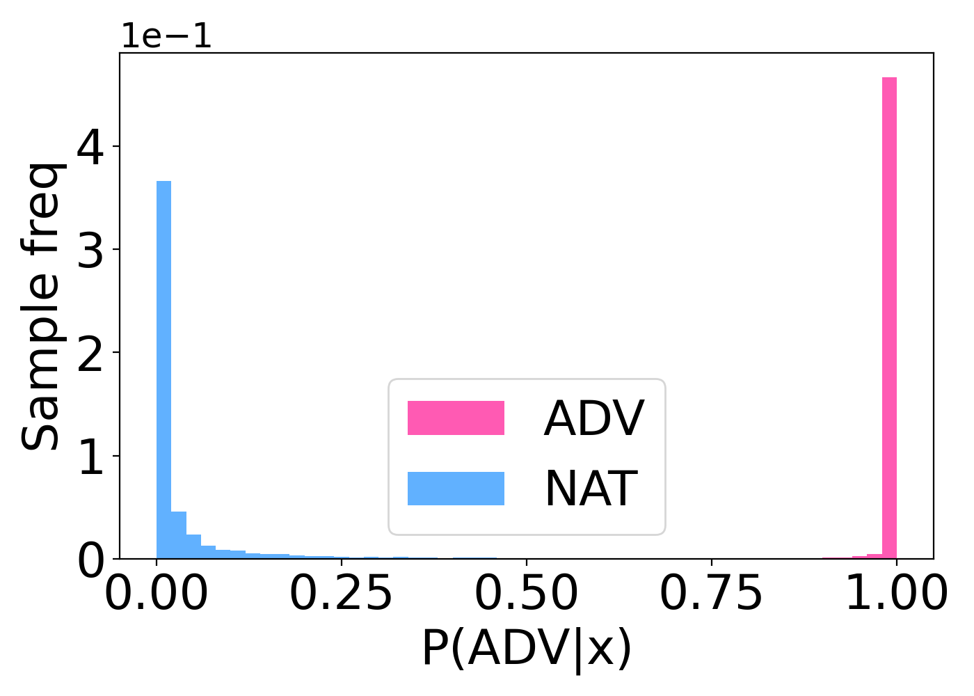
(a) PGD-L₁-40-ACE

(b) PGD-L₁-40-KL

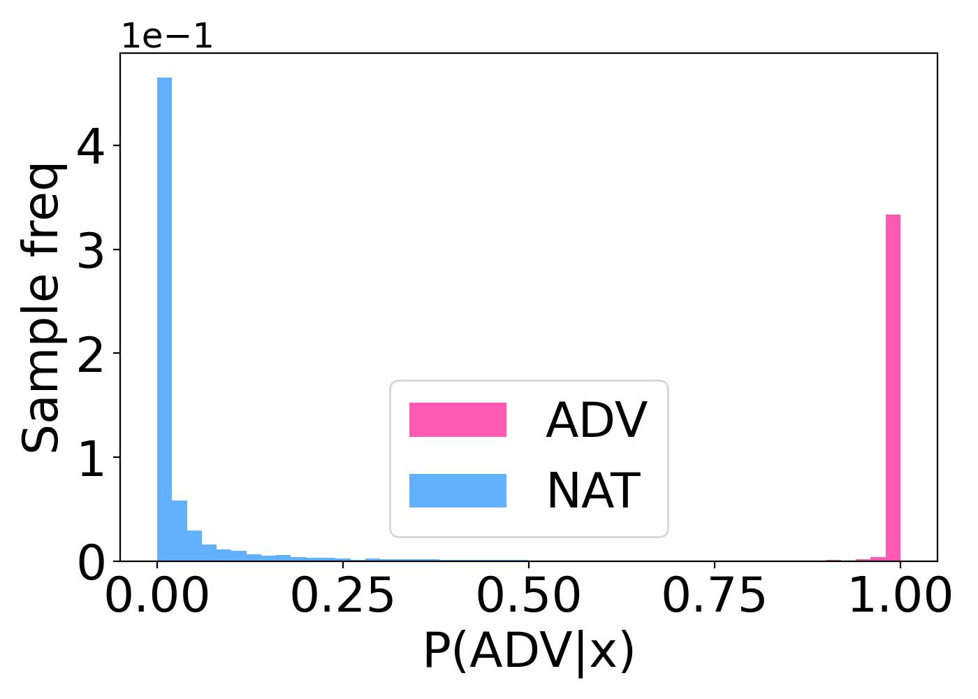
(c) PGD-L₁-40-FR

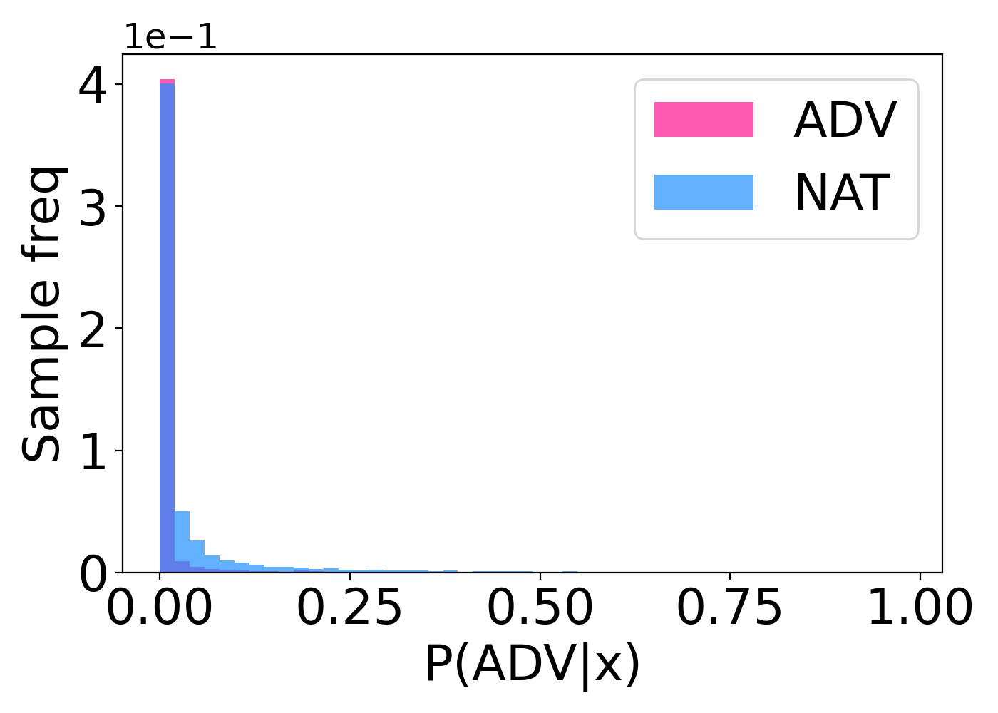
(d) PGD-L₁-40-Gini

Figure 5: In pink the results for the adversarial examples and in blue the ones for the naturals. In this simulation, we consider a subset of the available detectors (ACE, KL, FR). Under each plot, we indicate the tested attack configuration parameters: algorithm-L_p-$\varepsilon$-loss.

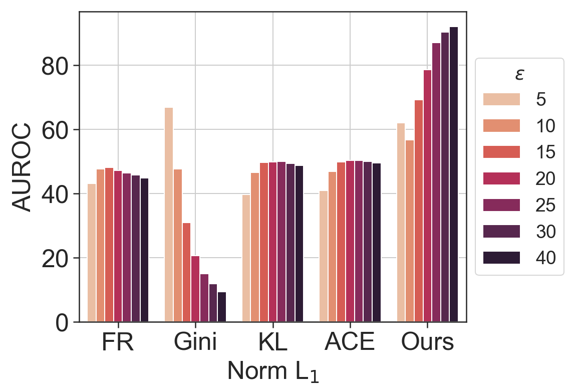
(a)

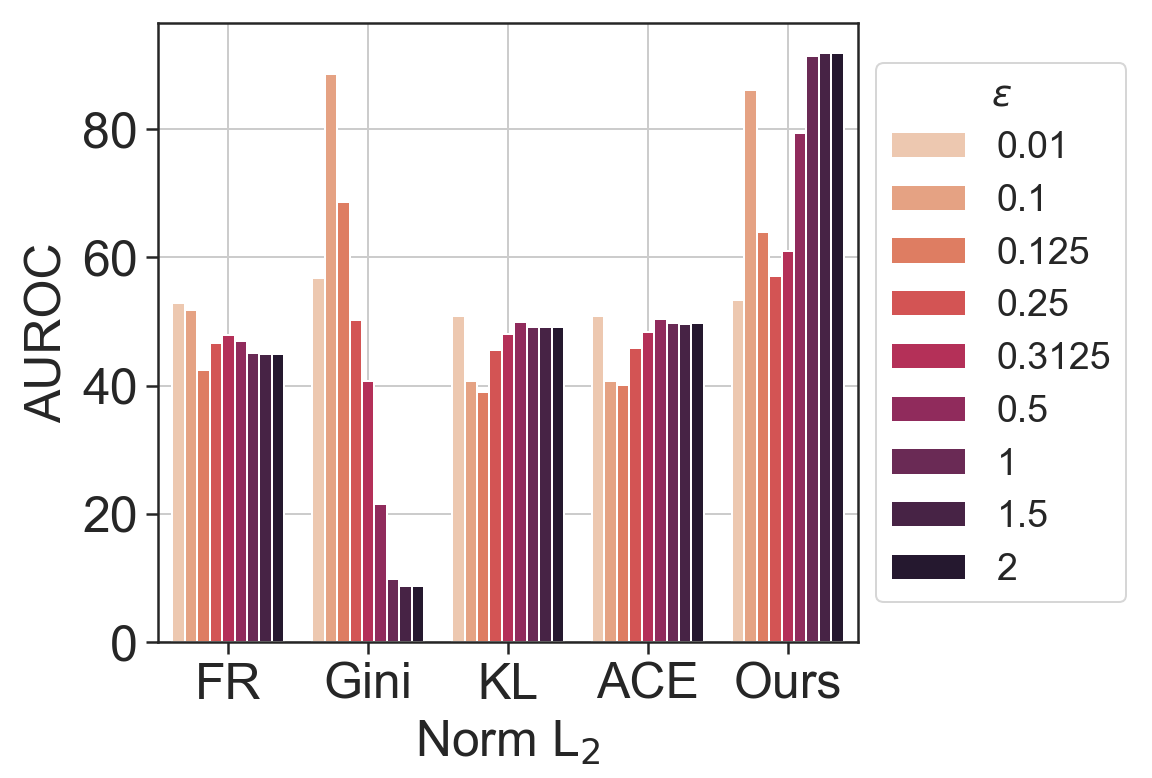
(b)

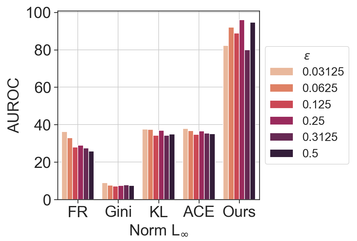
(c)

Figure 6: Performance of the various detectors grouped by L_p-norm and perturbation magnitude $\varepsilon$ on CIFAR10. Each shallow detector is named after the loss function used to craft the attacks they it is trained to detect. The plot shows how our method consistently attains better performance than the single one on all the different adversarial attacks, supporting the claim of optimality in Sec. 2.

B.6 Evaluation of the Proposed Solution in the Optimal Setting

B.6.1 Ablation Study

In Tabs. 7, 7, 9, 9, 11 and 11 we provide the complete set of results for the theoretical setting applied to CIFAR10. Additionally, the Tabs. 13, 13, 15, 15, 17 and 17 include the results for SVHN. Notice that, we include the results for all the possible combinations of the detectors in the pool.

Table 6: Theoretical framework setting: CIFAR10, PGD algorithm, $\varepsilon=0.03125$, L_∞ norm.

Pool of detectors	Attacks	AUROC$\uparrow$%	FPR$\downarrow_{95\%}$%
NSS	ACE+KL	91.0	35.0
ACE+KL	ACE+KL	99.9	0.0
ACE+KL+NSS	ACE+KL	99.9	0.2
NSS	ACE+FR	91.1	34.8
ACE+FR	ACE+FR	99.9	0.0
ACE+FR+NSS	ACE+FR	99.9	0.3
NSS	ACE+Gini	88.7	43.6
ACE+Gini	ACE+Gini	96.0	17.6
ACE+Gini+NSS	ACE+Gini	95.7	15.7
NSS	KL+FR	91.0	35.5
KL+FR	KL+FR	99.9	0.0
KL+FR+NSS	KL+FR	99.9	0.4
NSS	KL+Gini	88.7	44.3
KL+Gini	KL+Gini	95.4	18.7
KL+Gini+NSS	KL+Gini	94.9	16.9
NSS	FR+Gini	88.7	44.0
FR+Gini	FR+Gini	93.4	21.9
FR+Gini+NSS	FR+Gini	93.0	19.2
NSS	ACE+KL+FR	90.1	37.6
ACE+KL+FR	ACE+KL+FR	99.9	0.0
ACE+KL+FR+NSS	ACE+KL+FR	99.9	0.3
NSS	ACE+KL+Gini	87.8	45.5
ACE+KL+Gini	ACE+KL+Gini	95.9	17.8
ACE+KL+Gini+NSS	ACE+KL+Gini	95.6	16.0
NSS	KL+FR+Gini	88.0	45.4
KL+FR+Gini	KL+FR+Gini	95.1	19.7
KL+FR+Gini+NSS	KL+FR+Gini	94.7	17.4
NSS	ACE+KL+FR+Gini	87.3	46.7
ACE+KL+FR+Gini	ACE+KL+FR+Gini	95.6	18.8
ACE+KL+FR+Gini+NSS	ACE+KL+FR+Gini	95.3	16.5

Table 7: Theoretical framework setting: CIFAR10, PGD algorithm, $\varepsilon=0.0625$, L_∞ norm.

Pool of detectors	Attacks	AUROC$\uparrow$%	FPR$\downarrow_{95\%}$%
NSS	ACE+KL	98.9	4.3
ACE+KL	ACE+KL	100.0	0.0
ACE+KL+NSS	ACE+KL	100.0	0.0
NSS	ACE+FR	98.9	4.2
ACE+FR	ACE+FR	100.0	0.0
ACE+FR+NSS	ACE+FR	100.0	0.0
NSS	ACE+Gini	98.0	8.1
ACE+Gini	ACE+Gini	97.7	7.2
ACE+Gini+NSS	ACE+Gini	97.6	5.8
NSS	KL+FR	98.9	4.3
KL+FR	KL+FR	100.0	0.0
KL+FR+NSS	KL+FR	100.0	0.0
NSS	KL+Gini	98.0	8.3
KL+Gini	KL+Gini	97.2	7.7
KL+Gini+NSS	KL+Gini	96.8	6.6
NSS	FR+Gini	98.0	8.1
FR+Gini	FR+Gini	95.4	10.1
FR+Gini+NSS	FR+Gini	95.5	8.1
NSS	ACE+KL+FR	98.7	4.9
ACE+KL+FR	ACE+KL+FR	100.0	0.0
ACE+KL+FR+NSS	ACE+KL+FR	100.0	0.0
NSS	ACE+KL+Gini	97.9	8.6
ACE+KL+Gini	ACE+KL+Gini	97.5	7.4
ACE+KL+Gini+NSS	ACE+KL+Gini	97.3	6.1
NSS	KL+FR+Gini	97.9	8.6
KL+FR+Gini	KL+FR+Gini	96.9	8.3
KL+FR+Gini+NSS	KL+FR+Gini	96.6	6.9
NSS	ACE+KL+FR+Gini	97.8	8.9
ACE+KL+FR+Gini	ACE+KL+FR+Gini	97.3	8.0
ACE+KL+FR+Gini+NSS	ACE+KL+FR+Gini	97.1	6.3

Table 8: Theoretical framework setting: CIFAR10, PGD algorithm, $\varepsilon=0.125$, L_∞ norm.

Pool of detectors	Attacks	AUROC$\uparrow$%	FPR$\downarrow_{95\%}$%
NSS	ACE+KL	99.7	0.6
ACE+KL	ACE+KL	100.0	0.0
ACE+KL+NSS	ACE+KL	100.0	0.0
NSS	ACE+FR	99.6	0.6
ACE+FR	ACE+FR	100.0	0.0
ACE+FR+NSS	ACE+FR	100.0	0.0
NSS	ACE+Gini	99.6	0.6
ACE+Gini	ACE+Gini	97.1	7.3
ACE+Gini+NSS	ACE+Gini	97.3	3.2
NSS	KL+FR	99.6	0.6
KL+FR	KL+FR	100.0	0.0
KL+FR+NSS	KL+FR	100.0	0.0
NSS	KL+Gini	99.6	0.6
KL+Gini	KL+Gini	96.9	7.3
KL+Gini+NSS	KL+Gini	97.2	3.1
NSS	FR+Gini	99.6	0.6
FR+Gini	FR+Gini	95.3	9.4
FR+Gini+NSS	FR+Gini	96.1	4.2
NSS	ACE+KL+FR	99.6	0.6
ACE+KL+FR	ACE+KL+FR	100.0	0.0
ACE+KL+FR+NSS	ACE+KL+FR	100.0	0.0
NSS	ACE+KL+Gini	99.6	0.6
ACE+KL+Gini	ACE+KL+Gini	97.2	7.2
ACE+KL+Gini+NSS	ACE+KL+Gini	97.3	3.1
NSS	KL+FR+Gini	99.6	0.6
KL+FR+Gini	KL+FR+Gini	96.6	8.0
KL+FR+Gini+NSS	KL+FR+Gini	97.0	3.3
NSS	ACE+KL+FR+Gini	99.6	0.6
ACE+KL+FR+Gini	ACE+KL+FR+Gini	96.8	7.8
ACE+KL+FR+Gini+NSS	ACE+KL+FR+Gini	97.1	3.2

Table 9: Theoretical framework setting: CIFAR10, PGD algorithm, $\varepsilon=0.25$, L_∞ norm.

Pool of detectors	Attacks	AUROC$\uparrow$%	FPR$\downarrow_{95\%}$%
NSS	ACE+KL	99.7	0.6
ACE+KL	ACE+KL	100.0	0.0
ACE+KL+NSS	ACE+KL	100.0	0.0
NSS	ACE+FR	99.7	0.6
ACE+FR	ACE+FR	100.0	0.0
ACE+FR+NSS	ACE+FR	100.0	0.0
NSS	ACE+Gini	99.6	0.6
ACE+Gini	ACE+Gini	97.2	7.2
ACE+Gini+NSS	ACE+Gini	97.6	2.8
NSS	KL+FR	99.7	0.6
KL+FR	KL+FR	100.0	0.0
KL+FR+NSS	KL+FR	100.0	0.0
NSS	KL+Gini	99.6	0.6
KL+Gini	KL+Gini	96.4	7.7
KL+Gini+NSS	KL+Gini	96.6	3.8
NSS	FR+Gini	99.6	0.6
FR+Gini	FR+Gini	95.1	9.5
FR+Gini+NSS	FR+Gini	96.1	4.2
NSS	ACE+KL+FR	99.7	0.6
ACE+KL+FR	ACE+KL+FR	100.0	0.0
ACE+KL+FR+NSS	ACE+KL+FR	100.0	0.0
NSS	ACE+KL+Gini	99.6	0.6
ACE+KL+Gini	ACE+KL+Gini	96.9	7.4
ACE+KL+Gini+NSS	ACE+KL+Gini	97.1	3.3
NSS	KL+FR+Gini	99.6	0.6
KL+FR+Gini	KL+FR+Gini	96.1	8.4
KL+FR+Gini+NSS	KL+FR+Gini	96.4	4.0
NSS	ACE+KL+FR+Gini	99.6	0.6
ACE+KL+FR+Gini	ACE+KL+FR+Gini	96.5	8.1
ACE+KL+FR+Gini+NSS	ACE+KL+FR+Gini	96.8	3.5

Table 10: Theoretical framework setting: CIFAR10, PGD algorithm, $\varepsilon=0.3125$, L_∞ norm.

Pool of detectors	Attacks	AUROC$\uparrow$%	FPR$\downarrow_{95\%}$%
NSS	ACE+KL	99.7	0.6
ACE+KL	ACE+KL	100.0	0.0
ACE+KL+NSS	ACE+KL	100.0	0.0
NSS	ACE+FR	99.7	0.6
ACE+FR	ACE+FR	100.0	0.0
ACE+FR+NSS	ACE+FR	100.0	0.0
NSS	ACE+Gini	99.7	0.6
ACE+Gini	ACE+Gini	96.9	7.4
ACE+Gini+NSS	ACE+Gini	97.4	3.1
NSS	KL+FR	99.7	0.6
KL+FR	KL+FR	100.0	0.0
KL+FR+NSS	KL+FR	100.0	0.0
NSS	KL+Gini	99.7	0.6
KL+Gini	KL+Gini	96.3	7.9
KL+Gini+NSS	KL+Gini	96.4	4.1
NSS	FR+Gini	99.6	0.6
FR+Gini	FR+Gini	95.1	9.6
FR+Gini+NSS	FR+Gini	96.1	4.2
NSS	ACE+KL+FR	99.7	0.6
ACE+KL+FR	ACE+KL+FR	100.0	0.0
ACE+KL+FR+NSS	ACE+KL+FR	100.0	0.0
NSS	ACE+KL+Gini	99.7	0.6
ACE+KL+Gini	ACE+KL+Gini	96.7	7.6
ACE+KL+Gini+NSS	ACE+KL+Gini	96.8	3.7
NSS	KL+FR+Gini	99.6	0.6
KL+FR+Gini	KL+FR+Gini	95.9	8.6
KL+FR+Gini+NSS	KL+FR+Gini	96.1	4.3
NSS	ACE+KL+FR+Gini	99.6	0.6
ACE+KL+FR+Gini	ACE+KL+FR+Gini	96.3	8.2
ACE+KL+FR+Gini+NSS	ACE+KL+FR+Gini	96.5	3.8

Table 11: Theoretical framework setting: CIFAR10, PGD algorithm, $\varepsilon=0.5$, L_∞ norm.

Pool of detectors	Attacks	AUROC$\uparrow$%	FPR$\downarrow_{95\%}$%
NSS	ACE+KL	99.7	0.6
ACE+KL	ACE+KL	100.0	0.0
ACE+KL+NSS	ACE+KL	100.0	0.0
NSS	ACE+FR	99.7	0.6
ACE+FR	ACE+FR	100.0	0.0
ACE+FR+NSS	ACE+FR	100.0	0.0
NSS	ACE+Gini	99.7	0.6
ACE+Gini	ACE+Gini	97.0	7.4
ACE+Gini+NSS	ACE+Gini	97.5	3.0
NSS	KL+FR	99.7	0.6
KL+FR	KL+FR	100.0	0.0
KL+FR+NSS	KL+FR	100.0	0.0
NSS	KL+Gini	99.6	0.6
KL+Gini	KL+Gini	96.5	7.7
KL+Gini+NSS	KL+Gini	96.7	3.7
NSS	FR+Gini	99.6	0.6
FR+Gini	FR+Gini	95.1	9.6
FR+Gini+NSS	FR+Gini	96.1	4.2
NSS	ACE+KL+FR	99.7	0.6
ACE+KL+FR	ACE+KL+FR	100.0	0.0
ACE+KL+FR+NSS	ACE+KL+FR	100.0	0.0
NSS	ACE+KL+Gini	99.6	0.6
ACE+KL+Gini	ACE+KL+Gini	96.9	7.4
ACE+KL+Gini+NSS	ACE+KL+Gini	97.2	3.3
NSS	KL+FR+Gini	99.6	0.6
KL+FR+Gini	KL+FR+Gini	96.1	8.4
KL+FR+Gini+NSS	KL+FR+Gini	96.5	3.9
NSS	ACE+KL+FR+Gini	99.6	0.6
ACE+KL+FR+Gini	ACE+KL+FR+Gini	96.5	8.1
ACE+KL+FR+Gini+NSS	ACE+KL+FR+Gini	96.9	3.4

Table 12: Theoretical framework setting: SVHN, PGD algorithm, $\varepsilon=0.03125$, L_∞ norm.

Pool of detectors	Attacks	AUROC$\uparrow$%	FPR$\downarrow_{95\%}$%
NSS	ACE+KL	90.0	0.9
ACE+KL	ACE+KL	97.4	13.5
ACE+KL+NSS	ACE+KL	99.3	0.5
NSS	ACE+FR	90.0	0.9
ACE+FR	ACE+FR	97.4	12.9
ACE+FR+NSS	ACE+FR	99.2	0.5
NSS	ACE+Gini	89.0	1.9
ACE+Gini	ACE+Gini	91.6	24.9
ACE+Gini+NSS	ACE+Gini	90.2	14.0
NSS	KL+FR	90.0	0.9
KL+FR	KL+FR	97.6	11.2
KL+FR+NSS	KL+FR	99.3	0.5
NSS	KL+Gini	89.0	1.9
KL+Gini	KL+Gini	92.8	15.0
KL+Gini+NSS	KL+Gini	95.4	8.9
NSS	FR+Gini	89.1	1.9
FR+Gini	FR+Gini	92.5	15.3
FR+Gini+NSS	FR+Gini	95.1	9.0
NSS	ACE+KL+FR	89.9	1.0
ACE+KL+FR	ACE+KL+FR	97.3	14.7
ACE+KL+FR+NSS	ACE+KL+FR	99.2	0.6
NSS	ACE+KL+Gini	88.9	2.0
ACE+KL+Gini	ACE+KL+Gini	91.8	25.7
ACE+KL+Gini+NSS	ACE+KL+Gini	89.3	14.8
NSS	KL+FR+Gini	89.0	2.0
KL+FR+Gini	KL+FR+Gini	92.5	18.7
KL+FR+Gini+NSS	KL+FR+Gini	91.9	12.3
NSS	ACE+KL+FR+Gini	88.8	2.1
ACE+KL+FR+Gini	ACE+KL+FR+Gini	91.9	25.9
ACE+KL+FR+Gini+NSS	ACE+KL+FR+Gini	88.9	15.2

Table 13: Theoretical framework setting: SVHN, PGD algorithm, $\varepsilon=0.0625$, L_∞ norm.

Pool of detectors	Attacks	AUROC$\uparrow$%	FPR$\downarrow_{95\%}$%
NSS	ACE+KL	91.3	0.0
ACE+KL	ACE+KL	99.9	0.0
ACE+KL+NSS	ACE+KL	100.0	0.0
NSS	ACE+FR	91.3	0.0
ACE+FR	ACE+FR	99.9	0.0
ACE+FR+NSS	ACE+FR	100.0	0.0
NSS	ACE+Gini	91.2	0.0
ACE+Gini	ACE+Gini	94.7	6.0
ACE+Gini+NSS	ACE+Gini	89.5	10.9
NSS	KL+FR	91.3	0.0
KL+FR	KL+FR	99.9	0.0
KL+FR+NSS	KL+FR	100.0	0.0
NSS	KL+Gini	91.2	0.0
KL+Gini	KL+Gini	94.4	6.1
KL+Gini+NSS	KL+Gini	99.6	0.9
NSS	FR+Gini	91.2	0.0
FR+Gini	FR+Gini	93.6	7.0
FR+Gini+NSS	FR+Gini	94.5	10.0
NSS	ACE+KL+FR	91.3	0.0
ACE+KL+FR	ACE+KL+FR	99.9	0.0
ACE+KL+FR+NSS	ACE+KL+FR	100.0	0.0
NSS	ACE+KL+Gini	91.2	0.0
ACE+KL+Gini	ACE+KL+Gini	95.0	5.7
ACE+KL+Gini+NSS	ACE+KL+Gini	87.9	12.4
NSS	KL+FR+Gini	91.2	0.0
KL+FR+Gini	KL+FR+Gini	94.4	6.0
KL+FR+Gini+NSS	KL+FR+Gini	92.4	12.4
NSS	ACE+KL+FR+Gini	91.2	0.0
ACE+KL+FR+Gini	ACE+KL+FR+Gini	94.6	6.0
ACE+KL+FR+Gini+NSS	ACE+KL+FR+Gini	87.4	13.0

Table 14: Theoretical framework setting: SVHN, PGD algorithm, $\varepsilon=0.125$, L_∞ norm.

Pool of detectors	Attacks	AUROC$\uparrow$%	FPR$\downarrow_{95\%}$%
NSS	ACE+KL	91.3	0.0
ACE+KL	ACE+KL	100.0	0.0
ACE+KL+NSS	ACE+KL	100.0	0.0
NSS	ACE+FR	91.3	0.0
ACE+FR	ACE+FR	100.0	0.0
ACE+FR+NSS	ACE+FR	100.0	0.0
NSS	ACE+Gini	91.3	0.0
ACE+Gini	ACE+Gini	94.8	5.6
ACE+Gini+NSS	ACE+Gini	99.7	0.4
NSS	KL+FR	91.3	0.0
KL+FR	KL+FR	100.0	0.0
KL+FR+NSS	KL+FR	100.0	0.0
NSS	KL+Gini	91.3	0.0
KL+Gini	KL+Gini	94.5	6.1
KL+Gini+NSS	KL+Gini	99.6	0.9
NSS	FR+Gini	91.3	0.0
FR+Gini	FR+Gini	93.7	7.0
FR+Gini+NSS	FR+Gini	94.6	10.0
NSS	ACE+KL+FR	91.3	0.0
ACE+KL+FR	ACE+KL+FR	100.0	0.0
ACE+KL+FR+NSS	ACE+KL+FR	100.0	0.0
NSS	ACE+KL+Gini	91.3	0.0
ACE+KL+Gini	ACE+KL+Gini	95.2	5.4
ACE+KL+Gini+NSS	ACE+KL+Gini	97.8	2.5
NSS	KL+FR+Gini	91.3	0.0
KL+FR+Gini	KL+FR+Gini	94.6	6.0
KL+FR+Gini+NSS	KL+FR+Gini	93.4	12.4
NSS	ACE+KL+FR+Gini	91.3	0.0
ACE+KL+FR+Gini	ACE+KL+FR+Gini	94.8	6.0
ACE+KL+FR+Gini+NSS	ACE+KL+FR+Gini	92.5	13.0

Table 15: Theoretical framework setting: SVHN, PGD algorithm, $\varepsilon=0.25$, L_∞ norm.

Pool of detectors	Attacks	AUROC$\uparrow$%	FPR$\downarrow_{95\%}$%
NSS	ACE+KL	91.3	0.0
ACE+KL	ACE+KL	100.0	0.0
ACE+KL+NSS	ACE+KL	100.0	0.0
NSS	ACE+FR	91.3	0.0
ACE+FR	ACE+FR	100.0	0.0
ACE+FR+NSS	ACE+FR	100.0	0.0
NSS	ACE+Gini	91.3	0.0
ACE+Gini	ACE+Gini	94.8	5.6
ACE+Gini+NSS	ACE+Gini	99.7	0.4
NSS	KL+FR	91.3	0.0
KL+FR	KL+FR	100.0	0.0
KL+FR+NSS	KL+FR	100.0	0.0
NSS	KL+Gini	91.3	0.0
KL+Gini	KL+Gini	94.5	6.1
KL+Gini+NSS	KL+Gini	99.6	0.9
NSS	FR+Gini	91.3	0.0
FR+Gini	FR+Gini	93.7	7.0
FR+Gini+NSS	FR+Gini	94.7	10.0
NSS	ACE+KL+FR	91.3	0.0
ACE+KL+FR	ACE+KL+FR	100.0	0.0
ACE+KL+FR+NSS	ACE+KL+FR	100.0	0.0
NSS	ACE+KL+Gini	91.3	0.0
ACE+KL+Gini	ACE+KL+Gini	95.2	5.3
ACE+KL+Gini+NSS	ACE+KL+Gini	99.7	0.4
NSS	KL+FR+Gini	91.3	0.0
KL+FR+Gini	KL+FR+Gini	94.6	6.0
KL+FR+Gini+NSS	KL+FR+Gini	93.5	12.4
NSS	ACE+KL+FR+Gini	91.3	0.0
ACE+KL+FR+Gini	ACE+KL+FR+Gini	94.8	6.0
ACE+KL+FR+Gini+NSS	ACE+KL+FR+Gini	93.5	13.0

Table 16: Theoretical framework setting: SVHN, PGD algorithm, $\varepsilon=0.3125$, L_∞ norm.

Pool of detectors	Attacks	AUROC$\uparrow$%	FPR$\downarrow_{95\%}$%
NSS	ACE+KL	91.3	0.0
ACE+KL	ACE+KL	100.0	0.0
ACE+KL+NSS	ACE+KL	100.0	0.0
NSS	ACE+FR	91.3	0.0
ACE+FR	ACE+FR	100.0	0.0
ACE+FR+NSS	ACE+FR	100.0	0.0
NSS	ACE+Gini	91.3	0.0
ACE+Gini	ACE+Gini	94.8	5.6
ACE+Gini+NSS	ACE+Gini	99.7	0.4
NSS	KL+FR	91.3	0.0
KL+FR	KL+FR	100.0	0.0
KL+FR+NSS	KL+FR	100.0	0.0
NSS	KL+Gini	91.3	0.0
KL+Gini	KL+Gini	94.5	6.1
KL+Gini+NSS	KL+Gini	99.6	0.9
NSS	FR+Gini	91.3	0.0
FR+Gini	FR+Gini	93.7	7.0
FR+Gini+NSS	FR+Gini	94.7	10.0
NSS	ACE+KL+FR	91.3	0.0
ACE+KL+FR	ACE+KL+FR	100.0	0.0
ACE+KL+FR+NSS	ACE+KL+FR	100.0	0.0
NSS	ACE+KL+Gini	91.3	0.0
ACE+KL+Gini	ACE+KL+Gini	95.2	5.4
ACE+KL+Gini+NSS	ACE+KL+Gini	99.7	0.4
NSS	KL+FR+Gini	91.3	0.0
KL+FR+Gini	KL+FR+Gini	94.6	6.0
KL+FR+Gini+NSS	KL+FR+Gini	93.5	12.4
NSS	ACE+KL+FR+Gini	91.3	0.0
ACE+KL+FR+Gini	ACE+KL+FR+Gini	94.8	6.0
ACE+KL+FR+Gini+NSS	ACE+KL+FR+Gini	93.5	13.0

Table 17: Theoretical framework setting: SVHN, PGD algorithm, $\varepsilon=0.5$, L_∞ norm.

Pool of detectors	Attacks	AUROC$\uparrow$%	FPR$\downarrow_{95\%}$%
NSS	ACE+KL	91.3	0.0
ACE+KL	ACE+KL	100.0	0.0
ACE+KL+NSS	ACE+KL	100.0	0.0
NSS	ACE+FR	91.3	0.0
ACE+FR	ACE+FR	100.0	0.0
ACE+FR+NSS	ACE+FR	100.0	0.0
NSS	ACE+Gini	91.3	0.0
ACE+Gini	ACE+Gini	94.8	5.6
ACE+Gini+NSS	ACE+Gini	99.7	0.4
NSS	KL+FR	91.3	0.0
KL+FR	KL+FR	100.0	0.0
KL+FR+NSS	KL+FR	100.0	0.0
NSS	KL+Gini	91.3	0.0
KL+Gini	KL+Gini	94.5	6.1
KL+Gini+NSS	KL+Gini	99.6	0.9
NSS	FR+Gini	91.3	0.0
FR+Gini	FR+Gini	93.7	7.0
FR+Gini+NSS	FR+Gini	94.7	10.0
NSS	ACE+KL+FR	91.3	0.0
ACE+KL+FR	ACE+KL+FR	100.0	0.0
ACE+KL+FR+NSS	ACE+KL+FR	100.0	0.0
NSS	ACE+KL+Gini	91.3	0.0
ACE+KL+Gini	ACE+KL+Gini	95.2	5.3
ACE+KL+Gini+NSS	ACE+KL+Gini	99.7	0.4
NSS	KL+FR+Gini	91.3	0.0
KL+FR+Gini	KL+FR+Gini	94.6	6.0
KL+FR+Gini+NSS	KL+FR+Gini	93.5	12.4
NSS	ACE+KL+FR+Gini	91.3	0.0
ACE+KL+FR+Gini	ACE+KL+FR+Gini	94.8	6.0
ACE+KL+FR+Gini+NSS	ACE+KL+FR+Gini	93.5	13.0

B.7 Evaluation of the Proposed Solution in the Setting of [Granese et al., 2022]

Table 18: Comparison between the proposed method and NSS on CIFAR10 and SVHN. The ^⋆ symbol means the perturbation mechanism is executed in parallel four times starting from the same original clean sample, each time using one of the objective losses between ACE Eq. (3), KL Eq. (4), FR Eq. (5), or Eq. (6) in [Granese et al., 2022].

	CIFAR10						SVHN
	NSS			Ours			NSS			Ours
	AUROC$\uparrow$%	FPR$\downarrow_{95\%}$%		AUROC$\uparrow$%	FPR$\downarrow_{95\%}$%		AUROC$\uparrow$%	FPR$\downarrow_{95\%}$%		AUROC$\uparrow$%	FPR$\downarrow_{95\%}$%
Norm L1
PGD1⋆
$\varepsilon=5$	48.5	94.2		62.1	87.1		40.2	91.3		76.9	78.9
$\varepsilon=10$	54.0	90.3		56.8	90.4		36.9	91.3		73.0	82.7
$\varepsilon=15$	58.8	86.8		69.3	84.4		35.6	91.3		78.9	72.5
$\varepsilon=20$	63.5	82.3		78.7	73.1		36.1	91.3		83.6	60.6
$\varepsilon=25$	67.7	77.2		87.1	50.8		37.8	91.3		87.0	48.7
$\varepsilon=30$	71.4	73.4		90.3	35.4		39.8	91.3		89.3	37.2
$\varepsilon=40$	76.1	67.3		92.1	26.4		43.1	91.3		92.7	20.0
Norm L2
PGD2⋆
$\varepsilon=0.125$	48.3	94.3		63.9	85.3		40.8	91.3		80.2	74.6
$\varepsilon=0.25$	53.2	91.2		57.2	90.3		37.2	91.3		74.1	81.6
$\varepsilon=0.3125$	55.8	89.2		61.0	88.8		36.1	91.3		75.1	79.7
$\varepsilon=0.5$	63.3	82.6		79.4	73.0		35.9	91.3		82.5	64.4
$\varepsilon=1$	76.4	67.5		91.4	26.3		42.5	91.3		92.3	24.6
$\varepsilon=1.5$	81.0	63.0		91.9	24.3		46.3	91.3		94.1	7.5
$\varepsilon=2$	82.6	62.3		91.9	24.2		49.8	91.3		94.9	5.3
DeepFool
No $\varepsilon$	57.0	91.7		82.3	53.7		41.3	91.3		94.9	12.0
CW2
$\varepsilon=0.01$	56.4	90.8		53.4	92.3		41.0	91.3		54.2	92.0
HOP
$\varepsilon=0.1$	66.1	87.0		86.1	49.0		67.6	84.2		96.0	10.2
Norm L∞
PGDi⋆, FGSM⋆, BIM⋆
$\varepsilon=0.03125$	83.0	55.3		82.3	59.8		86.3	46.9		81.4	64.8
$\varepsilon=0.0625$	96.0	17.2		92.0	29.6		88.9	0.7		89.1	33.3
$\varepsilon=0.25$	97.3	0.6		95.9	8.8		51.6	88.9		92.3	16.4
$\varepsilon=0.5$	82.5	100.0		94.6	9.7		46.7	86.7		92.9	14.4
PGDi⋆, FGSM⋆, BIM⋆, SA
$\varepsilon=0.125$	9.4	99.9		88.9	40.8		32.9	91.3		89.2	29.0
PGDi⋆, FGSM⋆, BIM⋆, CWi
$\varepsilon=0.3125$	63.2	99.1		80.0	61.2		41.3	91.3		88.2	33.1
No norm
STA
No $\varepsilon$	88.5	38.8		82.7	52.4		91.2	0.2		90.2	23.2

B.7.1 Ablation Study

As a final set of experiments, we examine how the combinations of detectors affect the aggregator’s performance. Differently from the ablation study in Sec. B.6.1, the set of attacks is always fixed as in Tab. 1. Therefore, we consider all the possible combinations ($2^{5}=32$) of the detectors discussed throughout this paper. In Fig. 7, the set of detectors to aggregate is shown on the vertical axis, and the average AUROC is shown on the horizontal axis. The results are computed over all the attacks grouped w.r.t. the L_p norm used. Figure 7 shows that the Gini detector is a necessary but not sufficient detector to include in the pool: the combination of the Gini detector with even just one other detector yielded unexpected results, despite its low effectiveness when considered in isolation (cf. Figs. 7(j), 7(k) and 7(l)). This suggests that having mutually-exclusive detector (i.e., a detector that is designed to recognize a specific typology of attack) in our aggregator would be actually beneficial for the detection task. Note that, in this sense, parallelism can be created with the work in [Abdelnabi and Fritz, 2021] where the authors propose a new training approach based on adversarially-disjointed models with minimal transferability of the attacks.

(a) Attacks created with L₁

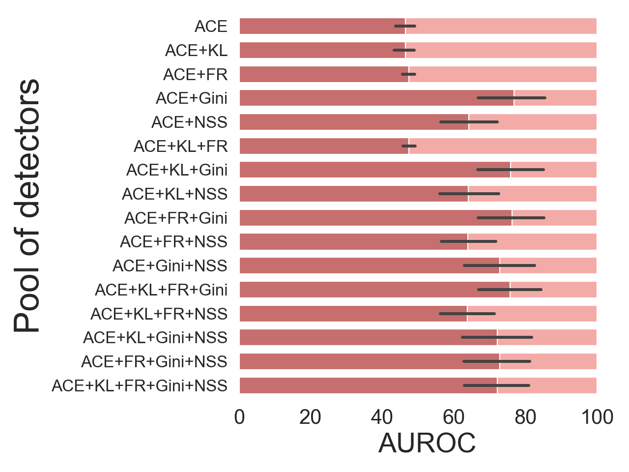
(b) Attacks created with L₂

(c) Attacks created with L_∞

(d) Attacks created with L₁

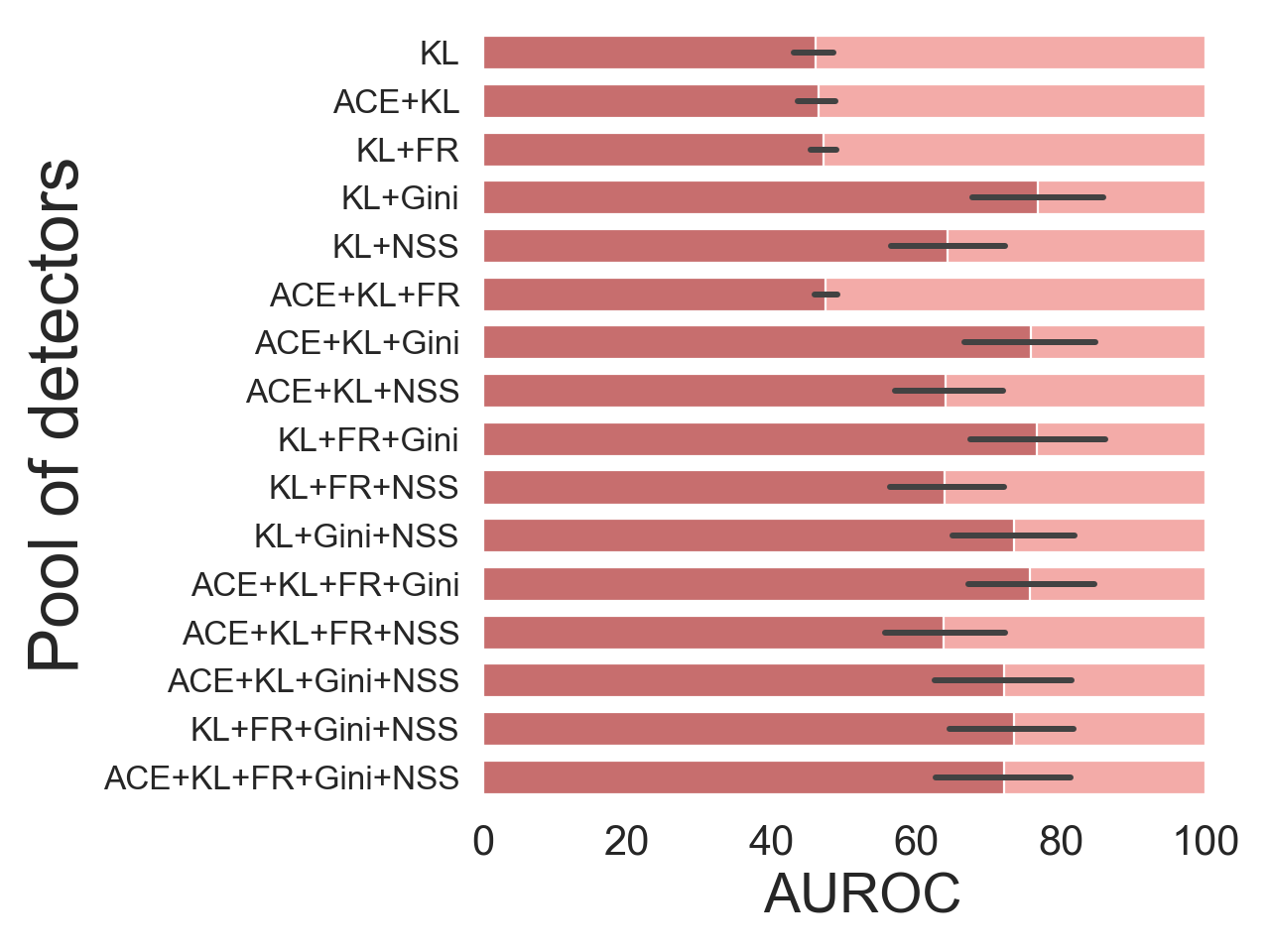
(e) Attacks created with L₂

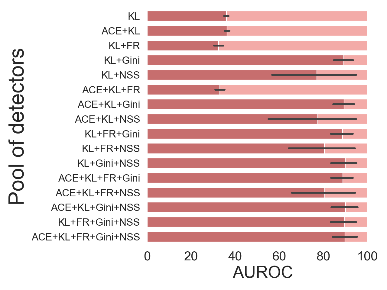
(f) Attacks created with L_∞

(g) Attacks created with L₁

(h) Attacks created with L₂

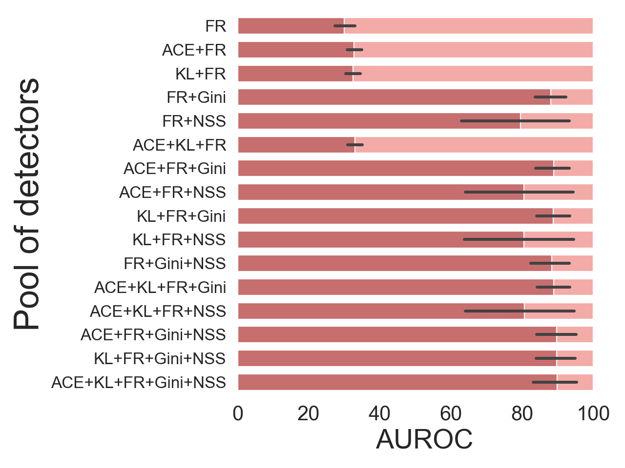
(i) Attacks created with L_∞

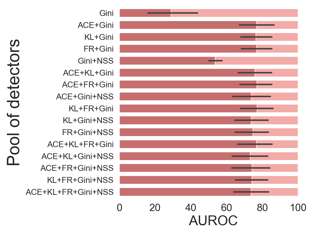
(j) Attacks created with L₁

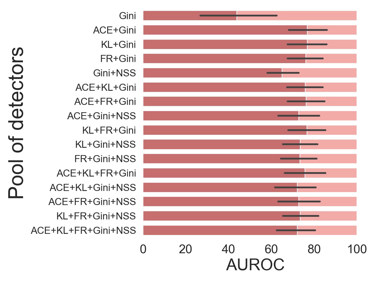
(k) Attacks created with L₂

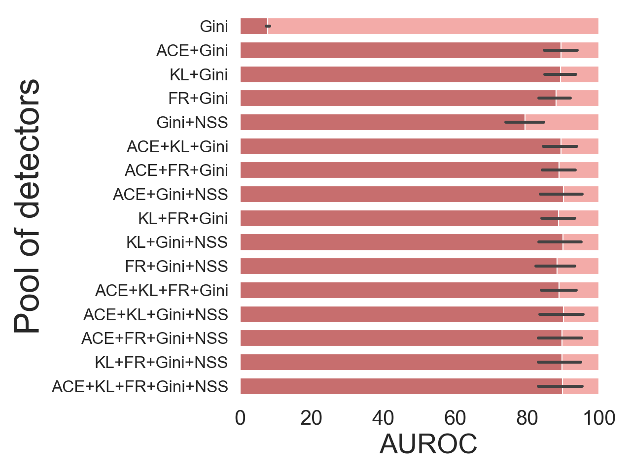
(l) Attacks created with L_∞

(m) Attacks created with L₁

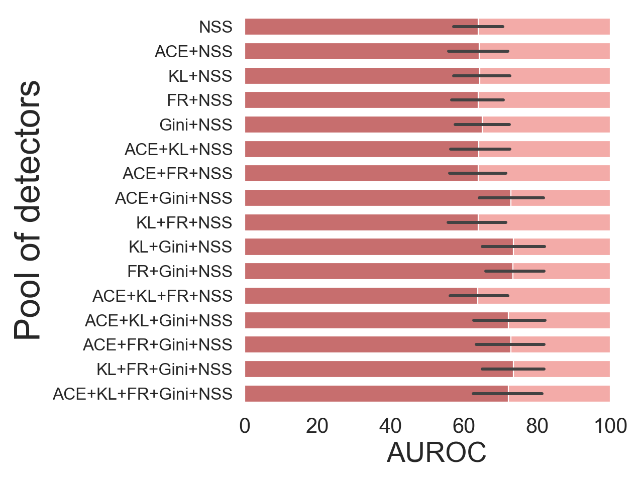
(n) Attacks created with L₂

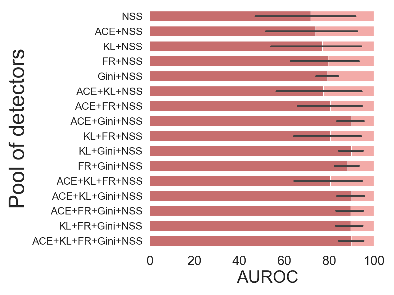
(o) Attacks created with L_∞

Figure 7: Ablation study: Mead setting.

B.8 Evaluation of the Proposed Solution in the Single-Armed Setting

In these experiments, we move from the multi-armed adversarial attack scenario if [Granese et al., 2022], to the single-armed setting where the different detectors are aggregated to detect one single attack at a time. Note that, in this case, we do not impose any constraints on the relationship between detectors and attacks. As we follow what is usually done in the literature. As a result, we may come across scenarios where none of the detectors perform optimally in recognizing certain attacks. As well as it is possible to encounter situations where multiple detectors are equally optimal for specific types of attacks. We refer to Tab. 19 for the complete set of results. Crucially, these experiments show that aggregation of the detectors can also improve the performance of detecting specific attacks. In particular, we would like to draw attention to the fact that we outperform NSS in the vast majority of the cases. Moreover, we achieve a maximum gain of 82.8 percentage points in terms of AUROC$\uparrow$% (cf. SA attack) and 97.6 percentage points in terms of FPR$\downarrow_{95\%}$% (cf. FGSM with $\varepsilon=0.5$ attack). On the other side, the competitor outperforms our proposed method only in a few cases, achieving a maximum gain of 5.9 percentage points in terms of AUROC$\uparrow$% and 27.4 percentage points in terms of FPR$\downarrow_{95\%}$% (cf. FGSM with $\varepsilon$=0.03125 attack in both the cases), and these gains are much lower than those obtained by the proposed method.

Table 19: The proposed method and NSS in the non-simultaneous setting. The column names ACE, KL, FR, and Gini denote the loss function used to craft the attacks. HOP, DeepFool, CW2, and STA attacks have already been considered individually in  Tab. 18.

	CIFAR10
	Ours AUROC$\uparrow$% (FPR$\downarrow_{95\%}$%)  –  NSS AUROC$\uparrow$% (FPR$\downarrow_{95\%}$%)
	ACE		KL		FR		Gini
PGD1
$\varepsilon=$ 5	66.2 (83.5) – 49.9 (93.5)		64.2 (85.6) – 49.6 (93.0)		63.1 (86.8) – 49.9 (93.3)		80.7 (58.4) – 50.3 (93.2)
$\varepsilon=$ 10	62.6 (87.5) – 56.9 (88.4)		62.2 (88.4) – 56.6 (88.3)		63.1 (86.5) – 57.0 (88.1)		86.9 (46.0) – 57.1 (88.8)
$\varepsilon=$ 15	74.2 (81.3) – 63.1 (83.0)		75.2 (80.5) – 62.8 (83.1)		75.3 (79.5) – 63.2 (82.5)		90.0 (37.0) – 63.5 (84.0)
$\varepsilon=$ 20	86.8 (65.3) – 68.5 (77.1)		87.5 (63.1) – 68.1 (77.3)		86.9 (63.2) – 68.7 (76.4)		91.7 (31.1) – 69.9 (77.6)
$\varepsilon=$ 25	93.9 (38.4) – 73.1 (71.1)		94.3 (36.1) – 72.7 (71.8)		93.7 (41.0) – 73.4 (70.9)		92.3 (28.9) – 75.0 (71.4)
$\varepsilon=$ 30	97.1 (12.2) – 77.1 (64.5)		97.2 (12.6) – 76.8 (65.1)		96.8 (15.9) – 77.4 (65.2)		92.6 (27.9) – 78.6 (67.3)
$\varepsilon=$ 40	98.9 (1.0) – 83.5 (52.7)		99.0 (1.0) – 83.3 (53.5)		98.8 (1.0) – 83.6 (52.7)		92.7 (27.4) – 80.1 (64.9)
PGD2
$\varepsilon=$ .125	67.9 (81.0) – 49.5 (93.8)		65.4 (84.1) – 49.1 (93.5)		63.9 (86.5) – 49.6 (93.5)		80.6 (58.4) – 49.5 (94.3)
$\varepsilon=$ .25	62.3 (87.4) – 55.9 (89.1)		62.1 (88.0) – 55.6 (89.2)		62.6 (87.6) – 55.8 (89.4)		86.7 (46.4) – 55.9 (89.8)
$\varepsilon=$ .3125	66.4 (86.2) – 59.4 (86.5)		67.0 (85.8) – 59.0 (86.6)		67.8 (84.8) – 59.3 (86.6)		88.4 (42.2) – 59.3 (87.7)
$\varepsilon=$ .5	86.4 (66.9) – 68.3 (77.4)		87.2 (64.4) – 68.0 (77.4)		86.7 (63.9) – 68.4 (77.2)		91.4 (31.4) – 69.0 (78.7)
$\varepsilon=$ 1	98.9 (0.9) – 84.4 (50.6)		99.0 (0.9) – 84.3 (50.5)		98.8 (0.9) – 84.7 (50.7)		92.5 (27.2) – 79.3 (66.8)
$\varepsilon=$ 1.5	99.2 (0.9) – 92.8 (28.7)		99.3 (0.9) – 92.7 (28.9)		99.3 (0.7) – 93.0 (27.3)		92.5 (27.2) – 79.5 (66.5)
$\varepsilon=$ 2	99.3 (0.8) – 96.8 (13.9)		99.3 (0.8) – 96.9 (13.1)		99.3 (0.9) – 95.9 (17.2)		92.5 (27.2) – 79.5 (66.5)
PGDi
$\varepsilon=$ .03125	99.1 (0.9) – 92.3 (31.0)		99.1 (0.9) – 92.1 (31.9)		99.0 (0.9) – 92.2 (30.7)		94.8 (21.5) – 89.0 (44.0)
$\varepsilon=$ .0625	99.3 (0.8) – 99.1 (3.3)		99.3 (0.8) – 99.1 (3.3)		99.3 (0.8) – 99.1 (3.6)		97.4 (8.0) – 98.1 (8.1)
$\varepsilon=$ .125	99.3 (0.7) – 99.7 (0.6)		99.3 (0.9) – 99.7 (0.6)		99.3 (0.8) – 99.6 (0.6)		97.3 (7.2) – 99.6 (0.6)
$\varepsilon=$ .25	99.3 (0.7) – 99.7 (0.6)		99.3 (0.9) – 99.7 (0.6)		99.3 (0.8) – 99.7 (0.6)		97.1 (7.3) – 99.6 (0.6)
$\varepsilon=$ .3125	99.3 (0.9) – 99.7 (0.6)		99.3 (0.8) – 99.7 (0.6)		99.3 (0.8) – 99.7 (0.6)		97.1 (7.4) – 99.7 (0.6)
$\varepsilon=$ .5	99.3 (0.8) – 99.7 (0.6)		99.3 (0.8) – 99.7 (0.6)		99.3 (0.8) – 99.7 (0.6)		97.1 (7.3) – 99.6 (0.6)
FGSM
$\varepsilon=$ .03125	89.2 (47.6) – 94.1 (26.7)		91.3 (40.6) – 94.0 (27.0)		92.6 (34.1) – 96.8 (15.0)		90.7 (42.7) – 96.6 (15.3)
$\varepsilon=$ .0625	96.4 (18.5) – 99.4 (1.3)		96.2 (18.8) – 99.4 (1.4)		97.6 (10.3) – 99.6 (0.6)		97.4 (11.9) – 99.6 (0.6)
$\varepsilon=$ .125	99.3 (3.4) – 99.7 (0.6)		99.1 (4.3) – 99.7 (0.6)		99.3 (2.5) – 99.5 (0.6)		99.3 (2.4) – 99.5 (0.6)
$\varepsilon=$ .25	99.8 (0.6) – 99.7 (0.6)		99.7 (0.8) – 99.7 (0.6)		99.6 (1.1) – 97.9 (0.6)		99.6 (1.1) – 97.7 (0.6)
$\varepsilon=$ .3125	99.7 (0.9) – 99.7 (0.6)		99.7 (0.9) – 99.7 (0.6)		99.5 (1.5) – 95.8 (0.6)		99.5 (1.5) – 95.6 (0.6)
$\varepsilon=$ .5	99.0 (4.9) – 99.7 (0.6)		99.2 (2.7) – 99.7 (0.6)		99.2 (2.4) – 84.9 (100.0)		99.2 (2.4) – 84.8 (100.0)
BIM
$\varepsilon=$ .03125	98.3 (4.6) – 90.3 (37.7)		98.3 (4.4) – 90.2 (38.1)		97.8 (7.1) – 90.5 (37.0)		92.2 (32.6) – 88.2 (45.1)
$\varepsilon=$ .0625	99.4 (0.8) – 98.2 (7.5)		99.3 (0.9) – 98.2 (7.5)		99.4 (0.8) – 98.3 (7.3)		96.6 (13.1) – 97.3 (12.9)
$\varepsilon=$ .125	99.3 (0.9) – 99.6 (0.7)		99.3 (0.9) – 99.7 (0.7)		99.3 (0.8) – 99.6 (0.7)		97.8 (6.9) – 99.3 (1.9)
$\varepsilon=$ .25	99.3 (0.8) – 99.7 (0.6)		99.3 (0.9) – 99.7 (0.6)		99.3 (0.8) – 99.7 (0.6)		97.4 (7.2) – 99.6 (0.6)
$\varepsilon=$ .3125	99.3 (0.9) – 99.7 (0.6)		99.3 (0.8) – 99.7 (0.6)		99.3 (0.9) – 99.7 (0.6)		97.1 (7.4) – 99.7 (0.6)
$\varepsilon=$ .5	99.3 (0.8) – 99.7 (0.6)		99.3 (0.8) – 99.7 (0.6)		99.3 (0.8) – 99.7 (0.6)		96.3 (7.3) – 99.7 (0.6)
SA
$\varepsilon=$ .125	91.2 (39.6) – 9.4 (99.9)		91.2 (39.6) – 9.4 (99.9)		91.2 (39.6) – 9.4 (99.9)		91.2 (39.6) – 9.4 (99.9)
CWi
$\varepsilon=$ .3125	80.7 (60.9) – 64.6 (89.8)		80.7 (60.9) – 64.6 (89.8)		80.7 (60.9) – 64.6 (89.8)		80.7 (60.9) – 64.6 (89.8)

B.9 Evaluation of the Proposed Solution in the Setting of [Granese et al., 2022] and Adaptive Attacks

Table 20: The proposed method against the adaptive-attacks under Mead. In the following setting, we attack each detector and the classifier once at a time. $\alpha$ is the parameter to control the losses.

	CIFAR10
	$\alpha=0$			$\alpha=.1$			$\alpha=1$			$\alpha=5$			$\alpha=10$
	AUROC$\uparrow$%	FPR$\downarrow_{95\%}$%		AUROC$\uparrow$%	FPR$\downarrow_{95\%}$%		AUROC$\uparrow$%	FPR$\downarrow_{95\%}$%		AUROC$\uparrow$%	FPR$\downarrow_{95\%}$%		AUROC$\uparrow$%	FPR$\downarrow_{95\%}$%
Norm L1
PGD1⋆
$\varepsilon=5$	62.1	87.1		61.3	88.6		61.2	89.3		63.1	89.2		62.6	91.3
$\varepsilon=10$	56.8	90.6		53.1	94.5		54.4	93.9		60.0	91.0		60.6	91.9
$\varepsilon=15$	69.3	84.4		51.5	96.5		54.7	94.6		64.1	88.1		65.7	87.7
$\varepsilon=20$	78.7	73.1		53.4	96.8		55.9	94.9		66.7	84.1		69.4	82.7
$\varepsilon=25$	87.1	50.8		54.0	97.2		56.7	94.6		67.8	82.7		71.1	79.0
$\varepsilon=30$	90.3	35.4		54.5	97.1		56.6	94.4		68.9	81.1		71.9	78.4
$\varepsilon=40$	92.1	22.7		54.4	97.0		57.7	93.6		69.4	79.7		72.9	74.2
Norm L2
PGD2⋆
$\varepsilon=0.125$	63.9	85.4		61.4	88.0		62.4	88.8		63.7	88.5		63.9	89.9
$\varepsilon=0.25$	57.1	90.5		52.9	94.2		55.0	93.6		60.6	89.7		61.5	90.3
$\varepsilon=0.3125$	61.0	88.9		51.6	95.7		54.1	94.7		62.2	87.8		63.7	87.9
$\varepsilon=0.5$	79.4	73.2		52.8	96.8		55.3	94.3		66.2	84.6		68.8	81.5
$\varepsilon=1$	91.4	26.4		52.7	96.8		57.3	93.4		69.0	78.3		72.1	74.4
$\varepsilon=1.5$	91.9	24.2		53.9	96.1		57.9	91.4		70.5	73.7		74.1	68.1
$\varepsilon=2$	91.9	24.1		54.6	94.6		59.3	88.5		72.3	67.8		75.6	62.7
Norm L∞
PGDi⋆, FGSM⋆, BIM⋆
$\varepsilon=0.03125$	82.3	59.7		45.3	96.2		46.0	96.4		54.5	91.4		57.4	89.3
$\varepsilon=0.0625$	92.0	29.6		44.3	96.2		49.8	93.8		59.7	82.4		64.3	76.4
$\varepsilon=0.5$	94.6	9.7		62.1	81.3		54.9	81.9		66.1	60.8		68.9	57.9
PGDi⋆, FGSM⋆, BIM⋆, SA
$\varepsilon=0.125$	88.9	40.8		48.6	90.7		54.9	85.0		61.9	73.1		66.3	67.5
PGDi⋆, FGSM⋆, BIM⋆, CWi
$\varepsilon=0.3125$	80.0	61.1		56.6	82.0		56.3	79.6		66.1	66.1		69.2	64.4

Table 21: The proposed method against the adaptive-attacks under Mead. In the following setting, we attack all the detectors and the classifier together at the time. $\alpha$ is the parameter to control the losses.

	CIFAR10
	$\alpha=0$			$\alpha=.1$			$\alpha=1$			$\alpha=5$			$\alpha=10$
	AUROC$\uparrow$%	FPR$\downarrow_{95\%}$%		AUROC$\uparrow$%	FPR$\downarrow_{95\%}$%		AUROC$\uparrow$%	FPR$\downarrow_{95\%}$%		AUROC$\uparrow$%	FPR$\downarrow_{95\%}$%		AUROC$\uparrow$%	FPR$\downarrow_{95\%}$%
Norm L1
PGD1⋆
$\varepsilon=5$	62.1	87.1		61.2	90.4		63.6	86.8		65.8	83.9		66.3	83.2
$\varepsilon=10$	56.8	90.6		50.5	96.4		55.9	91.6		60.1	88.1		61.1	87.2
$\varepsilon=15$	69.3	84.4		47.3	97.6		53.8	92.3		62.0	84.9		63.7	83.7
$\varepsilon=20$	78.7	73.1		47.1	97.9		54.2	92.5		64.2	82.8		66.8	79.1
$\varepsilon=25$	87.1	50.8		47.8	98.0		55.0	92.1		66.5	79.5		68.8	77.2
$\varepsilon=30$	90.3	35.4		48.8	98.0		55.8	91.3		67.4	78.5		70.4	75.0
$\varepsilon=40$	92.1	22.7		49.1	98.0		56.8	90.5		68.6	77.4		72.5	71.6
Norm L2
PGD2⋆
$\varepsilon=0.125$	63.9	85.4		62.4	88.5		65.0	86.2		66.9	82.9		67.2	81.1
$\varepsilon=0.25$	57.1	90.5		51.2	96.0		56.3	91.7		60.6	87.2		61.6	86.8
$\varepsilon=0.3125$	61.0	88.9		56.0	94.6		57.9	93.6		65.3	86.4		66.7	86.6
$\varepsilon=0.5$	79.4	73.2		46.8	97.8		54.6	91.3		64.5	82.4		66.8	79.5
$\varepsilon=1$	91.4	26.4		47.2	98.0		57.8	89.4		69.9	73.8		73.1	71.7
$\varepsilon=1.5$	91.9	24.2		47.5	97.6		59.9	86.9		73.2	68.7		76.5	63.1
$\varepsilon=2$	91.9	24.1		49.0	97.0		62.8	83.3		75.6	63.7		79.5	56.6
Norm L∞
PGDi⋆, FGSM⋆, BIM⋆
$\varepsilon=0.03125$	82.3	59.7		40.2	98.0		47.6	95.5		60.6	86.2		65.0	81.8
$\varepsilon=0.0625$	92.0	29.6		37.9	98.0		47.0	95.9		61.9	82.1		65.8	77.1
$\varepsilon=0.25$	95.9	8.8		36.5	96.4		47.4	97.7		62.5	92.6		65.4	90.8
$\varepsilon=0.5$	94.6	9.7		36.7	96.2		46.0	97.7		61.6	96.1		66.0	94.8
PGDi⋆, FGSM⋆, BIM⋆, SA
$\varepsilon=0.125$	88.9	40.8		38.5	95.9		46.8	95.4		60.1	85.0		61.9	83.2
PGDi⋆, FGSM⋆, BIM⋆, CWi
$\varepsilon=0.3125$	80.0	61.1		37.2	95.3		46.7	97.4		60.9	92.4		64.1	90.1

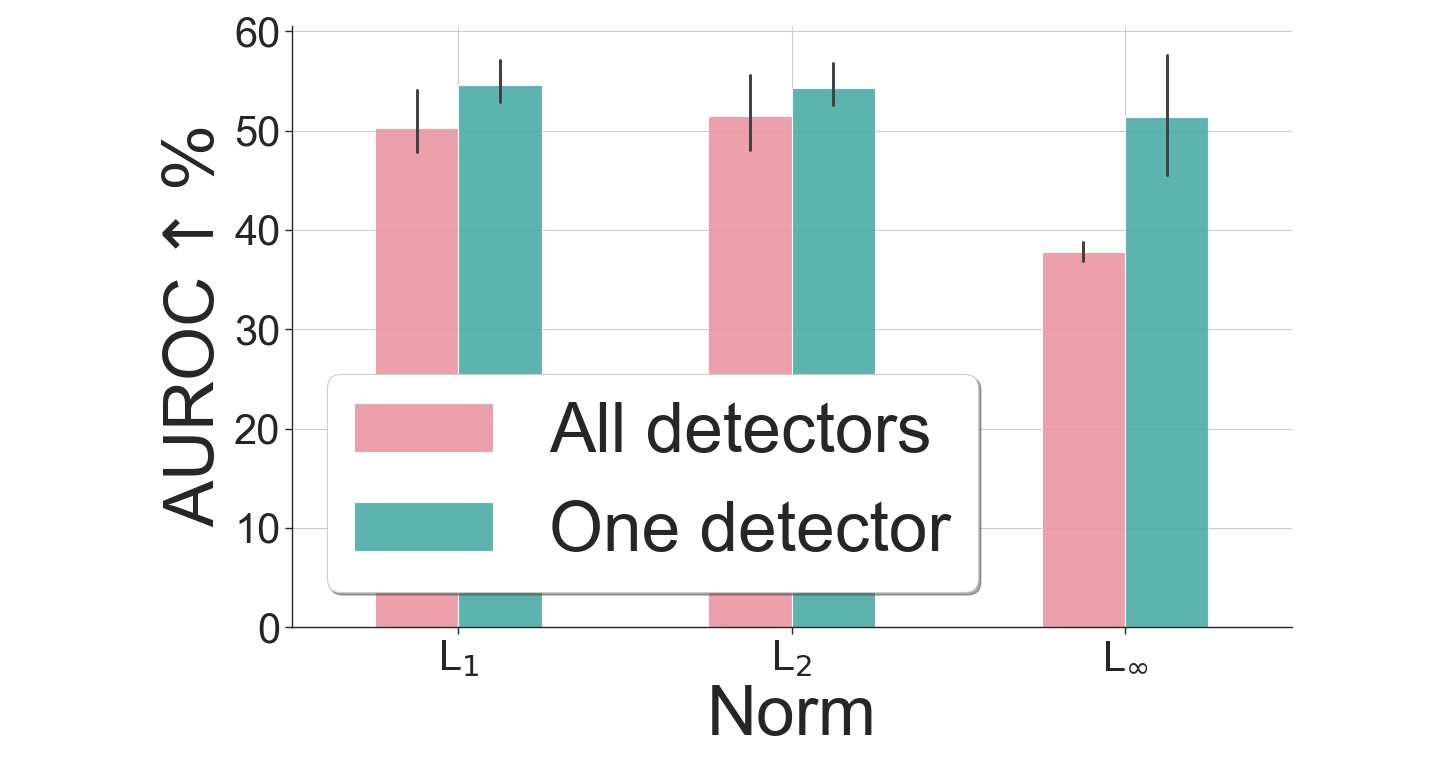
(a) Analysis AUROC$\uparrow$%

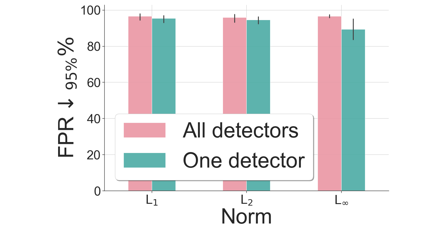
(b) Analysis FPR$\downarrow_{95\%}$%

Figure 8: Our method against the adaptive-attacks under Mead. We consider the worst case scenario in Tabs. 20 and 20, i.e., when $\alpha=0.1$.

We present a new experimental setting to address the case in which also the detectors are attacked at the same time as the target classifier, taking the cue from [Bryniarski et al., 2021, Carlini and Wagner, 2017a, Tramèr et al., 2020, Carlini and Wagner, 2017b]. It is important to note that, in the spirit of the Mead framework, we are not simply considering a scenario in which a single adaptive attack is perpetrated on the classifier and detectors, but rather multiple adaptive attacks are concurrently occurring. This scenario has not yet been considered in [Granese et al., 2022], so we are the first to deal with such a setting. We extend the framework to include two main cases: (i) for attacks on the classifier and the single detectors individually; (ii) for attacks on the classifier and all the detectors simultaneously.

The tables with the complete results are Tabs. 20 and 21, where $\alpha$ is the coefficient that controls the gradient’s speed of the attack against the detectors. We try many different values $\alpha=\left\{.1,1,5,10\right\}$. The case where $\alpha$ is equal to 0 is added for completeness, and it corresponds to the case where only the target classifier is attacked. We report in Fig. 8 the comparison of the results between case (i) and case (ii) on CIFAR10 and $\alpha=0.1$, as this corresponds to the case with the worst performances. As can be seen, the performances of our aggregator improve when the detectors are attacked singularly. This is particularly interesting for the setting we are dealing with. Indeed, our method is not a new supervised adversarial detection method but a framework to aggregate detectors, in this case, applied to the adversarial detection problem. Hence, it does not propose solving the problem of finding a new robust method for adaptive attacks but rather creating a mixture of experts based on the proposed sound mathematical framework. Thus, an attacker to successfully fool our method needs to have the complete access to all the underlying detectors and also an up-to-the-date knowledge of the detectors employed as the defender can always include a new detection mechanism to the pool of the detectors.

To give more insights on the proposed aggregator under this setting, we train a stronger version of the four shallow detectors where the detectors at training time have seen the corresponding adaptive attacks generated through the PGD algorithm. We report the results in Tab. 22 where we focus on the group of simultaneous attacks with L_∞ norm and $\varepsilon=0.25$ as this represents the worst result of our method in Tab. 21. If our method was only good as the best among the detectors, we should expect similar results in Tab. 22. In this case, the only solution would be to train a better detector. However, the strength of the aggregator is not just mimicking the performance of its parts but rather creating a mixture of experts based on the proposed sound mathematical framework. Therefore, we should expect better performances. Indeed, this consistently holds as the method performs much better than the best detector.

Table 22: Comparison between the proposed method and the single detectors (stronger version) against the adaptive-attacks. Norm L_∞ and $\varepsilon=0.25$ (i.e., attacks PGDi^⋆, FGSM^⋆, BIM^⋆).

CIFAR10	Ours	ACE	KL	FR	Gini
AUROC$\uparrow$%	54.6	35.7	30.6	26.3	36.2
FPR$\downarrow_{95\%}$%	73.0	96.5	97.0	97.4	99.6

B.10 AutoAttack [Croce and Hein, 2020] in the Proposed Solution

We present an application of AutoAttack [Croce and Hein, 2020], a state-of-the-art evaluation tool for robustness, redesigned for adversarial detection evaluation and adapted to our simultaneous attacks framework. In its original version, AutoAttack evaluates the accuracy of robust classifiers. In so doing,  [Croce and Hein, 2020] proposes a multiple attacks framework to ensure that at least one attack succeeds in producing an adversarial example for each natural one. In their context, it does not matter which attack will succeed since any successful attack would undermine the accuracy of the target classifier in the same way. In our case, the number of different successful attacks for each natural sample will affect the detection quality since a detector is successful only if it can detect all of them. Because of the above-mentioned differences, it is impossible to deploy it directly in our framework without any modifications. A modified version of AutoAttack adapted to the evaluation of our proposed method, has been implemented, and the results are presented below. While AutoAttack suggests using different attack strategies, in our case, we combine different attack strategies matched with different losses to make the pool of attacks more strong and more diversified.

Table 23: The proposed method on AutoAttack (Mead setting). The attacks are APGD-CE, APGD-DLR, FAB, SA.

	CIFAR10
	Ours
	AUROC$\uparrow$%	FPR$\downarrow_{95\%}$%
Norm L1
$\varepsilon=5$	57.1	88.4
$\varepsilon=10$	67.1	75.7
$\varepsilon=15$	72.2	66.7
$\varepsilon=20$	72.7	65.2
$\varepsilon=25$	72.8	65.6
$\varepsilon=30$	73.4	64.0
$\varepsilon=40$	73.6	64.0
Norm L2
$\varepsilon=0.125$	67.4	81.0
$\varepsilon=0.25$	58.0	89.0
$\varepsilon=0.3125$	58.1	88.8
$\varepsilon=0.5$	69.4	74.7
$\varepsilon=1$	75.1	61.6
$\varepsilon=1.5$	76.1	60.7
$\varepsilon=2$	76.1	60.5
Norm L∞
$\varepsilon=0.03125$	75.7	61.0
$\varepsilon=0.0625$	76.0	60.7
$\varepsilon=0.125$	76.8	60.3
$\varepsilon=0.25$	76.8	60.0
$\varepsilon=0.3125$	78.6	57.6
$\varepsilon=0.5$	76.1	60.3

References

- [Abdelnabi and Fritz, 2021] Abdelnabi, S. and Fritz, M. (2021). What’s in the box: Deflecting adversarial attacks by randomly deploying adversarially-disjoint models. In Jaeger, T. and Qian, Z., editors, MTD@CCS 2021: Proceedings of the 8th ACM Workshop on Moving Target Defense, Virtual Event, Republic of Korea, 15 November 2021, pages 3–12. ACM.
- [Aldahdooh et al., 2022] Aldahdooh, A., Hamidouche, W., Fezza, S. A., and Deforges, O. (2022). Adversarial example detection for dnn models: A review and experimental comparison. Artificial Intelligence Review.
- [Andriushchenko et al., 2020] Andriushchenko, M., Croce, F., Flammarion, N., and Hein, M. (2020). Square attack: A query-efficient black-box adversarial attack via random search. In Vedaldi, A., Bischof, H., Brox, T., and Frahm, J., editors, Computer Vision - ECCV 2020 - 16th European Conference, Glasgow, UK, August 23-28, 2020, Proceedings, Part XXIII, volume 12368 of Lecture Notes in Computer Science, pages 484–501. Springer.
- [Arimoto, 1972] Arimoto, S. (1972). An algorithm for computing the capacity of arbitrary discrete memoryless channels. IEEE Trans. Inf. Theory, 18(1):14–20.
- [Barron et al., 1998] Barron, A. R., Rissanen, J., and Yu, B. (1998). The minimum description length principle in coding and modeling. IEEE Trans. Inf. Theory, 44(6):2743–2760.
- [Ben-David et al., 2010] Ben-David, S., Blitzer, J., Crammer, K., Kulesza, A., Pereira, F., and Vaughan, J. W. (2010). A theory of learning from different domains. Mach. Learn., 79(1-2):151–175.
- [Bryniarski et al., 2021] Bryniarski, O., Hingun, N., Pachuca, P., Wang, V., and Carlini, N. (2021). Evading adversarial example detection defenses with orthogonal projected gradient descent. CoRR, abs/2106.15023.
- [Carlini et al., 2023] Carlini, N., Tramèr, F., Dvijotham, K. D., Rice, L., Sun, M., and Kolter, J. Z. (2023). (certified!!) adversarial robustness for free! In The Eleventh International Conference on Learning Representations, ICLR 2023, Kigali, Rwanda, May 1-5, 2023. OpenReview.net.
- [Carlini and Wagner, 2017a] Carlini, N. and Wagner, D. A. (2017a). Adversarial examples are not easily detected: Bypassing ten detection methods. In Thuraisingham, B., Biggio, B., Freeman, D. M., Miller, B., and Sinha, A., editors, Proceedings of the 10th ACM Workshop on Artificial Intelligence and Security, AISec@CCS 2017, Dallas, TX, USA, November 3, 2017, pages 3–14. ACM.
- [Carlini and Wagner, 2017b] Carlini, N. and Wagner, D. A. (2017b). Magnet and "efficient defenses against adversarial attacks" are not robust to adversarial examples. CoRR, abs/1711.08478.
- [Carlini and Wagner, 2017c] Carlini, N. and Wagner, D. A. (2017c). Towards evaluating the robustness of neural networks. In 2017 IEEE Symposium on Security and Privacy, SP 2017, San Jose, CA, USA, May 22-26, 2017, pages 39–57. IEEE Computer Society.
- [Chen et al., 2020] Chen, J., Jordan, M. I., and Wainwright, M. J. (2020). Hopskipjumpattack: A query-efficient decision-based attack. In 2020 IEEE Symposium on Security and Privacy, SP 2020, San Francisco, CA, USA, May 18-21, 2020, pages 1277–1294. IEEE.
- [Cohen et al., 2019] Cohen, J. M., Rosenfeld, E., and Kolter, J. Z. (2019). Certified adversarial robustness via randomized smoothing. In Chaudhuri, K. and Salakhutdinov, R., editors, Proceedings of the 36th International Conference on Machine Learning, ICML 2019, 9-15 June 2019, Long Beach, California, USA, volume 97 of Proceedings of Machine Learning Research, pages 1310–1320. PMLR.
- [Croce and Hein, 2020] Croce, F. and Hein, M. (2020). Reliable evaluation of adversarial robustness with an ensemble of diverse parameter-free attacks. In Proceedings of the 37th International Conference on Machine Learning, ICML 2020, 13-18 July 2020, Virtual Event, volume 119 of Proceedings of Machine Learning Research, pages 2206–2216. PMLR.
- [Davis and Goadrich, 2006] Davis, J. and Goadrich, M. (2006). The relationship between precision-recall and roc curves. In Proceedings of the 23rd international conference on Machine learning, pages 233–240.
- [Delattre et al., 2023] Delattre, B., Araujo, A., Barthélemy, Q., and Allauzen, A. (2023). The lipschitz-variance-margin tradeoff for enhanced randomized smoothing.
- [Engstrom et al., 2019] Engstrom, L., Tran, B., Tsipras, D., Schmidt, L., and Madry, A. (2019). Exploring the landscape of spatial robustness. In Chaudhuri, K. and Salakhutdinov, R., editors, Proceedings of the 36th International Conference on Machine Learning, ICML 2019, 9-15 June 2019, Long Beach, California, USA, volume 97 of Proceedings of Machine Learning Research, pages 1802–1811. PMLR.
- [Goodfellow et al., 2014] Goodfellow, I. J., Shlens, J., and Szegedy, C. (2014). Explaining and harnessing adversarial examples. arXiv preprint arXiv:1412.6572.
- [Goodfellow et al., 2015] Goodfellow, I. J., Shlens, J., and Szegedy, C. (2015). Explaining and harnessing adversarial examples. In Bengio, Y. and LeCun, Y., editors, 3rd International Conference on Learning Representations, ICLR 2015, San Diego, CA, USA, May 7-9, 2015, Conference Track Proceedings.
- [Granese et al., 2022] Granese, F., Picot, M., Romanelli, M., Messina, F., and Piantanida, P. (2022). MEAD: A multi-armed approach for evaluation of adversarial examples detectors. In European Conference on Machine Learning and Principles and Practice of Knowledge Discovery in Databases (ECML PKDD 2022), Grenoble, France, September 23, 2022.
- [Granese et al., 2021] Granese, F., Romanelli, M., Gorla, D., Palamidessi, C., and Piantanida, P. (2021). DOCTOR: A simple method for detecting misclassification errors. In Ranzato, M., Beygelzimer, A., Dauphin, Y. N., Liang, P., and Vaughan, J. W., editors, Advances in Neural Information Processing Systems 34: Annual Conference on Neural Information Processing Systems 2021, NeurIPS 2021, December 6-14, 2021, virtual, pages 5669–5681.
- [Grover et al., 2014] Grover, K., Lim, A. S., and Yang, Q. (2014). Jamming and anti-jamming techniques in wireless networks: a survey. Int. J. Ad Hoc Ubiquitous Comput., 17(4):197–215.
- [Kang et al., 2019] Kang, D., Sun, Y., Hendrycks, D., Brown, T., and Steinhardt, J. (2019). Testing robustness against unforeseen adversaries. arXiv preprint arXiv:1908.08016.
- [Karlof and Wagner, 2003] Karlof, C. and Wagner, D. (2003). Secure routing in wireless sensor networks: attacks and countermeasures. In Proceedings of the First IEEE International Workshop on Sensor Network Protocols and Applications, 2003., pages 113–127.
- [Kherchouche et al., 2020] Kherchouche, A., Fezza, S. A., Hamidouche, W., and Déforges, O. (2020). Detection of adversarial examples in deep neural networks with natural scene statistics. In 2020 International Joint Conference on Neural Networks, IJCNN 2020, Glasgow, United Kingdom, July 19-24, 2020, pages 1–7. IEEE.
- [Krizhevsky, 2009] Krizhevsky, A. (2009). Learning multiple layers of features from tiny images. Technical report.
- [Kurakin et al., ] Kurakin, A., Goodfellow, I. J., and Bengio, S. Adversarial examples in the physical world. In 5th International Conference on Learning Representations, ICLR 2017, Toulon, France, April 24-26, 2017, Workshop Track Proceedings.
- [Levine and Feizi, 2021] Levine, A. and Feizi, S. (2021). Improved, deterministic smoothing for l certified robustness. In Meila, M. and Zhang, T., editors, Proceedings of the 38th International Conference on Machine Learning, ICML 2021, 18-24 July 2021, Virtual Event, volume 139 of Proceedings of Machine Learning Research, pages 6254–6264. PMLR.
- [Madry et al., 2018] Madry, A., Makelov, A., Schmidt, L., Tsipras, D., and Vladu, A. (2018). Towards deep learning models resistant to adversarial attacks. In 6th International Conference on Learning Representations, ICLR 2018, Vancouver, BC, Canada, April 30 - May 3, 2018, Conference Track Proceedings.
- [Moosavi-Dezfooli et al., 2016] Moosavi-Dezfooli, S., Fawzi, A., and Frossard, P. (2016). Deepfool: A simple and accurate method to fool deep neural networks. In 2016 IEEE Conference on Computer Vision and Pattern Recognition, CVPR 2016, Las Vegas, NV, USA, June 27-30, 2016, pages 2574–2582. IEEE Computer Society.
- [Nandi et al., 2023] Nandi, S., Addepalli, S., Rangwani, H., and Babu, R. V. (2023). Certified adversarial robustness within multiple perturbation bounds. In IEEE/CVF Conference on Computer Vision and Pattern Recognition, CVPR 2023 - Workshops, Vancouver, BC, Canada, June 17-24, 2023, pages 2298–2305. IEEE.
- [Netzer et al., 2011] Netzer, Y., Wang, T., Coates, A., Bissacco, A., Wu, B., and Ng, A. Y. (2011). Reading digits in natural images with unsupervised feature learning. In NIPS Workshop on Deep Learning and Unsupervised Feature Learning 2011.
- [Pal et al., 2023] Pal, A., Sulam, J., and Vidal, R. (2023). Adversarial examples might be avoidable: The role of data concentration in adversarial robustness.
- [Pal and Vidal, 2020] Pal, A. and Vidal, R. (2020). A game theoretic analysis of additive adversarial attacks and defenses. In Larochelle, H., Ranzato, M., Hadsell, R., Balcan, M., and Lin, H., editors, Advances in Neural Information Processing Systems 33: Annual Conference on Neural Information Processing Systems 2020, NeurIPS 2020, December 6-12, 2020, virtual.
- [Pang et al., 2022] Pang, T., Zhang, H., He, D., Dong, Y., Su, H., Chen, W., Zhu, J., and Liu, T. (2022). Two coupled rejection metrics can tell adversarial examples apart. In IEEE/CVF Conference on Computer Vision and Pattern Recognition, CVPR 2022, New Orleans, LA, USA, June 18-24, 2022, pages 15202–15212. IEEE.
- [Perrig et al., 2004] Perrig, A., Stankovic, J., and Wagner, D. (2004). Security in wireless sensor networks. Communications of the ACM, 47(6):53–57.
- [Picot et al., 2022] Picot, M., Messina, F., Boudiaf, M., Labeau, F., Ayed, I. B., and Piantanida, P. (2022). Adversarial robustness via fisher-rao regularization. IEEE Transactions on Pattern Analysis & Machine Intelligence.
- [Raghunathan et al., 2018] Raghunathan, A., Steinhardt, J., and Liang, P. (2018). Certified defenses against adversarial examples. In 6th International Conference on Learning Representations, ICLR 2018, Vancouver, BC, Canada, April 30 - May 3, 2018, Conference Track Proceedings. OpenReview.net.
- [Raghuram et al., 2021] Raghuram, J., Chandrasekaran, V., Jha, S., and Banerjee, S. (2021). A general framework for detecting anomalous inputs to DNN classifiers. In Meila, M. and Zhang, T., editors, Proceedings of the 38th International Conference on Machine Learning, ICML 2021, 18-24 July 2021, Virtual Event, volume 139 of Proceedings of Machine Learning Research, pages 8764–8775. PMLR.
- [Sadeghi and Larsson, 2019] Sadeghi, M. and Larsson, E. G. (2019). Adversarial attacks on deep-learning based radio signal classification. IEEE Wireless Communications Letters, 8(1):213–216.
- [Slivkins et al., 2019] Slivkins, A. et al. (2019). Introduction to multi-armed bandits. Foundations and Trends® in Machine Learning, 12(1-2):1–286.
- [Szegedy et al., 2014] Szegedy, C., Zaremba, W., Sutskever, I., Bruna, J., Erhan, D., Goodfellow, I. J., and Fergus, R. (2014). Intriguing properties of neural networks. In Bengio, Y. and LeCun, Y., editors, 2nd International Conference on Learning Representations, ICLR 2014, Banff, AB, Canada, April 14-16, 2014, Conference Track Proceedings.
- [Tian et al., 2022] Tian, Q., Zhang, S., Mao, S., and Lin, Y. (2022). Adversarial attacks and defenses for digital communication signals identification. Digital Communications and Networks.
- [Tramèr et al., 2020] Tramèr, F., Carlini, N., Brendel, W., and Madry, A. (2020). On adaptive attacks to adversarial example defenses. In Larochelle, H., Ranzato, M., Hadsell, R., Balcan, M., and Lin, H., editors, Advances in Neural Information Processing Systems 33: Annual Conference on Neural Information Processing Systems 2020, NeurIPS 2020, December 6-12, 2020, virtual.
- [Vaishnavi et al., 2022] Vaishnavi, P., Eykholt, K., and Rahmati, A. (2022). Accelerating certified robustness training via knowledge transfer. In NeurIPS.
- [von Neumann, 1928] von Neumann, J. (1928). Zur theorie der gesellschaftsspiele. Mathematische Annalen, 100:295–320.
- [Xu et al., 2018] Xu, W., Evans, D., and Qi, Y. (2018). Feature squeezing: Detecting adversarial examples in deep neural networks. In 25th Annual Network and Distributed System Security Symposium, NDSS 2018, San Diego, California, USA, February 18-21, 2018. The Internet Society.
- [Zimmermann et al., 2022] Zimmermann, R. S., Brendel, W., Tramèr, F., and Carlini, N. (2022). Increasing confidence in adversarial robustness evaluations. CoRR, abs/2206.13991.