Neural optimal controller for stochastic systems via pathwise HJB operator

Abstract

The aim of this work is to develop deep learning-based algorithms for high-dimensional stochastic control problems based on physics-informed learning and dynamic programming. Unlike classical deep learning-based methods relying on a probabilistic representation of the solution to the Hamilton–Jacobi–Bellman (HJB) equation, we introduce a pathwise operator associated with the HJB equation so that we can define a problem of physics-informed learning. According to whether the optimal control has an explicit representation, two numerical methods are proposed to solve the physics-informed learning problem. We provide an error analysis on how the truncation, approximation and optimization errors affect the accuracy of these methods. Numerical results on various applications are presented to illustrate the performance of the proposed algorithms.

1 Itroduction

The range of stochastic optimal control (SOC) problems covers a variety of scientific branches such as movement neuroscience [1, 2] and robotics [3]. For solving the optimal control of stochastic systems, there are two powerful tools: Pontryagin’s maximum principle [4, 5, 6] and Bellman’s dynamic programming [7]. Based on these two tools, there are many numerical methods to solve the SOC problems.

• Pontryagin’s maximum principle (MP) gives a set of necessary conditions to obtain the optimal control, which can be written as extended stochastic Hamiltonian systems. The systems are forward-backward stochastic differential equations (SDEs), plus a maximum condition of a function called the Hamiltonian. The readers can refer to [8, 9, 10] and references therein in which the authors present some numerical methods for the forward-backward SDEs.

• Bellman’s dynamic programming (DP) reformulates the SOC problem to the Hamilton–Jacobi–Bellman (HJB) equation which is a backward parabolic-type partial differential equation (PDE). Various numerical methods have been developed to solve this PDE, for instance, finite-difference approximation [11], max-plus method [12], stochastic differential dynamic programing [13], path-integral control [14] and linearly solvable optimal control [15, 16].

However, these traditional numerical methods mentioned above are overall less efficient when the state dimension is large [17]. Despite great progress in the numerical discretization of PDEs, mesh generation in high-dimensional problems remains complex [18]. Indeed, the size of the discretized problem increases exponentially with spatial dimensions, making a direct solution intractable for even moderately large problems [19]. This is the so-called curse of dimensionality.

In recent years, we have seen tremendous progress in applying neural networks to solve high-dimensional PDEs. Many PDE solvers based on deep neural networks have been proposed for high-dimensional PDEs. We list some mainstreams of deep-learning frameworks for the parabolic-type PDEs:

• Sampling-based approach relies on a probabilistic representation of the solution to the parabolic-type PDEs via (nonlinear) Feynman–Kac formula. The pioneering papers [20, 21] proposed a neural network called deep BSDE method to solve a class of parabolic-type PDEs. Many related methods with this idea have been developed in [22, 23, 24, 25]. A comprehensive literature review about this approach can be found in [26].

• Physics-informed learning is to minimize the residual of the PDE and (artificial) boundary conditions at randomly sampled collocation points, such as deep Galerkin method [27] and physics-informed neural networks [28]. [29] provided a review of the related literature on physics-informed neural networks.

• Operator learning is designed as a general deep learning framework to learn diverse continuous nonlinear operators. This is a new line of work proposed to learn mesh-free, infinite-dimensional operator with neural networks such as DeepOnet [30] and Fourier Neural operator [31].

The approaches above pose possible ways to solve the curse of dimensionality in the field of SOC. Based on one of two classical tools, MP and DP, the corresponding deep learning-based methods developed recently can be divided into two categories. (i) With the aid of Stochastic MP, [32] and [33] respectively studied the problem of mean field games and mean field control by deep learning method. Specifically, [32] considered a specific linear-quadratic model, and [33] investigated a control problem in which the diffusion term does not depend on the control variable. In [34], stochastic optimal open-loop control was solved via stochastic MP with feedforward neural networks. (ii) Combining with the DP, [35, 36] reformulated the SOC problem as Markov decision process which is solved by some deep learning-based algorithms. In [21, 26], the authors simulated the HJB equation by using the backward SDE representation with a fully connected (FC) feedforward neural network. [37] and [38] proposed a deep learning-based algorithm that leverages the second order forward-backward SDE representation along with a long-short term memory (LSTM) recurrent neural network to solve the HJB equation.

Note that comparing with the methods based on DP, the methods via MP require more concavity and convexity assumptions [34, 39]. Moreover, the methods by using the sampling-based approach are under a decomposability assumption [17]. These assumptions restrict the deep learning-based methods mentioned above for practical applications.

In this paper, we aim to solve the SOC problem via DP with physics-informed learning. Comparing with the MP-based method [34] and the sampling-based method [17], our method based on DP is valid without any extra assumptions. Moreover, our method implemented by the physics-informed neural network (PINN) can be trained effectively just using small data sets, in comparison to the deep 2FBSDEs method in [38]. Another advantage of our method is mesh-free. Up to our knowledge, it is the first time to apply the physics-informed learning method to solve the SOC problem. The detailed comparison of this work with other related studies is summarized in Table 1.

Papers	Theory	Reformulation of SOC	Networks	$\star$	error analysis
[21, 26]	DP	backward SDE	FC	no	no
[34]	MP	Hamiltonian system	FC	no	no
[35, 36]	DP	State-action value function	FC	no	no
[37, 38]	DP	forward-backward SDEs	LSTM	yes	no
This work	DP	pathwise HJB operator	PINN	no	yes

Table 1: Comparison of this paper to some related works. Here, $\star$ denotes whether the optimal controls have an explicit representation.

The main contributions of this paper are summarized as follows. (i) Motivated by the sampling-based method, we introduce a pathwise HJB operator in Theorem 3.1, which is the key point to define the physics-informed learning problem. (ii) We propose two physics-informed learning-based methods to solve the pathwise HJB equation in Sections 4.1 and 4.2. (iii) While deep-learning based methods currently lack the mature error analysis that has been established for traditional numerical methods, we give an error analysis on our algorithms in Theorem 5.1. (iv) From the empirical results, we find the performance of the proposed method conducted by the LSTM architecture is better than that based on FC. A comparison of training time is shown in Figure 10, where it is clear that for low-dimensional nonlinear cases the LSTM network saves at least $40\%$ of training time than the FC network. For high-dimensional cases, we can see in Table 2 that the LSTM network can work well, while the FC network is invalid.

The remaining part of this paper is organized as follows. In Section 2, we briefly introduce the preliminaries about the SOC problem. For any partition of the time interval, we reformulate the corresponding HJB equation as a discrete scheme with a pathwise HJB operator in Section 3. We propose our numerical methods for solving the SOC problem and also give an error analysis on these algorithms in Section 4. Numerical examples in Section 6 illustrate our proposed methods. Section 7 provides some conclusions.

2 Problem statement

Let $T>t_{0}\geqslant 0$ and $\textbf{W}:[t_{0},T]\times\Omega\rightarrow\mathbb{R}^{\hat{d}}$ be a $\hat{d}$-dimensional standard $\mathbb{F}$-Brownian motions on a filtered probability space $(\Omega,\mathcal{F},\mathbb{F},\mathbb{P})$ where $\mathbb{F}=\{\mathcal{F}_{t}\}_{t_{0}\leqslant t\leqslant T}$ is the natural filtration generated by W. The quadruple $(\Omega,\mathcal{F},\mathbb{F},\mathbb{P})$ also satisfies the usual hypotheses. $\mathbb{E}[\cdot]$ stands for expectation with respect to the probability measure $\mathbb{P}$.

In this paper, we consider the following controlled stochastic differential equation

$$\mathrm{d}\textbf{x}_{t}=b(t,\textbf{x}_{t},\textbf{u}(t))\mathrm{d}t+\sigma(t,\textbf{x}_{t},\textbf{u}(t))\mathrm{d}\textbf{W}_{t}$$ (1)

with $t\in[t_{0},T]$ and the initial data $\textbf{x}_{t_{0}}=\textbf{x}\in\mathbb{R}^{n}$. Here, $\textbf{x}_{t}\in\mathbb{R}^{n}$ is the state process, $\textbf{u}(t)\in\mathbb{R}^{m}$ is a control process valued in a given subset $U$ of $\mathbb{R}^{m}$. The drift term $b$ and the diffusion term $\sigma$ are multivariable functions

$$b:[t_{0},T]\times\mathbb{R}^{n}\times\mathbb{R}^{m}\rightarrow\mathbb{R}^{n},\quad\sigma:[t_{0},T]\times\mathbb{R}^{n}\times\mathbb{R}^{m}\rightarrow\mathbb{R}^{n\times\hat{d}}.$$

The cost functional is given by

$$C(t_{0},\textbf{x};\textbf{u}(t))=\mathbb{E}\left[\int_{t_{0}}^{T}\phi(t,\textbf{x}_{t},\textbf{u}(t))\mathrm{d}t+\psi(\textbf{x}_{T})|\textbf{x}_{t_{0}}=\textbf{x}\right]$$ (2)

with the functions

$$\phi:[t_{0},T]\times\mathbb{R}^{n}\times\mathbb{R}^{m}\rightarrow\mathbb{R},\quad\psi:\mathbb{R}^{n}\rightarrow\mathbb{R}.$$

The goal of our SOC problem is to look for an admissible control (if exists) that minimizes (2) over $\mathcal{U}$ which is the set of all admissible controls defined by

$$\mathcal{U}:=\left\{u:[t_{0},T]\times\Omega\rightarrow U|u\in L^{2}_{\mathbb{F}}(t_{0},T;\mathbb{R}^{m})\right\}$$

in which $L^{2}_{\mathbb{F}}(t_{0},T;\mathbb{R}^{m})$ consists of all $\mathbb{F}$-adapted functions $u:[t_{0},T]\times\Omega\rightarrow\mathbb{R}^{m}$ satisfying $\mathbb{E}[\int_{t_{0}}^{T}|u|^{2}\mathrm{d}t]<\infty$. We call $\textbf{u}^{\ast}$ the optimal control which means

$$\textbf{u}^{\ast}:=\mathop{\arg\min}\limits_{\mathrm{u}\in\mathcal{U}}C(t_{0},\textbf{x},\textbf{u}^{\ast}).$$ (3)

The corresponding state process $\textbf{x}^{\ast}_{t}$ is called an optimal state process and the state-control pair $(\textbf{x}^{\ast}_{t},\textbf{u}^{\ast})$ called an optimal pair. Further, we define the value function as

$$q(t_{0},\textbf{x}):=C(t_{0},\textbf{x},\textbf{u}^{\ast})=\min\limits_{\mathrm{u}\in\mathcal{U}}C(t_{0},\textbf{x},\textbf{u}).$$ (4)

3 Pathwise HJB operator

Firstly let us make some standard assumptions [39, 40].

Assumption 1

The maps $b$, $\sigma$, $\phi$ and $\psi$ are all uniformly continuous satisfying

• there are constants $L_{1}>0$ and $L_{2}>0$ such that for $f=b$, $\sigma$, or $\phi$,

  $$|f(t,x_{1},u)-f(t,x_{2},u)|\leqslant L_{1}\{|x_{1}-x_{2}|\}$$

  and $|f(t,0,u)|\leqslant L_{2}$ for all $t\in[t_{0},T]$, $u\in\mathcal{U}$ and $x_{1},x_{2}\in\mathbb{R}^{n}$,

• $\psi$ is Lipschitz and $\psi(0)$ is bounded.

Assumption 2

The value function $q(t,x)$ belongs to $C^{1,2}([0,T]\times\mathbb{R}^{n})$, that is, once differentiable in $t$ and twice differentiable in $x\in\mathbb{R}^{n}$.

Under Assumptions 1 and 2, it deduces from the Proposition 3.5 of Chapter 4 in [39] that the value function $q(t,x)$ satisfies the following HJB equation

$$\left\{\begin{array}[]{ll}\partial_{t}q+H(t,x,\nabla q,\nabla^{2}q)=0,&t\in[0,T],\\ q(T,x)=\psi(x)\end{array}\right.$$ (5)

with the Hamiltonian function

$$H(t,x,\nabla q,\nabla^{2}q):=\min_{\mathrm{u}\in\mathcal{U}}\left[b\cdot\nabla q+\frac{1}{2}\mathrm{tr}\left(\nabla^{2}q\sigma\sigma^{\mathrm{T}}\right)+\phi\right].$$

Here, $\partial_{t}q$ means the first-order derivative of $q$ with respect to $t$, $\nabla q$ and $\nabla^{2}q$ respectively denote the gradient and the Hessian of $q(t,x)$ with respect to $x$, and $\mathrm{tr}$ is the abbreviation of the trace operator.

Since the HJB equation is a backward PDE defined in the whole spatial space, PINN cannot be applied to solve this PDE. Therefore, we need to introduce the pathwise HJB operator in the following theorem. It is derived from the stochastic verification theorem (see Chapter 5.5 in [39]) and gives the definition of the pathwise HJB operator.

Theorem 3.1

Let $q(t,x)$ be a solution of (5). Assume that $(t,x_{t})$ is an optimal path and $u(t)$ is the corresponding optimal control. Then, for any partition of the time interval $[0,T]:0=t_{0}<t_{1}<\cdots<t_{N}=T$, we have the discrete scheme

$$\left\{\begin{array}[]{ll}\mathcal{H}\left(q(t_{n},x_{t_{n}}),x_{t_{n}},u(t_{n})\right)=0,\\ q\left(t_{N},x_{t_{N}}\right)=\psi\left(x_{t_{N}}\right),\end{array}\right.$$

where the pathwised HJB operator $\mathcal{H}$ is given by

$$\mathcal{H}(q,x,u)=\partial_{t}q+b(t,x,u)\cdot\nabla q+\frac{1}{2}\mathrm{tr}\left[\nabla^{2}q(\sigma\sigma^{\mathrm{T}})(t,x,u)\right]+\phi(t,x,u).$$

Proof  Note that for any $t\in[0,T]$

$$q(t,x_{t})=C(t,x_{t},u(t))=\min\limits_{\mathrm{u}\in\mathcal{U}}C(t,x_{t},\mathrm{u})$$

satisfies the HJB equation (5). Based on the Theorem 5.1 in Chapter 5 of [39], we have

$$u(t)=\mathop{\arg\min}\limits_{\mathrm{u}\in\mathcal{U}}\left[b\cdot\nabla q+\frac{1}{2}\mathrm{tr}\left(\nabla^{2}q\sigma\sigma^{\mathrm{T}}\right)+\phi\right],$$

which implies the Hamiltonian function

$$H(t,x,\nabla q,\nabla^{2}q)=b(t,x,u(t))\cdot\nabla q(t,x)+\frac{1}{2}\mathrm{tr}\left[\nabla^{2}q(t,x)(\sigma\sigma^{\mathrm{T}})(t,x,u(t))\right]+\phi(t,x,u(t)).$$

Then, for any partition of the time interval $[0,T]$, we can obtain the discrete scheme and the pathwised HJB operator $\mathcal{H}$ stated in the theorem. $\square$

In the following, we consider a special case of SOC problems when the optimal control $\textbf{u}^{\ast}$ has an explicit expression. Many systems such as pendulum, cart-pole and quadcopter can reduce to this special case (see Appendix). These systems capture the essence of the control problem in robotics without covering all of the complexity that is often involved in real-world examples [3]. In more details, we consider the SOC problem under the following conditions.

• The drift term $b\in\mathbb{R}^{n}$ and the diffusion term $\sigma\in\mathbb{R}^{n\times(1+d)}$ in (1) have the following linear forms in control

  $$b(t,\textbf{x}_{t},\textbf{u}(t))=F(t,\textbf{x}_{t})+G(t,\textbf{x}_{t})\textbf{u}(t),\quad\sigma(t,\textbf{x}_{t},\textbf{u}(t))=[\lambda G(t,\textbf{x}_{t})\textbf{u}(t),H(t,\textbf{x}_{t})]$$

  with $\lambda\geqslant 0$, $F\in\mathbb{R}^{n}$, $G\in\mathbb{R}^{n\times m}$ and $H\in\mathbb{R}^{n\times d}$.

• The random term $\textbf{W}_{t}=[w^{(1)}_{t},w^{(2)}_{t}]\in\mathbb{R}^{(1+d)}$ in which $w^{(1)}_{t}\in\mathbb{R}^{1}$ and $w^{(2)}_{t}\in\mathbb{R}^{d}$ are mutually independent Brownian motions.

• The cost functional (2) is quadratic in control, that is,

  $$\phi(\textbf{x}_{t},\textbf{u}(t))=L(t,\textbf{x}_{t})+\frac{1}{2}\textbf{u}(t)^{\mathrm{T}}R\textbf{u}(t)$$

  with the control cost coefficient $R\in\mathbb{R}^{m\times m}$.

Thus, we have the following result which can be also seen in [38], but we calculate them anyway for the sake of completeness and to save the trouble of sending the reader to look at references.

Theorem 3.2

If (5) is solvable either analytically or numerically, then

$$\mathbf{u}^{\ast}(t)=-\tilde{R}^{-1}G^{\mathrm{T}}\nabla q$$ (6)

with $\tilde{R}=R+\lambda^{2}G^{\mathrm{T}}\nabla^{2}qG$. Moreover, the pathwised HJB operator in Theorem 3.1 can be reformulated as

$$\mathcal{H}(q,x_{t},u)$$

$$=\partial_{t}q+\frac{1}{2}\mathrm{tr}\left[\nabla^{2}q(HH^{\top})(t,x_{t})\right]+F(t,x_{t})\cdot\nabla q-\frac{1}{2}(\nabla q)^{\mathrm{T}}(G\tilde{R}^{-1}G^{\top})(q,x_{t},u)\nabla q+L(t,x_{t}).$$

Proof  Due to the specific expression of $b$, $\sigma$ and $\phi$, we observe that

$$\begin{aligned} H(t,x,\nabla q,\nabla^{2}q)=&\min_{\mathrm{u}}\left\{[G\textbf{u}(t)]\cdot\nabla q+\lambda^{2}\frac{1}{2}\textbf{u}(t)^{\mathrm{T}}G^{\mathrm{T}}\nabla^{2}qG\textbf{u}(t)+\frac{1}{2}\textbf{u}(t)^{\mathrm{T}}R\textbf{u}(t)\right\}\\ &+\frac{1}{2}\mathrm{tr}\left(\nabla^{2}qHH^{\mathrm{T}}\right)+f\cdot\nabla q+L.\end{aligned}$$ (7)

If (5) is solvable, then the optimal control is found by

$$\textbf{u}^{\ast}(t)=\mathop{\arg\min}\limits_{\mathrm{u}}\left[b\cdot\nabla q+\frac{1}{2}\mathrm{tr}\left(\nabla^{2}q\sigma\sigma^{\mathrm{T}}\right)+\phi\right].$$

Then by (7) the optimal control actually satisfies

$$\textbf{u}^{\ast}(t)=\mathop{\arg\min}\limits_{\mathrm{u}}\left\{[G\textbf{u}(t)]\cdot\nabla q+\lambda^{2}\frac{1}{2}\textbf{u}(t)^{\mathrm{T}}G^{\mathrm{T}}\nabla^{2}qG\textbf{u}(t)+\frac{1}{2}\textbf{u}(t)^{\mathrm{T}}R\textbf{u}(t)\right\}.$$

Since we have

$$\begin{aligned} \frac{\partial}{\partial u}\left\{[G\textbf{u}(t)]\cdot\nabla q+\lambda^{2}\frac{1}{2}\textbf{u}(t)^{\mathrm{T}}G^{\mathrm{T}}\nabla^{2}qG\textbf{u}(t)+\frac{1}{2}\textbf{u}(t)^{\mathrm{T}}R\textbf{u}(t)\right\}=0,\end{aligned}$$

that is,

$$\begin{aligned} G^{\mathrm{T}}\nabla q+\lambda^{2}G^{\mathrm{T}}\nabla^{2}qG\textbf{u}(t)+R\textbf{u}(t)=0\end{aligned}$$

then it deduces that

$$\textbf{u}^{\ast}(t)=-(R+\lambda^{2}G^{\mathrm{T}}\nabla^{2}qG)^{-1}G^{\mathrm{T}}\cdot\nabla q=-\tilde{R}^{-1}G^{\mathrm{T}}\nabla q$$

with $\tilde{R}=R+\lambda^{2}G^{\mathrm{T}}\nabla^{2}qG$.

Further, plugging the explicit expression of $\textbf{u}^{\ast}(t)$ into (7), the desired result follows immediately from the fact that

$$\begin{aligned} &\min_{\mathrm{u}}\left\{[G\textbf{u}(t)]\cdot\nabla q+\lambda^{2}\frac{1}{2}\textbf{u}(t)^{\mathrm{T}}G^{\mathrm{T}}\nabla^{2}qG\textbf{u}(t)+\frac{1}{2}\textbf{u}(t)^{\mathrm{T}}R\textbf{u}(t)\right\}\\ &=\left\{[G\textbf{u}(t)]\cdot\nabla q+\lambda^{2}\frac{1}{2}\textbf{u}(t)^{\mathrm{T}}G^{\mathrm{T}}\nabla^{2}qG\textbf{u}(t)+\frac{1}{2}\textbf{u}(t)^{\mathrm{T}}R\textbf{u}(t)\right\}\Big{|}_{\textbf{u}=\textbf{u}^{\ast}}\\ &=-(\nabla q)^{\mathrm{T}}G\tilde{R}^{-1}G\nabla q+\lambda^{2}\frac{1}{2}(\nabla q)^{\mathrm{T}}G\tilde{R}^{-\mathrm{T}}G^{\mathrm{T}}\nabla^{2}qG\tilde{R}^{-1}G^{\mathrm{T}}\nabla q+\frac{1}{2}(\nabla q)^{\mathrm{T}}G\tilde{R}^{-\mathrm{T}}R\tilde{R}^{-1}G^{\mathrm{T}}\nabla q\\ &=-(\nabla q)^{\mathrm{T}}G\tilde{R}^{-1}G\nabla q+\frac{1}{2}(\nabla q)^{\mathrm{T}}G\tilde{R}^{-\mathrm{T}}\tilde{R}\tilde{R}^{-1}G^{\mathrm{T}}\nabla q\\ &=-(\nabla q)^{\mathrm{T}}G\tilde{R}^{-1}G\nabla q+\frac{1}{2}(\nabla q)^{\mathrm{T}}G\tilde{R}^{-1}G^{\mathrm{T}}\nabla q\\ &=-\frac{1}{2}(\nabla q)^{\mathrm{T}}G\tilde{R}^{-1}G^{\mathrm{T}}\nabla q.\end{aligned}$$

Above all, we complete our proof. $\square$

4 Methodology

In this section we propose two novel numerical schemes to solve the HJB equation. Based on the pathwise HJB operator, we define the corresponding physics-informed learning problems which can be solved by a suitable variant of stochastic gradient descent (SGD).

Given the initial data $x_{0}$ and a partition of the time interval $[0,T]$:

$$0=t_{0}<t_{1}<\cdots<t_{n}<\cdots<t_{N}=T,$$

we consider the Euler–Maruyama scheme (cf. [41]) of (1)

$$x_{t_{n+1}}-x_{t_{n}}\approx b(t_{n},x_{t_{n}},u(t_{n}))\triangle t_{n}+\sigma(t_{n},x_{t_{n}},u(t_{n}))\triangle W_{n}$$ (8)

with $\triangle t_{n}=t_{n+1}-t_{n}$ and $\triangle W^{(i)}_{n}=W_{t_{n+1}}-W_{t_{n}}$. Using this scheme, the path $\{(t_{n},x_{t_{n}})\}_{0\leqslant n\leqslant N}$ can be easily generated. Then from Theorem 3.1 we have the temporal discretization of the pathwise HJB operator as follows.

$$\left\{\begin{array}[]{ll}\mathcal{H}\left(\{q(t_{n},x_{t_{n}}),x_{t_{n}},u(t_{n})\}_{0\leqslant n\leqslant N}\right)\approx 0,\\ q\left(t_{N},x_{t_{N}}\right)\approx\psi\left(x_{t_{N}}\right).\end{array}\right.$$ (9)

4.1 Numerical method with two neural networks

Note that in scheme (8) and (9) the control function $u$ and the value function $q$ are both unknown. Our key step is to simulating these two functions by two multilayer neural networks $q(t_{n},x_{t_{n}})\approx q^{\textrm{NN}}(t_{n},x_{t_{n}};\theta_{q})$ and $u(t_{n})\approx u^{\textrm{NN}}(t_{n},x_{t_{n}};\theta_{u})$, where $\{\theta_{q},\theta_{u}\}$ are the weights of the neural networks. Thereafter, (9) can be reformulated as

$$\left\{\begin{array}[]{ll}\mathcal{H}\left(\{q^{\textrm{NN}},x_{t_{n}},u^{\textrm{NN}}\}_{0\leqslant n\leqslant N}\right)\approx 0,\\ q^{\textrm{NN}}\left(t_{N},x_{t_{N}}\right)\approx\psi\left(x_{t_{N}}\right).\end{array}\right.$$ (10)

We now can define the physics-informed learning problem $\min_{\theta}L(\theta)$ where the loss function is given by

$$L(\theta_{q},\theta_{u})=\frac{1}{M}\sum\limits_{i=1}^{M}l_{i}(\theta_{q},\theta_{u})$$

with the number $M$ of samples and

$$\begin{split}l_{i}(\theta_{q},\theta_{u}):=\left|\mathcal{H}\left(q^{\textrm{NN}}(t_{n},x^{(i)}_{t_{n}};\theta_{q}),x^{(i)}_{t_{n}},u^{\textrm{NN}}(t_{n},x^{(i)}_{t_{n}};\theta_{u})\right)\right|^{2}+\left|q^{\textrm{NN}}(t_{N},x^{(i)}_{t_{N}};\theta_{q})-\psi(x^{(i)}_{t_{N}})\right|^{2}.\end{split}$$

We can now use a SGD-type algorithm to optimize the parameter $\{\theta_{q},\theta_{u}\}$. The pseudo-code for implementing this method is given in Algorithm 1. The neural networks we use here to approximate the control $u$ and the value function $q$ can be fully connected feedforward neural network or long-short term memory neural network. Figure 1 (a) illustrates the whole structure of physics-informed FC applied to solve the SOC problem, while Figure 1 (b) shows the whole architecture of physics-informed LSTM.

Algorithm 1 DeepHJB solver with 2-Net

0:  A partition of $[0,T]:0=t_{0}<t_{1}<\cdots<t_{N}=T$, initial data $\{(t_{0},x^{(i)}_{t_{0}})\}_{1\leqslant i\leqslant M}$, parameters $\theta^{(0)}$ of networks, learning rate $\eta$, max-step $K$

0:  $\{q(t_{n},x_{t_{n}})\}_{0\leqslant n\leqslant N}$, $\{u(t_{n})\}_{0\leqslant n\leqslant N}$

  for $k=0$ to $K-1$ do

     for $i\in B_{k}\subset[M]$ do

        for $n=0$ to $N$ do

           $q(t_{n},x^{(i)}_{t_{n}})\approx q^{\textrm{NN}}(t_{n},x^{(i)}_{t_{n}};\theta_{p}^{(k)})$

           $u^{(i)}(t_{n})\approx u^{\textrm{NN}}(t_{n},x^{(i)}_{t_{n}};\theta_{u}^{(k)})$

           while $n+1\leqslant N$ do

              $\triangle t_{n}=t_{n+1}-t_{n}$, $\triangle W^{(i)}_{n}=W^{(i)}_{t_{n+1}}-W^{(i)}_{t_{n}}$

              $x^{(i)}_{t_{n+1}}\approx x^{(i)}_{t_{n}}+b(t_{n},x^{(i)}_{t_{n}},u^{(i)}(t_{n}))\triangle t_{n}+\sigma(t_{n},x^{(i)}_{t_{n}},u^{(i)}(t_{n}))\triangle W^{(i)}_{n}$

           end while

        end for

     end for

     $\theta^{(k)}=(\theta_{p}^{(k)},\theta_{u}^{(k)})$

     $\mathrm{Loss}(\theta^{(k)})=\frac{1}{|B_{k}|}\sum\limits_{i\in B_{k}}l_{i}(\theta^{k})$

     $\theta^{(k+1)}=\theta^{(k)}-\eta\nabla\mathrm{Loss}(\theta^{(k)})$

  end for

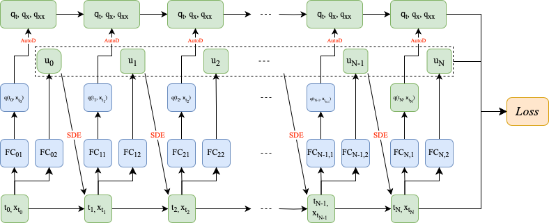
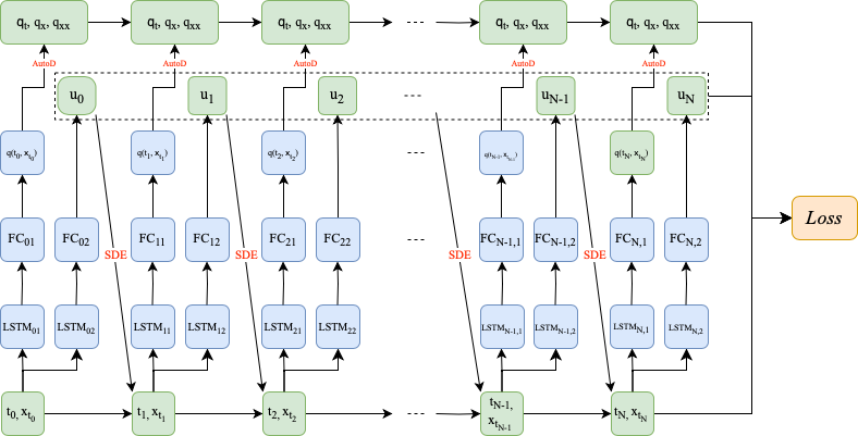
Figure 1: The whole network architectures of Algorithm 1: (a) PI-FC; (b) PI-LSTM. The data in the green boxes will used to calculate the loss. The solid lines represent the data flow generated in the current iteration. AutoD is short of the automatic differentiation. SDE means the Euler-Maruyama scheme.

4.2 Numerical method with one neural network

When the explicit formula of the control $u$ is available, from (6) we can calculate the approximation value of $u$ by

$$u(t_{n})\approx-\tilde{R}^{-1}(t_{n},x_{t_{n}})G^{\mathrm{T}}(t_{n},x_{t_{n}})\nabla q(t_{n},x_{t_{n}}).$$ (11)

If the value function $q(t_{n},x_{t_{n}})$ is approximated by a neural network $q^{\textrm{NN}}(t_{n},x_{t_{n}};\theta)$, then we obtain the simulation of $\nabla q(t_{n},x_{t_{n}})$, denoted by $\nabla q^{\textrm{NN}}(t_{n},x_{t_{n}};\theta)$, by using the automatic differentiation. Combining (11) gives

$$u(t_{n})\approx-\tilde{R}^{-1}(t_{n},x_{t_{n}})G^{\mathrm{T}}(t_{n},x_{t_{n}})\nabla q^{\textrm{NN}}(t_{n},x_{t_{n}};\theta).$$

Similarly, we can define the following physics-informed learning problem

$$\min_{\theta}L(\theta)=\min_{\theta}\left\{\frac{1}{M}\sum\limits_{i=1}^{M}l_{i}(\theta)\right\}$$

with

$$\begin{split}l_{i}(\theta):=\left|\mathcal{H}\left(q^{\textrm{NN}}(t_{n},x^{(i)}_{t_{n}};\theta),x^{(i)}_{t_{n}},u(t_{n},x^{(i)}_{t_{n}})\right)\right|^{2}+\left|q^{\textrm{NN}}(t_{N},x^{(i)}_{t_{N}};\theta)-\psi(x^{(i)}_{t_{N}})\right|^{2}.\end{split}$$

To solve this physics-informed learning problem, we can use a stochastic gradient descent-type method to optimize the parameter $\{\theta_{p}\}$. The pseudo-code is given as Algorithm 2. Figure 2 gives the whole network structures for all the time-points.

Algorithm 2 DeepHJB solver with 1-Net

0:  A partition of $[0,T]:0=t_{0}<t_{1}<\cdots<t_{N}=T$, initial data $\{(t_{0},x^{(i)}_{t_{0}})\}_{1\leqslant i\leqslant M}$, parameters $\theta^{(0)}$ of networks, learning rate $\eta$, max-step $K$

0:  $\{q(t_{n},x_{t_{n}})\}_{0\leqslant n\leqslant N}$, $\{u(t_{n})\}_{0\leqslant n\leqslant N}$

  for $k=0$ to $K-1$ do

     for $i\in B_{k}\subset[M]$ do

        for $n=0$ to $N$ do

           $q(t_{n},x^{(i)}_{t_{n}})\approx q^{\textrm{NN}}(t_{n},x^{(i)}_{t_{n}};\theta^{(k)})$

           $u^{(i)}(t_{n})\approx-\tilde{R}^{-1}(t_{n},x^{(i)}_{t_{n}})G^{\mathrm{T}}(t_{n},x^{(i)}_{t_{n}})\nabla q^{\textrm{NN}}(t_{n},x^{(i)}_{t_{n}};\theta^{(k)})$

           while $n+1\leqslant N$ do

              $\triangle t_{n}=t_{n+1}-t_{n}$, $\triangle W^{(i)}_{n}=W^{(i)}_{t_{n+1}}-W^{(i)}_{t_{n}}$

              $x^{(i)}_{t_{n+1}}\approx x^{(i)}_{t_{n}}+b(t_{n},x^{(i)}_{t_{n}},u^{(i)}(t_{n}))\triangle t_{n}+\sigma(t_{n},x^{(i)}_{t_{n}},u^{(i)}(t_{n}))\triangle W^{(i)}_{n}$

           end while

        end for

     end for

     $\mathrm{Loss}(\theta^{(k)})=\frac{1}{|B_{k}|}\sum\limits_{i\in B_{k}}l_{i}(\theta^{k})$

     $\theta^{(k+1)}=\theta^{(k)}-\eta\nabla\mathrm{Loss}(\theta^{(k)})$

  end for

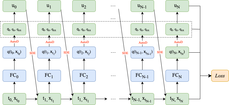
Figure 2: The whole network architectures of Algorithm 2: (a) PI-FC; (b) PI-LSTM. The data in the green boxes will used to calculate the loss. The solid lines represent the data flow generated in the current iteration. AutoD is short of the automatic differentiation. SDE means the Euler-Maruyama scheme.

5 Error analysis

As can be seen in Algorithm 1 and 2, there are three major sources of error, namely, truncation error of path generating, approximation error $\varepsilon^{\textrm{approx}}$ of neural network and optimization error $\varepsilon^{\textrm{opt}}$ of each iteration for solving the physics-informed learning problem. We give an analysis on how these three errors affect the accuracy of our numerical methods in the following theorem.

For better readability we suppress the superscript $(i)$ in the following theorem for error analysis and assume the time interval $[0,T]$ is partitioned evenly, that is, $\triangle t=t_{n+1}-t_{n}=\frac{T}{N}$ for $n=0,1,\cdots,N$, $N\geqslant 1$.

Theorem 5.1

Assume the physics-informed learning problems defined in Sections 4.1 and 4.2 can be solved by the proposed SGD-type algorithm. Let $q(t,x)$ be a solution of (5), $\hat{x}_{t}$ the exact path and $x_{t_{n}}$ the approximating path generated by (8). Then, there exist constants $C_{T}>0$, dependent on $T$, and $K_{0}>0$ such that for any $K\geqslant K_{0}$

$$\begin{split}\mathbb{E}|q(t_{n},\hat{x}_{t_{n}})-q^{\mathrm{NN}}(t_{n},x_{t_{n}};\theta^{(K)})|^{2}<C_{T}\left[(\varepsilon^{\mathrm{approx}}+\varepsilon^{\mathrm{opt}})^{2}+\triangle t\right].\end{split}$$

Proof  The subsequent proof consists of several steps.

Step 1. Note that the following estimation holds

$$\mathbb{E}|q(t_{n},\hat{x}_{t_{n}})-q^{\textrm{NN}}(t_{n},x_{t_{n}};\theta^{(K)}_{q})|^{2}\leqslant E_{1}+E_{2}$$ (12)

with

$$E_{1}=\mathbb{E}|q(t_{n},\hat{x}_{t_{n}})-q(t_{n},x_{t_{n}})|^{2}$$

and

$$E_{2}=\mathbb{E}|q(t_{n},x_{t_{n}})-q^{\textrm{NN}}(t_{n},x_{t_{n}};\theta^{(K)}_{q})|^{2}.$$

By the universal approximation theorem in [42], there exists a neural network denoted by $q^{\textrm{NN}}(t_{n},x_{t_{n}};\theta^{\ast}_{q})$ such that

$$|q(t_{n},x_{t_{n}})-q^{\textrm{NN}}(t_{n},x_{t_{n}};\theta_{q}^{\ast})|\leqslant\varepsilon^{\textrm{approx}}$$

with $n=0,1,\cdots,N$. Since the automatic differentiation itself does not incur truncation error, then we have

$$|\nabla q(t_{n},x_{t_{n}})-\nabla q^{\textrm{NN}}(t_{n},x_{t_{n}};\theta_{q}^{\ast})|<\varepsilon^{\textrm{approx}},\quad|\nabla^{2}q(t_{n},x_{t_{n}})-\nabla^{2}q^{\textrm{NN}}(t_{n},x_{t_{n}};\theta_{q}^{\ast})|<\varepsilon^{\textrm{approx}},$$ (13)

if $\nabla q$ and $\nabla^{2}q$ are computed from $q^{\textrm{NN}}$ via the automatic differentiation. Due to the physics-informed learning problem is assumed to be solvable, then there exists a constant $K_{0}>0$ such that for any $K\geqslant K_{0}$

$$|q^{\textrm{NN}}(t_{n},x_{t_{n}};\theta_{q}^{\ast})-q^{\textrm{NN}}(t_{n},x_{t_{n}};\theta^{(K)}_{q})|\leqslant\varepsilon^{\textrm{opt}}.$$

Similarly, we also have

$$\begin{split}&|\nabla q^{\textrm{NN}}(t_{n},x_{t_{n}};\theta^{(K)}_{q})-\nabla q^{\textrm{NN}}(t_{n},x_{t_{n}};\theta_{q}^{\ast})|<\varepsilon^{\textrm{opt}},\\ &|\nabla^{2}q^{\textrm{NN}}(t_{n},x_{t_{n}};\theta^{(K)}_{q})-\nabla^{2}q^{\textrm{NN}}(t_{n},x_{t_{n}};\theta_{q}^{\ast})|<\varepsilon^{\textrm{opt}}.\end{split}$$ (14)

We have the following observation

$$\begin{split}&|q(t_{n},x_{t_{n}})-q^{\textrm{NN}}(t_{n},x_{t_{n}};\theta^{(K)}_{q})|\\ &\leqslant|q(t_{n},x_{t_{n}})-q^{\textrm{NN}}(t_{n},x_{t_{n}};\theta_{q}^{\ast})|+|q^{\textrm{NN}}(t_{n},x_{t_{n}};\theta_{q}^{\ast})-q^{\textrm{NN}}(t_{n},x_{t_{n}};\theta^{(K)}_{q})|\end{split}$$

which implies $E_{2}<(\varepsilon^{\textrm{approx}}+\varepsilon^{\textrm{opt}})^{2}$. Then by (12), we obtain

$$\begin{aligned} &\mathbb{E}|q(t_{n},\hat{x}_{t_{n}})-q^{\textrm{NN}}(t_{n},x_{t_{n}};\theta^{(K)}_{q})|^{2}\\ &\leqslant\mathbb{E}|q(t_{n},\hat{x}_{t_{n}})-q(t_{n},x_{t_{n}})|^{2}+\mathbb{E}|q(t_{n},x_{t_{n}})-q^{\textrm{NN}}(t_{n},x_{t_{n}};\theta^{(K)}_{q})|^{2}\\ &\leqslant C\mathbb{E}|\hat{x}_{t_{n}}-x_{t_{n}}|^{2}+(\varepsilon^{\textrm{approx}}+\varepsilon^{\textrm{opt}})^{2},\end{aligned}$$ (15)

where the first term in the second inequality comes from the fact that $q$ is $C^{2}$ in space variable. Then we should complete our proof if we estimate the term $\mathbb{E}|\hat{x}_{t_{n}}-x_{t_{n}}|^{2}$ in (15).

Step 2. For $0\leqslant t\leqslant T$, let us define

$$\begin{aligned} Z(t)=\sup_{0\leqslant s\leqslant t}\mathbb{E}|\hat{x}_{s}-\tilde{x}_{s}|^{2},\end{aligned}$$

where the exact solution $\hat{x}_{s}$ satisfies

$$\hat{x}_{s}=x_{0}+\int_{0}^{s}b(\tau,\hat{x}_{\tau},\hat{u}(\tau))d\tau+\int_{0}^{s}\sigma(\tau,\hat{x}_{\tau},\hat{u}(\tau))dW_{\tau},$$

and the piecewise constant solution $\tilde{x}_{s}=x_{t_{n}}$, for $t_{n}\leqslant s<t_{{n}+1}$, satisfies

$$\tilde{x}_{s}=x_{0}+\int_{0}^{t_{n}}b(\tau,\tilde{x}_{\tau},u(\tau))d\tau+\int_{0}^{t_{n}}\sigma(\tau,\tilde{x}_{\tau},u(\tau))dW_{\tau}.$$

Then we have

$$\begin{aligned} Z(t)&=\sup_{0\leqslant s\leqslant t}\mathbb{E}\Big{[}\int_{0}^{t_{n}}|b(\tau,\hat{x}_{\tau},\hat{u}(\tau))-b(\tau,\tilde{x}_{\tau},u(\tau))|d\tau+\int_{0}^{t_{n}}|\sigma(\tau,\hat{x}_{\tau},\hat{u}(\tau))-\sigma(\tau,\tilde{x}_{\tau},u(\tau))|dW_{\tau}\\ &\qquad+\int_{t_{n}}^{s}b(\tau,\hat{x}_{\tau},\hat{u}(\tau))d\tau+\int_{t_{n}}^{s}\sigma(\tau,\hat{x}_{\tau},\hat{u}(\tau))dW_{\tau}\Big{]}^{2}\\ &\leqslant 4\sup_{0\leqslant s\leqslant t}\mathbb{E}\Big{[}|\int_{0}^{t_{n}}|b(\tau,\hat{x}_{\tau},\hat{u}(\tau))-b(\tau,\tilde{x}_{\tau},u(\tau))|d\tau|^{2}\\ &\qquad+|\int_{0}^{t_{n}}|\sigma(\tau,\hat{x}_{\tau},\hat{u}(\tau))-\sigma(\tau,\tilde{x}_{\tau},u(\tau))|dW_{\tau}|^{2}\\ &\qquad+|\int_{t_{n}}^{s}b(\tau,\hat{x}_{\tau},\hat{u}(\tau))d\tau|^{2}+|\int_{t_{n}}^{s}\sigma(\tau,\hat{x}_{\tau},\hat{u}(\tau))dW_{\tau}|^{2}\Big{]}.\end{aligned}$$

Using the linearity of the expectation, Cauchy–Schwarz’s inequality and Itô’s isometry, we obtain

$$\begin{aligned} Z(t)&\leqslant 4\sup_{0\leqslant s\leqslant t}\mathbb{E}\Big{[}|\int_{0}^{t_{n}}|b(\tau,\hat{x}_{\tau},\hat{u}(\tau))-b(\tau,\tilde{x}_{\tau},u(\tau))|d\tau|^{2}\\ &\qquad+|\int_{0}^{t_{n}}|\sigma(\tau,\hat{x}_{\tau},\hat{u}(\tau))-\sigma(\tau,\tilde{x}_{\tau},u(\tau))|dW_{\tau}|^{2}\\ &\qquad+|\int_{t_{n}}^{s}b(\tau,\hat{x}_{\tau},\hat{u}(\tau))d\tau|^{2}+|\int_{t_{n}}^{s}\sigma(\tau,\hat{x}_{\tau},\hat{u}(\tau))dW_{\tau}|^{2}\Big{]}\\ &\leqslant 4\sup_{0\leqslant s\leqslant t}\Big{(}T\mathbb{E}\left[\int_{0}^{t_{n}}|b(\tau,\hat{x}_{\tau},\hat{u}(\tau))-b(\tau,\tilde{x}_{\tau},u(\tau))|^{2}d\tau\right]\\ &\qquad+\mathbb{E}\left[\int_{0}^{t_{n}}|\sigma(\tau,\hat{x}_{\tau},\hat{u}(\tau))-\sigma(\tau,\tilde{x}_{\tau},u(\tau))|^{2}d\tau\right]\\ &\qquad+\triangle t\mathbb{E}\left[\int_{t_{n}}^{s}|b(\tau,\hat{x}_{\tau},\hat{u}(\tau))|^{2}d\tau\right]+\mathbb{E}\left[\int_{t_{n}}^{s}|\sigma(\tau,\hat{x}_{\tau},\hat{u}(\tau))|^{2}d\tau\right]\Big{)}.\end{aligned}$$

By Assumption 1 and the boundedness of $\sup\limits_{0\leqslant s\leqslant T}\mathbb{E}|\hat{x}_{s}|^{2}$, we have

$$\begin{aligned} Z(t)&\leqslant 4\sup_{0\leqslant s\leqslant t}\Big{(}L_{2}(T+1)\mathbb{E}\left[\int_{0}^{t_{n}}|\hat{x}_{\tau}-\tilde{x}_{\tau}|^{2}+|\hat{u}(\tau)-u(\tau)|^{2}d\tau\right]\\ &\qquad+L_{1}(\triangle t+1)\mathbb{E}\left[\int_{t_{n}}^{s}(1+|\hat{x}_{\tau}|)^{2}d\tau\right]\Big{)}\\ &\leqslant 4\sup_{0\leqslant s\leqslant t}\Big{(}L_{2}(T+1)\mathbb{E}\left[\int_{0}^{t_{n}}|\hat{x}_{\tau}-\tilde{x}_{\tau}|^{2}+|\hat{u}(\tau)-u(\tau)|^{2}d\tau\right]\Big{)}\\ &\qquad+L_{1}\triangle t(\triangle t+1)(1+\sup_{0\leqslant s\leqslant T}\mathbb{E}|\hat{x}_{s}|^{2})\\ &\leqslant 4\sup_{0\leqslant s\leqslant t}\Big{(}L_{2}(T+1)\mathbb{E}\left[\int_{0}^{t_{n}}|\hat{x}_{\tau}-\tilde{x}_{\tau}|^{2}+|\hat{u}(\tau)-u(\tau)|^{2}d\tau\right]\Big{)}+C_{T}\triangle t.\end{aligned}$$ (16)

Step 3. We have the following two cases with respect to the two types of network architecture.

• Case 1. If the control term $u(s)$ is also approximated by a neural network, then there exists a constant $K_{2}>0$ such that for any $K\geqslant K_{2}$

  $$\begin{aligned} |\hat{u}(s)-u^{\textrm{NN}}(s;\theta_{u}^{(K)})|<(\varepsilon^{\textrm{approx}}+\varepsilon^{\textrm{opt}})^{2}.\end{aligned}$$ (17)

From (16) it deduces that

$$\begin{aligned} Z(t)&\leqslant C_{T}\left(\int_{0}^{t}Z(\tau)d\tau+\sup_{0\leqslant s\leqslant T}\mathbb{E}|\hat{u}(s)-u(s)|^{2}+\triangle t\right).\end{aligned}$$ (18)

Combining (17) and (18) gives

$$\begin{aligned} Z(t)&\leqslant C_{T}\left(\int_{0}^{t}Z(\tau)d\tau+(\varepsilon^{\textrm{approx}}+\varepsilon^{\textrm{opt}})^{2}+\triangle t\right).\end{aligned}$$ (19)

By Gronwall’s inequality, it follows that

$$Z(T)=\sup_{0\leqslant s\leqslant T}\mathbb{E}|\hat{x}_{s}-\tilde{x}_{s}|^{2}\leqslant C_{T}\left[(\varepsilon^{\textrm{approx}}+\varepsilon^{\textrm{opt}})^{2}+\triangle t\right].$$ (20)

Due to (15) and (20), we obtain

$$\begin{aligned} \mathbb{E}|q(t_{n},\hat{x}_{t_{n}})-q^{\textrm{NN}}(t_{n},x_{t_{n}};\theta^{(K)}_{q})|^{2}\leqslant C_{T}\left[(\varepsilon^{\textrm{approx}}+\varepsilon^{\textrm{opt}})^{2}+\triangle t\right].\end{aligned}$$ (21)

• Case 2. If the control has an explicit expression (6), we have the estimate for the difference between the real control $\hat{u}(s)$ and the approximating control $u(s)$

  $$\begin{aligned} &|\hat{u}(s)-u(s)|\\ &\leqslant|-\tilde{R}^{-1}(s,\hat{x}_{s})G^{\mathrm{T}}(s,\hat{x}_{s})\nabla q(s,\hat{x}_{s})+\tilde{R}^{-1}(s,\tilde{x}_{s})G^{\mathrm{T}}(s,\tilde{x}_{s})\nabla q^{\textrm{NN}}(s,\tilde{x}_{s};\theta^{(K)})|\\ &\leqslant|\tilde{R}^{-1}(s,\hat{x}_{s})G^{\mathrm{T}}(s,\hat{x}_{s})\nabla q(s,\hat{x}_{s})-\tilde{R}^{-1}(s,\hat{x}_{s})G^{\mathrm{T}}(s,\hat{x}_{s})\nabla q(s,\tilde{x}_{s})|\\ &\quad+|\tilde{R}^{-1}(s,\hat{x}_{s})G^{\mathrm{T}}(s,\hat{x}_{s})\nabla q(s,\tilde{x}_{s})-\tilde{R}^{-1}(s,\tilde{x}_{s})G^{\mathrm{T}}(s,\tilde{x}_{s})\nabla q^{\textrm{NN}}(s,\tilde{x}_{s};\theta^{(K)})|\\ &\leqslant|\tilde{R}^{-1}(s,\hat{x}_{s})G^{\mathrm{T}}(s,\hat{x}_{s})||\nabla q(s,\hat{x}_{s})-\nabla q(s,\tilde{x}_{s})|\\ &\quad+|\tilde{R}^{-1}(s,\hat{x}_{s})G^{\mathrm{T}}(s,\hat{x}_{s})-\tilde{R}^{-1}(s,\tilde{x}_{s})G^{\mathrm{T}}(s,\tilde{x}_{s})||\nabla q(s,\tilde{x}_{s})|\\ &\quad+|\tilde{R}^{-1}(s,\tilde{x}_{s})G^{\mathrm{T}}(s,\tilde{x}_{s})||\nabla q(s,\tilde{x}_{s})-\nabla q^{\textrm{NN}}(s,\tilde{x}_{s};\theta^{(K)})|,\end{aligned}$$

  which implies

  $$\begin{aligned} |\hat{u}(s)-u(s)|&\leqslant C_{1}|\hat{x}_{s}-\tilde{x}_{s}|+C_{2}|\nabla q(s,\tilde{x}_{s})-\nabla q^{\textrm{NN}}(s,\tilde{x}_{s};\theta^{(K)})|\\ &\quad+C_{3}|\nabla^{2}q(s,\tilde{x}_{s})-\nabla^{2}q^{\textrm{NN}}(s,\tilde{x}_{s};\theta^{(K)})|.\end{aligned}$$ (22)

From (13), (14), (16) and (22) it implies that

$$\begin{aligned} Z(t)&\leqslant C_{T}\left(\int_{0}^{t}Z(\tau)d\tau+2(\varepsilon^{\textrm{approx}}+\varepsilon^{\textrm{opt}})^{2}+\triangle t\right).\end{aligned}$$

Similar as in case 1, we also obtain

$$\begin{aligned} \mathbb{E}|q(t_{n},\hat{x}_{t_{n}})-q^{\textrm{NN}}(t_{n},x_{t_{n}};\theta^{(K)}_{q})|^{2}\leqslant C_{T}\left[(\varepsilon^{\textrm{approx}}+\varepsilon^{\textrm{opt}})^{2}+\triangle t\right].\end{aligned}$$ (23)

Step 4. Let $K_{0}=\max\{K_{1},K_{2}\}$. Based on (21) and (23), this complete the proof. $\square$

Remark 5.1

The value of $\triangle t$ affect the truncation error. As $N$ increases, the value of $\triangle t$ will decrease. As a consequence, the total errors of Algorithms 1 and 2 become smaller and smaller.

6 Simulation

To evaluate the performance of our proposed algorithms, we apply them to solve some SOC problems. The tasks of these problems are to command the states of the motions moving from its initial point $\mathbf{x}_{0}$ to the target state $\mathbf{x}_{T}$ at time $T>0$. The cost functional in these problems is a quadratic functional of the form

$$J(u)=\mathbb{E}\left\{\int_{0}^{T}\left[x_{t}^{\top}Qx_{t}+\frac{1}{2}u_{t}^{\top}Ru_{t}\right]dt-x_{T}^{\top}Q_{T}x_{T}\right\}.$$ (24)

We gather the statistics (means and deviations) of numerical results from $30$ independent runs of each algorithm. In all plots, the solid lines represent mean trajectories and the shaded regions represent the $95\%$ confidence region (mean $\pm$ standard deviation). The learning rates varies to adjust to different examples.

6.1 Control without an explicit representation

Example 1. Consider the following controlled SDE (cf. example 4.2.4 in [34])

$$dx_{t}=\sin u_{t}dt+x_{t}dW_{t},\quad t\in[0,T]$$

with the cost functional (24). It is clear that the optimal control in this problem does not have an explicit representation. Then we can use the DeepHJB solver with 2-Net (Algorithm 1) conducted by LSTM and FC to solve this control problem. The parameters for simulation are given as follows.

$T$	$N$	$M$	$Q$	$Q_{T}$	$R$	$\mathbf{x}_{0}$	$\mathbf{x}_{T}$
$3.0$	$50$	$50$	$4$	$100$	$2.0$	$1.0$	$0$

The left of Figure 3 illustrates the state trajectories across all time steps. It can be observed that the task of SOC problem is completed with low variance. The middle of Figure 3 shows the corresponding neural optimal controller, and the time evolution of the value function is given in the right of Figure 3.

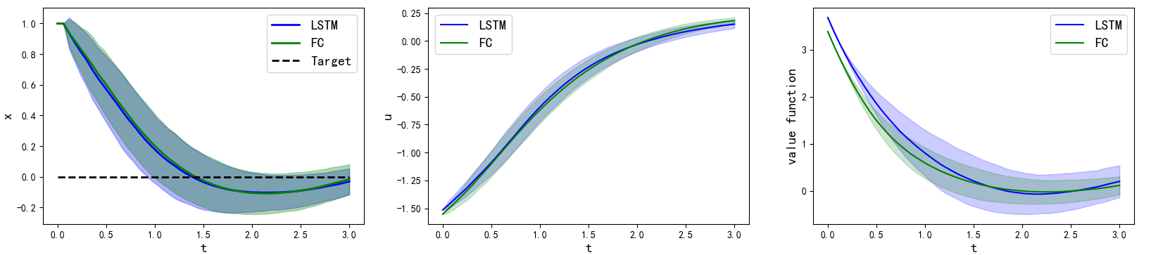
Figure 3: Numerical results of Example 1. Left: state trajectory; Middle: neural optimal controller; Right: the value function.

6.2 Linear control problems

Example 2. Consider the controlled multi-agent system

$$dx_{t}=\left(Ax_{t}+Gu_{t}\right)dt+\lambda Gu_{t}dw^{(1)}_{t}+Hdw^{(2)}_{t},\quad t\in[0,T]$$

with the cost functional (24) and the following parameters.

$T$	$N$	$M$	$A$	$G$	$H$	$Q=Q_{T}$	$\lambda$	$R$	$\mathbf{x}_{0}$	$\mathbf{x}_{T}$
$1.0$	$20$	$50$	$0.2\mathrm{I}_{n\times n}$	$\mathrm{I}_{n\times n}$	$0.3\mathrm{I}_{n\times n}$	$80\mathrm{I}_{n\times n}$	$0.5$	$0.02\mathrm{I}_{n\times n}$	$\mathbf{1}$	$\mathbf{0}$

From Theorem 3.2 it deduces that the optimal control in this problem has an explicit form. Thus, the DeepHJB solver with 1-Net (Algorithm 2) will be applied to solve this control problem. As shown in Figure 4 and 5, the DeepHJB solver with 1-Net conducted by either FC or LSTM performs well in commanding the states of low-dimensional systems to reach the target state optimally, while for high-dimensional system FC architecture is invalid. We will give a detailed comparison in Section 7.

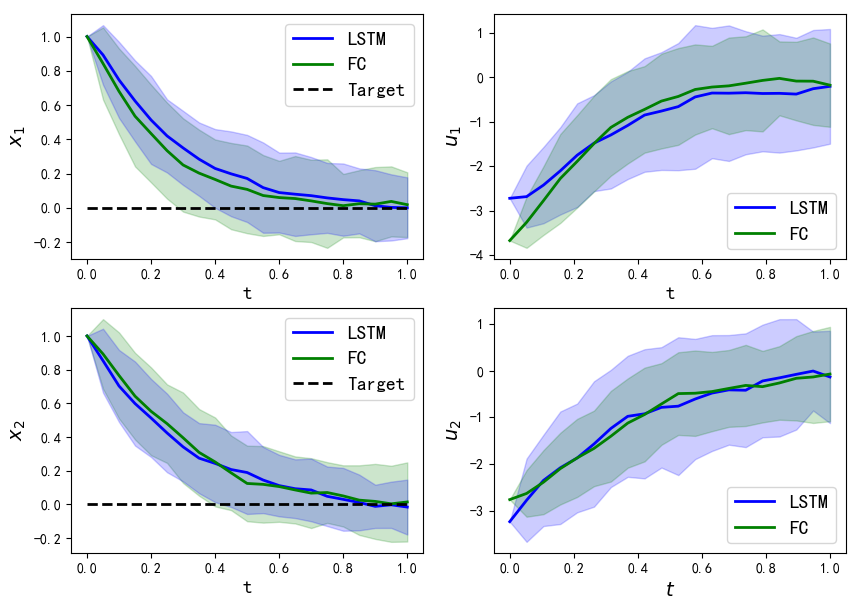
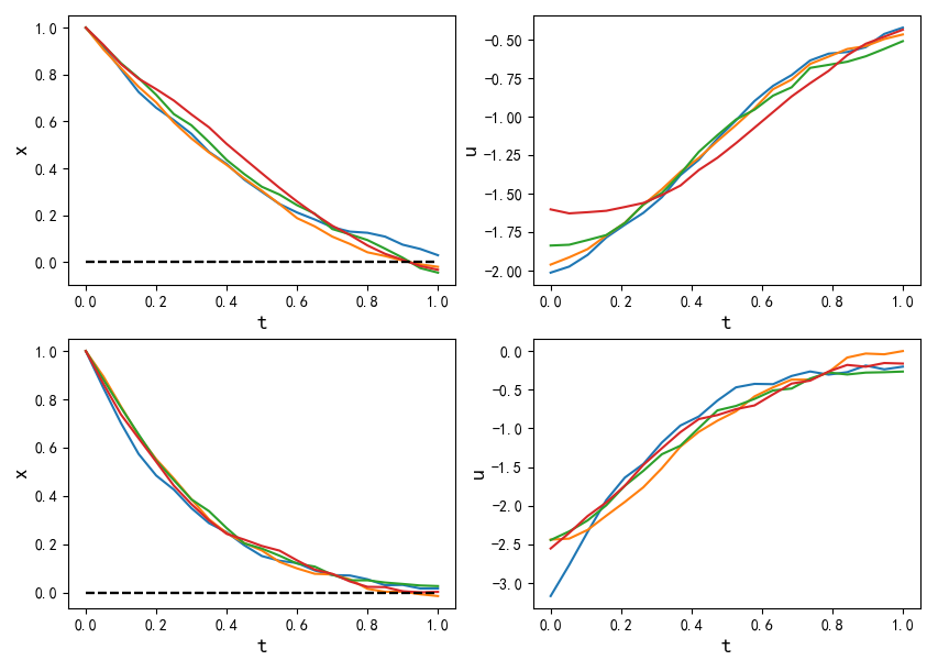
Figure 4: Numerical results of low-dimensional linear control problems. (a) $n=2$. Left: position $\mathbf{x}$; Right: control $\mathbf{u}$. (b) $n=4$. Upper: based on FC; Below: based on LSTM.

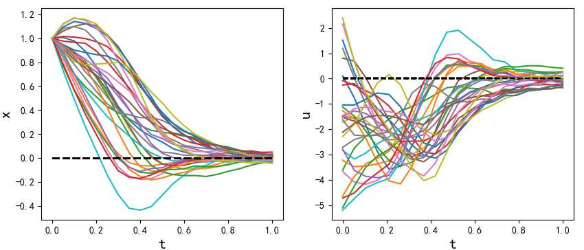
Figure 5: Numerical results of $30$-dimensional linear control problems based on LSTM. Left: position $\mathbf{x}$; Right: control $\mathbf{u}$.

6.3 Nonlinear control problems

In this section, we apply our DeepHJB solver to systems of pendulum, cart-pole and planner quadcopter for the task of reaching a final target. All the SOC problems for these systems can be formulated as the following form.

$$d\mathbf{x}_{t}=\left[f(\mathbf{x}_{t})+G(\mathbf{x}_{t})\mathbf{u}\right]dt+\lambda G(\mathbf{x}_{t})\mathbf{u}dw^{(1)}_{t}+Hdw^{(2)}_{t}.$$ (25)

with the cost functional (24). By Theorem 3.2, the controls in these problems have an explicit representation so that the DeepHJB solver with $1$-Net (Algorithm 2) will be utilized to solve these SOC problems.

Example 3. Consider the pendulum system

$$ml^{2}\ddot{\theta}+mgl\sin\theta+b\dot{\theta}=u$$

with $u\in\mathbb{R}$ the control torque input. We will use the transformation $\mathbf{x}=[\theta,\dot{\theta}]^{\top}$ and $\mathbf{u}=u$ to rewrite the pendulum system as the form (25) with

$$f(\mathbf{x}_{t})=\left(\begin{array}[]{c}\dot{\theta}\\ -\frac{l}{g}\sin\theta-\frac{b}{ml^{2}}\dot{\theta}\\ \end{array}\right),\quad G(\mathbf{x}_{t})=\left(\begin{array}[]{c}0\\ 1\\ \end{array}\right),\quad H=\left(\begin{array}[]{cc}0&0\\ 0&1\\ \end{array}\right).$$

The parameters utilized in the numerical experiment are given as follows.

$T$

$N$

$M$

$m$

$g$

$b$

$l$

$R$

$Q$

$Q_{T}$

$\lambda$

$\mathbf{x}_{0}$

$\mathbf{x}_{T}$

$2.0$

$40$

$50$

$1\mathrm{kg}$

$9.8\mathrm{m}/\mathrm{s}^{2}$

$1.2\mathrm{N}\cdot s$

$1.0\mathrm{m}$

$0.05\mathrm{I}_{2\times 2}$

$\mathrm{diag}[20,2]$

$\mathrm{diag}[100,50]$

$0.01$

$[\frac{\pi}{2},0]^{\top}$

$\mathbf{0}$

The pendulum states are illustrated in the top of Figure 6. It can be seen that the control task is completed with low variance and the DeepHJB solver with 1-Net conducted by FC and LSTM both performs well for the SOC problem of the pendulum system.

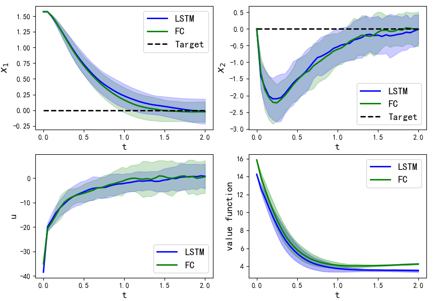
Figure 6: Numerical results of controlled pendulum system. Upper left: pendulum angle; Upper right: pendulum rate; Below left: the control; Below right: the value function.

Example 4. The cart-pole system

$$\left\{\begin{array}[]{ll}(m_{c}+m_{p})\ddot{x}+m_{p}l\ddot{\theta}\cos\theta-m_{p}l\dot{\theta}^{2}\sin\theta=u,\\ m_{p}l\ddot{x}\cos\theta+m_{p}l^{2}\ddot{\theta}+m_{p}gl\sin\theta=0,\end{array}\right.$$

where $u\in\mathbb{R}$ is the control force, $x$ is the horizontal position of the cart and $\theta$ is the counter-clockwise angle of the pendulum. By the transformation $\mathbf{q}=[x,\theta]^{\top}$, $\mathbf{x}=[\mathbf{q},\dot{\mathbf{q}}]^{\top}$ and $\mathbf{u}=u$, we rewrite the cart-pole system to the form (25) with

$$f(\mathbf{x}_{t})=\left(\begin{array}[]{c}\dot{x}\\ \dot{\theta}\\ \frac{m_{p}\sin\theta(l\dot{\theta}^{2}+g\cos\theta)}{m_{c}+m_{p}\sin^{2}\theta}\\ \frac{-m_{p}l\dot{\theta}^{2}\sin\theta\cos\theta-(m_{c}+m_{p})g\sin\theta}{l(m_{c}+m_{p}\sin^{2}\theta)}\\ \end{array}\right),\quad G(\mathbf{x}_{t})=\left(\begin{array}[]{c}0\\ 0\\ \frac{1}{m_{c}+m_{p}\sin^{2}\theta}\\ \frac{-1}{l(m_{c}+m_{p}\sin^{2}\theta)}\\ \end{array}\right),$$

$$H=\left(\begin{array}[]{cc}0_{2\times 2}&0_{2\times 2}\\ 0_{2\times 2}&0.1\mathrm{I}_{2\times 2}\\ \end{array}\right).$$

The following parameters are utilized to solve the SOC problem of the cart-pole system.

$T$	$N$	$M$	$m_{c}$	$m_{p}$	$g$	$l$	$R$	$Q=Q_{T}$	$\lambda$	$\mathbf{x}_{0}$	$\mathbf{x}_{T}$
$3.0$	$50$	$50$	$1\mathrm{kg}$	$0.01\mathrm{kg}$	$9.8\mathrm{m}/\mathrm{s}^{2}$	$1\mathrm{m}$	$0.05\mathrm{I}_{4\times 4}$	$\mathrm{diag}[\cdot,8.0,1.2,0.2]$	$0.03$	$\mathbf{0}$	$[\cdot,\pi,0,0]^{\mathrm{T}}$

Figure 7 demonstrates the cart-pole states which are computed by the DeepHJB solver with 1-Net based on LSTM. The swing-up task to stabilize the unstable fixed point $\mathbf{x}_{T}$ at $T=3$ is completed with low variance. Another interesting observation is that FC architecture is invalid in the experiment.

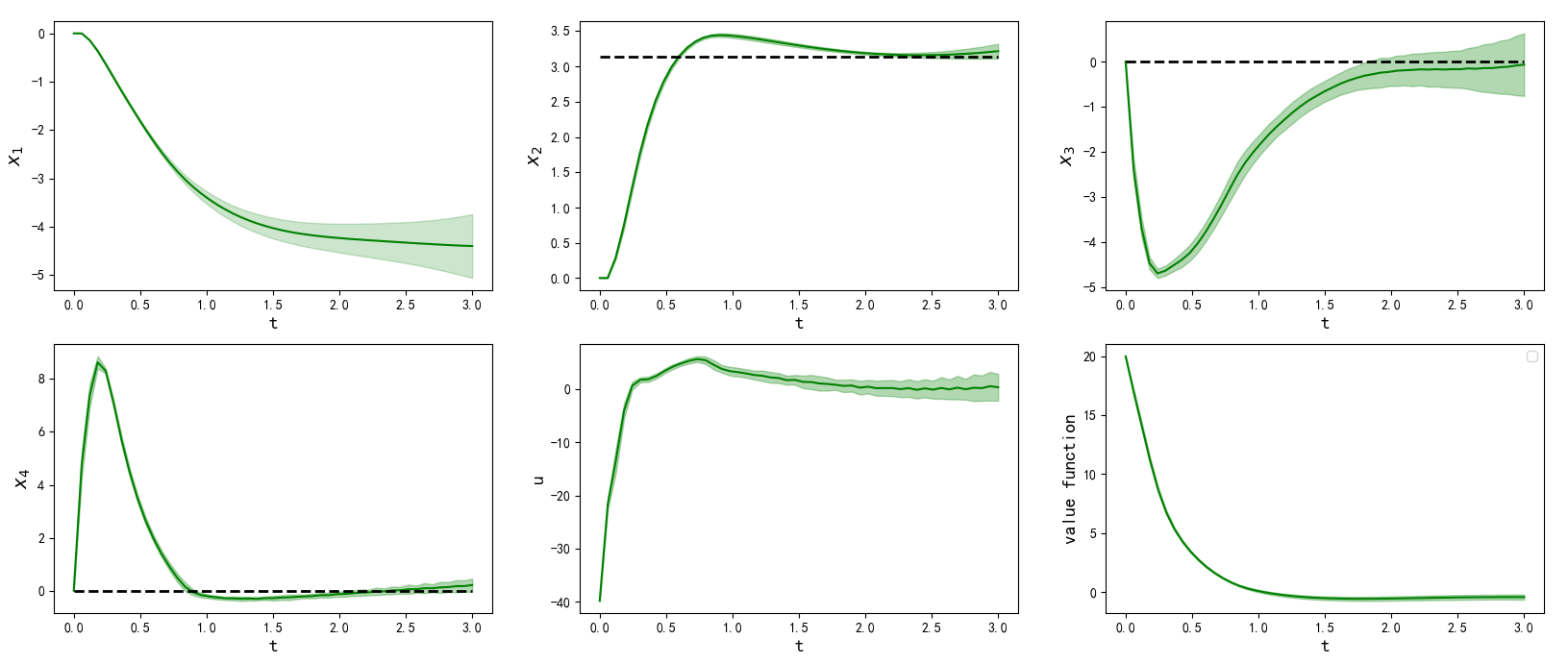
Figure 7: Numerical results of controlled cart-ploe system based on LSTM. Upper left: cart position; Upper middle: cart velocity; Upper right: pole angle; Below left: pole rate; Below middle: the control; Below right: the value function.

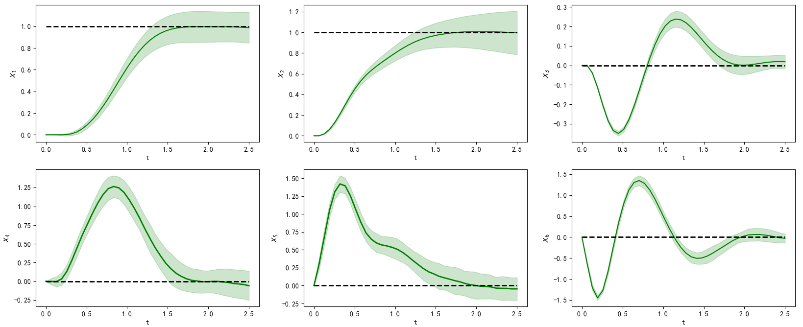
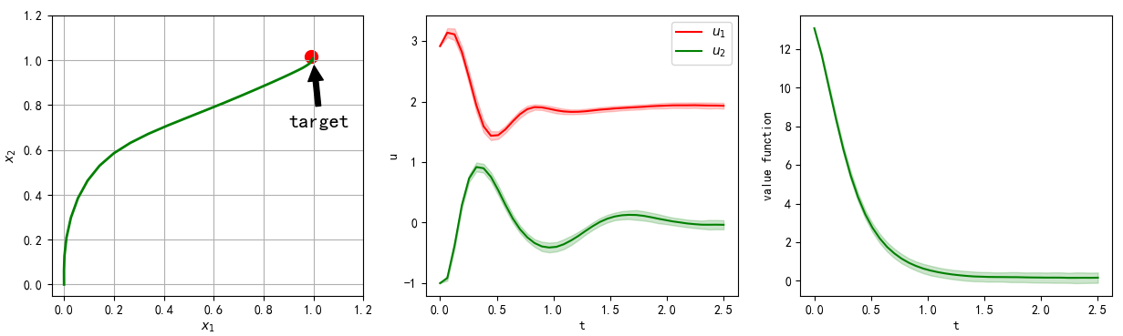
Figure 8: Numerical results of controlled planner quadcopter system based on LSTM. (a) Upper left: position $x$; Upper middle: position $y$; Upper right: angle; Below left: velocity along $x$-axis; Below middle: velocity along $y$-axis; Below right: angular velocity. (b) Left: the trajectory; Middle: the control; Right: the value function.

Example 5. The planar quadcopter can be modeled by

$$\left\{\begin{array}[]{ll}m\ddot{x}=-(v_{1}+v_{2})\sin\theta,\\ m\ddot{y}=(v_{1}+v_{2})\cos\theta-mg,\\ I\ddot{\theta}=r(v_{1}-v_{2}),\end{array}\right.$$

where $m$ is mass, $I$ the moment of inertia, and $r$ the distance from the center to the base of the propellor. In our analysis, we will use $\mathbf{q}=[x,y,\theta]^{\mathrm{T}}$, $\mathbf{x}=[\mathbf{q},\dot{\mathbf{q}}]^{\mathrm{T}}$. With the transformation $u_{1}=v_{1}+v_{2}$ and $u_{2}=r(v_{1}-v_{2})$, $\mathbf{u}=[u_{1},u_{2}]^{\mathrm{T}}$ denoting the command variables, the model of quadcopter system can be written as the form (25) with

$$f(\mathbf{x}_{t})=\left(\begin{array}[]{c}\dot{x}\\ \dot{y}\\ \dot{\theta}\\ 0\\ -g\\ 0\\ \end{array}\right),\quad G(\mathbf{x}_{t})=\left(\begin{array}[]{cc}0&0\\ 0&0\\ 0&0\\ -\frac{\sin\theta}{m}&0\\ \frac{\cos\theta}{m}&0\\ 0&\frac{1}{I}\\ \end{array}\right),\quad H=\left(\begin{array}[]{cc}0_{3\times 3}&0_{3\times 3}\\ 0_{3\times 3}&0.1\mathrm{I}_{3\times 3}\\ \end{array}\right).$$

The parameters of this SOC problem are listed as follows.

$T$	$N$	$M$	$m$	$g$	$r$	$I$	$R$	$Q=Q_{T}$	$\lambda$	$\mathbf{x}_{0}$	$\mathbf{x}_{T}$
$2.5$	$40$	$50$	$0.2\mathrm{kg}$	$9.8\mathrm{m}/\mathrm{s}^{2}$	$0.15\mathrm{m}$	$0.1\mathrm{kg}\cdot\mathrm{m}^{2}$	$1.5\mathrm{I}_{2\times 2}$	$\mathrm{diag}[8,8,12,0.5,0.5,0.5]$	$0.05$	$\mathbf{0}$	$[1,1,0,0,0,0]^{\top}$

Figure 8 shows the numerical results of the SOC problem for the planner quadcopter system. Similar to the cart-pole experiment, FC architecture is also invalid in this experiment. Simulations based on LSTM complete the control task with low variance, which is shown in Figure 8(a). In the left of Figure 8(b), the trajectory of the quadcopter from the initial point to the target position is illustrated.

6.4 Effect of some parameters

In our experiments, the physics-informed neural networks was trained by $30$ samples, while the networks in [38] was trained by $256$ samples. From the computational viewpoint, our algorithms are more efficient than the deep 2FBSDE algorithm proposed in [38]. In Figure 9, it is clear that the total errors of Algorithms 1 and 2, represented by the value of the loss, decrease with the increasing parameter of the time interval partition, which once more confirms the theoretical result in Theorem 5.1.

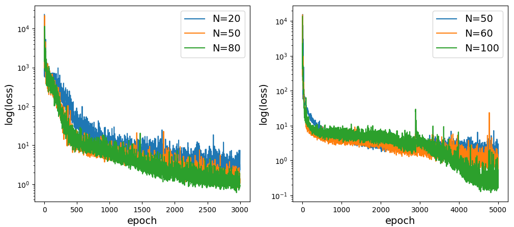
Figure 9: The values of the loss with varying parameter of the time interval partition. Left: the loss of Algorithm 1 implemented by LSTM in Example 1. Right: the loss of Algorithm 2 implemented by LSTM in Example 2 with $n=2$.

7 Conclusion

In this paper, we proposed the DeepHJB solver to solve finite time horizon SOC problems for a class of (non)linear systems. An detailed analysis is given on how the truncation, approximation and optimization errors have an influence on the accuracy of the DeepHJB solver. Furthermore, we apply our proposed solver to implement the stochastic optimal control for different models. It is observed that the DeepHJB solver can be conducted by the architecture of FC or LSTM. In Table 2, we summarize wether the network architecture is valid or not for different models. If both FC and LSTM can complete the control tasks for some SOC problems, a comparison of training time is shown in Figure 10.

models	dimension	LSTM	FC
linear model I	2	✓	✓
pendulum	2	✓	✓
linear model II	4	✓	✓
cart-pole	4	✓	✕
planner quadrotor	6	✓	✕
linear model III	30	✓	✕

Table 2: Summary on wether the network architecture is valid or not for different models.

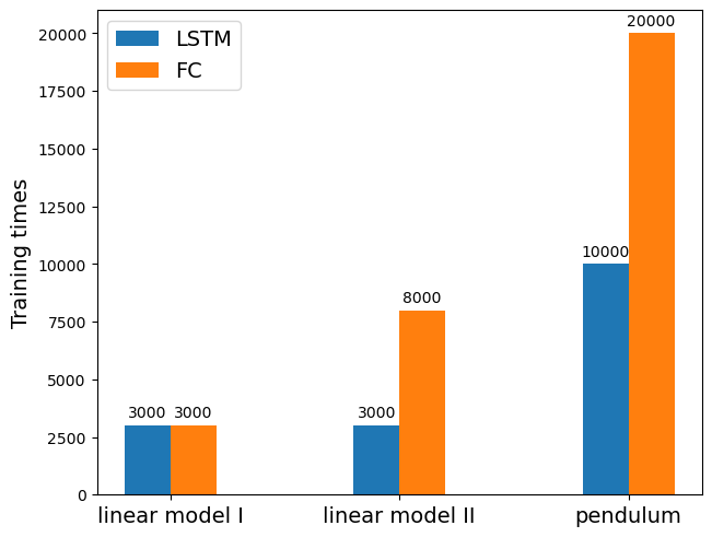
Figure 10: Comparing the training times of different network architectures

Although these theoretical results and numerical experiments in this work demonstrate the effectiveness of our DeepHJB solver, it still has plenty of room for development. For instance, how well the proposed solver performs for high-dimensional nonlinear problems remains an open question. Future work will be devoted to exploiting the present DeepHJB solver to investigate more deeply the control problems of high-dimensional nonlinear systems in practical applications.

Declaration of competing interest

The authors declare that they have no known competing financial interests or personal relationships that could have appeared to influence the work reported in this paper.

Data availability

The code developed in this work will be made available on request.

References

• [1] E. Todorov, Optimality principles in sensorimotor control, Nature Neuroscience 7 (2004) 907–915.
• [2] B. Berret, F. Jean, Efficient computation of optimal open-loop controls for stochastic systems, Automatica 115 (2020) 108874.
• [3] T. Russ, Robotic Manipulation: Perception, Planning, and Control, Draft textbook, 2023.
• [4] J.-M. Bismut, An introductory approach to duality in optimal stochastic control, SIAM Review 20 (1) (1978) 62–78.
• [5] A. Bensoussan, Stochastic maximum principle for distributed parameter system, Journal of the Franklin Institute 315 (5-6) (1983) 387–406.
• [6] L. S. Pontrygin, Mathematical Theory of Optimal Processes, CRC Press, 1987.
• [7] L. S. Pontrygin, Dynamic programming and stochastic control processes, Information and Control 1 (3) (1958) 228–239.
• [8] J. J. Douglas, J. Ma, P. Protter, Numerical methods for forward-backward stochastic differential equations, Annals of Applied Probability 6 (3) (1996) 940–968.
• [9] M. D. Giacinto, Numerical methods in financial and actuarial applications: a stochastic maximum principle approach, Journal of Mathematical Finance 8 (2018) 283–301.
• [10] J. Yong, Forward-backward stochastic differential equations: Initiation, development and beyond, Numerical Algebra, Control and Optimization 13 (3&4) (2023) 367–391.
• [11] N. Krylov, The rate of convergence of finite-difference approximations for Bellman equations with lipschitz coefficients, Applied Mathematics and Optimization 52 (3) (2005) 365–399.
• [12] W. McEneaney, Error analysis of a max-plus algorithm for a first-order HJB equation, in: Stochastic Theory and Control, 2002.
• [13] E. Theodorou, Y. Tassa, E. Todorov, Stochastic differential dynamic programming, in: American Control Conference, 2010.
• [14] H. Kappen, Linear theory for control of nonlinear stochastic systems, Physical Review Letters 95 (20) (2005) 200201.
• [15] K. Dvijotham, E. Todorov, Linearly solvable optimal control, in: Reinforcement Learning and Approximate Dynamic Programming for Feedback Control, 2012.
• [16] M. Horowitz, A. Damle, J. Burdick, Linear Hamilton–Jacobi–Bellman equations in high dimensions, in: 53rd IEEE conference on decision and control, 2014.
• [17] I. Exarchos, E. A. Theodorou, Stochastic optimal control via forward and backward stochastic differential equations and importance sampling, Automatica 87 (2018) 159–165.
• [18] P. J. Frey, P.-L. George, Mesh Generation: Application to Finite Elements, Hermes Science, 2000.
• [19] A. Szpiro, P. Dupuis, Second order numerical methods for first order Hamilton–Jacobi equations, SIAM Journal on Numerical Analysis 40 (3) (2002) 1136–1183.
• [20] J. Han, W. E, A. Jentzen, Deep learning-based numerical methods for high-dimensional parabolic partial differential equations and backward stochastic differential equations, Communications in Mathematics and Statistics 5 (4) (2017) 349–380.
• [21] J. Han, A. Jentzen, W. E, Solving high-dimensional partial differential equations using deep learning, Proceedings of the National Academy of Sciences 115 (34) (2018) 8505–8510.
• [22] C. Beck, S. Becker, P. Grohs, N. Jaafari, A. Jentzen, Solving the Kolmogorov PDE by means of deep learning, Journal of Scientific Computing 88 (2021) 73.
• [23] C. Huré, H. Pham, X. Warin, Deep backward schemes for high-dimensional nonlinear PDEs, Mathematics of Computation 8 (16) (2020) 1547–1579.
• [24] H. Pham, X. Warin, M. Germain, Neural networks-based backward scheme for fully nonlinear PDEs, arXiv:1908.00412.
• [25] C. Beck, S. Becker, P. Cheridito, A. Jentzen, A. Neufeld, Deep splitting method for parabolic PDEs, SIAM Journal on Scientific Computing 43 (5) (2021) A3135–A3154.
• [26] M. Germain, H. Pham, X. Warin, Approximation error analysis of some deep backward schemes for nonlinear PDEs, SIAM Journal on Scientific Computing 44 (1) (2022) A28–A56.
• [27] J. Sirignano, K. Spiliopoulos, DGM: A deep learning algorithm for solving partial differential equations, Journal of Computational Physics 375 (2018) 1339–1364.
• [28] M. Raissi, P. Perdikaris, G. E. Karniadakis, Physics-informed neural networks: A deep learning framework for solving forward and inverse problems involving nonlinear partial differential equations, Journal of Computational Physics 378 (2019) 686–707.
• [29] S. Cuomo, V. S. Di Cola, F. Giampaolo, G. Rozza, M. Raissi, F. Piccialli, Scientific machine learning through physics-informed neural networks: Where we are and what’s next, Journal of Scientific Computing 92 (2022) 88.
• [30] L. Lu, P. Jin, G. Pang, Z. Zhang, K. G. Em, Learning nonlinear operators via DeepONet based on the universal approximation theorem of operators, Nature Machine Intelligence 3 (2021) 218–229.
• [31] Z. Li, N. Kovachki, K. Azizzadenesheli, B. Liu, K. Bhattacharya, A. Stuart, A. Anandkumar, Fourier neural operator for parametric partial differential equations, in: International Conference on Learning Representations, 2021.
• [32] J.-P. Fouque, Z. Zhang, Deep learning methods for mean field control problems with delay, Frontiers in Applied Mathematics and Statistics 6 (2020) 11.
• [33] R. Carmona, M. Lauriére, Convergence analysis of machine learning algorithms for the numerical solution of mean field control and games II: the finite horizon case, Annals of Applied Probability 32 (6) (2022) 4065–4105.
• [34] S. Jin, S. Peng, Y. Peng, X. Zhang, Solving stochastic optimal control problem via stochastic maximum principle with deep learning method, Journal of Scientific Computing 93 (2022) 30.
• [35] C. Huré, H. Pham, A. Bachouch, N. Langrené, Deep neural networks algorithms for stochastic control problems on finite horizon: Convergence analysis, SIAM Journal on Numerical Analysis 59 (1) (2021) 525–557.
• [36] A. Bachouch, C. Huré, N. Langrené, H. Pham, Deep neural networks algorithms for stochastic control problems on finite horizon: Numerical applications, Methodology and Computing in Applied Probability 24 (1) (2022) 143–178.
• [37] M. Pereira, Z. Wang, T. Chen, E. Reed, E. Theodorou, Feynman-Kac neural network architectures for stochastic control using second-order fbsde theory, in: Proceedings of the 2nd Conference on Learning for Dynamics and Control, 2020.
• [38] Z. Wang, M. Pereira, T. Chen, E. Theodorou, E. Reed, Deep 2FBSDEs for systems with control multiplicative noise, arXiv:1906.04762.
• [39] J. Yong, X. Y. Zhou, Stochastic Controls, Springer, 1991.
• [40] W. Fleming, M. Soner, Controlled Markov Processes and Viscosity Solutions, Springer, 2006.
• [41] P. E. Kloeden, E. Platen, Numerical Solution of Stochastic Differential Equations, Springer, 1999.
• [42] S. Haykin, Neural Networks and Learning Machines, Pearson, 2009.