[table]capposition=top
Inference for Regression with
Variables Generated from Unstructured Data††thanks: Authors are listed in alphabetical order. This paper first circulated without TC as co-author under the title “Hamiltonian Monte Carlo for Regression with High-Dimensional Categorical Data” (https://doi.org/10.48550/arXiv.2107.08112) which was the second chapter of SS’s PhD thesis. SH acknowledges funding from ERC Consolidator Grant 864863, which supported his and LB’s time. We thank David Rossell for feedback, as well as seminar and workshop participants at Barcelona School of Economics, Columbia University, and the 3rd Monash-Warwick-Zurich Text-as-Data Workshop. The authors also thank the NumPyro development team for their outstanding work.
Abstract
The leading strategy for analyzing unstructured data uses two steps. First, latent variables of economic interest are estimated with an upstream information retrieval model. Second, the estimates are treated as “data” in a downstream econometric model. We establish theoretical arguments for why this two-step strategy leads to biased inference in empirically plausible settings. More constructively, we propose a one-step strategy for valid inference that uses the upstream and downstream models jointly. The one-step strategy (i) substantially reduces bias in simulations; (ii) has quantitatively important effects in a leading application using CEO time-use data; and (iii) can be readily adapted by applied researchers.
JEL Codes: C11, C51, C55
Keywords: Unstructured Data, Information Retrieval, Topic Modeling, Hamiltonian Monte Carlo, Measurement Error
1 Introduction
As the amount of digitally recorded unstructured data continues to grow rapidly, empirical work in economics is increasingly incorporating it. The leading example of such data is text (Gentzkow et al., 2019a , Ash and Hansen, 2023), but others include surveys, images, and audio recordings. One of the primary applications of such data is to recover some latent variable of economic interest with an information retrieval (IR) model. Examples abound: Baker et al., (2016) measures economic policy uncertainty with newspaper text; Hoberg and Phillips, (2016) infers firms’ latent industries with corporate filings; Hansen et al., (2018) constructs measures of policy deliberation from Federal Open Market Committee (FOMC) transcripts; Magnolfi et al., (2022) uses survey data to measure product differentiation; Compiani et al., (2023) measures substitutability between products using Amazon text and image data; Gorodnichenko et al., (2023) measures tone-of-voice from audio recordings of FOMC press conferences; Gabaix et al., (2023) imputes firm characteristics from investor holdings data; Einav et al., (2022) infer patients’ health status from survey answers; Vafa et al., (2023) constructs a measure of labor market experience based on CVs. These derived measures are rarely an end in themselves. Rather, the motivation for constructing them is to study how the concept they proxy interacts with the economic environment. As such, they are typically plugged into downstream econometric models whose parameters are the main object of study. Importantly, the IR and econometric models are almost always treated as wholly separate, with the output of the former treated as “data” in the latter. We call this the two-step strategy.
While clearly a pragmatic initial approach, the two-step strategy has largely unknown statistical properties. On one hand, ignoring the upstream IR model in the downstream econometric model suggests a generated regressor problem (Pagan, 1984). On the other, results in the time-series literature suggest plugging-in estimated latent variables need not lead to inference problems (Stock and Watson, 2002, Bernanke et al., 2005, Bai and Ng, 2006). More generally, characterizing the statistical guarantees—or lack thereof—of the two-step strategy is an important step in establishing a more mature understanding of reliable inference methods for unstructured data, an area that is still in its infancy.
Our first contribution is to provide theoretical arguments for why the two-step strategy leads to biased inference on regression parameters in empirically plausible settings. We consider a set of observations of quantitative and unstructured data. Each unstructured observation is composed of a high-dimensional vector of feature counts,111For example, one of the simplest representations of a textual corpus is the bag-of-words model in which each document is represented as a vector of integer counts over the unique vocabulary terms in the corpus. Even relatively small corpora contain thousands of unique dimensions. Moreover, the dimensionality grows even further as one consider richer linguistic units than individual words. More generally, many unstructured datasets can be represented as high-dimensional, categorical data. where is the amount of unstructured data for observation . The relative magnitudes of versus moments of play a key role in our analysis. We next specify a statistical model with three parts: a distribution over the feature-count vectors; a low-dimensional, latent variable representation for each such distribution; and a regression of an observed outcome variable onto the latent variables. The two-step strategy (i) estimates the latent variables from the observed feature counts, then (ii) regresses the outcome variable onto these estimates. This procedure mimics the common approach in the empirical literature described above. Our primary theoretical question is: under what conditions do the estimated coefficients and standard errors from (ii) allow for valid inference?
The basic problem is measurement error: the regressors in step (ii) contain estimated rather than true latent variables. As is well known, measurement error leads to biased point estimates and distorted standard errors, both of which are present as the number of observations grows with a fixed amount of unstructured data per observation. To capture a more empirically realistic situation, we allow and the distribution of to grow together so that both sampling error and measurement error are relevant for inference.222This framework is motivated by the observation that both sample size and the amount of unstructured data per observation are typically large in applications. Conventional fixed-DGP asymptotics provide poor approximations to this case. Our use of sequences of DGPs to get better asymptotic approximations to finite-sample behavior is similar in spirit to the weak instrument literature (Staiger and Stock, 1997), earlier work on measurement error (Chesher, 1991), and unit root testing (Phillips, 1987). Our main finding is that, whenever tends to a constant , there is a bias present in the asymptotic distribution of the regression coefficients which is increasing in . Larger values of give relatively greater importance to measurement error, and hence a larger bias. However, the asymptotic variance is the same as that from regression onto the true latent variables and the usual OLS standard errors are consistent. Hence, treating the estimated latent variables as observed data in the regression does not distort the width of confidence intervals, but centers them away from the truth. This contrasts with the generated regressor literature, which emphasizes the variance distortion arising from treating plug-in estimates as data.333In the classic generated regressor problem (Pagan, 1984) there is a common finite-dimensional parameter estimated in the first stage whereas here all latent covariates are estimated. Only when , so that sampling error dominates measurement error, does the two-step strategy allow for valid inference.
Of course, describes limiting behavior and cannot be used to directly compute the magnitude of the bias in a given finite dataset. But our theoretical arguments provide insight into when this bias is potentially problematic. Take, for example, job postings data as recorded by Lightcast (formerly Burning Glass), which has been used in dozens of papers. In 2022, there were 45 million individual job postings in the United States, with an average inverse posting length of 0.003. The empirical analogue of is , suggesting that measurement error may be large relative to sampling error. Another insight of the theory is that the magnitude of the bias arises not from the average amount of unstructured data per observation but rather the average inverse amount. So, if a dataset has a long tail of observations with little data, a bias can arise even if there is a substantial amount of data per observation on average. Again taking the Lightcast data, the average document size is . If one used in place of to compute the analogue of , would fall to below , highlighting the role of this tail behavior in driving measurement error bias. Nor is the Lightcast data a special case. There were patents filed to the US Patent and Trademark Office in 2023 and their summary texts have an average inverse document length of 0.002, so the analogue of is above . The calculation based instead on the inverse of the average document length is . Of course, there are other cases where one may have few total observations but with each individual observation having a large amount of unstructured data.444This case is similar to that typically considered in the literature on factor-augmented regression, which extracts common factors from time series and plugs them into downstream regressions. There are typically dozens or hundreds of time series per time unit, but limited observations per series. In our setting, (respectively ) is analogous to (respectively ). Bai and Ng, (2006) show that factor augmentation leads to valid inference when , analogous to . Because the exact magnitude of the problem is hard to assess in any given setting, it is important to develop robust inference methods that guard against measurement error whenever it may be present, but still allow reliable inference when it is not.
Our second contribution is to propose such an inference method: directly use the model’s joint distribution over unstructured data, latent variables, and numeric outcomes to perform maximum likelihood estimation. We refer to this as the one-step strategy.
While implementing the one-step strategy is straightforward theoretically, it presents a major computational challenge due to the large number of observation-specific latent variables that must be integrated out. To address this, we use Hamiltonian Monte Carlo (HMC; MacKay, 2003, Neal, 2012), a Markov Chain Monte Carlo algorithm that uses information on the gradient of a distribution to sample from it. Implementation is greatly simplified with the use of modern probabilistic programming languages: one simply specifies the likelihood in code, which is then “automatically” compiled to perform sampling. This paradigm is useful for applied researchers because it allows one to focus on model development without the need to re-write the estimation and inference algorithms each time the model is changed.555Previous papers that have performed inference using the joint likelihood approach with unstructured data include Gentzkow et al., 2019b , Ruiz et al., (2020), and Munro and Ng, (2022). These typically require extensive code to estimate, which makes adapting the model difficult for non-specialists. The most common probabilistic programming language in applied econometrics is Stan (Carpenter et al., 2017), which has been used by, for example, Meager, (2019) and Bandiera et al., (2021). Such applications have been limited to simple Bayesian meta-analyses with a few dozen parameters. Instead, we use the NumPyro package (Bingham et al., 2018, Phan et al., 2019), which efficiently computes the gradients that underlie HMC by using massive parallelization on dedicated hardware.
Third, we compare the performance of the two-step and one-step strategies in an applied setting. To this end, we introduce the Supervised Topic Model with Covariates (STMC) which combines elements of existing models (Blei et al., 2003, Roberts et al., 2014, Ahrens et al., 2021) but is, to the best of our knowledge, a new statistical model of unstructured data. The model reduces the dimensionality of feature-count vectors by projecting them onto a set of latent factors (or topics), as in Probabilistic Latent Semantic Analysis (Hofmann, 1999) and Latent Dirichlet Allocation (Blei et al., 2003). The dependence of outcome variables on latent factor loadings and observed covariates is captured by a “downstream” regression model. Additionally, the factor loadings can depend on a potentially different set of covariates via a second “upstream” regression model. All components are woven together by a joint likelihood. Specifying the model in code takes fewer than 25 lines, illustrating how one can perform automatic inference in a new setting that would previously have required a bespoke and complex codebase.
Many important research questions can be addressed with STMC. Suppose each unstructured observation is a monetary policy speech. One latent topic might have an interpretation as price rises, so its loadings represent how much each speech discusses price rises. A first research question, which can be addressed with the downstream model, might ask how speakers’ attention to price rises is related to their policy actions. A second research question might ask how policymakers’ backgrounds relate to the attention they devote to price rises. That question can be addressed with the upstream model.
In simulated data, we show that the two-step strategy produces estimates that exhibit a bias which is increasing in . Moreover, two-step confidence interval widths are similar to those obtained using the true latent variables as covariates. Both of these findings reinforce the main predictions of our theory. By contrast, the one-step strategy produces estimates that appear unbiased and the corresponding confidence intervals have the same widths as those using the true latent variables. Thus, one-step confidence intervals have both the correct width and the correct centering.
Next, we revisit the empirical application from Bandiera et al., (2020) which uses the two-step strategy to first estimate latent CEO behaviors from a CEO time-use survey, then explains firm performance using the estimated behaviors. The one-step strategy substantively changes estimates compared to the two-step strategy. For instance, the estimated effect of having an MBA degree on behavior more than doubles depending on whether the one-step or two-step strategy is used. To further test our theory, we next reduce the amount of unstructured data per observation and again deploy both inference strategies. This increases measurement error in latent behavior, and hence should increase the bias of the two-step strategy. Since the one-step strategy is always unbiased (asymptotically), one should observe larger differences in estimates, which is what we find. The estimated impact of behavior on firm performance, equivalent for both methods in the original data, is now over twice as large under the one-step strategy. Moreover, under the one-step strategy, the estimated effect sizes on behavior of having an MBA degree and of managing a large firm now triple.
Our overall message is that a popular way of using unstructured data in empirical work may suffer from measurement error which biases inference. We are unaware of other papers that explicitly model the source of this error, and how it relates to sampling error. Ultimately it is this trade-off (as manifested in ) that is most important for inference.666Fong and Tyler, (2021), Allon et al., (2023), and Zhang et al., (2023) all assume the existence of measurement error in a supervised learning algorithm used to generate regressors, but do not tie it to a specific model. Their proposed solution relies on a correctly labeled subset of data which can be used to build IV/GMM estimators. The one-step strategy requires no such labeled dataset to produce unbiased estimates. It can also be extended easily to handle non-linear models with measurement error. On a more positive note, though, a solution exists that is relatively easy to implement and computationally feasible. Since in practice researchers cannot characterize the severity of the measurement error in a given dataset, and there is little downside to applying the one-step strategy, we see it as a robust starting point for empirical analysis. We do note, however, that implementing the one-step strategy requires formulating a likelihood function. Latest-generation machine-learning- and AI-based approaches to information retrieval increasingly use neural networks with no obvious statistical structure that yields a likelihood function. A first comment is that, while implementing the one-step strategy may not be possible in these settings, the measurement error problem does not thereby disappear. Instead, it simply becomes harder to characterize statistically. Second, such approaches are often given statistical foundations following their adoption and, as this process plays out over the coming years, the scope for the one-step strategy will expand accordingly.777One illustrative example is the popular word2vec model for producing word embeddings. The original model (Mikolov et al., 2013b , Mikolov et al., 2013a ) had no statistical interpretation but yielded word representations that nevertheless captured semantic relationships well. Word2vec has subsequently been adopted by economists as part of the two-step strategy, for example to measure occupation-level exposure to technological change (Kogan et al., 2019) and emotionality in political speech (Gennaro and Ash, 2022). In parallel, a literature has developed likelihood-based interpretations of embeddings (Arora et al., 2016, Dieng et al., 2020, Ruiz et al., 2020) which could in principle be adapted for use in the one-step strategy. More generally, our belief is that inference problems arising from the analysis of unstructured data should be better recognized and taken more seriously in order to fully harness its potential value.
The rest of the paper proceeds as follows. Section 2 provides a simple setting in which the inference problems associated with the two-step strategy emerge. Section 3 further develops these arguments and presents our main theoretical results. Section 4 discusses instead the one-step strategy, associated computational tools, and introduces the Supervised Topic Model with Covariates. Section 5 presents simulation and empirical results comparing the two strategies. Section 6 concludes.
2 Motivating Example
This section presents a stylized model to illustrate clearly how the standard two-step strategy leads to biased inference in both the downstream and upstream models. The main take-aways from the stylized model are borne out in our empirical application.
2.1 Stylized Model
The stylized model is loosely based on the seminal work of Baker et al., (2016), which develops text-based measures of economic policy uncertainty (EPU) and investigates the relationship between EPU indices and economic outcomes. Suppose we are interested in the effect of (policy uncertainty in month ) on (employment or investment, say, in month ). We are primarily concerned with inference on in the regression model
| (1) |
Policy uncertainty itself is a nebulous concept that is difficult to precisely define let alone observe. The key innovation of Baker et al., (2016) is to construct EPU indices based on monthly counts of articles in 10 newspapers containing certain terms, then convert to index form. Their EPU index is then introduced as a covariate in regressions and VARs. But it’s arguably the case that their measure, while a strong signal of policy uncertainty, is not numerically the same as policy uncertainty. For instance, one could change the set of newspapers surveyed and obtain a quantitatively different (but related) measure. We therefore adopt the specification
| (2) |
where is the number of counts observed out of a sample of size and is the rate at which counts are expected. In the terminology of Baker et al., (2016), is the number of articles containing certain key terms in month , is the total number of articles that month, and is policy uncertainty that month. The variables , , and are observed but is not. One can estimate using , which is what Baker et al., (2016) do to construct their policy uncertainty measure.888See p. 1599 of Baker et al., (2016).
To facilitate the theoretical derivations below, let and , so the OLS estimator of would be consistent if were observed, and . To simplify derivations, we also assume (i) and are independent conditional on , and (ii) and are independent. These assumptions, which are credible in the context of Baker et al., (2016), are made primarily for convenience and can be relaxed. We assume the data are a random sample . Our analysis and findings extend easily to time-series data, though we stick to the IID case to simplify presentation.
2.2 Two-Step Strategy
In the context of this example, the usual two-step strategy would regress on and perform standard OLS inference for . This approach overlooks the fact that is a noisy estimate of . Failing to account for this measurement error problem may lead to biased estimates and inference.
Let denote the OLS estimator of from regressing of on . By standard OLS algebra, as the sample size we have
because and by the law of total variance and independence of and . Evidently, there is an attenuation bias caused by measurement error in which makes inconsistent.
The key determinant of bias is the average reciprocal amount of unstructured data per observation . If the amount of unstructured data per observation is large so that is small, we have
because for small . Hence, the bias is of the order of .
In many empirical settings, both measurement error and sampling error may play important roles. To shed light on the behavior of in this scenario, we consider a sequence of populations indexed by the sample size . The distribution of conditional on is fixed but the distribution of is changing with so that
| (3) |
This should not be interpreted literally as the data-generating process. Rather, it is a thought experiment to provide insights about how behaves when both measurement and sampling error are present. The parameter controls the relative importance of measurement error and sampling error: means sampling error swamps measurement error, while larger gives relatively greater importance to measurement error.
Proposition 1.
Consider the sequence of populations just described. Then
Proposition 1 shows that two-step inference is valid when . In this case, measurement error vanishes faster than sampling error and the estimated can be treated as if they are the true .
However, Proposition 1 also shows that two-step inference is invalid when . In this case, is consistent and its asymptotic variance is the same as if were regressed on the true , but the center of the asymptotic distribution is shifted due to the effect of measurement error. Confidence intervals based on standard OLS inference will therefore have approximately correct width but incorrect centering, meaning that their coverage rates will be below nominal coverage.999It follows from the general treatment in Section 3 that Eicker–Huber–White standard errors based on the estimated are consistent.
2.3 Upstream Inference
So far we have focused on the “downstream” regression model. Other research questions might involve inference in an “upstream” model linking variation in (policy uncertainty) to variation in an observed covariate (legislative gridlock, say). In that context, or some transformation of is the dependent variable in a regression on . Because is not observed, the two-step strategy would replace with in the regression. As before, the two-step strategy causes a measurement error problem, but now one that affects the dependent variable rather than the independent variable. As the measurement error is uncorrelated with , there would be no bias if were regressed on . But there can be a bias if a nonlinear transformation of is used as the dependent variable.
To illustrate this, consider the following setup. Because is supported on it is natural to transform it to have support using the log-odds ratio (or similar). Suppose we are concerned with inference on in the regression model
We again assume so that OLS would be unbiased if the true were observed. Because is latent, one could instead regress the empirical log odds ratio
on . Let denote the corresponding OLS estimator. To understand the forces at play, we study the behavior of in a sequence of populations where the distribution of is fixed but the distribution of varies with so that (3) holds. Like before, to facilitate derivations we assume and are independent conditional on , and and are independent.
Proposition 2 shows that two-step inference in the upstream model is valid when but invalid when . In the latter case, confidence intervals based on standard OLS inference will again have approximately correct width but incorrect centering, and will therefore have coverage below nominal coverage. The degree to which standard OLS confidence intervals under-cover depends partly on the size of . Because the function diverges to as approaches and , this covariance can be very large when the distribution of puts mass near zero and/or one. Thus, first-order bias can be large even when is small provided has sufficient mass in its tails.
3 Full Analysis of the Two-Step Strategy
One limiting feature of the stylized model in the previous section is that the observed data are not high-dimensional. In this section, we relax this and allow each unstructured data observation to lie in a high-dimensional space which requires some dimensionality reduction prior to regression analysis. In this section, we first describe the statistical framework linking unstructured data and the downstream regression model. We then analyze the usual two-step strategy and shed light on when it leads to valid inference, extending the findings from the stylized model in Section 2 to a general setting. In particular, two-step inference is valid only when the amount of unstructured data per observation is much larger than sample size, so that measurement error is of smaller order than sampling error. Otherwise, confidence intervals based on the usual two-step strategy have the correct width but incorrect centering, and therefore have coverage rates below nominal coverage. In the next section, we supplement the statistical framework with an upstream model linking covariates to the unstructured data to produce the Supervised Topic Model with Covariates and discuss how it solves some of these inference problems.
3.1 Statistical Framework
We begin by specifying a statistical model that, broadly speaking, has two parts. The first part computes low-dimensional numerical representations of the unstructured data. The second part introduces these numerical representations as covariates, potentially along with other quantitative data, into a linear regression model. There are a wide array of methods for dimensionality reduction used in the literature. We focus on factor modeling, which, in the context of high-dimensional discrete data, is also called topic modeling. We make this choice for two reasons. First, topic models have a well-defined statistical structure which facilitates theoretical analysis. Second, there is a large empirical literature which uses topic models as part of the two-step strategy, most commonly using textual data. Examples include Hansen et al., (2018), Mueller and Rauh, (2018), Larsen and Thorsrud, (2019), Thorsrud, (2020), Bybee et al., (2020), and Adams et al., (2021). However, the use of topic models is not limited to textual data. For example, Bandiera et al., (2020), Draca and Schwarz, (2021), and Munro and Ng, (2022) use topic models to analyze survey data. Meanwhile, Nimczik, (2017) and Olivella et al., (2021) use topic models for network-structured data.
3.1.1 Model
We consider a setting where each unstructured observation is described by , a -dimensional vector of count variables, where is the number of times a feature appears in observation . We consider to be high dimensional. This setting is not overly restrictive, as many types of unstructured data are naturally high-dimensional and discrete. For example, in the bag-of-words model is the number of unique terms in a textual corpus, typically in the thousands, and is the count of term in document . The first part of the model generates a -dimensional representation of , where . The second part introduces these low-dimensional representations as covariates, potentially along with other quantitative data , into a linear regression model:
| (4) |
In most empirical applications in economics and finance, the key parameters of interest are the regression coefficients. Hence, we will focus mainly on estimation and inference for in what follows.
The model we consider for the unstructured data is widely used in practice but also tractable enough that we can develop theory for why the two-step strategy leads to biased inference in empirically realistic settings. As is a vector of counts, it is without loss of generality to model it as a Multinomial distribution. We impose additional structure on the count probabilities for interpretability. The model is based on Probabilistic Latent Semantic Analysis (Hofmann, 1999, PLSA), a widely used factor model for discrete data, and its close cousin Latent Dirichlet Allocation (Blei et al., 2003, LDA). Formally,
| (5) |
where is the count of all features in observation —a measure of the amount of unstructured data for observation —and the count probabilities have a factor structure .101010This model nests as a special case a pure multinomial model where and . There are separate distributions over the features denoted where each lies in the -dimensional simplex. In text applications, these distributions are called topics, but more generally they represent common factors from which individual observations are built. We collect the factors into a row-stochastic matrix where . Each observation is characterized by the latent vector which lies in the -dimensional simplex. Its elements represent the weight attached to in generating . Hence, the count probabilities for observation are . It is helpful to think of as a matrix of common parameters and as an observation-specific latent random vector. The quantity determines the degree of precision with which we can infer from . The interplay between the distribution of and the number of observations plays an important role in our theory below.
Example: Monetary Policy Speeches.
Suppose each unstructured observation is a monetary policy speech. One distribution might put high weight on words like ‘inflation’, ‘prices’, and ‘cpi’, so would have an interpretation as price rises. The corresponding then represents how much speech discuss price rises. One research question might ask how attention paid to price rises, along with other economic conditions captured by other topics, affects policy actions. This could be captured by the coefficients in (4) where is the policy action of speaker and measures quantitative information like market forecasts for growth and inflation at the time the speech was made.
The main point beyond this specific example is that many research questions that seek to map variation across high-dimensional count observations as captured by a topic model into variation in some numeric variable will involve inference on .
3.1.2 Data and Maintained Assumptions
The data available are a random sample satisfying (4) and (5). We further assume that is independent of , , and , and that and are independent conditional on and . We emphasize that these restrictions are not essential and are made to simplify the following derivation. Our theory can easily be extended to time-series models, such as where (5) is replaced by a vector autoregression. We do not do so here, however, as the main take-aways are most clearly illustrated in the IID case.
We also assume that and the are identified in the sense that there is a unique decomposition with collecting the vectors of count probabilities across observations and collecting the topic weights across observations. For instance, identification is commonly achieved in text applications by assuming the existence of certain anchor words: these are words that are known to appear in certain topics but not others. We impose this identifiability condition because our objective is to analyze the consequences of the two-step inference approach in a transparent way. Adding partial identification into the mix will significantly complicate the analysis but may be an interesting extentsion in future research.
3.2 Theory for the Two-Step Strategy
The standard two-step strategy can be summarized as follows:
-
(i)
Estimates of are computed from the unstructured observations, e.g. by LDA.
-
(ii)
is regressed on and . Conventional OLS standard errors are reported, treating the as if they are regular numeric data.
Evidently there is a measurement error problem: the estimates are noisy proxies for the true appearing in the regression model (4). But Step (ii) overlooks this problem and treats the first-stage estimates as regular numeric data. This raises the possibility that OLS estimates of may be biased due to measurement error introduced in Step (i). Moreover, conventional standard errors are typically reported for inference on . These do not account for any additional variation introduced by using noisy instead of , raising the possibility that inference may be biased.
In this section, we use the above statistical framework to explore when this approach delivers valid estimates and inference for . To focus on the key conceptual issues, we abstract away from any additional covariates in the regression equation (4).111111This is not restrictive, as any additional numeric covariates can be partialled-out at the cost of more complicated notation. Similarly, the following analysis and findings extend easily to models where (4) is replaced by for some known matrix . See Section 3.3. Once is omitted the regression still contains an intercept because the elements of sum to one. In this simplified setting, the OLS estimator of is given by
| (6) |
3.2.1 Fixed Population
We first consider the large-sample properties of where the number of observations becomes large () but the distribution of is held fixed. This fixed-population asymptotic framework captures a setting where the amount of unstructured data per observation is small relative to the overall sample size, as commonly encountered in empirical work.
There are many different ways of estimating and in (5). For instance, one could use LDA (Blei et al., 2003) or more recent methods developed by Bing et al., (2020), Wu et al., (2023), Ke and Wang, (2022), and many others. As our objective is to focus on the consequences of the above two-step strategy, we abstract from algorithmic-specific details and instead impose some mild high-level conditions on the estimators of and of . Let denote the matrix of sample frequencies (or term frequencies, in text applications). Let denote convergence in probability as the number of observations becomes large.
Assumption 1.
-
(i)
and have full rank.
-
(ii)
.
-
(iii)
.
Assumption 1(i) says that there are no fewer than topics. We view this as a weak restriction as is typically much smaller than in applications. Assumption 1(ii) says that the estimator is consistent for the topic weights . This is a mild condition satisfied by many estimators for topic models. Assumption 1(iii) imposes some structure on the estimators that we leverage to derive the asymptotic properties of . Note that Assumption 1(iii) is not vacuous: we have (by Assumption 1(i)) so, given any consistent estimator of , one could estimate simply by setting . In that case, . Also note that the first condition in (i) and parts (ii) and (iii) hold trivially for the pure multinomial model because and .
Our first main result shows that the OLS estimator of in equation (6) is inconsistent in this fixed-population setting. Let denote a diagonal matrix whose diagonal elements are the elements of the vector .
Theorem 1.
The first part of Theorem 1 shows that the measurement error introduced by regressing on instead of the true (infeasible) makes the estimator inconsistent. How well we can impute the true latent for each observation depends on the amount of unstructured data . Because each is finite, each has a measurement error that doesn’t disappear when the number of observations becomes large. As a consequence, is biased (even asymptotically).
More constructively, Theorem 1 shows that what is important for controlling bias is not the average amount of unstructured data but rather the mean reciprocal amount . This makes intuitive sense, as the measurement error in decays with but the rate of decay decreases with . If the population contains a larger share of observations with small , then larger measurement errors in will be more prevalent and will have a larger bias121212To put it differently, increasing the amount of unstructured data for the observations with small will have a larger effect on the expected average size of the measurement error than if the additional data was collected for the observations with large . Consequently, the across-observation distribution of matters beyond its mean. It is important to emphasize that even if most observations have a large but a small mass do not (meaning that may still be large), then the noise in from the observations with small can still substantially bias .
The second part of Theorem 1 shows that when all observations have a large amount of unstructured data (so that is small), the first-order effect is a bias of size
Thus, the first-order effect of bias is proportional to .
3.2.2 Sequence of Populations
We now build on this insight to consider a sequence of populations where the amount of unstructured data per observation becomes larger as the sample size increases. This asymptotic framework is designed to shed light on how behaves when there is a relatively large number of observations and there is a large amount of unstructured data per observation. In this scenario, the measurement errors for each observation are small but their cumulative effect may not be completely ignorable relative to sampling error.
Formally, we consider a sequence of populations indexed by sample size . In each population, we keep the distribution of conditional on fixed and as described in Section 3.1. We also maintain the assumption that is given by the topic model (5). However, we let the marginal distribution of to change with the sample size to allow the amount of unstructured data per observation to become large as the sample size increases. Specifically, we consider a framework in which
| (7) |
as . The quantity plays a key role in the following analysis. Loosely speaking, represents the relative magnitudes of sampling error and measurement error.
The case corresponds to a setting in which the amount of unstructured data per observation is of much larger order than sample size. Consequently, measurement error is of smaller order (asymptotically) than sampling error. In this case, our theory implies that the two-step strategy leads to valid inference. That is, the measurement error introduced by regressing on instead of can effectively be ignored and standard inference can proceed treating the as if they are the true .
The case is the critical case in which there is a large, but not overwhelming, amount of unstructured data per observation. This case mimics many empirically realistic designs where measurement error and sampling error are both small but non-negligible. We show in this case that is consistent but standard two-step inference is invalid. In particular, the asymptotic distribution of has the correct variance but its center is shifted due to measurement error bias. Consequently, confidence intervals based on the usual two-step strategy have the correct width but incorrect centering, and therefore have a coverage rate that is smaller than nominal coverage.131313The case corresponds to a setting where measurement error is of larger order than sampling error. Here is consistent provided but two-step inference is invalid because bias is of larger order than sampling uncertainty. In that case, the coverage rates of standard OLS confidence intervals asymptote to zero as the sample size becomes large.
In what follows, notions of convergence in probability and distribution should be understood as holding along this sequence of populations satisfying (7).
Assumption 2.
-
(i)
, , and have full rank.
-
(ii)
.
-
(iii)
.
-
(iv)
for some .
-
(v)
almost surely for some .
Assumption 2(i) is mostly the same as Assumption 1(i) except we also require that has full rank so that the asymptotic variance of is well defined. Parts (ii) and (iii) strengthen parts (ii) and (iii) of Assumption 1 to require convergence a faster-than-root- rate. This is really to simplify the derivation: if convergence occurs instead at a root- rate, then additional terms may distort the asymptotic distribution further. Nevertheless we believe these two conditions are broadly satisfied. For instance, part (ii) is mild in view of known convergence rates established for estimators of .141414Bing et al., (2020), Wu et al., (2023), and Ke and Wang, (2022) derive finite-sample upper bounds for various estimators of . Each of their results implies the corresponding estimator converges at the optimal rate (up to log terms) where, for simplicity, the are all of the same order . Hence, all estimators converge faster than when grows with , as we have here by (7). As before, part (iii) is made to simplify the derivation but is also not vacuous: given any estimator proposed in the literature satisfying part (ii), one could construct directly by setting , in which case . As before, the first condition in (i) and parts (ii) and (iii) hold trivially for the pure multinomial model because and . Part (iv) is standard for inference for regression under conditional heteroskedasticity (e.g., White, (1980)). Finally, Part (v) is made to simplify technical derivations and can be relaxed. This assumption means that for each , is supported on for some constants . This condition is much weaker than the conventional assumption that all grow at the same rate (Bing et al., 2020, Wu et al., 2023, Ke and Wang, 2022) which, in view of (7), would imply that is supported on . This condition is only used to establish consistency of Eicker–Huber–White standard errors and is not required for asymptotic normality.
Our second main result shows that the OLS estimator of in equation (6) is consistent and derives its asymptotic distribution.
Theorem 2.
Theorem 2 shows that inference is valid when . In this case, we have
The OLS estimator obtained by regressing on therefore has the same asymptotic distribution as the (infeasible) OLS estimator obtained by regressing on the true latent . The reason is that corresponds to a scenario where measurement error is of smaller order than sampling error. Moreover, the usual Eicker–Huber–White standard errors computed using the estimates are consistent. Hence, measurement error can effectively be ignored when performing inference on .
At an abstract level, this case is analogous to asymptotic theory for factor-augmented regressions. In that setting, latent factors at each date are imputed from a vector of predictor variables , then the estimated factors are treated as covariates in a regression model. Bai and Ng, (2006) show that treating the estimated factors as if they are the true latent factors leads to valid inference provided , where is the time-series dimension and is the cross-sectional dimension. Their is analogous to our , their is analogous to our , and their is analogous to our . Hence, their condition is analogous to .
An important insight developed in Theorem 2 is that standard two-step inference is valid if and only if . If , then the asymptotic distribution of has the correct variance (which is consistently estimated by the usual Eicker–Huber–White standard errors) but its center is shifted due to measurement error bias.151515This is the opposite of a generated regressors problem (Pagan, 1984), where the asymptotic variance is inflated but there is no location shift. With generated regressors there is a common finite-dimensional parameter estimated in the first stage whereas here all covariates are estimated in the first stage. See Bai and Ng, (2006) for further discussion in the context of factor-augmented regressions. Consequently, confidence intervals have the correct width but incorrect centering, and therefore have coverage below their nominal coverage.
3.3 General Regression Model
The insights developed in Theorems 1 and 2 were presented for the basic regression model . We now show they extend to more general models of the form
| (10) |
where is a pre-specified matrix. For instance, may be known to depend only on a subset of topics corresponding to particular elements of , in which case picks off the relevant elements (topics).
By residual regression, we can write model (10) as
where and . Similarly, the least-squares estimator of in model (10) can be expressed
| (11) |
where .
Reasoning as in Theorem 1, the OLS estimator in (11) will be inconsistent in a fixed-population asymptotic framework where the amount of unstructured data per observation is small relative to the sample size .
Now consider a sequence-of-populations asymptotic framework where the distribution of unstructured data is allowed to grow with sample size as in (7). By a straightforward modification of the arguments in Theorem 2, the OLS estimator of in equation (11) is consistent and asymptotically normal, but with an incorrect centering when :
Two-step standard errors are also consistent, irrespective of whether or :
where .
Hence, as before, standard two-step inference on is valid if . But if , then standard two-step confidence intervals will have approximately correct width but incorrect centering and will therefore have coverage below nominal coverage.
4 One-Step Strategy
In this section, we first discuss from a theoretical perspective the one-step strategy for inference that overcomes the bias from the two-step strategy. While the idea is generic, for concreteness we develop it within a specific model we call the Supervised Topic Model with Covariates which extends the model presented in the previous section. Second, we discuss the computational challenge of implementing the one-step strategy, which we solve with Hamiltonian Monte Carlo (HMC) deployed on modern hardware systems. This allows for highly scalable inference with minimal coding. More in-depth overviews of HMC are provided in Neal, (2012), Hoffman and Gelman, (2014), and Betancourt, (2018). We are not aware of the application of HMC to topic models in the literature.
4.1 Supervised Topic Model with Covariates
The model for illustrating the one-step strategy again features the downstream regression model (4) and the upstream topic model (5). But we further enrich the model to include a probabilistic relationship between the topic shares and a vector of covariates . The covariates may or may not be the same as . We allow these additional dependencies to enhance the applicability of the model, and to demonstrate how our computational approach can perform inference for even complex models with relative ease.
Example: Monetary Policy Speeches (Continued).
To return to the example of Section 3, the downstream regression model (4) could capture how policymakers’ attention predicts policy actions controlling for economic conditions. But policymakers’ attention can itself be a function of speaker characteristics such as demographic variables, or past experience of economic conditions (Malmendier et al., 2021). Such variables would enter but arguably not directly affect policy decisions beyond their effect on attention; i.e., they would not enter .
To capture dependence between and , we specify the distribution of conditional on as logistic normal, though other specifications could also be used. The full model, which we call the Supervised Topic Model with Covariates (STMC), is specified in Model 1.
| (Upstream Topic Model) | |||
| (Downstream Regression Model) |
The additional parameters in Model 1 are a matrix of coefficients and scale parameters and . The th row of , denoted , captures how variation in covariates maps to variation in the prevalence of the th topic across observations. Hence, a number of research questions can be addressed by performing inference on . While we have modeled the error terms in the downstream regression and upstream logistic normal as homoskedastic to simplify presentation, this can easily be relaxed. Similarly, the logistic normal and normal specifications can also be substituted for other distributions or quasi-distributions as appropriate. For instance, one could use the sandwich quasi-likelihood of Müller, (2013).
To our knowledge, STMC is new in the literature. Roberts et al., (2014) presents a model in which a logistic normal distribution over is parameterized by covariates but without a downstream regression. Blei and McAuliffe, (2010) and Ahrens et al., (2021) present models in which linear combinations of topic shares explain a response variable, but do not allow covariates to enter the distribution over . As such, we view STMC as of independent interest in the literature on topic modeling, although its primary purpose is to provide an example in which dimensionality reduction and linear regression are part of the same joint model and one cares about doing valid inference on model parameters.
4.2 Inference Approach for One-Step Strategy
The components of Model 1 combine to give a likelihood for , , and conditional on and covariates and . As is latent, we can integrate it out to obtain a likelihood depending only on observable variables, which can then be used for maximum likelihood estimation of model parameters . However, there are two challenges. First, the integration has no closed-form solution and so must be performed numerically. Moreover, this numerical integration is high-dimensional and must be done observation-by-observation. As such, standard likelihood-based estimation is not computationally feasible.
The inference approach we take, while frequentist, is instead based on Bayesian computation. The integration step is performed implicitly as part of the sampling procedure. Similar approaches are taken to deal with latent states in Bayesian estimation of DSGE models (Herbst and Schorfheide, 2016). In this approach, Model 1 is supplemented with a prior for . The latent are themselves treated as “parameters”, with the logistic normal component of Model 1 acting as their prior. We sample from the posterior distribution for and the given the observed data . The marginal draws for represent draws from the posterior distribution for based on the integrated likelihood .
It is important to emphasize that while our approach uses Bayesian computation, one does in fact perform valid frequentist inference on model parameters using this method. The maximum likelihood estimator of is asymptotically normal under standard regularity conditions (e.g., Theorem 5.41 of van der Vaart, 1998). By the Bernstein–von Mises Theorem (see Theorem 10.1 of van der Vaart, 1998 and discussion), the posterior mean of is first-order asymptotically equivalent to the MLE . Moreover, the posterior distribution of is asymptotically normal with mean and variance (when appropriately scaled with ) equal to the asymptotic variance of the MLE. As such, Bayesian credible sets for —or any of its components such as —are valid frequentist confidence sets with the desired asymptotic coverage. This approach is also efficient for inference on and its components, as it is asymptotically equivalent to likelihood-based inference.
Following the literature on topic modeling, we specify the following standard prior distributions for model parameters:
| (Priors) | ||||
If one so desires, these priors can be changed with one line of code in our implementation of the inference algorithm explained below. In total, the model has eight hyperparameters: the three terms in (Priors) as well as in (Upstream Topic Model); the symmetric Dirichlet parameter in (Priors); the two Gamma distribution parameters in (Priors).
We emphasize again that the model and priors serve primarily as an illustration. An interested researcher should be able to modify it as needed to accommodate different data; to test robustness of the conclusions to specifying alternative distributions for the data; or to test robustness with respect to choice of priors. The key is to avoid having to re-derive complex inference algorithms every time the model is adjusted, and this is precisely the main advantage of automatic inference methods we now describe.
4.3 Overview of the HMC Algorithm
Our problem is to sample from the posterior distribution where are the STMC parameters. To do so, we use Hamiltonian Monte Carlo (HMC), a modern Markov chain Monte Carlo (MCMC) algorithm that is particularly well-suited to high-dimensional models.161616Gibbs sampling is often used in the topic modeling literature (Griffiths and Steyvers, 2004). This is difficult to implement for STMC because (i) the logistic normal prior is not conjugate to the multinomial distribution and (ii) there are a large number of parameters in the model in realistic use cases. MCMC algorithms define a stochastic process, i.e., a Markov chain, whose ergodic distribution coincides with the posterior distribution one wishes to sample from. Samples from this Markov chain can be used to form estimates of interest, e.g. the expected value of a model parameter under the posterior distribution, as in Monte Carlo simulation. Efficient MCMC algorithms have low autocorrelation across samples which improves the accuracy of the resulting estimates.
A popular and simple MCMC method is the Metropolis-Hastings (MH) algorithm. Note the posterior is proportional to , which is formed by multiplying the likelihood by the prior. The MH algorithm generates samples from the posterior in two steps: (1) propose a new state from the current state using a pre-specified proposal distribution; then (2) accept the new proposal with a probability that increases in the ratio . A challenge in practice is that the proposal distribution must be chosen carefully to avoid slow convergence. Taking small steps in a random direction can have a high acceptance probability but also high autocorrelation across samples and slow convergence. Taking a large step in a random direction can drastically reduce and hence the acceptance probability.
The HMC algorithm addresses this problem by utilizing the geometry of to propose distant states that nonetheless have high chance of acceptance. This is achieved by proposing a new state by following Hamiltonian dynamics for a certain number of steps, starting from the initial state . This process is determined by the curvature of , and so determining the path to follow requires evaluating the gradient of with respect to the parameters . The specific variant of HMC that we use is the No-U-Turn Sampler (Hoffman and Gelman, 2014, NUTS). The intuitive idea of NUTS is to follow the Hamiltonian dynamics for a random number of steps, and to stop when the path starts to double back on itself. This is not only more efficient than following the dynamics for a fixed number of steps, but also avoids the need to specify the number of steps in advance.
4.4 HMC and Probabilistic Programming
From an implementation perspective, an advantage of HMC is that it is amenable to probabilistic programming. This allows one to define a data generating process for a statistical model in computer code, after which sampling is performed “automatically” in the background by following a generic set of algorithmic procedures adapted to the given model. In practice, modern probabilistic programming libraries use automatic differentiation to compute the gradients of highly flexible families of densities. Furthermore, the density and gradient computations are typically parallelizable as they are additive with respect to the data points.171717More precisely, the logarithm of is additive with respect to the data points, and the gradient of the logarithm of is the sum of the gradients of the log-likelihood and the logarithm of the prior. This facilitates the use of the same specialized hardware normally used for machine learning tasks.
NUTS is implemented in many probabilistic programming libraries, the most popular of which is Stan. For this paper, we instead use NumPyro (Phan et al., 2019), which utilizes a state-of-the-art automatic differentiation engine Jax (Bradbury et al., 2018) and allows users to easily deploy these computations to specialized hardware such as Graphical Processing Units (GPUs) and Tensor Processing Units (TPUs), resulting in a dramatic improvement in computation time. Furthermore, NumPyro is a Python library, not a standalone program, which means that it is easy to integrate with other libraries and benefits from the host of functionalities that Python provides. This said, our goal is not to advocate for any particular library, but to demonstrate that software and hardware have evolved to a point that allows Bayesian computation to be performed at scale without the need to manually derive sampling equations.
The NumPyro code needed to draw samples from the posterior distribution of STMC is only several dozen lines long, and individual elements can be quickly modified to specify alternative distributional assumptions or new models.
5 Empirical Results
In theory, the one-step strategy should outperform the two-step strategy, but establishing the empirical relevance of the bias that the latter produces is clearly important. While our computational approach makes the one-step strategy straightforward to implement, easier still would be for applied researchers to continue to use off-the-shelf packages for information retrieval and then to import the outputs into familiar regression software. This section establishes that there is indeed a quantitatively meaningful difference in regression parameter estimates produced by the two methods, both in simulated and actual data. Moreover, the differences we observe are consistent with the key theoretical results established above. This highlights the broad relevance of the one-step strategy for the empirical literature.
In all exercises, we perform inference using Hamiltonian Monte Carlo applied to the Supervised Topic Model with Covariates with hyperparameters detailed in Appendix B. We choose , which implies that each observation’s topic share vector can be written . For the one-step strategy, we sample from the posterior distribution implied by the full structure of STMC. For the two-step strategy, we first sample from (Upstream Topic Model) and include only a constant in and thus ignore any dependence that exists between covariates and in the upstream model. Including the constant allows for to have an asymmetric prior. We use the sampled values of to compute an estimate of the posterior mean. We then estimate the following regression models using HMC:
| (14) | ||||
| (15) |
where the error terms are drawn from normal distributions whose variances are assumed the same as in the one-step strategy. The prior distributions over the regression coefficients are also the same in both strategies. This procedure is designed to emulate the typical approach in the empirical literature while ensuring that any observed differences between the two strategies are not driven by different inference methods or implicit modeling choices.
Finally, our focus here is on inference rather than identification. Ke et al., (2021) highlight that the parameters of topic models are generally set- rather than point-identified. To restore point identification, a common assumption in the machine learning literature is the existence of “anchor words” (Arora et al., 2012) which we adopt as explained below.181818An alternative approach would be to dispense with the anchor words assumption, thereby allowing for the possibility of partial identification, and use an identification-robust method for constructing confidence sets based on the HMC draws as in Chen et al., (2018).
5.1 Simulation
We start with a simulation exercise that compares the one- and two-step stratgies in terms of (i) the evolution of the bias in regression coefficients across different values of and (ii) the coverage of confidence intervals. We simulate the data according to the data generating process described in Model (1).191919We impose the anchor word assumptions in the simulation in the following way. After we draw and from symmetric Dirichlet priors, we zero out 100 random features from and , respectively, such that no feature is zeroed out in both distributions. Data is then simulated from these modified topic-feature distributions. We conduct three sets of simulations. Within each set, the amount of unstructured data per observation is the same for all observations and equal to . Together with the total number of observations, , this implies , for the three sets of simulations, respectively. We conduct 40 simulations per set. Further details are included in Appendix B.
We focus on the estimation of two coefficients: (1) , the effect of the increase in on ; and (2) , the effect of a numerical covariate in (14). Our general theoretical results in Section 3 are directly applicable to two-step inference on . Proposition 2 also shows that one should expect a bias for that is also increasing in , and especially prominent when the distribution of has non-trivial mass at extreme values. To illustrate that the difference between the one-step and two-step strategies is due to mis-measurement of , we also estimate the regression coefficients using the true (known) values as an input instead of . This approach is, of course, not feasible in practice, but it allows us to isolate the effect of mis-measurement of on the regression coefficients.
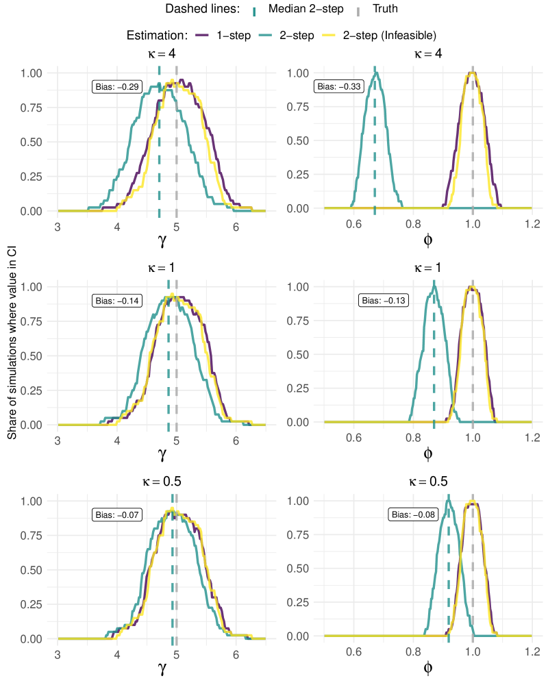
Note: Each mountain plot presents the share of simulations in which the value of (respectively ) on the -axis is included in the 95% confidence interval. The grey vertical dashed lines show the true value of the parameter. The blue vertical dashed line represents the median (across simulations) of mean posterior estimates from the two-step strategy. The bias reported is the difference between the truth and this median value.
Figure 1 presents the results. Each panel shows the coverage rates of confidence intervals for different parameter values: the share of simulations in which the values of the parameters are included in the 95% confidence intervals. The grey vertical dashed lines show the true value of the parameter. The blue vertical dashed line represents the median (across simulations) of mean posterior estimates for the two-step strategy. The two top panels show the results for the set of simulations where the amount of unstructured data per observation is the smallest and so is relatively large. The theory in Section 3 suggest that in this case we should expect the two-step strategy to perform badly. This is indeed the case. The median (across simulations) estimate of in top left, and in top right, are both substantially biased towards zero. Further, as predicted by theory, the width of the CIs using the two-step strategy is similar to the infeasible estimator that uses the true . This, together with the bias, means that the CIs based on the two-step strategy under-cover. For the true value is included in the 95% CI in only 32/40 (80%) of simulations. For this looks even worse: the true value is never included in the CIs.
On the other hand, the one-step strategy performs well. The estimates appear unbiased, and the CIs have close to expected coverage. The coverage is 92.5% for and 100% for . The difference from 95% is expected given the relatively low number of simulations we performed (40 per configuration). The difference between the lengths of CIs using the one-step strategy and those using the infeasible estimator is small but noticeable. In the former, is recognized as latent and the uncertainty in is accounted for when performing inference on and . The resulting CIs are approximately 10% wider than those obtained with the infeasible estimator that uses the true .
Moving down from the top panels, we can see the evolution of bias and coverage as the amount of unstructured data per observation increases and decreases. As predicted by theory, the bias in the two-step strategy becomes smaller as decreases. Increasing from 20 in the top panels to 80 in the middle reduces the absolute value of median bias in the two-step estimate of by about half, while the width of a typical CI virtually does not change, resulting in a large increase in CI coverage. A similar pattern is observed for . Meanwhile, the one-step strategy continues to perform well and one-step CIs are now indistinguishable from (infeasible) CIs based on the true . Finally, in the bottom panels, where and , the pattern continues. The bias in the two-step strategy is now very small for , though still noticeable for .
Overall, the simulations confirm the three main insights from Theorem 2: (1) there is a first order bias in the two-step strategy, which is driven by the mis-measurement of ; (2) the bias is larger when is larger; (3) the width of the confidence intervals is not substantially affected by mis-measurement of . The simulations also show that the one-step strategy performs well, and so it is a viable alternative to the two-step strategy. The one-step strategy is not only theoretically sound, but also leads to substantially less biased inference in practice.
Finally, a word on the computational performance is in order. We have found that Numpyro’s HMC implementation of the STMC model is fast—each simulation took approximately 4 minutes when estimated on a single mid-range professional GPU, the Nvidia V100. As such, we think that the one-step strategy is feasible for most researchers, and that the computational cost is not a major concern.
5.2 CEO Behavior
To show that modeling joint dependence and estimating jointly matters in practice, we revisit the study of Bandiera et al., (2020), which collects and analyzes data on CEO time use in a sample of manufacturing firms in several countries. The goal of that paper is to describe salient differences in executive time use, and to relate those differences to firm and CEO characteristics as well as firm outcomes.
The estimation sample consists of 916 CEOs, each of whom participated in a survey that recorded features of time use in each 15-minute interval of a given week, e.g. Monday 8am-8:15am, Monday 8:15am-8:30am, and so forth. The recorded categories are (1) the type of activity (meeting, public event, etc.); (2) duration of activity (15m, 30m, etc.); (3) whether the activity is planned or unplanned; (4) the number of participants in the activity; (5) the functions of the participants in the activity (HR, finance, suppliers, etc.). In total there are 654 unique combinations of these categories observed in the data. We let denote the number of times feature appears in the time use diary of CEO . The average value of is 88.4, with a minimum of 2 and a maximum of 222. Bandiera et al., (2020) uses LDA with dimensions to organize the time use data. The authors refer to the separate distributions over time use combinations and as pure behaviors. The share of CEO ’s time devoted to pure behavior , , is referred to as the CEO index.
The authors use the following inference procedure. First, estimate LDA on the time use data using the collapsed Gibbs sampler of Griffiths and Steyvers, (2004), then form an estimate based on the posterior means. They then use as an input into productivity regressions where is the log of firm sales, and is a vector of firm observables. Further, they separately analyzed which CEO and firm characteristics are associated with behaviors by regressing on a vector of characteristics .
We re-examine these questions using the Supervised Topic Model with Covariates. To explain CEO behavior, in we include log employment (a measure of firm size) and an indicator for whether the CEO has an MBA degree. To explain sales, in we include log employment and fixed effects for year and country. As before, we use HMC for inference and the same priors for both stratgies.202020We impose the anchor word assumption by zeroing out from () the activity that is relatively least likely in Pure Behavior 1 (2). The priors used are the same as in the simulation exercise, except that we set the Dirichlet concentration parameter to follow the original paper.
As demonstrated both theoretically and through the simulation exercise, the key quantity that governs the relative importance of sampling error and measurement error is . In the context of the CEO behavior data, the empirical analog of is the product of the square root of the number of observations (CEOs) and the average value of the inverse of the number of activities per CEO. This value is 0.44, which is close to the lowest value of in the simulation exercise. This suggests that the two-step approach should perform relatively well in this application. To further test our theory, we also estimate the model using data where we first sample 10% of the activities for each CEO, without replacement. This scenario could represent a researcher observing only half of a workday for each CEO, instead of a full five-day workweek. Such sampling increases the analogue of to 4.26, which is near the highest value of in the simulation exercise, indicating that we should expect the two-step approach to perform poorly under these conditions.
| Activity | 1-step | 2-step | Bandiera et al (2020) |
|---|---|---|---|
| Plant Visits | 0.1 | 0.09 | 0.11 |
| Suppliers | 0.41 | 0.44 | 0.32 |
| Production | 0.41 | 0.32 | 0.46 |
| Just Outsiders | 0.72 | 1.37 | 0.58 |
| Communication | 1.54 | 1.15 | 1.49 |
| Multi-Function | 1.4 | 1.17 | 1.9 |
| Insiders and Outsiders | 1.9 | 1.67 | 1.9 |
| C-suite | 21.57 | 13.01 | 33.9 |
-
•
Note: This table reports the relative probability of observing certain activities in Pure Behavior 1 relative to Pure Behavior 2. The value of 1 indicates that this activity is equally likely under both Pure Behaviors. Values higher than 1 mean that this type of activity is more likely to be performed under Pure Behavior 1. The values are reported in columns (1) and (2) are computed by first obtaining mean posterior probabilities of each activity in the given types. In column (3) we present values reported in Bandiera et al., (2020).
Turning to results, in Table 1 we report the relative probability of observing certain activities in Pure Behavior 1 relative to Pure Behavior 2. The table shows that estimated pure behaviors obtained with one-step and two-step strategies are very similar. What is more, they are also similar to those obtained with LDA and reported in the original paper. The table suggests that interacting with C-Suite executives, spending time communicating, and holding multi-function meetings are much more likely under Pure Behavior 1. Conversely, spending time on plant visits and interacting solely with suppliers are more likely under Pure Behavior 2. Based on these observations, the original authors label the CEOs with high values of as leaders and those with low values as managers.
Dependent variable: Log(sales) (1) 2-Step (2) 1-Step (3) 2-Step (4) 1-Step CEO Index 0.4 0.402 0.211 0.439 (0.219, 0.572) (0.240, 0.603) (-0.028, 0.449) (0.153, 0.711) Log Employment 1.212 1.198 1.239 1.199 (1.159, 1.268) (1.154, 1.248) (1.186, 1.29) (1.148, 1.26) Controls X X X X Activities’ Sample Full Full 10% 10%
Dependent variable: Un-normalized CEO index (1) 2-Step (2) 1-Step (3) 2-Step (4) 1-Step MBA 0.307 0.606 0.118 0.323 (0.176, 0.437) (0.446, 0.743) (-0.012, 0.249) (0.107, 0.486) Log Employment 0.356 0.492 0.154 0.443 (0.306, 0.406) (0.432, 0.548) (0.104, 0.204) (0.376, 0.507) Controls X X X X Activities’ Sample Full Full 10% 10%
Note: In parentheses we report symmetric (equal-tailed) 95% confidence interval.
In terms of the regression coefficient estimates, we find patterns that are consistent with theory and the simulation results. In Table 2, we report the estimates of the regression coefficients under the two-step and one-step strategies. In Panel (a), we show the estimates for the downstream coefficient , and in Panel (b), we show the estimates for the upstream coefficients . In both panels, columns (1) and (2) report the estimates obtained using one- and two-step strategies, respectively, for the full sample. The coefficient on the CEO index in the downstream model is equal to 0.4 and 0.402, respectively, in the two strategies; the CIs have a similar length and exclude 0. Thus, both strategies suggest that a larger share of time spent on Pure Behavior 1 is associated with higher firm productivity. In the upstream model, we see larger differences between the two strategies as in the simulations. While having an MBA and managing larger firms are both associated with a higher CEO index, the point estimates differ substantially. As suggested in the simulations, there appears to be a downward bias in the two-step strategy: for instance, the coefficient on the MBA dummy is equal to 0.307 in the two-step strategy, compared to 0.606 in the one-step strategy. The CIs are marginally wider in the one-step strategy (0.297 vs. 0.261), but as the theory predicts, the difference is not substantial. Note there is no overlap in the CIs for these coefficients: the one-step CIs lie entirely to the right of the two-step CIs.
The differences between the strategies are substantially more pronounced when we consider the estimates obtained using the 10% subsample of unstructured data. Under the one-step strategy, the empirical conclusions are largely the same as when using the full data. For example, the point estimate on changes from 0.402 to 0.439. While the confidence intervals are 54% wider than when using the full data (reflecting the increased uncertainty in estimated ), there is still a strong estimated relationship between CEO behavior and firm performance. This is not so with the two-step strategy: the point estimate of is now halved to 0.211, and the CI includes 0. Likewise, in the upstream model, the estimate of the coefficient on the MBA indicator remains large and statistically significant in the one-step strategy, but is reduced by 62% and is no longer statistically significant in the two-step strategy. This is consistent with the theory and simulation results, which suggest that the two-step strategy should perform particularly poorly in this scenario.
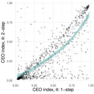
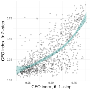
Note: Each point represents the mean posterior estimate of a single CEO’s index, . The blue line is the local polynomial fit (with confidence intervals) obtained with ‘ggplots’s’ ‘geom_smooth’ with default parameters.
What explains the differences in estimates across stratgies? To answer this question, we plot the estimated CEO indices in Figure 2. Panel (a) plots the estimated CEO indices obtained using the full sample, while Panel (b) plots the estimated CEO indices obtained using the 10% subsample. The blue line represents the local polynomial fit (with confidence intervals). The figure shows that when the full sample is used, both strategies find a large number of CEOs with close to 0 and 1, and a strong correlation between the two estimates. However, the correlation is much weaker for the 10% subsample, suggesting that there is a large scope for mis-measurement of . Interestingly, Proposition 2 suggests that the bias in the two-step estimate of can be severe when has mass near 0 and 1, as appears to be the case in this dataset. This provides an explanation for why the two-step strategy produces smaller estimates of even in the full dataset.
Taken together, both the simulation results and the analysis of CEO behavior data highlight the importance of having a large amount of unstructured data per observation. Without it, the coefficients estimated using the two-step strategy can be badly biased, which can lead to incorrect empirical conclusions. The good statistical and computational performance of the one-step strategy makes it attractive to guard against this risk.
6 Conclusion
The leading strategy for analyzing unstructured data uses two steps. First, quantitative representations of unstructured data are extracted in an information retrieval step. Second, the derived quantitative representations are plugged into downstream econometric models, with the representations treated as regular numerical data for the purposes of estimation and inference. This paper highlights, both theoretically and empirically, a previously unrecognized problem with this popular two-step strategy: measurement error introduced in the first step leads to biased estimates and invalid inference for downstream regression coefficients. The degree of bias, and therefore the degree to which it distorts inference, depends on the relative importance of measurement error and sampling error, but it can be material in applications. To guard against it, we propose a robust inference method based on maximum likelihood estimation of the information retrieval and regression models jointly. We implement this one-step strategy using Hamiltonian Monte Carlo deployed on modern hardware. This strategy outperforms the two-step strategy in simulations and generates quantitatively important differences in a leading application.
While we develop theoretical arguments within a simple regression model, we posit the same effects will arise in more elaborate downstream econometric models. For example, an emerging line of research uses text-derived sentiment indices as inputs into forecasting models with a vector autoregressive or dynamic factor structure. Straightforward extensions of our theoretical arguments can be used to show how error in the indices will bias coefficient estimates and limit the effectiveness of these forecasting methods. More constructively, the one-step strategy can be used to enhance the performance of these forecasting methods. Likewise, the industrial organization literature is increasingly using embedded representations of firms and products to characterize market behavior and demand with structural models. Our one-step strategy can be used to mitigate bias introduced by measurement error in the embeddings in these and other cases where the downstream model has a likelihood formulation. Going forward, it is important to establish for which specific information retrieval methods and econometric models does measurement error most severely affect inference.
Finally, we note there are limits on the scalability of Hamiltonian Monte Carlo, even when fully optimized. When one confronts a vast amount of data, alternative approaches for approximating the joint distribution in the one-step strategy must be used. One popular choice in computer science is variational inference (VI; Jordan et al., 1998, Wainwright and Jordan, 2008) which has recently seen applications in economics (Bonhomme, 2021, Olenski and Sacher, 2022, Mele and Zhu, 2023).212121Recently, scalable extensions of HMC that are based on stochastic approximations of gradients have shown initial promise (Dang et al., 2019). From an implementation perspective, VI is no more complicated than HMC because it too can be formulated within probabilistic programming languages that rely on automatic differentiation (Hoffman et al., 2013).222222For an example, see https://num.pyro.ai/en/stable/tutorials/tbip.html which illustrates a VI implementation of the Text-Based Ideal Points model (Vafa et al., 2020). However, VI has fewer statistical guarantees than HMC. In ongoing work, we are studying how to best perform scalable inference in the one-step strategy with massive data.
References
- Adams et al., (2021) Adams, R. B., Ragunathan, V., and Tumarkin, R. (2021). Death by Committee? An Analysis of Corporate Board (Sub-) Committees. Journal of Financial Economics, forthcoming.
- Ahrens et al., (2021) Ahrens, M., Ashwin, J., Calliess, J.-P., and Nguyen, V. (2021). Bayesian Topic Regression for Causal Inference. In Proceedings of the 2021 Conference on Empirical Methods in Natural Language Processing, pages 8162–8188, Online and Punta Cana, Dominican Republic. Association for Computational Linguistics.
- Allon et al., (2023) Allon, G., Chen, D., Jiang, Z., and Zhang, D. (2023). Machine Learning and Prediction Errors in Causal Inference. SSRN Electronic Journal.
- Arora et al., (2012) Arora, S., Ge, R., Kannan, R., and Moitra, A. (2012). Computing a nonnegative matrix factorization – provably. In Proceedings of the Forty-Fourth Annual ACM Symposium on Theory of Computing, STOC ’12, pages 145–162, New York, NY, USA. Association for Computing Machinery.
- Arora et al., (2016) Arora, S., Li, Y., Liang, Y., Ma, T., and Risteski, A. (2016). A Latent Variable Model Approach to PMI-based Word Embeddings. Transactions of the Association for Computational Linguistics, 4:385–399.
- Ash and Hansen, (2023) Ash, E. and Hansen, S. (2023). Text Algorithms in Economics. Annual Review of Economics, 15(1):659–688.
- Bai and Ng, (2006) Bai, J. and Ng, S. (2006). Confidence Intervals for Diffusion Index Forecasts and Inference for Factor-Augmented Regressions. Econometrica, 74(4):1133–1150.
- Baker et al., (2016) Baker, S. R., Bloom, N., and Davis, S. J. (2016). Measuring Economic Policy Uncertainty*. The Quarterly Journal of Economics, 131(4):1593–1636.
- Bandiera et al., (2021) Bandiera, O., Fischer, G., Prat, A., and Ytsma, E. (2021). Do Women Respond Less to Performance Pay? Building Evidence from Multiple Experiments. American Economic Review: Insights, 3(4):435–454.
- Bandiera et al., (2020) Bandiera, O., Prat, A., Hansen, S., and Sadun, R. (2020). CEO Behavior and Firm Performance. Journal of Political Economy, 128(4):1325–1369.
- Bernanke et al., (2005) Bernanke, B. S., Boivin, J., and Eliasz, P. (2005). Measuring the Effects of Monetary Policy: A Factor-Augmented Vector Autoregressive (FAVAR) Approach. The Quarterly Journal of Economics, 120(1):387–422.
- Betancourt, (2018) Betancourt, M. (2018). A Conceptual Introduction to Hamiltonian Monte Carlo. arXiv:1701.02434 [stat].
- Bing et al., (2020) Bing, X., Bunea, F., and Wegkamp, M. (2020). Optimal estimation of sparse topic models. Journal of Machine Learning Research, 21:1–45.
- Bingham et al., (2018) Bingham, E., Chen, J. P., Jankowiak, M., Obermeyer, F., Pradhan, N., Karaletsos, T., Singh, R., Szerlip, P., Horsfall, P., and Goodman, N. D. (2018). Pyro: Deep Universal Probabilistic Programming. arXiv:1810.09538 [cs, stat].
- Blei and McAuliffe, (2010) Blei, D. M. and McAuliffe, J. D. (2010). Supervised Topic Models. arXiv:1003.0783 [stat].
- Blei et al., (2003) Blei, D. M., Ng, A. Y., and Jordan, M. I. (2003). Latent dirichlet allocation. The Journal of Machine Learning Research, 3(null):993–1022.
- Bonhomme, (2021) Bonhomme, S. (2021). Teams: Heterogeneity, Sorting, and Complementarity. SSRN Electronic Journal.
- Bradbury et al., (2018) Bradbury, J., Frostig, R., Hawkins, P., Johnson, M. J., Leary, C., Maclaurin, D., Necula, G., Paszke, A., VanderPlas, J., Wanderman-Milne, S., and Zhang, Q. (2018). JAX: Composable transformations of Python+NumPy programs.
- Bybee et al., (2020) Bybee, L., Kelly, B. T., Manela, A., and Xiu, D. (2020). The Structure of Economic News. Technical Report w26648, National Bureau of Economic Research.
- Carpenter et al., (2017) Carpenter, B., Gelman, A., Hoffman, M. D., Lee, D., Goodrich, B., Betancourt, M., Brubaker, M., Guo, J., Li, P., and Riddell, A. (2017). Stan: A Probabilistic Programming Language. Journal of Statistical Software, 76(1):1–32.
- Chen et al., (2018) Chen, X., Christensen, T. M., and Tamer, E. (2018). Monte Carlo Confidence Sets for Identified Sets. Econometrica, 86(6):1965–2018.
- Chesher, (1991) Chesher, A. (1991). The effect of measurement error. Biometrika, 78(3):451–462.
- Compiani et al., (2023) Compiani, G., Morozov, I., and Seiler, S. (2023). Demand Estimation with Text and Image Data. Technical Report 10695, CESifo.
- Dang et al., (2019) Dang, K.-D., Quiroz, M., Kohn, R., Tran, M.-N., and Villani, M. (2019). Hamiltonian Monte Carlo with Energy Conserving Subsampling. Journal of Machine Learning Research, 20(100):1–31.
- Dieng et al., (2020) Dieng, A. B., Ruiz, F. J. R., and Blei, D. M. (2020). Topic Modeling in Embedding Spaces. Transactions of the Association for Computational Linguistics, 8:439–453.
- Draca and Schwarz, (2021) Draca, M. and Schwarz, C. (2021). How Polarized are Citizens? Measuring Ideology from the Ground-Up. SSRN Scholarly Paper ID 3154431, Social Science Research Network, Rochester, NY.
- Einav et al., (2022) Einav, L., Finkelstein, A., and Mahoney, N. (2022). Producing Health: Measuring Value Added of Nursing Homes.
- Fong and Tyler, (2021) Fong, C. and Tyler, M. (2021). Machine Learning Predictions as Regression Covariates. Political Analysis, 29(4):467–484.
- Gabaix et al., (2023) Gabaix, X., Koijen, R. S. J., and Yogo, M. (2023). Asset Embeddings. SSRN Electronic Journal.
- Gennaro and Ash, (2022) Gennaro, G. and Ash, E. (2022). Emotion and Reason in Political Language. The Economic Journal, 132(643):1037–1059.
- (31) Gentzkow, M., Kelly, B., and Taddy, M. (2019a). Text as Data. Journal of Economic Literature, 57(3):535–574.
- (32) Gentzkow, M., Shapiro, J. M., and Taddy, M. (2019b). Measuring Group Differences in High-Dimensional Choices: Method and Application to Congressional Speech. Econometrica, 87(4):1307–1340.
- Gorodnichenko et al., (2023) Gorodnichenko, Y., Pham, T., and Talavera, O. (2023). The Voice of Monetary Policy. American Economic Review, 113(2):548–584.
- Griffiths and Steyvers, (2004) Griffiths, T. L. and Steyvers, M. (2004). Finding scientific topics. Proceedings of the National Academy of Sciences, 101(suppl 1):5228–5235.
- Hansen et al., (2018) Hansen, S., McMahon, M., and Prat, A. (2018). Transparency and Deliberation Within the FOMC: A Computational Linguistics Approach*. The Quarterly Journal of Economics, 133(2):801–870.
- Herbst and Schorfheide, (2016) Herbst, E. P. and Schorfheide, F. (2016). Bayesian Estimation of DSGE Models. Princeton University Press, Princeton.
- Hoberg and Phillips, (2016) Hoberg, G. and Phillips, G. (2016). Text-Based Network Industries and Endogenous Product Differentiation. Journal of Political Economy, 124(5):1423–1465.
- Hoffman et al., (2013) Hoffman, M. D., Blei, D. M., Wang, C., and Paisley, J. (2013). Stochastic Variational Inference. Journal of Machine Learning Research, 14(4):1303–1347.
- Hoffman and Gelman, (2014) Hoffman, M. D. and Gelman, A. (2014). The No-U-Turn Sampler: Adaptively Setting Path Lengths in Hamiltonian Monte Carlo. Journal of Machine Learning Research, 15(47):1593–1623.
- Hofmann, (1999) Hofmann, T. (1999). Probabilistic latent semantic indexing. In Proceedings of the 22nd Annual International ACM SIGIR Conference on Research and Development in Information Retrieval, pages 50–57, Berkeley California USA. ACM.
- Jordan et al., (1998) Jordan, M. I., Ghahramani, Z., Jaakkola, T. S., and Saul, L. K. (1998). An Introduction to Variational Methods for Graphical Models. In Jordan, M. I., editor, Learning in Graphical Models, NATO ASI Series, pages 105–161. Springer Netherlands, Dordrecht.
- Ke et al., (2021) Ke, S., Olea, J. L. M., and Nesbit, J. (2021). Robust Machine Learning Algorithms for Text Analysis. Unpublished manuscript.
- Ke and Wang, (2022) Ke, Z. T. and Wang, M. (2022). Using SVD for Topic Modeling. Journal of the American Statistical Association, pages 1–16.
- Kogan et al., (2019) Kogan, L., Papanikolaou, D., Schmidt, L., and Seegmiller, B. (2019). Technology, Vintage-Specific Human Capital, and Labor Displacement: Evidence from Linking Patents with Occupations.
- Larsen and Thorsrud, (2019) Larsen, V. H. and Thorsrud, L. A. (2019). The value of news for economic developments. Journal of Econometrics, 210(1):203–218.
- MacKay, (2003) MacKay, D. J. C. (2003). Information Theory, Inference and Learning Algorithms. Cambridge University Press, Cambridge, UK ; New York, illustrated edition edition.
- Magnolfi et al., (2022) Magnolfi, L., McClure, J., and Sorensen, A. (2022). Embeddings and Distance-based Demand for Differentiated Products. In Proceedings of the 23rd ACM Conference on Economics and Computation, EC ’22, page 607, New York, NY, USA. Association for Computing Machinery.
- Malmendier et al., (2021) Malmendier, U., Nagel, S., and Yan, Z. (2021). The making of hawks and doves. Journal of Monetary Economics, 117:19–42.
- Mardia et al., (2019) Mardia, J., Jiao, J., Tánczos, E., Nowak, R. D., and Weissman, T. (2019). Concentration Inequalities for the Empirical Distribution.
- Meager, (2019) Meager, R. (2019). Understanding the Average Impact of Microcredit Expansions: A Bayesian Hierarchical Analysis of Seven Randomized Experiments. American Economic Journal: Applied Economics, 11(1):57–91.
- Mele and Zhu, (2023) Mele, A. and Zhu, L. (2023). Approximate Variational Estimation for a Model of Network Formation. The Review of Economics and Statistics, 105(1):113–124.
- (52) Mikolov, T., Chen, K., Corrado, G., and Dean, J. (2013a). Efficient Estimation of Word Representations in Vector Space. arXiv:1301.3781 [cs].
- (53) Mikolov, T., Sutskever, I., Chen, K., Corrado, G., and Dean, J. (2013b). Distributed Representations of Words and Phrases and their Compositionality. arXiv:1310.4546 [cs, stat].
- Mueller and Rauh, (2018) Mueller, H. and Rauh, C. (2018). Reading Between the Lines: Prediction of Political Violence Using Newspaper Text. American Political Science Review, 112(2):358–375.
- Müller, (2013) Müller, U. (2013). Risk of Bayesian Inference in Misspecified Models, and the Sandwich Covariance Matrix. Econometrica, 81(5):1805–1849.
- Munro and Ng, (2022) Munro, E. and Ng, S. (2022). Latent Dirichlet Analysis of Categorical Survey Responses. Journal of Business & Economic Statistics, 40(1):256–271.
- Neal, (2012) Neal, R. M. (2012). MCMC using Hamiltonian dynamics. arXiv:1206.1901 [physics, stat].
- Nimczik, (2017) Nimczik, J. S. (2017). Job Mobility Networks and Endogenous Labor Markets. Technical Report 168147, Verein für Socialpolitik / German Economic Association.
- Olenski and Sacher, (2022) Olenski, A. and Sacher, S. (2022). Estimating Nursing Home Quality with Selection.
- Olivella et al., (2021) Olivella, S., Pratt, T., and Imai, K. (2021). Dynamic Stochastic Blockmodel Regression for Network Data: Application to International Militarized Conflicts. arXiv:2103.00702 [cs, stat].
- Pagan, (1984) Pagan, A. (1984). Econometric Issues in the Analysis of Regressions with Generated Regressors. International Economic Review, 25(1):221–247.
- Phan et al., (2019) Phan, D., Pradhan, N., and Jankowiak, M. (2019). Composable Effects for Flexible and Accelerated Probabilistic Programming in NumPyro. arXiv:1912.11554 [cs, stat].
- Phillips, (1987) Phillips, P. C. B. (1987). Towards a unified asymptotic theory for autoregression. Biometrika, 74(3):535–547.
- Roberts et al., (2014) Roberts, M. E., Stewart, B. M., Tingley, D., Lucas, C., Leder-Luis, J., Gadarian, S. K., Albertson, B., and Rand, D. G. (2014). Structural Topic Models for Open-Ended Survey Responses. American Journal of Political Science, 58(4):1064–1082.
- Ruiz et al., (2020) Ruiz, F. J. R., Athey, S., and Blei, D. M. (2020). SHOPPER: A probabilistic model of consumer choice with substitutes and complements. The Annals of Applied Statistics, 14(1):1–27.
- Staiger and Stock, (1997) Staiger, D. and Stock, J. H. (1997). Instrumental Variables Regression with Weak Instruments. Econometrica, 65(3):557–586.
- Stock and Watson, (2002) Stock, J. H. and Watson, M. W. (2002). Forecasting Using Principal Components from a Large Number of Predictors. Journal of the American Statistical Association, 97(460):1167–1179.
- Thorsrud, (2020) Thorsrud, L. A. (2020). Words are the New Numbers: A Newsy Coincident Index of the Business Cycle. Journal of Business & Economic Statistics, 38(2):393–409.
- Tropp, (2012) Tropp, J. A. (2012). User-Friendly Tail Bounds for Sums of Random Matrices. Foundations of Computational Mathematics, 12(4):389–434.
- Vafa et al., (2023) Vafa, K., Athey, S., and Blei, D. M. (2023). Decomposing Changes in the Gender Wage Gap over Worker Careers. In NBER Summer Institute, Boston, MA.
- Vafa et al., (2020) Vafa, K., Naidu, S., and Blei, D. (2020). Text-Based Ideal Points. In Jurafsky, D., Chai, J., Schluter, N., and Tetreault, J., editors, Proceedings of the 58th Annual Meeting of the Association for Computational Linguistics, pages 5345–5357, Online. Association for Computational Linguistics.
- van der Vaart, (1998) van der Vaart, A. W. (1998). Asymptotic Statistics. Cambridge University Press, Cambridge, UK.
- Wainwright and Jordan, (2008) Wainwright, M. J. and Jordan, M. I. (2008). Graphical Models, Exponential Families, and Variational Inference. Foundations and Trends® in Machine Learning, 1(1–2):1–305.
- White, (1980) White, H. (1980). A Heteroskedasticity-Consistent Covariance Matrix Estimator and a Direct Test for Heteroskedasticity. Econometrica, 48(4):817.
- Wu et al., (2023) Wu, R., Zhang, L., and Tony Cai, T. (2023). Sparse Topic Modeling: Computational Efficiency, Near-Optimal Algorithms, and Statistical Inference. Journal of the American Statistical Association, 118(543):1849–1861.
- Zhang et al., (2023) Zhang, J., Xue, W., Yu, Y., and Tan, Y. (2023). Debiasing Machine-Learning- or AI-Generated Regressors in Partial Linear Models. SSRN Electronic Journal.
Appendix A Proofs
Notation
Let denote the Euclidean norm when applied to vectors and the spectral norm when applied to matrices. Let denote the Frobenius norm.
A.1 Proofs for Section 2
Proof of Proposition 1.
We start by writing
where . Note by Chebyshev’s inequality that for integers and any , we have
Consider the denominator term in and . By Chebyshev’s inequality, we have
where, by the law of total variance and independence of and ,
because .
For the numerator in , we similarly have
Because and , we have
A second application of Chebyshev’s inequality gives
Hence,
For , we have
because . Note that because and are independent conditional on and both and have conditional (on ) mean zero. Hence by Chebyshev’s inequality, for any we have
because and are independent conditional on , and are independent, and . Finally, is asymptotically by the central limit theorem. ∎
The next assumption is used to derive Proposition 2.
Assumption 3.
-
(i)
, , and .
-
(ii)
for some .
-
(iii)
almost surely for some .
Part (i) is standard and ensures the OLS estimator of without measurement error is well defined with finite asymptotic variance. Part (ii) is made to simplify technical arguments and can be relaxed, e.g., by controlling the rate at which the distribution of behaves at the boundary of its support. Finally, part (iii) is the same as Assumption 2(v) and is also made to simplify technical derivations and can be relaxed.
Proof of Proposition 2.
To simplify notation, let and . We have
where . It follows by standard arguments that under Assumption 3(i), we have
and .
It remains to characterize the numerator of . To this end, first note that with as in Assumption 3(ii), we have
| (almost surely) | |||||
| (almost surely) | |||||
where the first inequality is by the union bound, the second is by Assumption 3(ii), the third is by Chernoff’s inequality for Binomial random variables, and the fourth is because for some and both hold for all with probability one by Assumptions 3(ii) and 3(iii). Therefore,
| (16) |
We may similarly deduce that
| (17) |
and that
| (18) |
In view of Assumption 3(ii), condition (18) also implies that because is uniformly continuous on . But then note that this implies
by Assumption 3(i). It therefore remains to show
By Taylor’s theorem, we have
where is between and . Note that Assumption 3(ii) implies that . We also have by (16) and (17) that with probability approaching one (wpa1). Thus, all terms on the right-hand side are well defined wpa1. We control the covariance of with these terms using and and the fact that and are independent conditional on as follows:
First, by Chebyshev’s inequality, we have for that
by (3), independence of and conditional on , and independence of and . Second, we similarly have
Moreover, letting and noting and because , we have by Chebyshev’s inequality that for ,
Finally, because holds for all wpa1, there is a positive constant such that
holds wpa1. Hence, in view of (18), it suffices to show that the right-hand side term is bounded in probability. To this end, note by Markov’s inequality that for ,
as required. ∎
A.2 Proofs for Section 3
The next two lemmas apply in both fixed-populations and sequences-of-populations.
Lemma 1.
Suppose that (5) holds and that and are independent. Then
In addition, if and and are independent conditional on , then
Proof of Lemma 1.
First note by (5) that
where the second-last line follows from the mean and variance of the multinomial distribution and the final line is by independence of and . For the second result, using conditional independence of and given , we have
as required. ∎
Proof of Lemma 2.
In view of Assumption 1(iii), we have
where exists with probability approaching one by Assumption 1(ii) and because has full rank. Each element of is bounded between and , so we may deduce by Chebyshev’s inequality that
Hence by Assumption 1(ii) and Slutsky’s theorem, we have
The result follows by Lemma 1. ∎
Proof of Theorem 1.
First consider the denominator. By Lemma 2, we have
| (19) |
For the numerator term, again by Assumption 1(iii), we have
where by the LLN and Lemma 1, we have
It follows by Assumption 1(ii) and Slutsky’s theorem that
| (20) |
The first result follows from (19) and (20). Note that the matrix on the right-hand side of (19) is bounded below (in Loewner order) by so its inverse is well defined by Assumption 1(i). The second result follows from the approximation for invertible and small. ∎
Proof of Theorem 2.
First consider the denominator term. By Lemma 2 and condition (7), we have . Hence, by Assumption 2(i),
| (21) |
Now consider the numerator term. We first write
Consider term . By Assumption 2(iii), we have
where
Assumptions 2(i) and 2(ii) together imply that , from which it follows that . For term note that
| (22) |
Let . Then
where the second inequality is because is in the simplex and the third inequality is by (22). Hence it follows by Chebyshev’s inequality that
and so
Finally, by (7), (22), and Assumption 2(ii) we conclude that
| (23) |
Now consider term . Again by Assumption 2(i)-(iii), we have
Consider the sum in parentheses. The summands have mean zero (by (4)) and variance
| (24) |
In the above derivation, the first equality uses conditional independence of and given , the second uses independence of and and the fact that is multinomial, the third uses independence of and . Finally, in view of (7), we obtain
Note the right-hand side matrix has full rank by Assumption 2(i). Moreover, as takes values in the simplex, we have . Hence, for all ,
by Assumption 2(iv). It follows by the Lindeberg–Feller central limit theorem that
| (25) |
For result (9), it remains to show
To this end, first note that in view of Assumption 2(iii) we have
Write
First consider term . By (24) we have
Moreover, for any positive constant we can write
where and . For term , note that the summands have mean zero, satisfy
and
because . Applying Theorem 1.4 of Tropp, (2012), for any we have
provided as . For , we have
as by Assumption 2(iv). In particular, choosing ensures that both and are asymptotically negligible in which case and so
Now consider . As , we have
But note that , where
by Assumption 2(iii), consistency of , and the fact that is bounded in probability by Assumptions 2(i) and 2(ii). Moreover,
where by Assumptions 2(i) and 2(ii). Further, as , for all we have
by the union bound and Lemma 1 of Mardia et al., (2019). Hence by Assumption 2(v), we have
for . Hence, and so . It follows that by Hölder’s inequality. Hence, by Assumptions 2(i) and 2(ii) we conclude that . ∎
Appendix B Further Details on the Simulation Exercise
Table B.1 presents the parameters used for simulation exercise. Since we used types and type shares must add to 1, only the differences in regression parameters, e.g. are identified, therefore in the simulation and estimation we normalized and to 0. Second, since class ‘labels’ are not identified in estimation, it is necessary to adjust signs post estimation.
To investigate the impact of on the estimation of , we ran three sets of simulations which vary only by the total number of features drawn per observations. For simplicity, in each of the set of simulations we set to be equal for all . We set which, given that is fixed to 6400 corresponds to .
To ensure the model is properly identified, in each simulation we set features to be ‘anchor words’ meaning that or is set to 0.
We simulated data 40 times for each set and then estimated the model using 1-step approach, 2-step approach and the infeasible 2-step approach with known .
We construct 95% confidence intervals for and using the corresponding 95% posterior credible intervals for these parameters. This construction is justified in view of the discussion in Section 4.2.
Parameter Value Description (a) Data Simulation Number of observations Number of distinct features Total number of features per document Number of latent types True 1 Effect of a covariates on un-normalized type shares True 5 Effect of topic shares on numerical outcomes True Effect of additional covariates on numerical outcomes Covariate affecting type shares Additional covariates affecting outcome SD of the numeric outcome’s residual SD of residual of the un-normalized type shares Dirichlet concentration parameter (a) Hyperparameters as above Number of latent types as above Dirichlet concentration parameter as above SD of residual of the un-normalized type shares Prior for , i.e. Prior for , i.e. Prior for , i.e. Prior for , i.e. and
We performed the simulation on a ‘N1-highmem-2’ instance on the Google Could Platform. The instance has 2 vCPUs and 13 GB of memory. We also utilized a single Tesla V100 GPU. We run chose 2000 warmup ans 2000 post-warmup iterations. A single simulation (consisting of drawing the data, and estimating the model in three ways) took approximately 10 minutes.