Fireball anti-nucleosynthesis

Abstract

The tentative identification of approximately ten relativistic anti-helium ($\overline{\text{He}}$) cosmic-ray events at AMS-02 would, if confirmed, challenge our understanding of the astrophysical synthesis of heavy anti-nuclei. We propose a novel scenario for the enhanced production of such anti-nuclei that is triggered by isolated, catastrophic injections of large quantities of energetic Standard Model (SM) anti-quarks in our galaxy by physics beyond the Standard Model (BSM). We demonstrate that SM anti-nucleosynthetic processes that occur in the resulting rapidly expanding, thermalized fireballs of SM plasma can, for a reasonable range of parameters, produce the reported tentative $\sim 2:1$ ratio of ${}^{3}\overline{\text{He}}$ to ${}^{4}\overline{\text{He}}$ events at AMS-02, as well as their relativistic boosts. Moreover, we show that this can be achieved without violating anti-deuterium or anti-proton flux constraints for the appropriate anti-helium fluxes. A plausible BSM paradigm for the catastrophic injections is the collision of macroscopic composite dark-matter objects carrying large net anti-baryon number. Such a scenario would require these objects to be cosmologically stable, but to destabilize upon collision, promptly releasing a fraction of their mass energy into SM anti-particles within a tiny volume. We show that, in principle, the injection rate needed to attain the necessary anti-helium fluxes and the energetic conditions required to seed the fireballs appear possible to obtain in such a paradigm. We leave open the question of constructing a BSM particle physics model to realize this, but we suggest two concrete scenarios as promising targets for further investigation.

I Introduction

The AMS-02 Collaboration has unofficially reported [2, 3, 4, 5, 6, 7] $\mathcal{O}(10)$ highly relativistic cosmic-ray events detected in $\sim 10$ years of data that are consistent with tentative identification as anti-helium [6, 7]. Although publicly available mass determinations are uncertain [6], the data are reported to be consistent with tentative identification of both ${}^{3}\overline{\text{He}}$ and ${}^{4}\overline{\text{He}}$ candidate events, with an event ratio of roughly $N_{{}^{3}\overline{\text{He}}}:N_{{}^{4}\overline{\text{He}}}\sim 2:1$ (albeit with small statistics and large uncertainties) [6, 7]. Additionally, tentative identification of 7 anti-deuterium candidate events has recently been reported [7].

While the tentative identifications of these candidate events require more work to confirm [7], the anti-helium candidates in particular have been the subject of extensive recent interest in the literature [8, 9, 10, 11, 12, 13, 14, 15, 16, 17, 18] because, taken at face-value, they are surprising: the formation of complex anti-nuclei in astrophysical environments is challenging and the rates of production implied by these candidate events are hard to reconcile with known Standard Model (SM) physics.

Within the SM, a known source of anti-nucleus cosmic rays is spallation induced by primary cosmic rays (hydrogen or helium) in the interstellar medium (ISM) [12]. Spallation is, however, inefficient at producing anti-nuclei; due to kinematics, this is particularly true for those anti-nuclei with higher atomic mass number $A$, such as ${}^{4}\overline{\text{He}}$. Coalescence of two anti-nucleons or anti-nuclei (or of an anti-nucleon and an anti-nucleus) produced in spallation into a higher-$A$ anti-nucleus is probable only if their relative kinetic energy is comparable to or below the difference in the nuclear binding energies $E_{B}$ of the initial and final states; roughly, $E_{B}\sim A\times\mathcal{O}(\mathinner{\mathrm{MeV}})$. On the other hand, the threshold energy for production of nuclear anti-particles via spallation of a primary cosmic ray against the ISM is $E_{\text{th}}\sim m_{\bar{N}}\sim A\mu_{a}\sim A\times\mathcal{O}(\mathinner{\mathrm{GeV}})$. Because primary cosmic-ray fluxes tend to be power laws as a function of energy (see, e.g., Ref. [1]), it follows that the kinetic energy of nuclear anti-particles produced by spallation of sufficiently energetic primary cosmic rays is also of typically $\mathcal{O}(\text{GeV})$, except very near threshold. The formation rates of heavier anti-nuclei via coalescence of such products therefore tend to suffer significant phase-space suppressions, leading to strong hierarchies between the expected numbers $N$ of anti-nucleus events with subsequently higher $A$ that would be observed at AMS-02: i.e., $N_{\bar{p}}\gg N_{{\mkern-2.0mu\bar{\mkern 2.0mu\text{D}}}}\gg N_{{}^{3}\overline{\text{He}}}\gg N_{{}^{4}\overline{\text{He}}}$.

These conventional astrophysics predictions for anti-nucleus cosmic ray fluxes from spallation were quantified recently in Ref. [12], where the expected numbers of anti-nucleus events at AMS-02 were found to scale roughly as $N_{\bar{p}}\sim 10^{4}N_{{\mkern-2.0mu\bar{\mkern 2.0mu\text{D}}}}\sim 10^{8}N_{{}^{3}\overline{\text{He}}}\sim 10^{12}N_{{}^{4}\overline{\text{He}}}$, in line with the phase-space argument above. For model parameters that reproduce the anti-proton flux observed by AMS-02, Ref. [12] thus found that the predicted anti-helium fluxes are always orders of magnitude below AMS-02 sensitivity. Conversely, in order to reproduce, e.g., the tentatively identified ${}^{4}\overline{\text{He}}$ flux, one would have to overproduce, e.g., the observed anti-proton flux by many orders of magnitude.

Similar challenges in producing anti-nuclei also occur in decaying or annihilating particle dark-matter models commonly studied in the context of indirect searches [12, 10, 11, 8, 9]. The anti-nucleus production rates in these models suffer from similar phase-space suppressions for spallation of primary cosmic rays. One should keep in mind however that there are considerable variations in the predicted anti-nucleus fluxes stemming from uncertainties in the parameters of the nuclear-coalescence model [8, 9] and different choices of the cosmic-ray propagation model [14]. With optimistic assumptions [14, 11], and possibly with enhancements from $\overline{\Lambda_{b}}$ decays [15], it has been found that it might be possible for annihilating particle dark matter to be the origin of the tentatively identified ${}^{3}\overline{\text{He}}$ flux. However, even a single confirmed ${}^{4}\overline{\text{He}}$ event at AMS-02 would be challenging to explain.

If the candidate events are confirmed, explaining the presence of both the ${}^{3}\overline{\text{He}}$ and ${}^{4}\overline{\text{He}}$ events at AMS-02, with their comparable rates, seems to require the absence of the severe phase-space suppressions that inexorably lead to a strong hierarchical relation of the anti-nucleus fluxes. These suppressions can be ameliorated if the anti-nucleons that combined to form the anti-nuclei have low relative momenta, $\Delta p\ll\mathinner{\mathrm{GeV}}$. Various beyond-the-Standard-Model (BSM) scenarios have been proposed to achieve this.

Refs. [12, 16, 18] considered anti-nucleus production occurring in anti-matter–dominated regions of primordial origin that have cooled down significantly by the time of the anti-nucleus production. These scenarios require a BSM mechanism in the early Universe to cause the requisite matter–anti-matter segregation.

Anti-nucleus production scenarios via the decay of a new particle carrying anti-baryon number (which may or may not be the dark matter) have been also considered. In Ref. [13], the mass of the decaying particle was tuned to be very close to the mass of the desired anti-nucleus in order to restrict the final-state phase space, such that the produced particles are non-relativistic. Such a scenario however requires several new decaying particles, each with its own mass tuning to separately enhance the production of ${}^{4}\overline{\text{He}}$, ${}^{3}\overline{\text{He}}$, and perhaps ${\mkern-2.0mu\bar{\mkern 2.0mu\text{D}}}$. In Ref. [17], a strongly coupled dark sector was considered, where dark hadron showers triggered by the decay of a new particle simultaneously increase the multiplicity of the decay products and decrease their relative momenta $\Delta p$. The final decay products (i.e., the lightest dark bound states) then decay to SM anti-quarks which subsequently form anti-nuclei. A challenging aspect of this scenario is the need to model strong-coupling phenomena such as dark hadron showers.

Another challenging aspect of the tentatively identified events at AMS-02 is their relativistic nature (i.e., large Lorentz boosts). Overcoming phase-space suppressions of nuclear coalescence rates by considering scenarios where the colliding particles have low relative momenta usually also results in anti-helium products that are non-relativistic. There are however ways around this: the anti-helium products in scenarios that start with the decay of a particle, such as those considered in Refs. [13, 17], can be made relativistic if the decaying particle is already boosted in the galactic rest frame. This can be achieved if, e.g., the decaying particle is produced in turn from the earlier decay of another heavier particle. Other works [12, 16, 18] have either suggested acceleration mechanisms based on supernova shockwaves (similar to the Fermi mechanism), or did not address this question.

In this paper, we propose a scenario where the anti-helium nuclei observed at AMS-02 originate from sudden and localized “injections” (of BSM origin) of anti-baryon number in our Galaxy in the form of energetic SM anti-quarks. These particles subsequently thermalize into relativistically expanding, optically thick fireballs with a net anti-baryon number. Anti-nuclei are produced in each of these fireballs thermally through a nuclear reaction chain similar to that operating during Big Bang Nucleosynthesis (BBN), albeit with remarkable qualitative and quantitative differences due to the very different (anti-)baryon–to–entropy ratios, timescales, and expansion dynamics involved. The evolution of the fireball plasma after the initial injection of SM particles is purely dictated by SM physics and, moreover, since this process involves thermalization, depends only on certain bulk properties being achieved by the injection, and for the most part not on the exact details of the latter. However, owing to the inefficiency of weak interactions, there are regions of parameter space where the anti-neutron–to–anti-proton ratio in the plasma at the onset of the anti-nucleosynthetic processes may depend on the details of the initial injection of SM particles. With that one exception, the predicted anti-particle cosmic ray fluxes produced in our proposed scenario are therefore both predictive and largely agnostic as to the microphysical origin of the injections that seed these fireballs.

Assuming that the requisite injections can occur, we show that this scenario could explain not only the tentatively identified anti-nucleus fluxes at AMS-02, but also the relativistic Lorentz boosts of the detected particles. The seemingly paradoxical requirements of a low-energy environment to foster production of higher-$A$ anti-nuclei and the high energies required for relativistic anti-nucleus products are reconciled naturally in our scenario by the expansion dynamics of the fireball plasma: as the plasma expands, its temperature falls adiabatically while its thermal energy is converted to bulk kinetic energy by the work of its internal pressure. This allows a low-energy environment for anti-nucleosynthesis to proceed, while at the same time accelerating its products to relativistic speeds.

Of course, injections of the requisite amounts of SM anti-particles with the correct properties to generate these fireballs cannot occur spontaneously: a BSM mechanism is required. Suggestively, we show that collisions of certain very heavy, macroscopic, composite dark objects (possibly a sub-fraction of all of the dark matter) that carry SM anti-baryon number could at least achieve a high-enough rate of injections with appropriate parameters to explain the tentatively identified anti-helium events at AMS-02, provided that a substantial fraction of the dark objects’ mass energy can be converted into SM anti-quarks as a result of dark-sector dynamics triggered by the collision (in some parameter regions, there may be a requirement to inject also a comparably sized asymmetry of charged leptons). While this is encouraging, we have not yet developed a detailed microphysical model that achieves the necessary dark-sector dynamics in a way that is amenable to robust and controlled understanding; however, we offer some speculative initial thoughts on certain model constructions that we believe are promising avenues to explore toward that goal. For the purposes of this paper, we ultimately leave this question open; as it is crucial to providing a concrete realization of the scenario we advance, however, we both intend to return to it in our own future work and we encourage other work on it.

The remainder of this paper is structured as follows. In Sec. II, we review the candidate anti-nuclei events observed by AMS-02. In Sec. III, we discuss synthesis of anti-nuclei in an expanding relativistic fireball, discussing first questions of thermalization after energy injection [Sec. III.1], then turning to the fireball expansion dynamics [Sec. III.2], and the nuclear reactions at play [Sec. III.3], before summarizing [Sec. III.4]. In Sec. IV, we then discuss how the anti-nuclei thus produced would propagate to AMS-02 and give our scenario’s projections for the anti-nuclei spectra and event rates [Sec. IV.1]; we also discuss other potential observables [Sec. IV.2]. In Sec. V, we discuss a potential origin for the fireballs in collisions of composite dark-matter states, showing first that the rates could work [Sec. V.1], that the fireballs could be appropriately seeded if certain benchmarks can be met [Sec. V.2], and then offering some speculative thoughts toward particle physics models that may be worth further investigation to see it they are able to achieve the necessary conditions [Sec. V.3]. We conclude in Sec. VI. A number of appendices add relevant detail. Appendix A gives derivations of various scaling laws for fireball expansion that we rely on in the main text. Appendix B discusses the ratio of anti-nucleons from which the anti-nucleosynthesis is initiated. Appendices C and D, respectively, give details of the nuclear reaction networks and cross-sections we have used. Appendix E discusses whether dynamical changes in the number of degrees of freedom during fireball expansion are relevant. Appendix F discusses prompt versus slow injections. Finally, Appendix G reviews an estimate of the AMS-02 rigidity-dependent sensitivity to anti-helium events.

II The AMS-02 candidate anti-helium events

In this section, we summarize the data that is publicly available [2, 3, 4, 5, 6, 7] regarding the AMS-02 candidate anti-helium and anti-deuterium events.

#	Event Date [mm/dd/yyyy] (Day of Year)	$p$ [GeV]	$m$ [GeV]	$Q/e$	$\Gamma$	$\mathcal{R}$ [GV]	Ref(s).
1	09/26/2011 (269)	$33.1(1.6)$	$2.93(36)$	$-1.97(5)$	$11.3(1.5)$	$-16.80(92)$	[3, 4]
2	12/08/2016 (—)	$40.3(2.9)$	$2.96(33)$	$-2$(—)	$13.6(1.3)$	$-20.2(1.5)$	[2, 3]
3	06/22/2017 (173)	$32.6(2.5)$	$3.81(29)$	$-2.05(5)$	$8.61(92)$	$-15.9(1.3)$	[3, 5, 7]
4	09/20/2022 (265)	—	$3.15(53)$	$-2$	—	—	[7]

Table 1: Parameters for individual candidate anti-helium events displayed in the identified references: $p$ is momentum, $m$ is mass, $Q$ is charge ($e>0$ is the elementary charge), $\Gamma$ is the Lorentz factor, and $\mathcal{R}=p/Q$ is rigidity. For identification purposes across the references, the reported event date and corresponding day of year are given (the date of event 2 is not given in the references; we give the date of its first public presentation in Ref. [2]). Unavailable data are denoted by “—”. We have set $\hbar=c=1$. Data for $p$, $m$, and $Q/e$ are given in the references [speed data, $v=0.9973(5)$, is additionally given for event 2]; we derived $\Gamma=\sqrt{1+(p/m)^{2}}$ [or $\Gamma=1/\sqrt{1-v^{2}}$ for event 2] and $\mathcal{R}=p/Q$ and propagated uncertainties naïvely. For comparison, $m_{{}^{3}\overline{\text{He}}}=2.81\,\mathinner{\mathrm{GeV}}$ and $m_{{}^{4}\overline{\text{He}}}=3.73\,\mathinner{\mathrm{GeV}}$. Event # 3 is clearly tentatively identified in Refs. [3, 7] as a candidate ${}^{4}\overline{\text{He}}$ event. Event # 4, which is similarly identified as an ${}^{4}\overline{\text{He}}$ candidate in the oral presentation of Ref. [7], is not included in our analysis; see discussion in text.

To our knowledge, the most recent scientific presentations on these candidate events are Refs. [6, 7]. Ref. [6] provides graphical mass and rigidity histogram data for 9 candidate events collected in $\sim 10\ \text{years}$ of AMS-02 observations. Ref. [7] also appears to show an additional anti-helium candidate event dated after Ref. [6], with a mass measurement consistent with either ${}^{3}\overline{\text{He}}$ or ${}^{4}\overline{\text{He}}$, but closer to the former. Table 1 shows the detailed basic parameter values for 3 of the 9 candidate events that have been shown publicly [2, 3, 4, 5, 7], as well as the data available for the additional candidate event [7]; such detailed data has not been presented for the other candidate events.

We base our analysis on the data for the 9 candidate events presented in Ref. [6], which are consistent with the identification of 6 candidate ${}^{3}\overline{\text{He}}$ events, and 3 candidate ${}^{4}\overline{\text{He}}$ events in $T\sim 10\,\text{years}$ of AMS-02 data (see discussion about $T$ below).^, The mass histogram shown in Ref. [6] is however more than broad enough to support an inference that some of the candidate ${}^{3}\overline{\text{He}}$ events thus classified could in fact be ${}^{4}\overline{\text{He}}$ events, and vice versa (the additional event shown in Ref. [7] could also be identified as either isotope within the uncertainties). Nevertheless, throughout this paper, we adopt a $\sim 2:1$ event ratio for ${}^{3}\overline{\text{He}}$ vs. ${}^{4}\overline{\text{He}}$ as fiducial.

Of the candidate events in Ref. [6], 3 have rigidities $\mathcal{R}=p/Q$ (where $p$ is the particle momentum and $Q=qe$ its charge) in the approximate range $-40\,\text{GV}\lesssim\mathcal{R}\lesssim-35\,\text{GV}$, while the other 6 candidate events have rigidities in the range $-25\,\text{GV}\lesssim\mathcal{R}\lesssim-15\,\text{GV}$. The data in Table 1 however make clear that care should be taken not to associate the 3 candidate events with larger $|\mathcal{R}|$ shown in the histogram in Ref. [6] with the 3 candidate ${}^{4}\overline{\text{He}}$ events and the remainder with the 6 candidate ${}^{3}\overline{\text{He}}$ events: indeed, event # 3 in Table 1 has a rigidity in the low range, but a mass most consistent with ${}^{4}\overline{\text{He}}$. One robust inference however is that all of the candidate events for which the necessary data are available to make this determination are highly relativistic, with $\Gamma\sim 10$ being a typical fiducial value (an extreme range of possible Lorentz factors for the other candidate events based on the rigidity and mass data shown in Ref. [6] is roughly $6\lesssim\Gamma\lesssim 36$, assuming $q=-2$).

Given the $\sim 1.3\times 10^{8}$ confirmed helium events in the AMS-02 data as of Ref. [6], the ratio of the 9 candidate anti-helium events in that reference to the confirmed helium events is approximately $7\times 10^{-9}$. Likewise, Ref. [7] reports $\sim 1.45\times 10^{8}$ confirmed helium events; with 10 total anti-helium events, this yields the same ratio within uncertainties.

Finally, for the purposes of converting total candidate anti-helium event numbers into rate estimates, we assume that the relevant AMS-02 data-taking period over which all 9 events discussed in Ref. [6] were observed is $T=10\,\text{years}$. There is some uncertainty on this given available information: the data-taking period of relevance to the 9 events reported as of Ref. [6] may actually be slightly shorter, $T\approx 8.5\,\text{years}$ (this point is not made unambiguously clear in Ref. [6]). There is thus an uncertainty on the required rates of $\mathcal{O}(15\%)$ arising from the incompleteness of the publicly available information on this point; this is however significantly smaller than the uncertainty on the rates owing to the small statistics of the relevant event samples.

Additionally, Ref. [7] makes a new report of 7 candidate anti-deuterium (${\mkern-2.0mu\bar{\mkern 2.0mu\text{D}}}$) events in $T\sim 11\,\text{years}$ of AMS-02 data. However, only scant information is available regarding these events: a single histogram showing that the charge-sign–mass product for these events lies in the range $-2.1\leq\text{sgn}[q]\times(m/\text{GeV})\leq-1.8$.

III Fireball anti-nucleosynthesis

In this section, we show how an abrupt localized injection in a region of space of a large amount of energy and anti-baryon number in the form of SM anti-quarks can lead to formation of a locally thermalized fireball comprised of a plasma mixture of free anti-nucleons, pions, leptons, and photons. As this fireball expands hydrodynamically [19, 20, 21, 22, 23, 24], it cools adiabatically, eventually permitting Standard Model anti-nucleosynthetic processes to produce bound anti-nuclei, including anti-helium, in the hot and dense environment. Owing to the dynamics of the expansion in the interesting region of parameter space, the radial bulk expansion velocity of the fireball constituents also becomes relativistic by the time of anti-nucleosynthesis, resulting in the anti-helium thus produced being released into the interstellar medium relativistically (assuming the fireball is located within our galaxy). We also demonstrate that the fireball expansion shuts off anti-nucleosynthetic processes prior to the attainment of complete nuclear statistical equilibrium, thereby allowing the amount of ${}^{3}\overline{\text{He}}$ produced, after decays of unstable products, to be larger than the amount of ${}^{4}\overline{\text{He}}$.

The thermalized nature of the initial fireball caused by the requisite injection of energy and anti-baryon number conveniently erases most of the history of how such a thermal state comes to exist. As such, the conclusions we reach in this section as to the anti-nuclear outputs of the fireball expansion are largely independent of the model details of how such a fireball comes to exist; instead, they depend only on bulk physical properties of the fireball state, such as its temperature, anti-baryon–to–entropy ratio, and radius at certain critical points in its evolution. The exception to this is that, due to incomplete thermalization via inefficient weak interactions, the results we obtain can depend on the net charge on the hadronic sector that is injected primarily via the BSM process that seeds the fireball; this essentially becomes another parameter we must consider.

Of course, this history-erasure does not alleviate the requirement for a concrete BSM mechanism by which the requisite energy and anti-baryon number injection could occur; we comment on this aspect of the problem in Sec. V but ultimately defer this to future work.

In the remainder of this section, we discuss: the thermalization following energy and anti-baryon number injection [Sec. III.1], the dynamics of the fireball expansion [Sec. III.2], and the anti-nucleosynthetic and other outputs of the fireball expansion [Sec. III.3]. We summarize in Sec. III.4.

III.1 Thermalization

We will be mainly concerned with SM fireballs whose initial size of order $10^{-4}\,\text{m}\lesssim R_{0}\lesssim 1\,\text{m}$, and which double in size on characteristic timescales $\tau$ of order $10^{-13}\,\text{s}\lesssim\tau_{0}\lesssim 10^{-9}\,\text{s}$. The injected particles will interact through various Standard Model processes which overall tend to bring themselves toward local thermal equilibrium.

For simplicity, we limit ourselves to the parameter space where the injected SM energy density is such that the would-be temperature of the SM plasma is below the QCD scale, $\sim 200\,\mathinner{\mathrm{MeV}}$. The path toward thermalization in this regime will involve a process of hadronization where the injected anti-quarks confine and fragment into anti-nuclei and copious pions. The rate of hadronization is set by the QCD scale $\Lambda_{\rm QCD}\sim 200\,\mathinner{\mathrm{MeV}}\sim\left(3\times 10^{-24}\,\text{s}\right)^{-1}$ in the rest frame of the confining or fragmenting particles and will be time-dilated at some level in the center of mass frame of the injected gas of particles. Unless the initial Lorentz factors of the injected anti-quarks are extremely high, $\gamma_{*}\gtrsim 10^{11}$ (corresponding to energies $E\gtrsim 10^{10}\,\mathinner{\mathrm{GeV}}$), a case we do not consider, hadronization occurs essentially instantaneously compared to the initial expansion timescale of the fireball, $\tau_{0}\gtrsim 10^{-13}\,\text{s}$.

The subsequent thermalization should proceed similarly to that in analogous setups involving hadrons found in the contexts of heavy-ion colliders [25, 26, 27] and in the early Universe before [28, 29] and during [30, 31] BBN. A proper description of the thermalization process would require solving a complex set of Boltzmann equations dictating the time-evolution of the energy spectra of relevant particles and resonances. We instead provide rough estimates of the typical rates of the processes involved. The typical rates of strong interactions involving pions (e.g., $\bar{n}+\pi^{-}\rightarrow\bar{p}+\pi^{0}$), $\Gamma_{\rm strong}$; electromagnetic interactions for charged particles that are relativistic at a given temperature (e.g., $\gamma\gamma\leftrightarrow e^{+}e^{-}$), $\Gamma_{\rm EM}$; and weak interactions for relativistic particles (e.g., $e^{+}e^{-}\leftrightarrow\bar{\nu}_{e}\nu_{e}$), $\Gamma_{\rm weak}$, are respectively given by

$$\Gamma_{\rm strong} \sim\left(\frac{m_{\pi}T}{2\pi}\right)^{3/2}e^{-m_{\pi}/T}\left<\sigma_{\rm strong}v\right>$$

$$\sim(1\times 10^{-20}\,\text{s})^{-1}\left(\frac{T}{100\,\mathinner{\mathrm{MeV}}}\right)^{3/2}e^{-m_{\pi}/T}\>,$$ (1)

$$\Gamma_{\rm EM} \sim\alpha_{\rm EM}^{2}T\sim(1\times 10^{-19}\,\text{s})^{-1}\left(\frac{T}{100\,\mathinner{\mathrm{MeV}}}\right)\>,$$ (2)

$$\Gamma_{\rm weak} \sim G_{F}^{2}T^{5}\sim\left(5\times 10^{-10}\,\text{s}\right)^{-1}\left(\frac{T}{100\,\mathinner{\mathrm{MeV}}}\right)^{5}\>,$$ (3)

with $m_{\pi}\approx 140\,\mathinner{\mathrm{MeV}}$ and $\left<\sigma_{\text{strong}}v\right>\sim 1\,\text{mb}$ [31, 32]. These rates suggest that within the timescale of expansion of the initial fireball $\tau_{0}\gtrsim 10^{-13}\,\text{s}$, the SM particles can interact efficiently through strong and electromagnetic processes, but generically not through weak processes, unless the temperature is significantly higher than $100\,\mathinner{\mathrm{MeV}}$.

In the cases that we consider, strong and electromagnetic processes are sufficient for thermally populating all SM particle species with masses below a given temperature. For instance, anti-protons can be created from charged pions and anti-neutrons through strong interactions, photons can be produced via bremsstrahlung from charged pions and the decay of neutral pions, leptons pairs can be produced in photon annihilations.

However, if the weak interactions are indeed always inefficient after SM particle injection, charge would need to be separately conserved in the leptonic and hadronic sectors, because reactions such as $\pi^{+}+e^{-}\leftrightarrow\pi^{0}+\nu_{e}$ (and similar crossed or charge conjugated reactions, as well as similar reactions with the anti-baryons) that would allow charge to be exchanged between those two sectors would not be efficient. Therefore, were the initial injection of particles to be such that the the net charge is zero in both sectors (e.g., only net charge- and color-neutral combinations of anti-quarks are injected), the charged pions would have a chemical potential that fixes their population asymmetry to the number of anti-protons. If the plasma temperature falls, this may have what we will see to be undesirable consequences for our scenario such as a dramatic depletion of the anti-proton abundance when the symmetric, thermal pion abundance becomes Boltzmann suppressed, while strong interactions between the asymmetric $\pi^{+}$ abundance and the $\bar{p}$ population remain efficient for some time. We discuss this issue in more detail in Sec. III.3.3 and Appendix B, as well as comments in Sec. V.3.

Immediately upon the completion of (partial) thermalization, the fireball energy is dominated by radiation comprised of a subset of photons and relativistic $e^{\pm}$, $\mu^{\pm}$, and $\pi^{0,\pm}$ (depending on the temperature); while its mass is dominated by anti-baryons in the form of free $\bar{n}$ and $\bar{p}$. The thermal pressure of the trapped radiation drives an adiabatic expansion of the fireball, which can be described hydrodynamically owing to the short mean free path $\ell$ of the constituent particles, $\ell\sim v/\Gamma_{\rm\{strong,\,EM\}}<1/\Gamma_{\rm\{strong,\,EM\}}\ll R_{0}$. This is the topic of the next subsection.

III.2 Relativistic fireball expansion

We now turn to considering the dynamics of the expanding thermalized plasma.

We treat the plasma as a spherically symmetric perfect fluid and consider only its radial expansion. In what follows, quantities defined in the comoving rest-frame of the radially moving fluid will be marked with a prime ^′, while those defined in the fireball center-of-mass (CoM) frame are unprimed.

If $t$ is the CoM time co-ordinate and $r$ is the CoM-frame radial coordinate centered on the fireball, then the radial expansion of the fireball is described by two relativistic fluid equations. Respectively, these are an equation encoding energy conservation and one encoding momentum conservation of the fireball fluid [33, 34]:

$$\partial_{t}\left[\gamma^{2}(\rho^{\prime}+p^{\prime})\right]+\frac{1}{r^{2}}\partial_{r}\left[r^{2}\gamma^{2}v\left(\rho^{\prime}+p^{\prime}\right)\right] =\partial_{t}p^{\prime}\>,$$ (4)

$$\partial_{t}\left[\gamma^{2}v(\rho^{\prime}+p^{\prime})\right]+\frac{1}{r^{2}}\partial_{r}\left[r^{2}\gamma^{2}v^{2}\left(\rho^{\prime}+p^{\prime}\right)\right] =-\partial_{r}p^{\prime}\>,$$ (5)

where $\gamma(t,r)\equiv 1/\sqrt{1-[v(t,r)]^{2}}$ is the Lorentz factor associated with the CoM-frame bulk radial velocity $v(t,r)$ of the fluid at a given radius $r$, and $\rho^{\prime}(t,r)$ and $p^{\prime}(t,r)$ are the comoving energy density and pressure of the fluid.

While Eqs. (4) and (5) are not analytically solvable, it is understood that the fireball will undergo an initial phase of rapid acceleration to relativistic speeds [33, 35], whereupon analytically tractable evolution takes over. The acceleration is initially limited to a thin shell near the surface of the fireball where the pressure gradient is strong. This surface expansion then generates inward-traveling rarefaction waves which accelerate the bulk of the fireball. Numerical simulations [36, 37, 38] suggest that the radial layers comprising an initially static thermal fireball will accelerate to relativistic radial velocities within the time it takes for sound waves (whose speed in a radiation-dominated fluid is $c_{s}\approx 1/\sqrt{3}$) to cover the initial radius $R_{0}$ of the fireball. Upon arrival at the center of the of the fireball, the waves get reflected outward, creating a strong underdensity at that point. This underdensity creates a hollow structure at the center of the fireball that becomes more pronounced over time, essentially turning the thermal plasma into a radially moving shell of density concentration with an initial thickness $\sim R_{0}$. The radial bulk velocities $v$ of all the radial layers of the plasma shell soon approach the speed of light $v\approx 1$ and the resulting nearly flat velocity profile keeps the shell thickness $\sim R_{0}$ constant until much later times.

Once the radial layers of the plasma shell are moving relativistically with Lorentz factors $\gamma\gtrsim\text{few}$, its subsequent evolution follows simple scaling laws, which can be parameterized by the initial temperature $T_{0}$ and the initial radius (and thickness) $R_{0}$ when $\gamma\sim\text{few}$, as well as the (conserved) anti-baryon–to–entropy ratio $\bar{\eta}$ of the plasma shell [33, 35]. Note that $T_{0}$ and $\bar{\eta}$ naturally have $\mathcal{O}(1)$ radial variation over the shell; however, thanks to the smoothing effect of sound waves, this variation is typically mild [33]. For simplicity, our parametric estimates will assume a single (average) value of $T_{0}$ and $\bar{\eta}$ for the entire shell. We will however take into account the $\Delta\gamma/\gamma\sim 1$ radial variation of the Lorentz factor between the inner and outer radius of the shell because, as we will see, it has an important consequence at the late stages of the shell evolution; where relevant, we assume that $\gamma$ varies monotonically across the shell, being larger on the outer edge of the shell.

The expansion in the relativistic regime proceeds in three stages (see Appendix A for derivations):

1. Acceleration. As long as the shell energy density is radiation-dominated, the internal pressure of the radiation continually accelerates the radial velocity of the shell, converting radiation energy into anti-baryon kinetic energy in the process. In this phase, the shell thickness in the center-of-mass frame of the fireball $\Delta R$ remains approximately constant, $\Delta R\sim R_{0}$, and the bulk Lorentz factor scales with the radius of the shell $R$ as $\gamma\propto R$.

2. Coasting. Once the radiation energy drops below the anti-baryon kinetic energy, the radiation can no longer accelerate the shell appreciably and from then on the shell simply coasts at its terminal Lorentz factor

   $$\Gamma\sim\frac{T_{0}}{\bar{\eta}m_{p}}\>,$$ (6)

   where $m_{p}$ is the proton mass.

3. Spreading. The (assumed monotonic) variation of the Lorentz factor $\Delta\gamma/\gamma\sim 1$ between the inner and outer radii of the shell translates to velocity variation $\Delta v\sim\Delta\gamma/\gamma^{3}\sim 1/\gamma^{2}$. This leads to increasing shell thickness which becomes important when $R\gtrsim\Gamma^{2}R_{0}$ and is well captured by

   $$\Delta R\sim\left(1+\frac{1}{\gamma^{2}}\frac{R}{R_{0}}\right)R_{0}\>.$$ (7)

To sum up, the Lorentz factor of the shell scales as

$$\gamma(R)\sim\begin{cases}R/R_{0},&R\lesssim\Gamma R_{0}\>;\\ \Gamma,&R\gtrsim\Gamma R_{0}\end{cases}\>.$$ (8)

Neglecting changes in the number of degrees of freedom $g_{*}$ as various species (pions, muons, electrons, positrons) fall out of thermal equilibrium and get Boltzmann suppressed, the average comoving temperature $T^{\prime}$ of the shell scales as

$$T^{\prime}(R)\sim\begin{cases}T_{0}\left(R_{0}/R\right),&\phantom{i\Gamma R_{0}<}R\lesssim\Gamma R_{0}\>;\\ (T_{0}/\Gamma)\left(\Gamma R_{0}/R\right)^{2/3},&\Gamma R_{0}\lesssim R\lesssim\Gamma^{2}R_{0}\>;\\ (T_{0}/\Gamma^{5/3})\left(\Gamma^{2}R_{0}/R\right),&\phantom{i\Gamma R_{0}<}r\gtrsim\Gamma^{2}R_{0}\end{cases}\>.$$ (9)

These scaling laws are in agreement with the numerical simulations in Refs. [39, 33, 35].

Note that the co-moving dynamical expansion timescale (i.e., $e$-folding timescale) for the fireball, as measured by the change in its comoving temperature, can then be approximated as

$$\tau^{\prime}(T^{\prime}) \equiv\frac{T^{\prime}}{\gamma\left|dT^{\prime}/dt\right|}$$

$$\sim\begin{cases}\displaystyle R_{0},&\displaystyle\phantom{i\frac{T_{0}}{\Gamma^{5/3}}\lesssim}T^{\prime}\gtrsim\frac{T_{0}}{\Gamma}\>;\\[12.91663pt] \displaystyle R_{0}\left(\frac{T_{0}/\Gamma}{T^{\prime}}\right)^{3/2},&\displaystyle\frac{T_{0}}{\Gamma^{5/3}}\lesssim T^{\prime}\lesssim\frac{T_{0}}{\Gamma}\>;\\[12.91663pt] \displaystyle\Gamma R_{0}\left(\frac{T_{0}/\Gamma^{5/3}}{T^{\prime}}\right),&\displaystyle\phantom{i\frac{T_{0}}{\Gamma^{5/3}}\lesssim}T^{\prime}\lesssim\frac{T_{0}}{\Gamma^{5/3}}\>,\end{cases}$$ (10)

where the three cases here map to the three different expansion regimes for the fireballs discussed above. We display the evolution of this timescale for a set of benchmark parameters that will be of interest (see Sec. III.3) in Fig. 1.

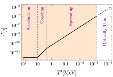
Figure 1: The comoving expansion timescale $\tau^{\prime}$ (solid black line) as a function of the comoving temperature $T^{\prime}$ [cf. Eq. (10)] of a fireball with $T_{0}=100\,\mathinner{\mathrm{MeV}}$, $R_{0}=1\,\text{mm}$, and $\bar{\eta}=10^{-2}$. The three vertical dashed lines mark, from left to right, the transition at $T^{\prime}=T_{0}/\Gamma$ from the acceleration phase to the coasting phase, the transition at $T^{\prime}=T_{0}/\Gamma^{5/3}$ from the coasting phase to the spreading phase, and the point at which photon decoupling occurs [corresponding to $R=R_{\rm thin}$; cf. Eq. (14) with $\varepsilon n_{\bar{p}}\sim n_{\bar{B}}$]. The orange shaded region is thus the region in which the plasma expands as a single tightly coupled fluid through its various expansion phases (as annotated), while the unshaded region where is the region where the plasma has decoupled.

The fluid evolution described above applies as long as the photons remain tightly coupled with the charged particles in the plasma. Eventually, this assumption is violated and the photons decouple; we can estimate when this occurs as follows. Photons in the plasma scatter dominantly with the electrons and positrons, with the Thomson cross section $\sigma_{T}=(8\pi/3)(\alpha^{2}/m_{e}^{2})$. In our parameter space of interest, it is the case that photon decoupling always occurs at a temperature well below the electron mass, after any symmetric thermal population of charged leptons have annihilated away. The opacity of the plasma is then due to the remaining charged leptons that must exist to guarantee net neutrality of the plasma; their identity depends on some details of the BSM injection process because (as we will see) typical expansion timescales are too short for any muon asymmetry that is present to be guaranteed to decay by the time of this decoupling. In what follows, we parametrize the population of residual positrons as having a CoM-frame density $n_{e^{+}}=\varepsilon n_{\bar{p}}$, where $\varepsilon$ can be a BSM-injection dependent parameter, but which we typically expect to be $\varepsilon\sim\mathcal{O}(1)$; because of the $\sigma_{T}\propto m^{-2}$ scaling, residual muons are not relevant to our estimates unless $\varepsilon\lesssim(m_{e}/m_{\mu})^{2}\sim 2\times 10^{-5}$.

The radial optical depth $\kappa(R)$ for a photon emitted from a radius $r\sim R$ inside the shell and escaping to infinity is then [40]

$$\kappa(R) \sim\int_{\sim R}^{\infty}\varepsilon n_{\bar{p}}\sigma_{T}(1-v)dr\sim\kappa_{0}\frac{R_{0}^{2}}{\gamma^{2}R\Delta R}\>,$$ (11)

where the anti-baryon density inside the shell is taken to be roughly constant and scales inversely with the volume of the plasma shell $n_{\bar{B}}\propto 1/(R^{2}\Delta R)$ and $1-v\approx 1/(2\gamma^{2})$ for $v\approx 1$. We have also defined the initial optical depth

$$\kappa_{0} =\varepsilon\bar{\eta}T_{0}^{3}\sigma_{T}R_{0}$$

$$\sim 10^{11}\left(\frac{\bar{\eta}}{10^{-2}}\right)\left(\frac{T_{0}}{100\,\mathinner{\mathrm{MeV}}}\right)^{3}\left(\frac{R_{0}}{1\,\text{mm}}\right)\left(\frac{\varepsilon n_{\bar{p}}}{n_{\bar{B}}}\right)\>,$$ (12)

we have set a leading coefficient $\sim(\zeta(3)/\pi^{2})g_{*}\sim 1$ and neglected other $\mathcal{O}(1)$ factors.

We define $t_{\rm thin}$ to be the rough moment in time where the plasma optical depth for photons in the bulk of the fireball at $r\sim R(t_{\rm thin})$ becomes unity, $\kappa\sim 1$. It turns out that the initial optical depth $\kappa_{0}$ is many orders of magnitude larger than unity in our parameter space of interest; see Eq. (12). This implies that $t_{\rm thin}$ always occurs deep into the final expansion stage (i.e., the spreading stage), and can be estimated as

$$R_{\rm thin} \sim\kappa_{0}^{1/2}R_{0}$$ (13)

$$\sim 300\,\text{m}\times\left(\frac{\bar{\eta}}{10^{-2}}\right)^{1/2}\left(\frac{T_{0}}{100\,\mathinner{\mathrm{MeV}}}\right)^{3/2}$$

$$\qquad\times\left(\frac{R_{0}}{1\,\text{mm}}\right)^{3/2}\left(\frac{\varepsilon n_{\bar{p}}}{n_{\bar{B}}}\right)^{1/2}\>.$$ (14)

At the fiducial parameter point, $\tau^{\prime}(t_{\text{thin}})\sim R_{\text{thin}}/\Gamma\sim 10^{-7}\,\text{s}$, which is less than the rest-frame muon lifetime, as noted above. When the fireball radius hits $R_{\rm thin}$, the bulk of the plasma becomes optically thin and a burst of photons is released. This is also the approximate moment at which the anti-baryons and other particles that were coupled to the fireball plasma (see Sec. III.3) are released into the interstellar medium (see Sec. IV), assuming that the fireball was located in our Galaxy.

III.3 Nuclear physics

The monotonically decreasing co-moving temperature $T^{\prime}(R)$ of the fireball plasma given at Eq. (9) implies that it eventually becomes thermodynamically favorable for bound anti-nuclei to form.

Were thermodynamic equilibrium among the lightest few anti-nuclei species to be achieved (analogous to the situation in Big Bang Nucleosynthesis [BBN]), almost the entirety of the available anti-neutron abundance would be converted into ${}^{4}\overline{\text{He}}$, leading to a final configuration dominated by $\bar{p}$ and ${}^{4}\overline{\text{He}}$, with only trace amounts of other complex light anti-nuclei. Given that AMS-02 has tentatively identified similar numbers of ${}^{3}\overline{\text{He}}$ and ${}^{4}\overline{\text{He}}$ candidates (up to a factor of a few; statistics are small), such an outcome would not be phenomenologically viable.

To understand how to avoid this outcome, consider a key feature of how the analogous process of ordinary BBN proceeds. The most efficient nuclear-reaction pathway to ${}^{4}\text{He}$ has as an initial step free-neutron capture on hydrogen to form deuterium D: $n+p\rightarrow\text{D}+\gamma$ [41], with the D then being processed by further nuclear burning to other light elements. However, the relatively low deuterium binding energy $B_{\text{D}}\approx 2\,\mathinner{\mathrm{MeV}}$ and the low baryon-to-entropy ratio $\eta\approx 6\times 10^{-10}$ during BBN make deuterium prone to photodissociation back to free neutrons and protons: this is the famous “deuterium bottleneck” [42, 43, 44, 45]. Consequently, ${}^{4}\text{He}$ production in BBN was delayed until the temperature of the primordial plasma cooled down significantly below $B_{\text{D}}$, whereupon the abundance of photons capable of dissociating deuterium was considerably Boltzmann suppressed, enabling the deuterium abundance to rise. Crucially, in the BBN realized in our Universe, the deuterium bottleneck was overcome while thermodynamic equilibrium was still being maintained among the light species: nuclear reaction rates were still sufficiently fast compared to Hubble expansion that, once deuterium was capable of being created without being photodissociated, it was rapidly burned to tritium and ${}^{3}\text{He}$, and then further to ${}^{4}\text{He}$.

But standard BBN successfully overcame the deuterium bottleneck while maintaining thermodynamic equilibrium only marginally. If the expansion rate of the Universe were to have been sufficiently larger, neutron capture on hydrogen would have decoupled (i.e., frozen out) before the bottleneck could have been overcome. In that case, the output of the nucleosynthesis would not have been dictated by thermodynamic equilibrium among the light nuclei. Instead, the immediate nucleosynthesis products in this scenario would have been mostly free protons and neutrons, with smaller abundances of deuterium, tritium, ${}^{3}\text{He}$, and ${}^{4}\text{He}$ being produced in amounts controlled by the relative rates of nuclear reactions that produce them, which can be comparable to one another. Accounting for the fact that unstable neutrons later decay to protons and tritium later decays to ${}^{3}\text{He}$, the final output in this counterfactual case could easily have been such that $n_{p}\gg n_{{}^{3}\text{He}}\sim n_{{}^{4}\text{He}}$.

In what follows, we show that parameter space exists for which the analogous anti-nucleosynthesis occurring in our expanding fireball remains in this “stuck in the bottleneck” regime, yielding phenomenologically viable amounts of ${}^{3}\overline{\text{He}}$ as compared to ${}^{4}\overline{\text{He}}$.

III.3.1 Preliminaries

In order to separate changes in the number density of an element due to nuclear reactions from that due to the fireball expansion, in this section we describe the evolution of a nuclear species $i$ in terms of its fractional abundance $X_{i}$, defined as

$$X_{i}\equiv\frac{n_{i}^{\prime}}{n_{\bar{B}}^{\prime}}\>,$$ (15)

where $n_{i}^{\prime}$ is the number density of element $i$ and $n^{\prime}_{\bar{B}}$ is the anti-baryon number density. We consider only $i\in\{\bar{p},\bar{n},{\mkern-2.0mu\bar{\mkern 2.0mu\text{D}}},{\bar{\text{T}}},{}^{3}\overline{\text{He}},{}^{4}\overline{\text{He}}\}$. We obtain the evolution of the abundances of nuclear elements $X_{i}$ by numerically solving the Boltzmann equations detailed in Appendix C describing the simplified network of nuclear reactions among these species, using the nuclear cross sections shown in Appendix D. The results of these numerical computations are summarized in Figs. 2–5.

While those numerical results are of course more accurate, we also wish to gain an understanding of, and intuition for, the most important nuclear processes at work, and determine the dependencies of the final anti-helium isotope abundances on the fireball parameters $(T_{0},R_{0},\bar{\eta})$. In what follows, we therefore develop an analytical understanding that reproduces the gross features of the numerical results.

The main approximation we employ in our analytical arguments is as follows. In general, nuclear species with higher mass numbers $A$ are produced from those with lower $A$ in a sequence of successive two-body nuclear reactions. Our numerical analysis shows that in the fireball parameter space that yields $X_{{}^{3}\overline{\text{He}}}\gtrsim X_{{}^{4}\overline{\text{He}}}$, a hierarchy is maintained between the nuclear abundances with successive mass numbers, namely $X_{\bar{n}}+X_{\bar{p}}\gtrsim X_{{\mkern-2.0mu\bar{\mkern 2.0mu\text{D}}}}\gtrsim X_{{\bar{\text{T}}}}+X_{{}^{3}\overline{\text{He}}}\gtrsim X_{{}^{4}\overline{\text{He}}}$, as depicted in Figs. 2 and 3. Furthermore, that analysis shows that anti-nucleosynthesis occurs mainly at temperatures $T^{\prime}\sim 100-200\,\mathinner{\mathrm{keV}}$ low enough that all of the endothermic reverse nuclear reactions to the exothermic ones considered in this subsection are negligible, except for the photodissociation of anti-deuterium responsible for the bottleneck in the first place, which we thus take into account in our analysis. These observations suggest that, instead of solving the whole nuclear reaction network at once, we can treat the nuclear reactions sequentially; that is, we can consider elements produced earlier in the chain of successive two-body reactions as fixed sources for reactions later in the chain of successive reactions, neglecting back-reaction on those sources arising from those later reactions.

In what follows, we first discuss relevant expansion timescales, and then proceed to discuss in turn heavier and heavier anti-nuclei synthesized in this approximate sequential paradigm. Finally, we summarize and discuss other, non–anti-nucleosynthetic outputs.

III.3.2 Expansion timescales

Anti-nucleosynthesis in the fluid rest frame of the expanding fireball is qualitatively similar to BBN in that there are various nuclear reactions occurring in an adiabatically expanding background [42, 43, 44, 45]. However, it differs from the BBN in important ways. The plasma in our scenario is spatially finite and expands relativistically into vacuum. This of course leads to a non-trivial dependence of the dynamical expansion timescale $\tau^{\prime}$ on the comoving temperature $T^{\prime}$, as shown at Eq. (10).

The parameter space that is viable for our model is roughly $10^{-4}\,\text{m}\lesssim R_{0}\lesssim 1\,\text{m}$ (i.e., $10^{-13}\,\text{s}\lesssim\tau_{0}\lesssim 10^{-9}\,\text{s}$), $10\,\mathinner{\mathrm{MeV}}\lesssim T_{0}\lesssim 200\,\mathinner{\mathrm{MeV}}$, and $\Gamma\sim T_{0}/\bar{\eta}m_{p}\sim 10$ (i.e., $10^{-3}\lesssim\bar{\eta}\lesssim 10^{-2}$). We displayed the scalings of $\tau^{\prime}(T^{\prime})$ in Fig. 1 for benchmark parameters in these ranges. The results are quantitatively and qualitatively very different compared to the Hubble time as a function of temperature during BBN; as we will see, this leads to important differences between fireball anti-nucleosynthesis and BBN. As we will show, fireball anti-nucleosynthesis in this parameter space commences at temperature $100\,\mathinner{\mathrm{keV}}\lesssim T_{{\mkern-2.0mu\bar{\mkern 2.0mu\text{D}}}}^{\prime}\lesssim 200\,\mathinner{\mathrm{keV}}$, which satisfies $T_{{\mkern-2.0mu\bar{\mkern 2.0mu\text{D}}}}^{\prime}\lesssim T_{0}/\Gamma^{5/3}$ and thereby always falls in the “spreading” phase of the fireball expansion.

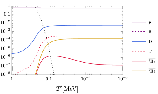
Figure 2: The abundances of nuclear species $X_{i}=n^{\prime}_{i}/n^{\prime}_{\bar{B}}$ (solid and dashed colored lines, as identified in the legend) as a function of the comoving fireball temperature $T^{\prime}$, computed by numerically solving the Boltzmann equations for a simplified nuclear-reaction network detailed in Appendix C, for a fireball with $T_{0}=100\,\mathinner{\mathrm{MeV}}$, $R_{0}=1.5\,\text{mm}$, $\bar{\eta}=10^{-2}$ ($\Gamma=10$). Also shown is $Y_{{\mkern-2.0mu\bar{\mkern 2.0mu\text{D}}},\gamma}=n^{\prime}_{\gamma}(E^{\prime}_{\gamma}>Q_{D})/n^{\prime}_{\bar{B}}$ (dotted black line), the abundance of photons with energies $E^{\prime}_{\gamma}$ above the anti-deuteron photodissociation threshold $Q_{D}$. Initially, nuclear bound states are essentially non-existent, apart from ${\mkern-2.0mu\bar{\mkern 2.0mu\text{D}}}$ whose abundance is kept at an exponentially small value due to the high abundance of photodissociating photons, $Y_{{\mkern-2.0mu\bar{\mkern 2.0mu\text{D}}},\gamma}\gg X_{{\mkern-2.0mu\bar{\mkern 2.0mu\text{D}}}}$. As the fireball cools down, $Y_{{\mkern-2.0mu\bar{\mkern 2.0mu\text{D}}},\gamma}$ decreases while $X_{{\mkern-2.0mu\bar{\mkern 2.0mu\text{D}}}}$ increases. Eventually at $T=T^{\prime}_{{\mkern-2.0mu\bar{\mkern 2.0mu\text{D}}}}\sim 140\,\mathinner{\mathrm{keV}}$ [cf. Eq. (26)], $Y_{{\mkern-2.0mu\bar{\mkern 2.0mu\text{D}}},\gamma}$ drops sufficiently low that photodissociation becomes inefficient, thus marking the onset of anti-nucleosynthesis: the absence of photodissociation allows $X_{{\mkern-2.0mu\bar{\mkern 2.0mu\text{D}}}}$ to rise significantly, which enables nuclear reactions involving ${\mkern-2.0mu\bar{\mkern 2.0mu\text{D}}}$ to produce ${\bar{\text{T}}}$ whose presence, in turn, enables the production of ${}^{4}\overline{\text{He}}$. The rise in $X_{{\mkern-2.0mu\bar{\mkern 2.0mu\text{D}}}}$ also enables ${}^{3}\overline{\text{He}}$ production but the produced ${}^{3}\overline{\text{He}}$ quickly converts into ${\bar{\text{T}}}$. Since the nuclear reaction rates are proportional to the antibaryon number density $n^{\prime}_{\bar{B}}\propto T^{\prime 3}$, most of the anti-nucleus production occurs within the first few $e$-foldings of expansion after $Y_{{\mkern-2.0mu\bar{\mkern 2.0mu\text{D}}},\gamma}$ drops below $X_{{\mkern-2.0mu\bar{\mkern 2.0mu\text{D}}}}$. Nuclear species depicted in dashed lines are stable in the timescale of fireball evolution (until it becomes optically thin) but are expected to decay to the species shown by the solid line of the same color during their journey to the solar system.

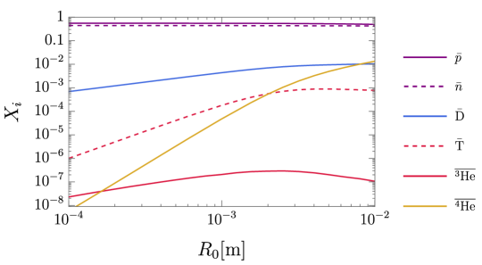
Figure 3: The abundances of nuclear species $X_{i}=n^{\prime}_{i}/n^{\prime}_{\bar{B}}$ (with $i$ as annotated in the legend) released when a fireball with an initial radius $R_{0}$ becomes optically thin, computed by numerically solving the Boltzmann equations for a simplified nuclear-reaction network, as detailed in Appendix C. Here, we set $T_{0}=100\,\mathinner{\mathrm{MeV}}$ and $\bar{\eta}=10^{-2}$ ($\Gamma=10$). While the hierarchy $X_{\bar{p}}\approx X_{\bar{n}}\gtrsim X_{{\mkern-2.0mu\bar{\mkern 2.0mu\text{D}}}}\gtrsim X_{{\bar{\text{T}}}}\gtrsim X_{{}^{4}\overline{\text{He}}}$ is maintained, the abundances of ${\mkern-2.0mu\bar{\mkern 2.0mu\text{D}}}$, ${\bar{\text{T}}}$, ${}^{4}\overline{\text{He}}$ released by the fireball scale with $R_{0}$, respectively, as $X_{{\mkern-2.0mu\bar{\mkern 2.0mu\text{D}}}}\propto R_{0}$ [cf. Eq. (29)], $X_{{\bar{\text{T}}}}\propto X_{{\mkern-2.0mu\bar{\mkern 2.0mu\text{D}}}}^{2}\propto R_{0}^{2}$ [cf. Eq. (31)], $X_{{}^{4}\overline{\text{He}}}\propto X_{{\bar{\text{T}}}}X_{{\mkern-2.0mu\bar{\mkern 2.0mu\text{D}}}}^{2}\propto R_{0}^{4}$ [cf. Eq. (33)]. Besides that, ${}^{3}\overline{\text{He}}$ is produced promptly in negligible amount, $X_{{}^{3}\overline{\text{He}}}\lesssim 10^{-6}$ [cf. Eq. (32)]. Nuclear species depicted in dashed lines are stable on the timescale of the fireball evolution (until it becomes optically thin) but are expected to subsequently decay to the species shown in with solid lines of the same color on timescales short compared to their propagation time in the Milky Way (e.g., ${\bar{\text{T}}}$ later decays to ${}^{3}\overline{\text{He}}$ with a half-life of $\sim 12$ years in the ${\bar{\text{T}}}$ rest frame).

III.3.3 Anti-nucleon abundance

At temperatures $10\,\mathinner{\mathrm{MeV}}\lesssim T^{\prime}\lesssim 200\,\mathinner{\mathrm{MeV}}$, nuclear bound states have not formed and all the anti-baryons reside in unbound anti-neutrons and anti-protons. Anti-neutrons can, in principle, convert to and from anti-protons through both weak (e.g., $\bar{n}+e^{-}\leftrightarrow\bar{p}+\nu_{e}$) and strong (e.g., $\bar{n}+\pi^{-}\leftrightarrow\bar{p}+\pi^{0}$) processes [54, 31, 32]. If at least one of these processes is efficient, the relative abundance of these anti-nucleons is initially kept at its chemical equilibrium value, $n^{\prime}_{\bar{n}}/n^{\prime}_{\bar{p}}=\text{exp}\left[-(m_{n}-m_{p})/T^{\prime}\right]$. In the early Universe, the matter analogue of both processes were efficient at some point after hadronization. Then, strong processes decouple first as pions rapidly decay and annihilate away, and hence the pre-BBN freeze-out abundances of neutrons and protons were determined by the later-occurring decoupling of weak interactions. By contrast, in the fireball anti-nucleosynthesis scenario we consider, the typically short timescales of the fireball expansion render weak interactions inefficient at all times. Consequently, the anti-nucleons freeze out as soon as the pion-mediated strong interconversion processes become inefficient.

After the fireball has thermalized, the following strong-mediated charge exchange reactions (SMCER) are initially in equilibrium [30] (see discussion about $T^{\prime}_{\bar{n}\bar{p}}$ below)

$$\bar{p}+\pi^{+}\leftrightarrow\bar{n}+\pi^{0}\quad(Q=5.9\mathinner{\mathrm{MeV}})\>;$$

$$\bar{n}+\pi^{-}\leftrightarrow\bar{p}+\pi^{0}\quad(Q=3.3\mathinner{\mathrm{MeV}})\>.$$

Additionally, $\mu_{\gamma}=0$, $\mu_{\pi^{0}}=0$, and $\mu_{\pi^{-}}=-\mu_{\pi^{+}}$. These imply

$$\mu_{\bar{n}}-\mu_{\bar{p}}=\mu_{\pi^{+}}\>.$$ (16)

The chemical equilibrium anti-neutron–to–anti-proton ratio for $T^{\prime}\ll m_{n}-\mu_{\bar{n}},m_{p}-\mu_{\bar{p}}$ is thus given by

$$\left(\frac{n_{\bar{n}}^{\prime}}{n_{\bar{p}}^{\prime}}\right)_{\rm ch}\approx e^{-\frac{m_{n}-m_{p}}{T^{\prime}}+\frac{\mu_{\pi^{+}}}{T^{\prime}}}\>.$$ (17)

where $m_{n}-m_{p}\approx 1.3\mathinner{\mathrm{MeV}}$. Note that the chemical potential of the charged pions, $\mu_{\pi^{+}}$, depends on the physics before the fireball has thermalized via efficient strong and EM interactions. Therefore, it is model-dependent. For instance, it depends on whether electroweak interactions were ever efficient in this pre-thermalization stage, and on some details of the BSM particle injection process that seeds the fireball. For simplicity, we neglect the chemical potential of charged pion in our analysis here by assuming

$$\left|\mu_{\pi^{+}}\right|\ll m_{n}-m_{p}\>.$$ (18)

We discuss the model-dependence of $\mu_{\pi^{+}}$ and the case when $\mu_{\pi^{+}}$ is non-negligible in Appendix B.

The pion-mediated strong interactions decouple at a temperature $T^{\prime}=T^{\prime}_{\bar{n}\bar{p}}$ where the pion abundance becomes sufficiently Boltzmann suppressed that the $\Gamma_{\rm strong}(T^{\prime})$ found in Eq. (1) goes below the fireball expansion rate $1/\tau^{\prime}$ found in Eq. (10). We find that, numerically, $T^{\prime}_{\bar{n}\bar{p}}\approx 6\,\mathinner{\mathrm{MeV}}$ invariably in the whole parameter space that is viable for our scenario. The freeze-out value of the anti-neutron–to–anti-proton ratio $n^{\prime}_{\bar{n}}/n^{\prime}_{\bar{p}}$ can be approximated by its chemical-equilibrium value at that time

$$\left.\frac{n^{\prime}_{\bar{n}}}{n^{\prime}_{\bar{p}}}\right|_{{\rm ch},\,T_{\bar{n}\bar{p}}^{\prime}}\approx e^{-(m_{n}-m_{p})/T_{\bar{n}\bar{p}}^{\prime}}\approx 0.8\>.$$ (19)

If $\left|\mu_{\pi^{+}}\right|\gtrsim m_{n}-m_{p}$, unlike what we have assumed, then the freeze-out value of $n^{\prime}_{\bar{n}}/n^{\prime}_{\bar{p}}$ and our subsequent results would change; however, as long as $\left|\mu_{\pi^{+}}\right|\lesssim T^{\prime}_{\bar{n}\bar{p}}\approx 6\mathinner{\mathrm{MeV}}$, these changes are only $\mathcal{O}(1)$ and most of our conclusions remain valid. See Appendix B for further discussion.

Moreover, while neutron decay is an important phenomenon in the BBN that was realized in the early Universe, in our scenario anti-neutrons do not decay until well after anti-nucleosynthesis finishes. Assuming that only a small fraction of the $\bar{p}$ and $\bar{n}$ are burned to higher nuclei (true throughout our parameter space of interest), we will thus have, for all times relevant for the anti-nucleosynthesis in the expanding fireball, the following:

$$X_{\bar{n}}(T^{\prime}) \approx X_{\bar{n}}(T^{\prime}_{\bar{n}\bar{p}})\equiv X^{\text{ch}}_{\bar{n}};$$ (20)

$$X_{\bar{p}}(T^{\prime}) \approx X_{\bar{p}}(T^{\prime}_{\bar{n}\bar{p}})\equiv X^{\text{ch}}_{\bar{p}}\>,$$ (21)

where

$$X^{\text{ch}}_{\bar{n}} \approx 0.8X^{\text{ch}}_{\bar{p}}\>, X^{\text{ch}}_{\bar{n}}+X^{\text{ch}}_{\bar{p}} \approx 1\>,$$ (22)

implying that

$$X^{\text{ch}}_{\bar{n}} \approx 0.44\>, X^{\text{ch}}_{\bar{p}} \approx 0.56\>.$$ (23)

III.3.4 Anti-deuterium production

Anti-deuterium is produced primarily through the reaction $\bar{n}+\bar{p}\rightarrow{\mkern-2.0mu\bar{\mkern 2.0mu\text{D}}}+\gamma$. Initially, however, the reverse reaction (photodissociation) is in equilibrium and the high abundance of photons with energies above the anti-deuterium binding energy $B_{{\mkern-2.0mu\bar{\mkern 2.0mu\text{D}}}}\approx 2.2\,\mathinner{\mathrm{MeV}}$ suppresses the (quasi-equilibrium) anti-deuterium abundance, which is given by the Saha equation:

$$X_{{\mkern-2.0mu\bar{\mkern 2.0mu\text{D}}},\rm ch}\approx\bar{\eta}\left(\frac{T^{\prime}}{m_{p}}\right)^{3/2}e^{B_{\mkern-2.0mu\bar{\mkern 2.0mu\text{D}}}/T^{\prime}}.$$ (24)

This continues until the abundance of photons with sufficient energy to photodissociate anti-deuterium,

$$Y_{{\mkern-2.0mu\bar{\mkern 2.0mu\text{D}}}\gamma}=\frac{n^{\prime}_{\gamma}(E^{\prime}_{\gamma}\gtrsim B_{\mkern-2.0mu\bar{\mkern 2.0mu\text{D}}})}{n^{\prime}_{\bar{B}}}\sim\frac{1}{\bar{\eta}}\frac{B_{\mkern-2.0mu\bar{\mkern 2.0mu\text{D}}}^{2}}{T^{\prime 2}}e^{-B_{\mkern-2.0mu\bar{\mkern 2.0mu\text{D}}}/T^{\prime}}\>,$$ (25)

starts to fall below the anti-deuterium abundance; i.e., $Y_{{\mkern-2.0mu\bar{\mkern 2.0mu\text{D}}}\gamma}\sim X_{{\mkern-2.0mu\bar{\mkern 2.0mu\text{D}}}}$. The temperature at that point can be estimated as

$$T_{{\mkern-2.0mu\bar{\mkern 2.0mu\text{D}}}}^{\prime} \approx\frac{B_{\mkern-2.0mu\bar{\mkern 2.0mu\text{D}}}}{4.6-\ln\bar{\eta}+(7/4)\ln\left(4.6-\ln\bar{\eta}\right)}$$

$$\approx 140-170\,\mathinner{\mathrm{keV}},$$ (26)

where the displayed range of values $T_{{\mkern-2.0mu\bar{\mkern 2.0mu\text{D}}}}^{\prime}$ corresponds to the range of viable anti-baryon–to–entropy ratios $10^{-3}\lesssim\bar{\eta}\lesssim 10^{-2}$. As mentioned earlier, in our the parameter space of interest $T_{\mkern-2.0mu\bar{\mkern 2.0mu\text{D}}}^{\prime}$ falls in the spreading phase of the fireball expansion (i.e., it satisfies $T_{\mkern-2.0mu\bar{\mkern 2.0mu\text{D}}}^{\prime}\lesssim T_{0}/\Gamma^{5/3}$) and, neglecting the mild logarithmic dependence on $\bar{\eta}$, the fireball expansion timescale at decoupling of the photodissociation reactions is

$$\tau^{\prime}_{{\mkern-2.0mu\bar{\mkern 2.0mu\text{D}}}} \equiv\tau^{\prime}(T_{{\mkern-2.0mu\bar{\mkern 2.0mu\text{D}}}}^{\prime})$$

$$\approx 5.1\times 10^{-10}\,\text{s}\left(\frac{T_{0}}{100\,\mathinner{\mathrm{MeV}}}\right)\left(\frac{R_{0}}{\text{mm}}\right)\left(\frac{\Gamma}{10}\right)^{-2/3}\>,$$ (27)

where we have set $T_{{\mkern-2.0mu\bar{\mkern 2.0mu\text{D}}}}^{\prime}=140\mathinner{\mathrm{keV}}$ (corresponding to $\bar{\eta}=10^{-3}$). After the photodissociation of ${\mkern-2.0mu\bar{\mkern 2.0mu\text{D}}}$ decouples at $T_{\mkern-2.0mu\bar{\mkern 2.0mu\text{D}}}^{\prime}$, at which point the fireball expansion timescale is $\tau^{\prime}_{{\mkern-2.0mu\bar{\mkern 2.0mu\text{D}}}}$, anti-deuterium production through $\bar{n}+\bar{p}\rightarrow{\mkern-2.0mu\bar{\mkern 2.0mu\text{D}}}+\gamma$ is no longer thwarted, and so the anti-deuterium abundance rises monotonically. At around the same time, heavier elements that rely on anti-deuterium burning as an initial step begin to be populated sequentially. Since the product of the fireball expansion timescale and the nuclear reaction rates that form any of the light elements scales as $\propto n^{\prime}_{\bar{B}}\left<\sigma v\right>\tau^{\prime}\propto T^{\prime 2}$ during the spreading phase ($T^{\prime}\lesssim T_{0}/\Gamma^{5/3}$), these nuclear reactions are most efficient in populating the light elements in the first fireball-expansion $e$-fold or so after the decoupling of ${\mkern-2.0mu\bar{\mkern 2.0mu\text{D}}}$ photodissociation (when anti-baryon density is the highest), before the anti-baryon density is significantly diluted by the expansion.

Moreover, as we operate in the regime where anti-deuterium is not efficiently burned to more complex nuclei (see the next sub-subsection), a simple estimate for the final anti-deuterium abundance can be obtained by assuming the anti-deuterium abundance is that generated by neutron–proton fusion reactions operating in a single dynamical expansion timescale at the point of anti-deuterium photodissociation freeze-out. We estimate that abundance to be

$$X^{\text{prompt}}_{{\mkern-2.0mu\bar{\mkern 2.0mu\text{D}}}} \approx k_{\bar{2}}n^{\prime}_{\bar{B}}\left<\sigma v\right>_{\bar{n}\bar{p}}\tau^{\prime}_{{\mkern-2.0mu\bar{\mkern 2.0mu\text{D}}}}X_{\bar{n}}^{\text{ch}}X_{\bar{p}}^{\text{ch}}$$ (28)

$$\approx 4.0\times 10^{-3}\times\left(\frac{k_{\bar{2}}}{0.60}\right)$$

$$\qquad\times\left(\frac{T_{0}}{100\,\mathinner{\mathrm{MeV}}}\right)^{2}\left(\frac{R_{0}}{\text{mm}}\right)\left(\frac{\Gamma}{10}\right)^{-5/3},$$ (29)

where we took the value of cross-section $\left<\sigma v\right>_{\bar{n}\bar{p}}$ to be that at $T^{\prime}\sim 140\,\mathinner{\mathrm{keV}}$ (the lower end of the range of values for $T^{\prime}_{{\mkern-2.0mu\bar{\mkern 2.0mu\text{D}}}}$); see Appendix D. In writing the above results, we have used $\bar{\eta}\sim T_{0}/(\Gamma m_{p})$ and we manually inserted an $\mathcal{O}(1)$ prefactor $k_{\bar{2}}\approx 0.60$ in Eq. (28), such that the final result is in better agreement with what we obtained by numerically solving the Boltzmann equations at this benchmark point.

We are interested in the regime where $X^{\text{prompt}}_{{\mkern-2.0mu\bar{\mkern 2.0mu\text{D}}}}\ll 1$: i.e., the anti-deuterium production decouples before its abundance rises to $X_{{\mkern-2.0mu\bar{\mkern 2.0mu\text{D}}}}\sim 1$.

III.3.5 Anti-deuterium burning

During and slightly after the production of anti-deuterium, a small fraction of it also burns through the following dominant channels:

$${\mkern-2.0mu\bar{\mkern 2.0mu\text{D}}}+{\mkern-2.0mu\bar{\mkern 2.0mu\text{D}}} \rightarrow{}^{3}\overline{\text{He}}+\bar{n}\>,$$

$${\mkern-2.0mu\bar{\mkern 2.0mu\text{D}}}+{\mkern-2.0mu\bar{\mkern 2.0mu\text{D}}} \rightarrow{\bar{\text{T}}}+\bar{p}\>,$$

with essentially equal branching fractions (both are strong-mediated nuclear reactions). Because we are analyzing production in the regime where anti-deuterium is not efficiently burned to more complex anti-nuclei, we may treat the abundance of anti-deuterium as a fixed source which acts to populate the more complex nuclei over roughly a single dynamical expansion timescale after the anti-deuterium are produced. As such, the prompt production of ${}^{3}\overline{\text{He}}$ and ${\bar{\text{T}}}$ can be estimated as

$$X_{{\bar{\text{T}}}}^{\text{prompt}}\approx X_{{}^{3}\overline{\text{He}}}^{\text{prompt}}\approx k_{\bar{3}}n^{\prime}_{\bar{B}}\left<\sigma v\right>_{{\mkern-2.0mu\bar{\mkern 2.0mu\text{D}}}{\mkern-2.0mu\bar{\mkern 2.0mu\text{D}}}}\tau^{\prime}_{{\mkern-2.0mu\bar{\mkern 2.0mu\text{D}}}}(X^{\text{prompt}}_{{\mkern-2.0mu\bar{\mkern 2.0mu\text{D}}}})^{2}\>,$$ (30)

where we have evaluated all the quantities at $T^{\prime}\sim T^{\prime}_{{\mkern-2.0mu\bar{\mkern 2.0mu\text{D}}}}$, assumed $X_{{\mkern-2.0mu\bar{\mkern 2.0mu\text{D}}}}\gg X_{{}^{3}\overline{\text{He}}},X_{{\bar{\text{T}}}}$ around the time of this production, and manually included an $\mathcal{O}(1)$ numerical prefactor $k_{\bar{3}}\approx 0.15$ [cf. the factor $k_{\bar{2}}$ introduced in Eq. (28)].

Alternative production channels for ${}^{3}\overline{\text{He}}$ and ${\bar{\text{T}}}$ are ${\mkern-2.0mu\bar{\mkern 2.0mu\text{D}}}+\bar{p}\rightarrow{}^{3}\overline{\text{He}}+\gamma$ and ${\mkern-2.0mu\bar{\mkern 2.0mu\text{D}}}+\bar{n}\rightarrow{\bar{\text{T}}}+\gamma$, respectively; however, we verified numerically that the former production channel is negligible as long as $X_{{\mkern-2.0mu\bar{\mkern 2.0mu\text{D}}}}\gg 10^{-5}$ and the latter is negligible as long as $X_{{\mkern-2.0mu\bar{\mkern 2.0mu\text{D}}}}\gg 10^{-4}$, which are always satisfied in the parameter space we consider. It is understood that these process are inefficient because they both suffer from photon-emission suppression (i.e., they are electromagnetic-mediated, rather than strong-mediated, nuclear reactions).

The reaction ${\mkern-2.0mu\bar{\mkern 2.0mu\text{D}}}+{\mkern-2.0mu\bar{\mkern 2.0mu\text{D}}}\rightarrow{}^{4}\overline{\text{He}}+\gamma$ can also proceed with a branching ratio of $\sim 10^{-7}$ (it is electromagnetically mediated). Because of this small branching fraction, prompt ${}^{4}\overline{\text{He}}$ production through this channel, $X^{\text{prompt}}_{{}^{4}\overline{\text{He}}}\sim n^{\prime}_{\bar{B}}(10^{-7}\left<\sigma v\right>_{{\mkern-2.0mu\bar{\mkern 2.0mu\text{D}}}{\mkern-2.0mu\bar{\mkern 2.0mu\text{D}}}})\tau_{{\mkern-2.0mu\bar{\mkern 2.0mu\text{D}}}}^{\prime}(X^{\text{prompt}}_{{\mkern-2.0mu\bar{\mkern 2.0mu\text{D}}}})^{2}$, is negligible compared to other, deuterium–tritium-burning channels that we discuss below so long as $X_{{\bar{\text{T}}}}/X_{{\mkern-2.0mu\bar{\mkern 2.0mu\text{D}}}}\gg 10^{-7}$ around the time of production.

III.3.6 Anti-helium-3 burning

The strong-mediated reaction ${}^{3}\overline{\text{He}}+\bar{n}\rightarrow{\bar{\text{T}}}+\bar{p}$ is also present. It is also extremely efficient in part because it is not Coulomb suppressed. It thus gives the one counterexample to our earlier statement that we can ignore back-reaction on sequentially produced species: this reaction burns essentially all the anti-helium-3 that are produced primarily (via ${\mkern-2.0mu\bar{\mkern 2.0mu\text{D}}}+{\mkern-2.0mu\bar{\mkern 2.0mu\text{D}}}\rightarrow{}^{3}\overline{\text{He}}+\bar{n}$) to anti-tritium. As such, the anti-helium-3 abundance is maintained at a very low, quasi-equilibrium level: we numerically found that the residual $X_{{}^{3}\overline{\text{He}}}$ never exceeds $\sim 10^{-6}$. At the same time, the ${\bar{\text{T}}}$ abundance is roughly doubled because our estimate at Eq. (30) indicated roughly equal production abundances for the two $A=3$ anti-nuclei before this depletion reaction was accounted for. Our estimates of the anti-tritium and anti-helium-3 abundances after this burning should therefore be revised to

$$X^{\text{burn}}_{{\bar{\text{T}}}} \approx 2X^{\text{prompt}}_{{\bar{\text{T}}}}\approx 2k_{\bar{3}}n^{\prime}_{\bar{B}}\left<\sigma v\right>_{{\mkern-2.0mu\bar{\mkern 2.0mu\text{D}}}{\mkern-2.0mu\bar{\mkern 2.0mu\text{D}}}}\tau^{\prime}_{{\mkern-2.0mu\bar{\mkern 2.0mu\text{D}}}}(X^{\text{prompt}}_{{\mkern-2.0mu\bar{\mkern 2.0mu\text{D}}}})^{2}\>,$$ (31)

$$X^{\text{burn}}_{{}^{3}\overline{\text{He}}} \lesssim 10^{-6}\>.$$ (32)

III.3.7 Anti-tritium burning

Anti-tritium burns efficiently to anti-helium-4 through the following dominant process:

$${\bar{\text{T}}}+{\mkern-2.0mu\bar{\mkern 2.0mu\text{D}}} \rightarrow{}^{4}\overline{\text{He}}+\bar{n}\>;$$

assuming that $X_{{\bar{\text{T}}}}\gtrsim X_{{}^{4}\overline{\text{He}}}$ throughout the burning, we find that the prompt production is

$$X^{\text{prompt}}_{{}^{4}\overline{\text{He}}}\approx k_{\bar{4}}n^{\prime}_{\bar{B}}\left<\sigma v\right>_{{\bar{\text{T}}}{\mkern-2.0mu\bar{\mkern 2.0mu\text{D}}}}\tau_{{\mkern-2.0mu\bar{\mkern 2.0mu\text{D}}}}^{\prime}X_{{\bar{\text{T}}}}^{\text{burn}}X_{{\mkern-2.0mu\bar{\mkern 2.0mu\text{D}}}}^{\text{prompt}}\>,$$ (33)

where we again manually introduced an $\mathcal{O}(1)$ prefactor $k_{\bar{4}}\approx 0.20$ to better match our numerical results.

III.3.8 Final anti-nucleosynthesis products

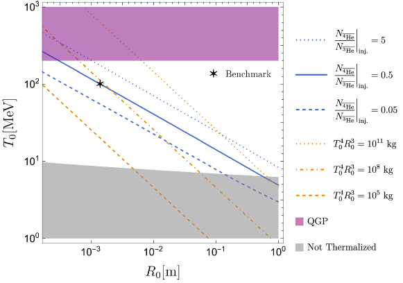
Figure 4: The fireball parameter space. The initial temperature $T_{0}$ and radius $R_{0}$ of the fireball are defined at the point right after the fireball plasma has reorganized itself into a shell moving with an average Lorentz factor $\gamma\sim\text{few}$. The various styles of blue lines show contours of constant values of ratio of the injected anti-helium-4 and anti-helium-3 abundances, $N_{{}^{4}\overline{\text{He}}}/N_{{}^{3}\overline{\text{He}}}|_{\text{inj.}}$. These contours were obtained by numerically solving the Boltzmann equations for a simplified nuclear-reaction network detailed in Appendix C, while fixing the anti-baryon–to–entropy ratio $\bar{\eta}$ such that the terminal Lorentz factor of the shell is $\Gamma\sim T_{0}/(\bar{\eta}m_{p})=10$. The orange lines show contours of constant $T_{0}^{4}R_{0}^{3}$, and provide estimates, up to numerical factors, of the total injection energy in the form of anti-quarks required to create the fireball corresponding to a parameter space point of interest. The black star indicates the benchmark parameter point defined at Eq. (43). The purple region is the parameter space where the fireball would thermalize at a temperature above the QCD phase transition (making it a quark–gluon plasma [QGP]), a regime we avoid to keep our analysis tractable. In the the gray region, the would-be temperature of the fireball $T_{0}$ is so low that pions are too Boltzmann suppressed to facilitate the thermalization of the injected anti-quarks; i.e., $\Gamma_{\rm strong}(T_{0})\lesssim R_{0}^{-1}$.

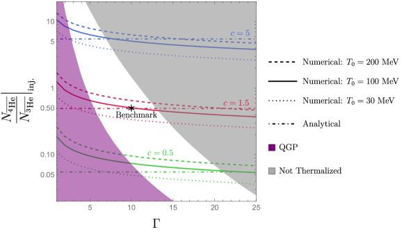
Figure 5: Output space. The injected anti-helium isotope ratio $N_{{}^{4}\overline{\text{He}}}/N_{{}^{3}\overline{\text{He}}}|_{\text{inj.}}$ and the typical injected Lorentz factors $\Gamma$ of the anti-particles are two key observables we seek to explain with the fireball anti-nucleosynthesis scenario we propose in this paper. Publicly available AMS-02 tentative data currently favor observed values of $N_{{}^{4}\overline{\text{He}}}/N_{{}^{3}\overline{\text{He}}}|_{\text{obs.}}\approx 1/2$ and $\Gamma\sim 10$ (this figure does not include propagation effects; see Sec. IV). Dashed and dotted lines show the injected anti-helium isotope ratio $N_{{}^{4}\overline{\text{He}}}/N_{{}^{3}\overline{\text{He}}}|_{\text{inj.}}$ obtained by numerically solving the Boltzmann equations for a simplified nuclear-reaction network detailed in Appendix C, while dot-dashed lines show the analytical approximation, Eq. (41). The black star indicates the benchmark parameter point defined at Eq. (43). The analytical prediction on the anti-helium isotope ratio has a precise quadratic dependence $N_{{}^{4}\overline{\text{He}}}/N_{{}^{3}\overline{\text{He}}}|_{\text{inj.}}\propto c^{2}$ on the combination of parameters $c\equiv(T_{0}/100\,\mathinner{\mathrm{MeV}})^{2}(R_{0}/\text{mm})(\Gamma/10)^{-5/3}$; although it is only strictly speaking valid when $c\lesssim 2.1$ [see discussion below Eq. (42)], we also show it here for $c=5$, where it is still reasonably accurate. The numerical computation of $N_{{}^{4}\overline{\text{He}}}/N_{{}^{3}\overline{\text{He}}}|_{\text{inj.}}$ confirms the expected strong dependence on $c$, but it also shows mild sensitivity to $(T_{0},R_{0},\Gamma)$ variation orthogonal to $c$. Shown in purple is the parameter space where fireball thermalizes into a quark gluon plasma (QGP), a regime we avoid to keep our analysis tractable. In the parameter space colored in gray, the would-be temperature of the fireball $T_{0}$ is so low that pions are too Boltzmann suppressed to facilitate the thermalization of the injected anti-quarks; i.e., $\Gamma_{\rm strong}(T_{0})\lesssim R_{0}^{-1}$.

Anti-neutrons have a mean rest-frame lifetime of $\mathcal{O}(15)$ minutes (decaying to an anti-proton), while anti-tritium decays to anti-helium-3 via the beta decay ${\bar{\text{T}}}\rightarrow{}^{3}\overline{\text{He}}+e^{+}+\nu_{e}$ with a rest-frame half-life of 12.3 years. Even accounting for Lorentz factors $\Gamma\sim 10$, the $\bar{n}$ and ${\bar{\text{T}}}$ will decay on $\mathcal{O}(100)\,\text{yr}$ timescales (at most) as viewed in the fireball center-of-mass frame. After these decays, the remaining light anti-nuclei outputs of our scenario are, at late time, given by

$$X_{\bar{p}} \approx 1\>,$$ (34)

$$X_{{\mkern-2.0mu\bar{\mkern 2.0mu\text{D}}}} \approx X^{\text{prompt}}_{{\mkern-2.0mu\bar{\mkern 2.0mu\text{D}}}}\qquad\text{[see Eq{}.~{}(\ref{eq:XD})]}\>,$$ (35)

$$X_{{}^{3}\overline{\text{He}}} \approx X_{{\bar{\text{T}}}}^{\text{burn}}$$

$$\approx\frac{2k_{\bar{3}}}{k_{\bar{2}}}\left(\frac{\left<\sigma v\right>_{{\mkern-2.0mu\bar{\mkern 2.0mu\text{D}}}{\mkern-2.0mu\bar{\mkern 2.0mu\text{D}}}}}{\left<\sigma v\right>_{\bar{n}\bar{p}}}\right)_{T^{\prime}_{{\mkern-2.0mu\bar{\mkern 2.0mu\text{D}}}}}\frac{(X^{\text{prompt}}_{{\mkern-2.0mu\bar{\mkern 2.0mu\text{D}}}})^{3}}{X^{\text{ch}}_{\bar{n}}X^{\text{ch}}_{\bar{p}}}$$ (36)

$$\approx 2.5\times 10^{3}X_{{\mkern-2.0mu\bar{\mkern 2.0mu\text{D}}}}^{3}\>,$$ (37)

$$X_{{}^{4}\overline{\text{He}}} \approx\frac{k_{\bar{4}}}{k_{\bar{2}}}\left(\frac{\left<\sigma v\right>_{{\bar{\text{T}}}{\mkern-2.0mu\bar{\mkern 2.0mu\text{D}}}}}{\left<\sigma v\right>_{\bar{n}\bar{p}}}\right)_{T^{\prime}_{{\mkern-2.0mu\bar{\mkern 2.0mu\text{D}}}}}\frac{X^{\text{burn}}_{{\bar{\text{T}}}}(X^{\text{prompt}}_{{\mkern-2.0mu\bar{\mkern 2.0mu\text{D}}}})^{2}}{X^{\text{ch}}_{\bar{n}}X^{\text{ch}}_{\bar{p}}}$$ (38)

$$\approx\frac{2k_{\bar{3}}k_{\bar{4}}}{(k_{\bar{2}})^{2}}\left(\frac{\left<\sigma v\right>_{{\bar{\text{T}}}{\mkern-2.0mu\bar{\mkern 2.0mu\text{D}}}}\left<\sigma v\right>_{{\mkern-2.0mu\bar{\mkern 2.0mu\text{D}}}{\mkern-2.0mu\bar{\mkern 2.0mu\text{D}}}}}{(\left<\sigma v\right>_{\bar{n}\bar{p}})^{2}}\right)_{T^{\prime}_{{\mkern-2.0mu\bar{\mkern 2.0mu\text{D}}}}}\frac{(X^{\text{prompt}}_{{\mkern-2.0mu\bar{\mkern 2.0mu\text{D}}}})^{5}}{(X^{\text{ch}}_{\bar{n}}X^{\text{ch}}_{\bar{p}})^{2}}$$ (39)

$$\approx 3.6\times 10^{7}X_{{\mkern-2.0mu\bar{\mkern 2.0mu\text{D}}}}^{5}\>;$$ (40)

while all other products are negligible. Note that, in Eqs. (36) and (38), we made use of Eqs. (28) and (35) to rewrite the factors of $n_{\bar{B}}\tau^{\prime}_{{\mkern-2.0mu\bar{\mkern 2.0mu\text{D}}}}$ in Eqs. (30) and (33) in terms of $X^{\text{prompt}}_{{\mkern-2.0mu\bar{\mkern 2.0mu\text{D}}}},\ X^{\text{ch}}_{\bar{n}},\ X^{\text{ch}}_{\bar{p}}$, and $\langle\sigma v\rangle_{\bar{n}\bar{p}}|_{T_{{\mkern-2.0mu\bar{\mkern 2.0mu\text{D}}}}^{\prime}}$. We also inserted the numerical values of the $\mathcal{O}(1)$ coefficients here: $2k_{\bar{3}}/k_{\bar{2}}\approx 0.50$, $k_{\bar{4}}/k_{\bar{2}}\approx 0.33$, and $2k_{\bar{3}}k_{\bar{4}}/(k_{\bar{2}})^{2}\approx 0.17$. If we take $T_{{\mkern-2.0mu\bar{\mkern 2.0mu\text{D}}}}^{\prime}=140\,\mathinner{\mathrm{MeV}}$, for which $\left<\sigma v\right>_{\bar{n}\bar{p}}\approx 2.0\,\mu\text{b}$, $\left<\sigma v\right>_{{\mkern-2.0mu\bar{\mkern 2.0mu\text{D}}}{\mkern-2.0mu\bar{\mkern 2.0mu\text{D}}}}\approx 1.9\,\text{mb}$, and $\left<\sigma v\right>_{{\bar{\text{T}}}{\mkern-2.0mu\bar{\mkern 2.0mu\text{D}}}}\approx 16\,\text{mb}$, the anti-helium isotope ratio injected into the interstellar medium for a given $X_{{\mkern-2.0mu\bar{\mkern 2.0mu\text{D}}}}$ is given by

$$\left.\frac{N_{{}^{4}\overline{\text{He}}}}{N_{{}^{3}\overline{\text{He}}}}\right|_{\text{inj.}} \approx 1.4\times 10^{4}X_{{\mkern-2.0mu\bar{\mkern 2.0mu\text{D}}}}^{2}$$

$$\approx 0.22\left[\left(\frac{T_{0}}{100\,\mathinner{\mathrm{MeV}}}\right)^{2}\left(\frac{R_{0}}{\text{mm}}\right)\left(\frac{\Gamma}{10}\right)^{-5/3}\right]^{2}\>,$$ (41)

where in the last line we have substituted $X^{\text{prompt}}_{{\mkern-2.0mu\bar{\mkern 2.0mu\text{D}}}}$ from Eq. (29). Hence, to obtain comparable anti-helium-3 and anti-helium-4 abundances, the fireball parameters $(T_{0},R_{0},\Gamma)$ must be such that the combination of parameters

$$\left(\frac{T_{0}}{100\,\mathinner{\mathrm{MeV}}}\right)^{2}\left(\frac{R_{0}}{\text{mm}}\right)\left(\frac{\Gamma}{10}\right)^{-5/3}\equiv c\>,$$ (42)

is an $\mathcal{O}(1)$ number; see Fig. 4. According to the simple analytical estimates of this section, the tentative AMS-02–observed anti-helium isotope ratio $N_{{}^{4}\overline{\text{He}}}/N_{{}^{3}\overline{\text{He}}}|_{\text{inj.}}\approx 1/2$ corresponds to $c\approx 1.5$. Note that this estimate is made here for the injected ratio, without regard to the impact of propagation of the anti-nuclei in the Galaxy or the isotope-dependent AMS-02 sensitivity, which we discuss and account for in Sec. IV. There, we will show that $X_{{\mkern-2.0mu\bar{\mkern 2.0mu\text{D}}}}\approx 5\times 10^{-3}$ is required, corresponding to $c\approx 1.25$.

Note that the sequential production approximation we used to derive the analytical predictions for $X_{i}$ [Eqs. (34)–(40)] is justified if $X_{{\bar{\text{T}}}}^{\rm burn}\gtrsim X_{{}^{4}\overline{\text{He}}}^{\rm prompt}$. This translates to $\left.N_{{}^{4}\overline{\text{He}}}/N_{{}^{3}\overline{\text{He}}}\right|_{\rm inj.}\lesssim 1$, or $c\lesssim 2.1$.

We have also numerically computed the anti-helium isotope ratios $N_{{}^{4}\overline{\text{He}}}/N_{{}^{3}\overline{\text{He}}}|_{\text{inj.}}$ for different fixed values of $c$ using the set of Boltzmann equations described in Appendix C; see Fig. 5. While these numerical results show reasonable overall agreement with the $N_{{}^{4}\overline{\text{He}}}/N_{{}^{3}\overline{\text{He}}}|_{\text{inj.}}\propto c^{2}$ analytical scaling derived at Eq. (41), we find numerically that $N_{{}^{4}\overline{\text{He}}}/N_{{}^{3}\overline{\text{He}}}|_{\text{inj.}}$ still varies mildly with $(\Gamma,T_{0},R_{0})$ if $c$ is held fixed. Nevertheless, because we have tuned the numerical constants $k_{\bar{2}}$, $k_{\bar{3}}$, and $k_{\bar{4}}$ in the analytical results to the numerical computations, we find that this mild violation of the $N_{{}^{4}\overline{\text{He}}}/N_{{}^{3}\overline{\text{He}}}|_{\text{inj.}}\propto c^{2}$ scaling makes the analytical results for that isotope ratio at worst an $\mathcal{O}(2)$ factor discrepant from the numerical results throughout the viable parameter space. We also find that there is still reasonable agreement of the analytical and numerical results for $c$ as large as $c\sim 5$, notwithstanding the limitation $c\lesssim 2.1$ that we noted previously.

III.3.9 Non-nuclear outputs

In addition to anti-nuclei, the fireball evolution described above will result in the injection of light SM particles throughout the galaxy.

When the fireball becomes optically thin, a burst of photons is released, with an average energy $\sim\Gamma T_{\text{thin}}^{\prime}\sim 10\,\mathinner{\mathrm{keV}}$. We assume (and this is almost certainly the case) that this dominates the integrated emission from the photosphere throughout the previous expansion. Since the pions present in the fireball remain in thermal equilibrium until at least $T^{\prime}_{\bar{n}\bar{p}}\approx 6\,\mathinner{\mathrm{MeV}}\ll m_{\pi}$, they are Boltzmann-suppressed prior to decoupling and therefore no significant gamma-ray signal is expected from their decay.

Anti-neutrinos are continually produced through weak interactions, via both inelastic weak interactions and decays. The dominant scattering production occurs when the fireball first thermalizes and its temperature is the highest. At this point, all the produced anti-neutrinos (which possess an average kinetic energy $\sim T_{0}$) will escape the fireball since their mean free path is $\ell_{\nu}\sim 1/(n\sigma)\sim 1/(G_{F}^{2}T_{0}^{5})\sim 100\,\text{mm}\gg R_{0}$, where $n\sim T_{0}^{3}$ is taken to be the (thermal) electron or positron number density since $T_{0}\gg m_{e}$. Additional neutrinos are produced as the pions within the fireball decay. These have an average kinetic energy $\sim\Gamma(m_{\pi}-m_{\mu})$. There may also be a neutrino contribution immediately on injection of the SM species that seed the fireball, but this is model dependent.

Charged leptons present in the fireball may also be injected into the interstellar medium after the plasma becomes optically thin. The number of such leptons remaining upon annihilation is model dependent; it is set by the initial charge asymmetry in the lepton sector. However, if the fireball as a whole is electrically neutral, this injection should be dominated by positrons with an average energy $\sim\Gamma m_{e}$, whose number cannot exceed the total number of anti-baryons injected.

The observability of X-ray and lepton bursts is discussed in Sec. IV.2. We find that for the benchmark parameters sufficient to explain the AMS-02 candidate anti-helium events, detection of these additional particles is infeasible due to the low count of particles arriving at the Earth and, in some cases, their low energies.

III.4 Summary

We have identified a parameter space (see Fig. 4) where a sudden and spatially concentrated injection of energetic anti-quarks in our Galaxy triggers (subject to certain properties of the injection) a series of events, dictated purely by Standard Model physics, that lead to relativistic anti-helium anti-nuclei being released with number ratios and Lorentz boosts roughly consistent with AMS-02 observations (we discuss in Sec. IV how propagation effects modify the observed number-ratios from the injected values we have thus far discussed). Here, we summarize this predicted series of events and provide benchmark values for key quantities at various points of the process; we denote these benchmark quantities with a tilde and an appropriate subscript.

Following the anti-quark injection, the anti-quarks rapidly hadronize and thermalize mainly via strong and electromagnetic processes into an optically thick, adiabatically expanding fireball with conserved anti-baryon–to–entropy ratio $\tilde{\bar{\eta}}=10^{-2}$. This fireball then undergoes a period of rapid acceleration which turns it into a plasma shell moving with relativistic radial speed, with an average Lorentz factor $\gamma\sim\text{few}$. Right at the onset of this phase of its evolution, the temperature, outer radius, and thickness of the shell are in the ballpark of

$$\tilde{T}_{0} =100\,\mathinner{\mathrm{MeV}}, \tilde{R}_{0} =1.5\,\text{mm}\ , \Delta\tilde{R}_{0} \sim R_{0}\>.$$ (43)

The subsequent evolution of the plasma shell proceeds in three sequential stages (see Fig. 1):

1. Acceleration: the shell continues to radially accelerate under its own thermal pressure with its average Lorentz factor $\gamma$ increasing linearly with the shell’s outer radius $R$, and keeping its thickness approximately constant, $\Delta R\sim\tilde{R}_{0}$.

2. Coasting: as $\gamma$ is approaching close to the terminal radial bulk Lorentz boost $\tilde{\Gamma}=10$, the shell enters the second stage of expansion where it simply coasts with an approximately constant Lorentz factor $\gamma\approx\tilde{\Gamma}$, again keeping its thickness approximately constant, $\Delta R\sim\tilde{R}_{0}$.

3. Spreading: the expansion timescale becomes long enough that the radial velocity difference between the innermost and outermost layers of the shell causes the shell’s thickness to increase significantly over time.

We now describe how the fireball’s particle content evolves as it expands and cools down. Initially, while anti-nuclei are still absent due to rapid photodissociation of ${\mkern-2.0mu\bar{\mkern 2.0mu\text{D}}}$, anti-neutrons and anti-protons are kept in detailed balance by pion-mediated interconversion processes such as $\bar{n}+\pi^{-}\leftrightarrow\bar{p}+\pi^{0}$. This continues until they finally decouple at a comoving temperature $T_{\bar{n}\bar{p}}^{\prime}\approx 6\,\mathinner{\mathrm{MeV}}$, at which temperature their relative abundance freezes out at $n_{\bar{n}}/n_{\bar{p}}\approx 0.8$.

Rapid photodissociation of any fusion-produced ${\mkern-2.0mu\bar{\mkern 2.0mu\text{D}}}$ ceases only deep in the final (spreading) expansion stage, when the comoving temperature, outer radius, and thickness of the plasma shell are about

$$\tilde{T}_{\rm D}^{\prime} \approx 140\,\mathinner{\mathrm{keV}}, \tilde{R}_{\rm D} \approx 2\,\text{m}\ , \Delta\tilde{R}_{D}\sim 2\,\text{cm}\>.$$ (44)

The following nuclear reactions then proceed to produce light anti-nuclei (see Fig. 2):

• ${\mkern-2.0mu\bar{\mkern 2.0mu\text{D}}}$ production through $\bar{n}+\bar{p}\rightarrow{\mkern-2.0mu\bar{\mkern 2.0mu\text{D}}}+\gamma$.

• ${\bar{\text{T}}}$ production either (1) directly through ${\mkern-2.0mu\bar{\mkern 2.0mu\text{D}}}+{\mkern-2.0mu\bar{\mkern 2.0mu\text{D}}}\rightarrow{\bar{\text{T}}}+\bar{p}$, or (2) indirectly through ${\mkern-2.0mu\bar{\mkern 2.0mu\text{D}}}+{\mkern-2.0mu\bar{\mkern 2.0mu\text{D}}}\rightarrow{}^{3}\overline{\text{He}}+\bar{n}$, followed by the highly efficient ${}^{3}\overline{\text{He}}+\bar{n}\rightarrow{\bar{\text{T}}}+\bar{p}$. The latter process depletes ${}^{3}\overline{\text{He}}$ and keeps its abundance low.

• ${}^{4}\overline{\text{He}}$ production through ${\bar{\text{T}}}+{\mkern-2.0mu\bar{\mkern 2.0mu\text{D}}}\rightarrow{}^{4}\overline{\text{He}}+\bar{n}$.

In a way somewhat analogous to how dark matter is produced in freeze-in scenarios, these processes sequentially produce nuclear anti-particles with their final (frozen) numbers satisfying $N_{\bar{p}}\approx N_{\bar{n}}\gtrsim N_{{\mkern-2.0mu\bar{\mkern 2.0mu\text{D}}}}\gtrsim N_{{\bar{\text{T}}}}\gtrsim N_{{}^{4}\overline{\text{He}}}$, and essentially no other elements (see Fig. 3).

As the shell further expands and decreases in density, the bulk of the plasma eventually becomes transparent to photons when its comoving temperature, outer radius, and thickness are around

$$\tilde{T}_{\rm thin}^{\prime} \approx 0.7\,\mathinner{\mathrm{keV}}, \tilde{R}_{\rm thin} \sim 400\,\text{m}\ , \Delta\tilde{R}_{\rm thin} \sim 4\,\text{m}\>.$$ (45)

At that point, the relativistic anti-nucleosynthetic products and a burst of X-ray photons are released from the plasma shell.

While traversing the interstellar medium, the $\bar{n}$ decay to $\bar{p}$ and the ${\bar{\text{T}}}$ decay to ${}^{3}\overline{\text{He}}$ (these decay timescales are very short compared to the galactic dwell-time). Each fireball seeded with a total anti-baryon number $\bar{B}$ therefore contributes to the nuclear anti-particle population in the interstellar medium as follows:

$$\begin{split}\tilde{N}_{\bar{p}}&\approx\bar{B}\>,\\ \tilde{N}_{{\mkern-2.0mu\bar{\mkern 2.0mu\text{D}}}}&\approx 5.8\times 10^{-3}\bar{B}\>,\\ \tilde{N}_{{}^{3}\overline{\text{He}}}&\approx 3.6\times 10^{-4}\bar{B}\>,\\ \tilde{N}_{{}^{4}\overline{\text{He}}}&\approx 1.9\times 10^{-4}\bar{B}\>.\end{split}$$ (46)

Note that these specific numerical results depend on the the benchmark values of the parameters $(T_{0},R_{0},\bar{\eta})$ that were chosen at Eq. (43) such that the resulting injected ratio of anti-helium isotopes $\tilde{N}_{{}^{4}\overline{\text{He}}}/\tilde{N}_{{}^{3}\overline{\text{He}}}|_{\text{inj.}}$ reproduces the current AMS-02 candidate-event observed value of $\approx 1/2$, and the terminal Lorentz boost of the plasma shell is $\Gamma=10$ at injection (see Fig. 5). These injected values are however somewhat modified by Galactic propagation effects that we discuss and account for in the next section.

IV Propagation and detection

In the previous section, we showed how anti-nucleosynthesis occurring in an expanding thermal fireball state characterized by a certain temperature, radius, anti-baryon content, and net hadronic charge asymmetry could generate, after unstable elements have decayed, both ${}^{3}\overline{\text{He}}$ and ${}^{4}\overline{\text{He}}$ in an isotopic ratio broadly consistent with the candidate AMS-02 events.

In this section, we discuss how the properties of the anti-helium (and other species) injected by such fireballs at locations within the MW are processed by propagation from the source to the AMS-02 detector, as well as the necessary parameters to generate event rates consistent with the candidate AMS-02 observations.

Our analysis is predicated on the following basic assumptions: (1) all seeded fireballs have similar $T_{0}$, $R_{0}$, and $\bar{\eta}$ parameters (and hadronic charge asymmetries); and (2) a large enough number of anti-helium producing fireballs have been, and continue to be, seeded at random times up to the present day that we can neglect both spatial and temporal clumpiness in the injection and instead model it as a temporally constant and spatially smooth source. Additionally, motivated by having dark-matter collisions seed the fireballs (see Sec. V), we assume that (3) the spatial distribution of the injections is $\propto[n_{\text{NFW}}(r)]^{2}$, where $n_{\textsc{NFW}}(r)$ is a Navarro–Frenk–White (NFW) profile [55], so that the anti-helium injection is occurring dominantly within the Milky Way itself and is peaked toward its center.

IV.1 Cosmic rays

The fireball injection model discussed in Sec. III is such that all cosmic-ray species are initially injected in the vicinity of the fireball with a narrow range of velocities centered around the bulk Lorentz factor $\Gamma\sim 10$.

The subsequent motion of these injected cosmic rays to Earth (and hence the AMS-02 detector in low-Earth orbit) is of course diffusive in both position and momentum space [59]. In principle, we should thus pass the fireball-injected species to galprop [60, 61] to solve the necessary transport equations and account for various propagation effects; see also Ref. [12].

Instead of using a modified version of galprop to study the propagation of injected anti-particles, we argue as follows. Galprop natively solves the transport equation for positively charged nuclei. Of course, the opposite sign of the charge for the anti-nuclei does not impact the diffusive nature of the transport [59, 14]. To be sure, there are additional annihilation reactions that can occur for anti-particles interacting with the (dominantly ordinary matter) interstellar medium (ISM), and the inelastic cross-sections scattering with the ISM also differ somewhat for particles vs. anti-particles. Nevertheless, at the level of precision at which we work, the annihilation cross-sections can however reasonably be ignored for our purposes, as they constitute a negligible correction to the total inelastic cross-section of the anti-particle species at energies $\gtrsim 10\,\mathinner{\mathrm{GeV}}$ [62, 63, 64] and can therefore be absorbed into the $\gtrsim 10\%$ uncertainties associated with the propagation [14]. Ignoring also any other differences in the anti-particle vs. particle inelastic cross-sections for interaction with the ISM, we employ galprop results for the corresponding positive charged nuclei as an approximation to the desired results for the negatively charged anti-nuclei (e.g., we inject primary ${}^{4}\text{He}$ instead of ${}^{4}\overline{\text{He}}$, and read off results accordingly, etc.). This approximation could of course be revisited; however, as we shall see, the results of this approximate treatment indicate a ratio of observed anti-helium fluxes that differs by only an $\mathcal{O}(1)$ numerical factor as compared to the ratio injected by the fireballs; it is therefore unclear whether a modification of propagation code as in Ref. [12] to more correctly treat the anti-particle propagation is justified given other, larger uncertainties in our scenario.

Specifically, we model the injection of anti-cosmic rays of species $i$ by specifying galprop source terms for the corresponding positively-charged, ordinary-matter species, which we denote here as ${i^{+}}$:

$$q_{i^{+}}(\bm{r},\mathcal{R})\propto X_{i}F_{i}(\mathcal{R})[n_{\text{NFW}}(r)]^{2}\>,$$ (47)

where $X_{i}$ is taken to be the isotopic abundance for the anti-particle species $i$ from Sec. III.3, $F_{i}(\mathcal{R})$ is taken to be a narrow top-hat function centered at the rigidity $\mathcal{R}$ corresponding to Lorentz factor $\Gamma$ for species $i$ as injected by the fireball, and $n_{\text{NFW}}(r)$ is the NFW profile. We of course then also read off local flux results for the species $i^{+}$, and impute those to species $i$. The source terms are normalized such that the imputed total injection rate of anti-baryon number, summed over all $i$ species and integrated over the whole galprop simulation volume, is $\Gamma_{\text{inj.}}$.

Furthermore, we approximate the decay of $\bar{n}$ to $\bar{p}$ and ${\bar{\text{T}}}$ to ${}^{3}\overline{\text{He}}$ as occurring instantaneously at the fireball location, and we thus consider only of the anti-particle species $i\in\{\bar{p},{\mkern-2.0mu\bar{\mkern 2.0mu\text{D}}},{}^{3}\overline{\text{He}},{}^{4}\overline{\text{He}}\}$ when running galprop via the above procedure, in the ratios specified at Eqs. (34)–(40) as a function of $X_{{\mkern-2.0mu\bar{\mkern 2.0mu\text{D}}}}$.

For the galprop diffusion model, we adopt the propagation parameters for “ISM Model I” in Ref. [65]; within the range of parameters consistent with existing cosmic-ray observations, our results are largely insensitive to the choice of transport model. We also neglect the modulation of the cosmic-ray fluxes at Earth due to the heliospheric magnetic field: in the force-field approximation, solar modulation is governed by a single parameter known as the Fisk potential $\phi_{F}\sim 1\,\text{GV}$ which, at high energies, corrects the flux at most by a factor $\sim e\phi_{F}/E\ll 1$ [66].

Note also that the typical mean-free path for an anti-nucleus traveling with $\Gamma\sim 10$ is $\ell_{\text{mfp}}\sim 1\,\text{pc}$, meaning that it stays within the galaxy for a duration $t_{\text{diff}}\sim h_{\text{MW}}^{2}/\ell_{\text{mfp}}\sim 10^{6}\,\text{yr}$ where $h_{\text{MW}}\sim 1\,\text{kpc}$ is the thickness of the MW disk.

A set of example post-propagation spectra at the position of the Earth is shown in Fig. 6, alongside AMS-02 sensitivity curves or observations. In each case, the propagated flux of injected anti-particles peaks at kinetic energies corresponding to the Lorentz parameter $\Gamma\sim 10$ [i.e., $\mathcal{O}(10\,\text{GeV/nucleon})$].

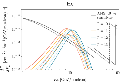
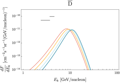
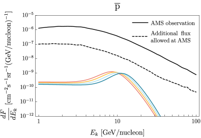
Figure 6: Predicted spectra of anti-nuclei upon propagation to the Earth as a function of kinetic energy per nucleon $E_{k}$, for different choices of the initial Lorentz factor $\Gamma$, as annotated by the different colored lines. The best available sensitivity of AMS to anti-helium (top panel) and anti-deuterium (middle panel) events [67, 68, 69, 70, 71] are presented for comparison in gray (see text). In the top panel, the solid and dashed lines correspond to the isotopes ${}^{3}\overline{\rm He}$ and ${}^{4}\overline{\rm He}$, respectively. The anti-proton flux observed by AMS is shown (bottom panel) by a solid black line [72], while the additional flux required to exceed the uncertainties on the measured flux is shown as the dashed black line in that same panel; fireball production is a negligible source of galactic $\bar{p}$ at these parameter values. Throughout this figure, we fix $\Gamma_{\rm inj}=4\times 10^{35}\,\text{anti-nuclei s}^{-1}$, while the isotopic abundances at the fireball are set by $X_{{\mkern-2.0mu\bar{\mkern 2.0mu\text{D}}}}=5\times 10^{-3}$; see Eqs. (36) and (38).

The expected number of anti-helium events accumulated at AMS over 10 years (at the 95% CL) can be computed using the output spectra from galprop and the published AMS sensitivity to the flux ratio between anti-helium and helium [67, 68]. This is done by recasting the anti-helium acceptance of each energy bin in terms of this $\overline{\text{He}}/\text{He}$ sensitivity in conjunction with published helium data [69], following the procedure outlined in Appendix B of Ref. [15]; see our Appendix G for a brief review. Assuming the number of events follows Poissonian statistics, and allowing for the joint probability of the predicted numbers of ${}^{3}\overline{\text{He}}$ and ${}^{4}\overline{\text{He}}$ to deviate from their AMS-02 tentative observed values within the 68% confidence interval, the $(X_{{\mkern-2.0mu\bar{\mkern 2.0mu\text{D}}}},\Gamma_{\text{inj.}})$ parameter space consistent with the AMS-02 candidate anti-helium events is shown in Fig. 7. Explicitly, we require [73]

$$(\Delta\chi^{2})_{{}^{4}\overline{\text{He}}}+(\Delta\chi^{2})_{{}^{3}\overline{\text{He}}}<2.3\>.$$ (48)

The events for each isotope are assumed to be independent, satisfying

$$(\Delta\chi^{2})_{i}=2\left[N_{i}^{\text{th}}-N_{i}^{\text{obs}}-N_{i}^{\text{obs}}\ln\left(\frac{N_{i}^{\text{th}}}{N_{i}^{\text{obs}}}\right)\right],$$ (49)

where $N_{i}^{\text{th}}$ is the number of events for species $i$ predicted by galprop given a set of model parameters $\{\Gamma_{\text{inj.}},X_{{\mkern-2.0mu\bar{\mkern 2.0mu\text{D}}}}\}$, whereas $N_{i}^{\text{obs}}$ is the fiducial number of candidate $i$ events reported by AMS-02. For the benchmark $X_{{\mkern-2.0mu\bar{\mkern 2.0mu\text{D}}}}=5\times 10^{-3}$ shown by the black dot in Fig. 7, the isotope ratio $N_{{}^{4}\overline{\text{He}}}/N_{{}^{3}\overline{\text{He}}}$ changes from $N_{{}^{4}\overline{\text{He}}}/N_{{}^{3}\overline{\text{He}}}|_{\text{inj.}}\approx 0.33$ at injection to an observed value of $N_{{}^{4}\overline{\text{He}}}/N_{{}^{3}\overline{\text{He}}}|_{\text{obs.}}\approx 0.55$–$0.60$ (depending on the choice of $\Gamma$).

Part of this change in the isotope ratio from injection to observation has to do with physical propagation effects such as spallation of ${}^{4}\overline{\text{He}}$ onto the interstellar medium; however, only $\sim 10$% of the ${}^{3}\overline{\text{He}}$ abundance arises from this effect, which moves the isotopic ratio by only an $\mathcal{O}(1)$ factor. Moreover, that effect would tend to drive the ratio in the other direction (i.e., it reduces ${}^{4}\overline{\text{He}}$ and increases ${}^{3}\overline{\text{He}}$). The larger part of the change arises not from propagation effects at all, but rather from the fact that the AMS-02 anti-helium sensitivity, which we take to be given as the same function of rigidity $\mathcal{R}$ for all anti-helium isotopes (see Appendix G), is not flat as a function of $\mathcal{R}$; on the other hand, the post-propagation energy-per-nucleon spectra of ${}^{3}\overline{\text{He}}$ and ${}^{4}\overline{\text{He}}$ are almost the same (since they have the same energy-per-nucleon at injection), resulting in rigidity distributions for the two species that peak at different values of $\mathcal{R}=(m/Q)\sqrt{(E/m)^{2}-1}$ (i.e., when stated in terms of the kinetic energy per nucleon, the AMS-02 sensitivity that we assume differs for species with different charge-to-mass ratios; see the top panel of Fig. 6). Ultimately, however, this $\mathcal{O}(2)$-factor change could easily be absorbed into a slightly different parameter point if any of the assumptions leading to this effect are found to be inaccurate.

For the case of anti-deuterium, a robust detection relies on the rejection of backgrounds (particularly $\bar{p}$ and He) that are substantially more abundant. As described in Ref. [71], the latest published AMS-02 anti-deuterium sensitivity curve (shown in Fig. 6) is based on an earlier superconducting-magnet configuration for AMS-02, rather than the permanent-magnet configuration actually in use, and cuts off at $\approx 5\,\text{GeV/nucleon}$. Nevertheless, taking that sensitivity, only injections taking place with $\Gamma\lesssim 12$ would result in $\gtrsim 0.1$ expected ${\mkern-2.0mu\bar{\mkern 2.0mu\text{D}}}$ events in the parameter space of interest, but it would be challenging on the basis of that sensitivity to simultaneously account for the 7 candidate anti-deuterium events reported in Ref. [7] in addition to the candidate anti-helium events. That said, an updated study of the AMS-02 anti-deuteron sensitivity would be required to accurately determine whether a single choice of parameters $(X_{{\mkern-2.0mu\bar{\mkern 2.0mu\text{D}}}},\Gamma_{\text{inj.}})$ could achieve this.

Finally, anti-proton events arising from the fireball are also expected to be observed at AMS-02; indeed, as seen in Fig. 6, this flux dominates those of the other species in the parameter regime of interest. However, conventional astrophysical sources are responsible for an anti-proton flux that is greater than that created by the fireballs by a factor of $\sim 10^{3}$ [72]. Producing sufficiently many events to exceed the uncertainty on this measurement (tantalizing in light of the anti-proton excess of $\sim 10\%$ at similar energies [65]) would require a greater anti-nucleus injection rate than is favored by the candidate anti-helium observations; see however Fig. 9 in Appendix B (and related discussion) for an alternative parameter point that may be more interesting from this perspective.

Figure 7: The region of parameter space for which AMS-02 would be expected to observe 3 events of ${}^{4}\overline{\rm He}$ and 6 events of ${}^{3}\overline{\rm He}$ in $T\sim 10$ years, with the injection taking place at $\Gamma=10$. (The allowed region is approximately identical over the range $8.5\leq\Gamma\leq 13$.) The anti-nucleus injection rate $\Gamma_{\rm inj}$ normalizes the total rate of fireball injection of anti-cosmic rays into the MW, whereas the individual source isotopic ratios $X_{i}$ are set by the fireball anti-deuterium abundance $X_{{\mkern-2.0mu\bar{\mkern 2.0mu\text{D}}}}$: $X_{i}=X_{i}(X_{{\mkern-2.0mu\bar{\mkern 2.0mu\text{D}}}})$ via Eqs. (34)–(40). The predicted number of anti-helium events is allowed to independently vary from the fiducial quantity within the 68% confidence interval of the joint probability distribution [see Eq. (48)]. The black dot shows the fiducial parameter values referred to in Fig. 6 and Eq. (55).

IV.2 Other signatures (indirect detection)

In this section, we examine the detectability of X-ray, anti-neutrino, and positron bursts which arise from the fireball model (discussed in Sec. III.3.9). While fireball injection of anti-nuclei is envisaged as a continuous process compared to the galactic dwell-time for these (diffusively transported) particles, the rapid expansion timescale $\tau^{\prime}$ and low galactically-integrated injection event rates $\Gamma_{\text{coll.}}\sim 3\,\text{s}^{-1}$ involved (see Sec. V.1 for this estimate) mean that the non-nuclear outputs from independent fireball injections are temporally well-separated at the Earth and so are best treated independently (with the exception of positrons, whose transport is also diffusive).

At the fluxes required to explain the AMS-02 candidate anti-helium events, there should be $N_{\text{inj.}}\sim\Gamma_{\text{coll.}}T\sim 10^{9}$ events occurring within the galaxy over $T\sim 10\,\text{yr}$. Suppose that we made an observation to look for their non-nuclear products that has a duration $T_{\text{obs.}}$ and that observes a fraction $f_{\text{sky}}$ of the whole sky. In this time, we estimate that the closest observable injection event would occur at a distance $d_{\text{inj.}}\sim 16\,\text{pc}\times(10\,\text{yr}/T_{\text{obs.}})^{1/3}\times f_{\text{sky}}^{-1/3}$ from Earth, if we assume that the injections arise from collisions of the sub-component composite DM states whose benchmark parameters we discuss below in Sec. V.1.

Photons are rapidly released in a burst when the fireball arising from the injection becomes optically thin, at size $R_{\text{thin}}\sim 400\,\text{m}$; see Eq. (45) for this benchmark. We estimate the energy released in this burst to be $\sim g_{*}(T_{\text{thin}}^{\prime})^{4}\Gamma^{2}R_{\text{thin}}^{2}\Delta R_{\text{thin}}\sim g_{*}(T^{\prime}_{\text{thin}})^{4}R_{\text{thin}}^{3}\sim 6\times 10^{27}\,\text{erg}$ [using the benchmark at Eq. (45), and $g_{*}\sim 2$], which results in the emission of $N_{\gamma}\sim 6\times 10^{35}$ photons with average energy $\Gamma T^{\prime}_{\text{thin}}\sim 7\,\mathinner{\mathrm{keV}}$. X-ray telescopes sensitive to such events have an effective area $A_{\gamma}\sim 1000\,\text{cm}^{2}$ [74, 75], a field of view of at most $\Omega_{\gamma}\sim 100$ square degrees (i.e., $f_{\text{sky}}\sim 2\times 10^{-3}$), and mission lifetimes of $\mathcal{O}(\text{years})$. The total expected number of photons arriving at the detector from the closest release that would occur would be $\sim N_{\gamma}(A_{\gamma}/d_{\text{inj.}}^{2})\sim 0.2\times f_{\text{sky}}^{2/3}\times(T_{\text{obs.}}/10\,\text{yr})^{2/3}$. Even if we conservatively ignore the finite field of view (i.e., set $f_{\text{sky}}\sim 1$) and take $T_{\text{obs.}}\sim 10\,\text{yr}$, this is too faint to observe. There may additionally be a diffuse background of X-ray photons due to the cumulative injections taking both intra- and extra-galactically over extended periods of time, but we have not estimated this here.

Anti-neutrinos may be injected promptly when the fireball thermalizes, or indirectly through the decay of injected pions. The fraction of the total energy $g_{*}T_{0}^{4}R_{0}^{3}\sim 4\times 10^{32}\,\text{erg}$ [see Eq. (43) for this benchmark; we set $g_{*}\sim 5.5$] that is carried by the prompt anti-neutrinos is $\sim G_{F}^{2}T_{0}^{5}\tau^{\prime}\sim 1\%$ (for $\tau^{\prime}\sim R_{0}$ as at early times; see Fig. 1), corresponding to $N_{\nu,\,\text{scatter}}\sim 3\times 10^{34}$ particles with an average energy of $T_{0}\sim 100\,\mathinner{\mathrm{MeV}}$. As far as (anti-)neutrinos from decay are concerned, thermal pions have a number density $n_{\pi}\sim(m_{\pi}T/(2\pi))^{3/2}\exp(-m_{\pi}/T)$ within the fireball, so the number of neutrinos injected due to their decay is $N_{\nu,\,\text{decay}}\sim n_{\pi}R^{3}(\tau^{\prime}/\tau_{\pi})\lesssim 10^{31}$, where $\tau_{\pi}\sim 10^{-8}\,\text{s}$ is the charged pion lifetime. Their average energy is also $\sim\Gamma(m_{\pi}-m_{\mu})\sim 100\text{ MeV}$. The decay contribution is thus sub-dominant. Given a neutrino detector in this energy range, with an area $A_{\nu}\sim(100\,\text{m})^{2}$ [76], roughly $\sim N_{\nu}A_{\nu}/(d_{\text{inj.}})^{2}\sim 10^{3}\times(T_{\text{obs.}}/10\,\text{yr})^{2/3}$ neutrinos would pass through the detector as a result of the nearest injection in the observation time. The probability of a single neutrino interacting in the detector is $p_{\nu}\sim n_{T}G_{F}^{2}E_{\nu}^{2}d_{T}$ where $n_{T}\sim 3\times 10^{22}/\text{cm}^{3}$ is the target (e.g., water [76]) number density, and $d_{T}$ is the target thickness. Taking $E_{\nu}\sim 100\,\mathinner{\mathrm{MeV}}$ and $d_{T}\sim 100\,\text{m}$ as relevant for our assumptions, we find $p_{\nu}\sim 10^{-13}$, so the expected number of detectable events is $\sim 10^{-10}\times(T_{\text{obs.}}/10\,\text{yr})^{2/3}\ll 1$ for any conceivable observation duration.

Positrons injected by the fireball are potentially observable in two ways: directly as cosmic rays, and indirectly through $511\,\text{keV}$ photons produced when they annihilate with electrons in the ISM. However, the injected positron energies are $\sim\Gamma m_{e}\sim 10\,\text{MeV}$, which falls below the AMS-02 sensitivity threshold (even without accounting for further energy loss during propagation), likely making them unobservable. For the 511 keV emission, the total integrated positron injection rate from fireballs cannot exceed the total integrated anti-baryon injection rate (cf. the discussion about $X_{Q}<0$ in Appendix B), which from the numbers shown in Fig. 7 is maximally $\Gamma_{\text{inj.}}\sim(\text{few})\times 10^{36}\,\text{s}^{-1}$; this is much smaller than the integrated positron injection rate of $\sim 10^{43}\,\text{s}^{-1}$ that explains 511 keV emission in the MW [89]. The fireball-injected positrons annihilating therefore likely only contributes a sub-dominant 511 keV flux.

On the basis of these estimates, these non-nuclear products thus do not appear to be observable; however, a more detailed investigation of these (indirect-detection) signatures of this class of models may be worthwhile in future work.

V A dark-matter origin for the fireballs?

Thus far, we have operated under the assumption that a rapid, localized injection of energetic Standard Model anti-baryons can be achieved in order to seed the fireballs. A BSM mechanism is required to explain these injections.

In this section, we discuss whether the collisions of large, composite dark-matter states that carry anti-baryon number may be able to provide such a mechanism. Assuming that a substantial fraction of the mass energy of such colliding DM states can be promptly converted to SM anti-quarks as a result of dynamics triggered by the collision, we demonstrate in Sec. V.1 that the requisite injection rate of anti-baryon number could be achieved for DM states with certain bulk physical properties (i.e., total mass, number of constituents, and physical size). In Sec. V.2 we then show that, provided certain benchmarks can be realized in the conversion of the dark-state mass energy to the SM, fireballs with appropriate bulk parameters $(T_{0},R_{0},\bar{\eta})$ could also be seeded. As this is suggestive, in Sec. V.3 we then advance some speculations toward specific microphysical DM models in which we suspect this could possibly occur. We emphasize, however, that we have not settled the question of whether one or more of these models actually do in fact realize the required dynamics. While we intend to return to this open question in future work, we also encourage other work on this point.

V.1 Collision rates

Suppose that a fraction $0<f_{\textsc{dm}}\leq 1$ of the DM energy density is comprised of large, cosmologically stable composite objects. The existence, formation, and signatures (or lack thereof) of a variety of objects of this type have been subjects of extensive study in the literature [90, 91, 92, 93, 94, 95, 96, 97, 98, 99, 100, 101, 102, 103, 104, 105, 106, 107, 108, 109, 110] (see also Refs. [111, 112]). For the purposes of the estimate we give here, we assume that these objects have a mass dominated by $N_{\textsc{dm}}$ constituents, each with mass $m_{\textsc{dm}}$ and baryon number of $-1$, giving them a total mass $M_{\textsc{dm}}\sim N_{\textsc{dm}}m_{\textsc{dm}}$ and total baryon number $B_{\textsc{dm}}=-N_{\textsc{dm}}$; we take their radius to be $R_{\textsc{dm}}$.

Taking a collision cross-section

$$\sigma\sim\pi R_{\textsc{dm}}^{2}\Sigma\>,$$ (50)

where $\Sigma\geq 1$ is a Sommerfeld-like enhancement to the geometrical cross-section, the collision rate of two such blobs integrated over the whole $V_{\textsc{mw}}=40\times 40\times 11\,\text{kpc}^{3}$ simulation volume used in galprop (see Sec. IV.1), can be estimated as

$$\Gamma_{\text{coll.}} \sim\int dV\left(\frac{f_{\textsc{dm}}\rho_{\textsc{dm}}(r)}{M_{\textsc{dm}}}\right)^{2}(\pi R_{\textsc{dm}}^{2}\Sigma)v_{\textsc{dm}}$$ (51)

$$\equiv V_{\textsc{mw}}\left(\frac{f_{\textsc{dm}}\rho_{0}}{M_{\textsc{dm}}}\right)^{2}(\pi R_{\textsc{dm}}^{2}\Sigma)v_{\textsc{dm}}\times\mathcal{I}_{\textsc{dm}}^{\textsc{mw}}$$ (52)

$$\sim 3\,\text{s}^{-1}\times\left(\frac{f_{\textsc{dm}}}{0.01}\right)^{2}\left(\frac{\Sigma}{1}\right)$$

$$\qquad\times\left(\frac{N_{\textsc{dm}}}{5\times 10^{36}}\right)^{-2}\left(\frac{m_{\textsc{dm}}}{10\,\mathinner{\mathrm{GeV}}}\right)^{-2}\left(\frac{R_{\textsc{dm}}}{1\,\text{m}}\right)^{2}.$$ (53)

At Eq. (51), $\rho_{\textsc{dm}}(r)$ is the DM energy density at galactocentric radius $r$, as specified in the NFW model [116] (see Sec. IV.1), and $v_{\textsc{dm}}\sim 10^{-3}$ is the typical velocity of blobs in the galaxy (we take this to be constant over $r$). At Eq. (52), we have have defined $\mathcal{I}_{\textsc{dm}}^{\textsc{mw}}\equiv\int(dV/V_{\textsc{mw}})\left[\rho_{\textsc{dm}}(r)/\rho_{0}\right]^{2}\approx 0.85.$

In the above numerical estimate, we considered benchmark blobs with radius $R_{\textsc{dm}}\sim 1\,\text{m}$, number of constituents $N_{\textsc{dm}}\sim 5\times 10^{36}$, and constituent mass $10\,\mathinner{\mathrm{GeV}}$, giving a total blob mass of $M_{\textsc{dm}}\sim 9\times 10^{10}\,\text{kg}$ (roughly the mass of a typical Main Belt asteroid with a diameter of a few-hundred meters) and an average density $\sim 2\times 10^{7}\,\text{g/cm}^{3}$ (while much more dense than ordinary matter, this is still less dense than a non-extremal SM white dwarf). We have also assumed that they constitute only about $\sim 10$% of the DM, and have conservatively neglected any Sommerfeld-like enhancement to the collisions rate.

We assume further that, upon such pair-wise collisions, the DM states can be destabilized in such a way that a fraction $0<f_{\textsc{sm}}\leq 1$ of their combined number of constituents is converted to Standard Model anti-quarks, seeding into the SM a total baryon number $B_{\text{inj.}}=-2f_{\textsc{sm}}N_{\textsc{dm}}$ per collision. The injection rate of anti-baryon number (cf. Fig. 7) can then be estimated as

$$\Gamma_{\text{inj.}} \sim|B_{\text{inj.}}|\Gamma_{\text{coll.}}$$ (54)

$$\sim 4\times 10^{35}\,\text{s}^{-1}\times\left(\frac{f_{\textsc{sm}}}{1.5\times 10^{-2}}\right)\left(\frac{f_{\textsc{dm}}}{0.01}\right)^{2}\left(\frac{\Sigma}{1}\right)$$

$$\qquad\times\left(\frac{N_{\textsc{dm}}}{5\times 10^{36}}\right)^{-1}\left(\frac{m_{\textsc{dm}}}{10\,\mathinner{\mathrm{GeV}}}\right)^{-2}\left(\frac{R_{\textsc{dm}}}{1\,\text{m}}\right)^{2}.$$ (55)

Importantly, for these benchmark bulk DM parameters, we find that this could achieve the injection luminosity required to obtain the correct fiducial number of candidate anti-helium events at AMS-02, $\Gamma_{\text{inj.}}\sim 4\times 10^{35}\,\text{s}^{-1}$ (cf. Fig. 7), for $f_{\textsc{sm}}f_{\textsc{dm}}^{2}\Sigma\sim 10^{-6}$. That is, the requisite injection rate could be achieved even with large composite DM that is a sub-component of the total DM density and that is not very efficient in converting constituent anti-baryon number to SM anti-quarks upon collision, all without any Sommerfeld-like enhancement to the collision rate. Of course, these conclusions change for different DM bulk parameter ranges, per Eq. (55).

Note also that the typical inter-collision time here, $1/\Gamma_{\text{coll.}}\sim 0.4\,\text{s}$, is $\sim 14$ orders of magnitude shorter than the diffusion time $t_{\text{diff}}\sim 10^{6}\,\text{yr}$ for the charged cosmic rays to escape the MW [65], which also justifies a posteriori treating the injection as a roughly constant-in-time source term in galprop (see Sec. IV.1).

V.2 Mapping to fireball parameters

While we cannot robustly estimate the fireball parameters $(T_{0},R_{0},\bar{\eta})$ that would obtain from such collisions without a model, we can show that these dark composite DM states would be able, at the order of magnitude level, to generate approximately the benchmark fireball parameters discussed at Eq. (43).

If we assume that $f_{\textsc{sm}}$ is also the fraction of energy injected into the SM anti-quarks, then the energy injected is $E_{\text{inj.}}\sim m_{\textsc{dm}}|B_{\text{inj.}}|$. If we take $T_{0}\lesssim 100\,\mathinner{\mathrm{MeV}}$ (verified a posteriori), this energy must go to the mass-energy of $|B_{\text{inj.}}|$ anti-nucleons (they dominate the fireball anti-baryonic output) and the remainder to $g_{*}\sim 5.5$ relativistic species. That is, $E_{\text{inj.}}\sim m_{\textsc{dm}}|B_{\text{inj.}}|\sim m_{p}|B_{\text{inj.}}|+g_{*}(\pi^{2}T_{0}^{4}/15)(4\pi R_{0}^{3}/3)$. Therefore,

$$T_{0} \sim\left[\frac{45f_{\textsc{sm}}}{2\pi^{3}g_{*}}(m_{\textsc{dm}}-m_{p})\frac{N_{\textsc{dm}}}{R_{0}^{3}}\right]^{1/4}$$ (56)

$$\sim 62\,\mathinner{\mathrm{MeV}}\times\left(\frac{f_{\textsc{sm}}}{1.5\times 10^{-2}}\right)^{1/4}\left(\frac{g_{*}}{5.5}\right)^{-1/4}$$

$$\qquad\times\left(\frac{N_{\textsc{dm}}}{5\times 10^{36}}\right)^{1/4}\left(\frac{R_{0}}{3.6\,\text{mm}}\right)^{-3/4}$$

$$\qquad\times\left(\frac{m_{\textsc{dm}}-m_{p}}{10\,\mathinner{\mathrm{GeV}}-m_{p}}\right)^{1/4}\>,$$ (57)

where we have assumed that the fireball injection happens in a region of radius $R_{*}$ that is much smaller than $R_{\textsc{dm}}$ (i.e., $R_{*}\sim R_{0}\ll R_{\textsc{dm}}$), consistent with that injection occurring as a result of some catastrophic collapse dynamics in the post-collisional evolution (see Sec. V.3).

Meanwhile, in the final post-fireball evolution, we have roughly that $E_{\text{inj.}}\sim\Gamma m_{p}|B_{\text{inj.}}|$, so $\Gamma\sim m_{\textsc{dm}}/m_{p}\sim 11\times(m_{\textsc{dm}}/10\,\mathinner{\mathrm{GeV}})$, corresponding to $\bar{\eta}\sim 6.1\times 10^{-3}$. Moreover, the constant $c$ defined at Eq. (42) is $c\sim 1.24$, implying an injected anti-helium isotope ratio of $N_{{}^{4}\overline{\text{He}}}/N_{{}^{3}\overline{\text{He}}}|_{\text{inj.}}\sim 0.33$, roughly consistent with an observed isotope ratio of $N_{{}^{4}\overline{\text{He}}}/N_{{}^{3}\overline{\text{He}}}|_{\text{obs.}}\sim 0.5$, as discussed in Sec. IV.

In order the achieve the requisite net negative charge on the hadronic sector of the fireball in order to obtain a value $X_{\bar{p}}\sim 0.5$ around the onset of anti-nucleosynthesis (see the discussion in Sec. III.3.3 and Appendix B) while also maintaining net fireball EM neutrality (as required for injections from net-neutral dark objects), it would be sufficient for the injection to take place in such a way that a fraction $X_{p}$ of the anti-baryons are anti-protons, with a corresponding number $L\sim X_{p}|B_{\text{inj.}}|$ of positively charged leptons being injected. On energetics grounds, because $m_{e}\ll m_{p}$ and $f_{\textsc{sm}}\ll 1$, this can easily be accomplished with minimal change to the above discussion. It would however require the initial dark object to carry net-negative lepton number in addition to net-negative baryon number.

While the precise values shown in both this subsection and the previous one should not be taken too literally given the roughness of the estimates, what this nevertheless indicates is that collisions of large, macroscopic dark objects can in principle attain both the requisite injection rates and required fireball conditions to make our anti-helium anti-nucleosynthesis mechanism operate in a phenomenologically viable fashion, provided that the benchmarks and broad model features we have given can be attained in a concrete model.

V.3 Towards a particle physics model

The development a detailed microphysical model for the composite dark states, and their evolution in and after collisions is a question we ultimately leave open in this paper. Nevertheless, in this section, we sketch the outlines of two particle physics models that we believe are promising targets for future investigation, and indicate where the difficulties in understanding their evolution lie. We intend to return to this point in future work, and also encourage other work on it.

V.3.1 Imploding fermion+Yukawa model

The requisite injection may result from rapid conversions of $N_{\chi}\sim|B_{\text{inj.}}|/q_{B}$ fundamental DM particles $\chi$, each carrying baryon number $-q_{B}$ ($q_{B}>0)$ [and possibly lepton number], into SM anti-particles via a higher-dimensional effective operator; e.g., something of the form $\bar{\chi}\bar{\chi}\bar{\chi}\bar{q}\bar{q}\bar{q}$ if only anti-baryon number needs to be injected, or something like $\bar{\chi}\bar{\chi}\bar{\chi}\bar{\chi}\bar{q}\bar{q}\bar{q}\bar{\ell}$ if both anti-baryon and anti-lepton number need to be injected primarily (here, $\bar{q}$ and $\bar{\ell}$ represent an anti-quark and anti-lepton, respectively); see discussions in Secs. III.1 and III.3.3, and Appendix B.

Simultaneous and spatially concentrated conversions of a large number of $\chi$ particles can be naturally achieved if the $\chi$ particles participating in the conversion existed in the form of blobs; i.e., large composite bound states. While these blobs, presumably formed in the early Universe, must survive over $\sim 10\,\text{Gyr}$ timescale until the present epoch, they must also rapidly convert to anti-quarks in $\sim 10^{-12}\,\text{s}$ timescale when the time is ripe (within the last $\sim\text{Myr}$ timescale for anti-nuclei to escape the Galaxy). To bridge these extremely long and extremely short timescales required for the DM$\rightarrow$SM process, we can imagine the following scenario. These blobs may have existed in a metastable state in the sense that they are individually stable, with the rate of the DM$\rightarrow$SM conversion process within each blob satisfying $\Gamma_{\text{DM}\rightarrow\text{SM}}\ll(10\,\text{Gyr})^{-1}$, but the merger of a pair of blobs would trigger a runaway collapse of the merger product accompanied with many orders of magnitude increase in $\Gamma_{\text{DM}\rightarrow\text{SM}}$, eventually causing most of the $\chi$ particles to convert to SM anti-particles when $1/\Gamma_{\text{DM}\rightarrow\text{SM}}\sim 10^{-12}\,\text{s}$.

The stable blob can be kept in equilibrium, for instance, by the balance between the repulsive effect of the Fermi pressure of $\chi$ particles and the compressing effect due to a higher vacuum pressure outside compared to inside the blob. Such a vacuum pressure difference $P_{\rm vac}^{\rm out}-P_{\rm vac}^{\rm in}>0$ arises naturally in scenarios where the blobs are formed through a cosmological first-order phase transition from a higher-energy false vacuum to a lower-energy true vacuum in the early Universe [101, 90, 99, 102, 112, 111]. In those scenarios, the present-epoch setup is that the inside of the blobs remains in the false vacuum while the rest of the Universe is in the true vacuum. Correspondingly, the pressure $P_{\rm vac}=-\rho_{\rm vac}$ associated with the vacuum energy $\rho_{\rm vac}$ is more negative inside than outside the blob.

Runaway collapse can be achieved by incorporating additional Yukawa forces between $\chi$ particles with an intermediate-range mediator: long compared to the typical spacing between $\chi$ but short compared to the radius of the blob. We additionally assume that the $\chi$ are non-relativistic to avoid suppressions in their Yukawa forces (cf. Refs. [93, 95] and the discussion in the next subsection). The total Fermi kinetic energy of the blob, the vacuum energy difference between inside and outside the blob, and the attractive Yukawa potential for an intermediate-range mediator then scale with the blob’s number of constituents $N_{\chi}$ and radius $R_{\rm blob}$ as $\propto N_{\chi}^{5/3}/R_{\rm blob}^{2}$, $\propto R_{\rm blob}^{3}$, and $\propto-N_{\chi}^{2}/R_{\rm blob}^{3}$, respectively. For a given sufficiently small $N_{\chi}$, the blob’s total energy as a function of $R_{\rm blob}$ has a metastable minimum at a radius that is set by the balance between the non-relativistic Fermi pressure and vacuum-pressure difference. However, when $N_{\chi}$ exceeds a certain threshold the metastable minimum ceases to exist and it becomes energetically favorable for $R_{\rm blob}$ to decrease indefinitely, until new effects that deplete the $\chi$ or reverse the tendency to collapse turns on. Such a runaway collapse can be triggered by the merger of two near-critical blobs.

Aside from the complexity of accurately modeling the envisaged scenario, one can already see competing effects or constraints that make it challenging to present a concrete realization of this scenario. First, the requirement to reduce the blob radius by many orders of magnitude during the blob collapse in order to increase $\Gamma_{\text{DM}\rightarrow\text{SM}}$ from $\ll(10\,\text{Gyr})^{-1}$ to $\sim(10^{-12}\,\text{s})^{-1}$ can increase the Fermi momentum of the $\chi$ particles to the point that they become relativistic. Once the $\chi$ particles are relativistic, the Yukawa forces become progressively suppressed [93, 95] and at the same time the Fermi pressure increases faster as the blob radius decreases [117]. Both these effects tend to stop the collapse, potentially preventing $\Gamma_{\text{DM}\rightarrow\text{SM}}$ from reaching $\sim(10^{-12}\,\text{s})^{-1}$. Moreover, consistency with collider data (and $\tilde{E}|_{\text{inj.}}/\tilde{B}|_{\text{inj.}}\sim 10\,\mathinner{\mathrm{GeV}}$ to obtain $\Gamma\sim 10$) requires raising the cutoff of the higher-dimensional DM$\rightarrow$SM operator to at least above $10\,\mathinner{\mathrm{TeV}}$. The latter implies a strong suppression on $\Gamma_{\text{DM}\rightarrow\text{SM}}$ unless the blob becomes very dense at the time of conversion. Preliminary estimates suggest that in order to obtain $1/\Gamma_{\text{DM}\rightarrow\text{SM}}\sim 10^{-12}\,\text{s}$, the energy density of the blob at the time of conversion must be $\gg(100\,\mathinner{\mathrm{MeV}})^{4}$, which is much higher than the typical energy density of the fireball we seek to create. To dilute such a high energy density one may need to introduce another operator that converts the $\chi$ particles to a lighter dark particles $\psi$ much more efficiently than the DM$\rightarrow$SM conversion, such that most of the $\chi$ convert into $\psi$ with a rate $\Gamma_{\chi\rightarrow\psi}\sim(10^{-12}\,\text{s})^{-1}$, and only a small fraction $f_{\rm SM}\sim 10^{-12}\,\text{s}\times\Gamma_{\text{DM}\rightarrow\text{SM}}\ll 1$ of $\chi$ with energy density $\sim(100\,\mathinner{\mathrm{MeV}})^{4}$ converts to SM anti-particles during the $\sim 10^{-12}\,\text{s}$ timescale.

V.3.2 Dark-dwarf model

The second model that we believe may be interesting to consider is based on the dark states behaving somewhat like white dwarfs in the SM. The particle content of this model would be a heavy “dark proton” $p_{d}$, a slightly heavier “dark neutron” $n_{d}$, a much lighter “dark electron” $e_{d}$, and a massless “dark neutrino” $\nu_{d}$. The $p_{d}$ and $n_{d}$ carry baryon number $-1$, and both couple with equal strength to a Yukawa force mediated by a scalar $\varphi$. Additionally, the $p_{d}$ and $e_{d}$ are taken to both couple to a dark electromagnetism, with opposite charges. We also assume the existence of a two higher dimensional 4-fermion operators allowing $e_{d}+p_{d}\leftrightarrow n_{d}+\nu_{d}$ (and crossed) reactions, and permitting $n_{d}\rightarrow\bar{q}+\bar{q}+\bar{q}$, where $\bar{q}$ is a SM anti-quark.

With such particle content, it is possible to form dense macroscopic composite objects (“dark dwarfs” [102]) with very large constituent number, consisting of $p_{d}$ held together by the Yukawa force, and supported against collapse by the (relativistic) degeneracy pressure of the $e_{d}$. The mass hierarchies of the particles can be arranged such that, at zero temperature, these objects would initially contain no $n_{d}$ or $\nu_{d}$ constituents.

Similar objects, albeit with just a single uncharged constituent fermion supported against collapse due to attractive Yukawa forces by its own degeneracy pressure, have been considered in, e.g., Refs. [92, 93, 95, 98]; see also Ref. [102]. A straightforward extension of these works to the two-component dark dwarf we have in mind indicates that these objects, while not possessing a singular collapse instability (i.e., there is no true Chandrasekhar-like limit), possess of threshold constituent number $N_{*}$ for which the following is true: for $0<N<N_{*}$, their radii $R$ are large, say $R\sim R_{\text{below}}$; on the other hand, for $N_{*}<N<2N_{*}$, their radii $R\sim R_{\text{above}}$ are much smaller. Roughly, the hierarchy of these radii is in ratio of the dark electron and proton masses: $R_{\text{above}}\sim(m_{e_{d}}/m_{p_{d}})R_{\text{below}}\ll R_{\text{below}}$.

If the cosmologically stable dark objects have $N_{\textsc{dm}}\sim\epsilon N_{*}$ with $0.5\lesssim\epsilon<1$, then collisions of two such objects could in principle trigger a large change in the bulk properties of the pre- and post-collision states because (assuming no ejection of constituents), the post-collision object would than have $N\sim 2\epsilon N_{*}>N_{*}$ constituents. If the collision were to play out in such a way that both the pre- and post-collision states were at exactly zero (dark) temperature, the idea would heuristically be the following: before collision, the Fermi energy of the (relativistic) $e_{d}$ is much smaller than the mass difference of the $n_{d}$ and $p_{d}$. However, when these objects collide and then dynamically relax down to their much smaller post-collision equilibrium size, the $e_{d}$ density increases greatly, leading to their Fermi energy becoming much larger. Once the $e_{d}$ Fermi energy exceeds the $n_{d}$–$p_{d}$ mass difference, a large fraction of the $p_{d}$ can suddenly “neutronise” to $n_{d}$ (we adopt the nomenclature of the cognate process that occurs in the collapse toward a SM neutron star [117]). The $n_{d}$ in turn are unstable to decay to SM anti-quarks. As a result, the sudden dynamical “collapse” of the incoming dark states to a much smaller and more dense state upon collisions could trigger a catastrophic decay of a large fraction of the mass energy of the initial colliding dark objects to SM anti-quarks.

Unfortunately, the dynamics of this system are actually more complicated than this naïve picture. Initial estimates indicate that for scalar forces with a range larger than the blob sizes (the regime we assume), there is a speed up of the dark states as they collide, leading to the collision taking place in a supersonic regime with respect to the estimated speed of sound in the blobs. As a result, two things are true: (1) the collision is a violent process that is not amenable to simple analytical treatment, and could lead to the ejection of constituents, or the formation of a large bound object, or (more likely) something more complicated; and (2) as the collision occurs, it is likely that the blob constituents are heated significantly (via, e.g., shock heating), possibly to initial post-collision dark temperatures $T_{d}$ that are a significant fraction of the dark electron mass $m_{e_{d}}$. As a result, the zero-temperature dynamics of the object are likely significantly modified by resulting thermal pressures. It appears that the resulting state may still lose energy and shrink via surface dark-photon emission, volume relativistic emission of the $\varphi$ particle, and later potentially either volume or surface emission of dark neutrinos. The resulting state may thus still evolve toward the neutronization regime sufficiently rapidly for this model to be viable. However, the entirety of this evolution is complicated and requires further study to establish in detail whether it works.

While this model may potentially be able to achieve the requisite destabilization dynamics, obtaining a net-negative EM charge on the anti-hadrons for fireballs seeded by this model (see discussions in Secs. III.3.3 and V.2, and Appendix B) may be challenging in the exact formulation advanced here. A modification to this picture, or further model building, may be required.

The scope of work required to investigate this model in full and place the speculative statements in this sub-section on a firm footing is such that we defer its consideration to a future paper.

VI Discussion and conclusion

In this paper we have studied the anti-nucleosynthesis of elements up to anti-helium-4 in rapidly expanding fireballs of SM plasma that carry net anti-baryon number and that we assume to be seeded within the Milky Way by a BSM process. For appropriate initial conditions set by the initial radius, temperature, and anti-baryon–to-entropy ratio of the plasma, the evolution of these fireballs is such that their thermal pressure drives the system toward a regime where there is relativistic bulk radial motion of a thin shell of plasma, in which the temperature of plasma falls as the expansion proceeds. This permits purely SM thermal anti-nucleosynthesis of elements (similar to BBN) to occur in the expanding, cooling thin shell, while the products obtain relativistic boosts with respect to the rest frame of the fireball. Eventually, for appropriate parameters, the expansion rate shuts off the anti-nucleosynthesis in a regime where the anti-nucleosynthetic products have not reached their thermodynamic equilibrium values, which allows the abundances of ${}^{4}\overline{\text{He}}$ and anti-tritium (which later decays to ${}^{3}\overline{\text{He}}$) produced to not be too dissimilar, and not highly suppressed with respect to anti-deuterium or anti-protons; see Figs. 3–5. Once this expanding fireball becomes optically thin, its products cease to be driven by thermal pressures, and are launched at relativistic speeds into interstellar space, all with the same bulk speed (i.e., Lorentz boost). The anti-tritium subsequently decays to ${}^{3}\overline{\text{He}}$ on a short timescale, leading to injected amounts of ${}^{3}\overline{\text{He}}$ and ${}^{4}\overline{\text{He}}$ that are not too dissimilar.

Assuming that these injections of high-energy anti-nucleons and anti-nuclei are spatially distributed as the square of an NFW profile, and making use of galprop to approximate the galactic transport of these injected products, we showed that the relative fluxes received at Earth are such that one could obtain a ratio of roughly 2:1 for the isotopes ${}^{3}\overline{\text{He}}$ to ${}^{4}\overline{\text{He}}$, without being excluded by AMS-02 anti-deuterium or anti-proton constraints; see Figs. 6 and 7. We showed that other products of this scenario (e.g., photons) do not appear to supply additional constraints, but we did not undertake an exhaustive indirect detection study. We also computed the overall required injection luminosity of anti-baryons into the fireballs we considered in order to obtain $\mathcal{O}(10)$ anti-helium events in the AMS-02 10-year exposure.

Our conclusion that the sizes of the anti-proton (larger) and anti-helium (smaller) fluxes are not too dissimilar so as to violate observational constraints on the anti-proton flux, while also explaining the anti-helium isotope ratio, does depend to some extent what the anti-proton–to–anti-neutron ratio is in the partially thermalized fireball plasma prior to the onset of anti-nucleosynthesis. Because weak interactions are inefficient in the plasma and weak decay timescales for the charged pions are long compared to the dynamical expansion timescale of the fluid, this value is however dependent on the details of the BSM injection process that seeds the fireball.

In reaching our conclusions as stated above in the main text, we assumed that the charged pions have a small chemical potential (i.e., $|\mu_{\pi^{+}}|\ll m_{n}-m_{p}$) until SMCER reactions such as $\bar{n}+\pi^{-}\leftrightarrow\bar{p}+\pi^{0}$ became inefficient, locking in the $\bar{n}$–to–$\bar{p}$ ratio. This was equivalent to assuming that some combination of the BSM injection and possible SM processes following it were such that they established a certain very specific overall net negative electromagnetic charge (i.e., $X_{Q}=-(n_{Q}^{\prime})^{\text{hadron}}/n_{\bar{B}}^{\prime}>0$; see Appendix B) on the (anti-)hadronic constituents of the fireball no later than the time at which the SMCER begin to be inefficient, with a compensating overall positive charge held by charged leptons in order to allow overall neutrality. But we also showed in Appendix B that we could relax this assumption on the small pion chemical potential somewhat, which allows $X_{Q}$ to vary in some range around 0.5 with only $\mathcal{O}(1)$ changes to our results. However, if $X_{Q}$ is too small around the time the SMCER reactions become inefficient, a larger anti-proton abundance results for the same anti-helium flux, which can be observationally challenging. While we argue that SM processes impose $X_{Q}\gtrsim 5\times 10^{-5}$, we found that $X_{Q}\gtrsim 10^{-2}$ is likely required for phenomenological viability (see Fig. 9). Realizing this thus likely requires that the BSM injection process needs to be able to primarily inject both anti-quarks and anti-leptons of compensating charge.

Finally, we showed that it would be plausible (at least in principle) for the required injection luminosity to be obtained via the collisions of supermassive, composite dark states (possibly a subcomponent of the dark matter), provided that these otherwise individually cosmologically stable states can become destabilized in the collision in such a way that activates a decay channel that converts a non-negligible fraction of their mass energy to SM anti-quarks (and possibly some fraction of positively charged leptons), with this taking place both rapidly and in a localized region of space. We also showed that, assuming certain benchmark bulk behavior in the post-collisional evolution can be realized, this same scenario could seed fireballs with the correct bulk physical values $(T_{0},R_{0},\bar{\eta})$ to realize anti-nucleosynthesis scenario we advance in a phenomenologically viable fashion.

We did not supply a full particle physics model that could computably realize the required behavior, but we offered two potential model paradigms for these dark objects that we believe may be interesting to investigate further in future work. The first paradigm is based on a model with a single species of fermions held together by a combination of vacuum pressure differences inside and outside a large agglomeration of such objects, and an intermediate-range Yukawa force, but supported against collapse by their nonrelativistic degeneracy pressure. Collisions of pairs of such objects may in certain regimes provoke a catastrophic collapse of the resulting combined state if it exceeds a critical threshold of constituents. We can imagine operators that allow some number of these fermions to then mutually annihilate to a collection of SM anti-quarks; modified versions of this behavior could likely realize the opposite-sign lepton injection too. The dramatic density difference in the pre- and post-collision states of these objects may allow them to be cosmologically stable before collision, but for the annihilation rates to spike high enough during the collapse to permit the requisite injection in a sufficiently rapid timescale. The second paradigm is a based on a collision of dark analogues of degenerate white dwarfs, that may undergo rapid collapse after collision, provided the collision produces a merger product above a certain threshold number of constituents. During this collapse, constituents of the dark dwarfs may be converted to other dark species that are unstable to prompt decay to SM anti-quarks. In this case, additional model building or a modification of the picture we presented are likely required to achieve the opposite-charge lepton injection. Neither of these scenarios is however amenable to full analytical control, and important aspects of the evolution of each are thus still unclear.

To be completely clear: it is thus still an open question whether, and how, the requisite BSM injection of SM anti-quarks (and opposite-sign charged leptons) can be achieved via dark-state collisions in order to seed the fireballs whose post-injection SM behavior we have studied. The most obvious and pressing follow-up is therefore a fuller investigation of these (or other) model paradigms, so as to place this BSM aspect of our scenario on a rigorous footing. We anticipate returning to this point in future work.

On the observational side, further AMS-02 data will continue to be taken until 2030 [7]; combined with the existing data, this may yield further clarity about the status of the AMS-02 candidate anti-helium events. Additionally, the balloon-borne GAPS experiment [118] is approved to fly in late-2024 [119], and is anticipated to provide data on lower-energy anti-deuterium and anti-helium fluxes that will be complementary to those from AMS-02. These data will continue to inform model-building.

The fireball anti-nucleosynthesis scenario we have advanced in this paper provides an interesting and novel alternative SM pathway to anti-helium formation, provided that the BSM seeding issue can be appropriately addressed. We therefore view this work a partial step toward understanding the origin of the tentatively identified AMS-02 anti-helium events.

Appendix A Derivation of fireball scaling laws

As described in Sec. III.2, following a transient and localized injection of energy and anti-baryon number, a thermalized fireball with anti-baryon–to–entropy ratio $\bar{\eta}\ll 1$ is formed. In our parameter space, the fireball immediately accelerates to semirelativistic bulk velocities corresponding to Lorentz factors $\gamma\sim\text{few}$, at which point its radius and temperature are $R_{0}$ and $T_{0}$ respectively, turning into a dense shell with a central underdensity in the process. At the point where the radius of the fireball is $R_{0}$, this shell structure is just beginning to form, and the shell thickness can be taken to be $\sim R_{0}$. The subsequent evolution of the shell is dictated by the following relativistic fluid equations which, respectively, encode conservation of anti-baryon number, momentum, and energy in the comoving fluid frame:

$$\partial_{t}\left[\gamma n_{\bar{B}}^{\prime}\right]+\frac{1}{r^{2}}\partial_{r}\left[r^{2}\gamma vn_{\bar{B}}^{\prime}\right] =0\>,$$ (58)

$$\partial_{t}\left[\gamma^{2}(\rho^{\prime}+p^{\prime})\right]+\frac{1}{r^{2}}\partial_{r}\left[r^{2}\gamma^{2}v\left(\rho^{\prime}+p^{\prime}\right)\right] =\partial_{t}p^{\prime}\>,$$ (59)

$$\partial_{t}\left[\gamma^{2}v(\rho^{\prime}+p^{\prime})\right]+\frac{1}{r^{2}}\partial_{r}\left[r^{2}\gamma^{2}v^{2}\left(\rho^{\prime}+p^{\prime}\right)\right] =-\partial_{r}p^{\prime}\>,$$ (60)

where $r$, $t$, $v$ ($\gamma$), $n_{\bar{B}}^{\prime}$, $\rho^{\prime}$, and $p^{\prime}$ are, respectively, the radial position, time, bulk velocity (and its associated Lorentz factor), anti-baryon number density, energy density, and pressure of a fluid element in the fireball. Primed quantities are defined in the comoving rest frame of the fireball fluid; unprimed quantities are defined in the fireball CoM frame.

In this Appendix we show how, in the ultra-relativistic bulk velocity limit $\gamma\gg 1$, the fireball expansion follows the simple scaling laws used Sec. III.2. See also Refs. [33, 34] for alternative explicit derivations.

In the fireball CoM frame, the energy $E_{\rm shell}$ and anti-baryon number $\bar{B}_{\rm shell}$ of a thin radial slice of the shell with radius $r(t)$ and thickness $\delta r(t)$ are given by

$$E_{\rm shell} \approx 4\pi r^{2}\delta r\gamma^{2}(\rho^{\prime}+p^{\prime})\>,$$ (61)

$$\bar{B}_{\rm shell} \approx 4\pi r^{2}\delta r\gamma n_{\bar{B}}^{\prime}\>.$$ (62)

The time derivatives of $E_{\rm shell}$ and $\bar{B}_{\rm shell}$ can be written as

$$\frac{d\bar{B}_{\rm shell}}{dt} =\frac{\bar{B}_{\rm shell}}{\delta r}\left(\frac{d\delta r}{dt}-\delta r\partial_{r}v\right)\>,$$ (63)

$$\frac{dE_{\rm shell}}{dt} =\frac{E_{\rm shell}}{\delta r}\left(\frac{d\delta r}{dt}-\delta r\partial_{r}v\right)$$

$$\qquad+\frac{w}{1+w}\delta r\partial_{t}\left[\frac{1}{\gamma^{2}}\frac{E_{\rm shell}}{\delta r}\right]\>,$$ (64)

where we have used $d/dt=\partial_{t}+v\partial_{r}$ along the radial trajectory of a shell, assumed that the shell evolves adiabatically with a constant equation of state $w=p^{\prime}/\rho^{\prime}$, and made use of the fluid equations, Eqs. (58)–(60). For small $\delta r$, we can perform the expansion $d\delta r/dt=\left.dr/dt\right|_{r+\delta r}-\left.dr/dt\right|_{r}=\delta r\partial_{r}v+(1/2)\delta r^{2}\partial_{r}^{2}v+\ldots$. Hence, the content of the round brackets in the above equations is $\mathcal{O}(\delta r^{2})$ and thus negligible for sufficiently small $\delta r$. Moreover, for sufficiently large $\gamma$, the term with the square brackets is also negligible. Therefore, in these thin-shell and ultrarelativistic limits we can assume that $E_{\rm shell}$ and $\bar{B}_{\rm shell}$ are approximately constant.

We now focus on a differential radial layer whose initial radius is $\sim R_{0}$ and neglect for the moment the time evolution of its thickness $\delta r$. The change in the thickness of the shell will be important but (as we will show) only at later times. In the interest of explaining the AMS-02 relativistic anti-helium candidate events, we are particularly interested in scenarios with $\Gamma\equiv T_{0}/\bar{\eta}m_{p}\gg 1$, where each shell is initially radiation dominated (RD) and thus obeys $\rho^{\prime}+p^{\prime}\propto T^{\prime 4}$. That latter scaling, taken together with $n_{\bar{B}}^{\prime}\propto T^{\prime 3}$ and the conservation of $E_{\rm shell}$ and $\bar{B}_{\rm shell}$ imply that $\gamma\propto r$ and $T^{\prime}\propto 1/r$ during RD. This ‘accelerating phase’ lasts until $r\sim\Gamma R_{0}$, whereupon the shell becomes matter dominated (MD). Following that, $\rho^{\prime}+p^{\prime}\propto T^{\prime 3}$, which implies that $\gamma\sim\Gamma$ and $T\propto r^{-2/3}$ during MD. We refer to this as the ‘coasting phase’. To summarize, as long as the shell thickness $\delta r$ is approximately constant, the following scaling laws hold:

$$r \lesssim\Gamma R_{0} : \gamma \propto r\>, T^{\prime} \propto r^{-1}\>;$$ (65)

$$\Gamma R_{0} \lesssim r\lesssim\Gamma^{2}R_{0} : \gamma \sim\Gamma=\text{const.}\>, T^{\prime} \propto r^{-2/3}\>.$$ (66)

Due to the differences in the velocities of neighboring radial layers, the constant-thickness approximation employed above breaks down at some point. Assuming the velocity gradient is monotonic and approximately uniform over the full thickness of the shell, $\partial_{r}v\sim\Delta v/R_{0}\approx(\Delta\gamma/\gamma^{3})/R_{0}$, and that $\Delta\gamma/\gamma\sim\Delta\gamma_{0}/\gamma_{0}\sim 1$, we find $\partial_{r}v\sim 1/(\gamma^{2}R_{0})$. This implies that the thickness of a differential shell will behave as

$$\delta r(t)\sim\left(1+t\frac{dv}{dr}\right)\delta r_{0}\sim\left(1+\frac{1}{\gamma^{2}}\frac{r}{R_{0}}\right)\delta r_{0}\>,$$ (67)

where we have used $t\approx r$; the second term in the $\left(\cdots\right)$-bracket encodes the shell-thickness spreading effect. Since $\gamma\propto r$ during the accelerating phase, the spreading effect in that phase decreases with increasing time/radius, leading to $\delta r\sim\text{const}$. On the other hand, in the coasting phase $\gamma\approx\Gamma$, the spreading term grows linearly with $r$. The spreading term becomes dominant when $r\sim\Gamma^{2}R_{0}$, implying the existence of a second expansion phase during MD where the shell thickness grows as $\delta r\propto r$:

$$r \gtrsim\Gamma^{2}R_{0}: \gamma \sim\Gamma=\text{const.}, T^{\prime} \propto r^{-1}, \delta r \propto r\>.$$ (68)

This ‘spreading phase’ continues until the plasma becomes optically thin to the photons, at which point the assumption of strong coupling of the photon and anti-baryon fluids breaks down. As described in Sec. III.2, this occurs when the radius of the fireball is $R_{\rm thin}$, found in Eq. (14).

Appendix B Freeze-out ratio of anti-nucleons

The discussion in this Appendix supplements that in Sec. III.3.3 and concerns the time period after the fireball has thermalized via strong and EM interactions ($T^{\prime}\lesssim T_{0}$) and before the anti-neutron–to–anti-proton ratio has frozen out ($T^{\prime}\gtrsim T^{\prime}_{\bar{n}\bar{p}}\approx 6\mathinner{\mathrm{MeV}}$) at SMCER decoupling.

While strong and electromagnetic interactions are efficient given the fireball expansion timescales, weak interactions typically operate at timescales that are significantly longer. This means that the fireball we are considering is only partially thermalized. Some assumptions must be made about the chemical potentials of certain particle species, such as leptons and other particles that are in (relative) chemical equilibrium with them, in order to fully characterize the thermal state of the fireball. In the main analysis, we made such an assumption by neglecting the $\pi^{+}$ chemical potential (i.e., setting $|\mu_{\pi^{+}}|\ll m_{n}-m_{p}$) in calculating the chemical-equilibrium anti-neutron–to–anti-proton ratio at Eq. (19). In this appendix, we depart from that assumption and instead use charge asymmetry in the lepton (or hadron) sector to parameterize the non-thermalized part of the fireball. We then describe the requirements to achieve the assumed negligible $\mu_{\pi^{+}}$ in terms of the charge asymmetry parameter and comment on the impact of relaxing this assumption on the outputs of fireball anti-nucleosynthesis.

Let the comoving number densities of $\bar{p}$, $\pi^{\pm}$, and charge residing in the lepton sector, be denoted respectively as $n^{\prime}_{\bar{p}}$, $n^{\prime}_{\pi^{\pm}}$, and $(n^{\prime}_{Q})^{\rm lepton}$. Assuming the fireball is locally charge neutral, we must then have

$$-n^{\prime}_{\bar{p}}+\left(n^{\prime}_{\pi^{+}}-n^{\prime}_{\pi^{-}}\right)+\left(n_{Q}^{\prime}\right)^{\text{lepton}}=0\>.$$ (69)

The inefficiency of weak interactions in the fireball expansion timescales implies that the comoving net charge density in the hadronic sector $(n_{Q}^{\prime})^{\text{hadron}}=-n^{\prime}_{\bar{p}}+\left(n^{\prime}_{\pi^{+}}-n^{\prime}_{\pi^{-}}\right)$ and in the lepton sector $(n_{Q}^{\prime})^{\text{lepton}}$ are separately approximately conserved. Therefore, we can treat

$$X_{Q}\equiv\frac{-\left(n_{Q}^{\prime}\right)^{\text{hadron}}}{n^{\prime}_{\bar{B}}}=\frac{+\left(n_{Q}^{\prime}\right)^{\text{lepton}}}{n^{\prime}_{\bar{B}}}>0$$ (70)

as a fourth parameter, in addition to the three parameters $(T_{0},R_{0},\bar{\eta})$, characterizing the evolution of the incompletely thermalized fireball.

The anti-neutron–to–anti-proton ratio is a key input for our anti-nucleosynthesis analysis. Its freeze out value is well approximated by its chemical equilibrium value $\left(X_{\bar{n}}/X_{\bar{p}}\right)_{\rm ch}$ at the moment of SMCER decoupling. The impact of the charge asymmetry $X_{Q}$ enters the through dependence of $\left(X_{\bar{n}}\right)_{\rm ch}$ and $\left(X_{\bar{p}}\right)_{\rm ch}$ on it, as dictated by equilibrium thermodynamics. To quantify this dependence, we start by assuming

$$\mu_{\bar{p}}+\mu_{\pi^{+}}=\mu_{\bar{n}}+\mu_{\pi^{0}};$$ (71)

$$\mu_{\pi^{-}}=-\mu_{\pi^{+}},\quad\mu_{\pi^{0}}=0\>;$$ (72)

$$T^{\prime}\ll m_{n}-\mu_{\bar{n}},m_{p}-\mu_{\bar{p}}\>;$$ (73)

$$T^{\prime}\ll m_{\pi}\pm\mu_{\pi^{+}}\>;$$ (74)

where the first and second lines are justified by efficient (see discussion below) strong and EM interactions such as $\bar{p}+\pi^{+}\leftrightarrow\bar{n}+\pi^{0}$, $\pi^{+}\pi^{-}\leftrightarrow\gamma\gamma$, and $\pi^{+}\pi^{-}\leftrightarrow\pi^{0}\pi^{0}$ being in equilibrium; the third and fourth lines are justified as long as the charge densities carried by $\bar{p}$ and $\pi^{\pm}$ are $\ll T^{\prime 3}$. Hence, we can approximate the chemical-equilibrium abundances $\left(n^{\prime}_{\bar{p}}\right)_{\rm ch}$ and $\left(n^{\prime}_{\pi^{+}}-n^{\prime}_{\pi^{-}}\right)_{\rm ch}$ as [120, 121]

$$\left(n^{\prime}_{\bar{p}}\right)_{\rm ch} \approx n^{\prime}_{\bar{B}}\left[\exp\left(-\frac{m_{n}-m_{p}}{T^{\prime}}+\frac{\mu_{\pi^{+}}}{T^{\prime}}\right)+1\right]^{-1}\>,$$ (75)

$$\left(n^{\prime}_{\pi^{+}}-n^{\prime}_{\pi^{-}}\right)_{\rm ch} \approx 2\left(\frac{m_{\pi}T^{\prime}}{2\pi}\right)^{3/2}\ \exp\left(-\frac{m_{\pi}}{T^{\prime}}\right)\text{sinh}\left(\frac{\mu_{\pi^{+}}}{T^{\prime}}\right)\>.$$ (76)

The charge neutrality relation Eq. (69) thus reduces to

$$X_{Q} =\left[\exp\left(-\frac{m_{n}-m_{p}}{T^{\prime}}+\frac{\mu_{\pi^{+}}}{T^{\prime}}\right)+1\right]^{-1}$$

$$\quad-\dfrac{2\left(\dfrac{m_{\pi}T^{\prime}}{2\pi}\right)^{3/2}\exp\left(-\dfrac{m_{\pi}}{T^{\prime}}\right)\text{sinh}\left(\dfrac{\mu_{\pi^{+}}}{T^{\prime}}\right)}{\bar{\eta}\left(\dfrac{\zeta(3)}{\pi^{2}}\right)g_{*}T^{\prime 3}}\>.$$ (77)

For simplicity, we will set $g_{*}=5.5$. Eq. (77) can be solved to give $\mu_{\pi^{+}}=\mu_{\pi^{+}}(X_{Q},T^{\prime})$ . For $0\leq X_{Q}\leq 1$ and $10^{-3}\leq\bar{\eta}\leq 10^{-2}$, we found that $(m_{\pi}-|\mu_{\pi^{+}}|)/T^{\prime}$ varies monotonically from $\sim 1$ to $\sim 30$ as $T^{\prime}$ is varied from $100\mathinner{\mathrm{MeV}}$ to $5\mathinner{\mathrm{MeV}}$, providing an a posteriori justification toward the lower range of $T^{\prime}$ for the assumption at Eq. (74) that was used to justify the approximation at Eq. (76).

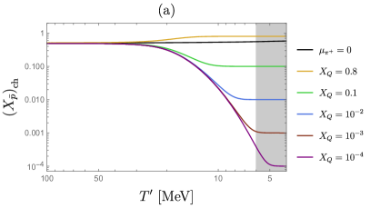
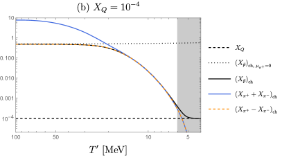
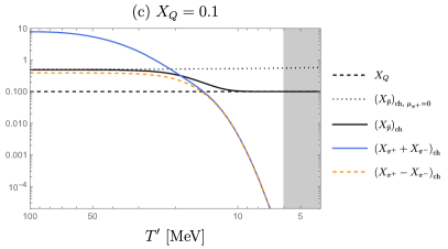
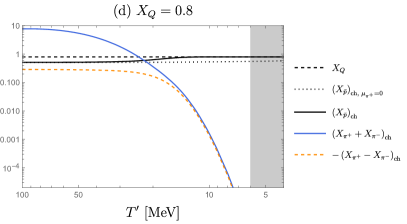
Figure 8: Chemical-equilibrium abundances for different charged-pion chemical-potential $\mu_{\pi^{+}}$ assumptions. The benchmark parameters $T_{0}=100\mathinner{\mathrm{MeV}}$, $\bar{\eta}=10^{-2}$, $R_{0}=1.5\text{ mm}$ are assumed in these plots. Panel (a): The chemical-equilibrium abundance of anti-protons $\left(X_{\bar{p}}\right)_{\rm ch}$ as a function of the comoving temperature $T^{\prime}$ for different values of $X_{Q}$ [defined at Eq. (70)]; the $\left(X_{\bar{p}}\right)_{\rm ch}$ for $\mu_{\pi^{+}}=0$ is also shown for comparison. Panels (b)–(d): The chemical-equilibrium abundances of anti-protons $\left(X_{\bar{p}}\right)_{\rm ch}$, symmetric population of charged pions $\left(X_{\pi^{+}}+X_{\pi^{-}}\right)_{\rm ch}$, and anti-symmetric population of charged pions $\pm\left(X_{\pi^{+}}-X_{\pi^{-}}\right)_{\rm ch}$ as a function of the comoving temperature $T^{\prime}$ for the selected parameter values $X_{Q}=10^{-4}$, $X_{Q}=0.1$, and $X_{Q}=0.8$, respectively. For comparison, we also show $X_{Q}$ and $\left(X_{\bar{p}}\right)_{\rm ch}$ for $\mu_{\pi^{+}}=0$ (as assumed in Sec. III.3.3). The gray-shaded regions are where we expect $X_{\bar{p}}$ and $X_{\pi^{\pm}}$ to be given by their freeze-out values, instead of the chemical-equilibrium values, $\left(X_{\bar{p}}\right)_{\rm ch}$ and $\left(X_{\pi^{\pm}}\right)_{\rm ch}$, that are shown in (or inferable from) these plots.

Knowing $\mu_{\pi^{+}}(X_{Q},T^{\prime})$ allows us to compute the chemical-equilibrium abundances of anti-protons and charged pions; see Fig. 8. At high temperatures, chemical potentials are insignificant and consequently particles are thermally populated in a democratic way, yielding $\left(X_{\bar{p}}\right)_{\rm ch}\approx\left(X_{\bar{n}}\right)_{\rm ch}\approx 0.5$ and (to keep charge neutrality) $\left(X_{\pi^{+}}-X_{\pi^{-}}\right)_{\rm ch}\approx 0.5$. On the other hand, at low temperatures, thermodynamics favors storing charge asymmetry in $\bar{p}$ rather than $\pi^{\pm}$. Very approximately, this can be understood heuristically in the following way. We have assumed a net anti-baryon number for the plasma. Because baryon number is conserved in the plasma, a fixed number of anti-nucleons (forming the net anti-baryon asymmetry) therefore automatically exist in the plasma at any temperature, either as $\bar{n}$ or $\bar{p}$; specifically, the mass of these particles need not be extracted from the thermal bath in order for them to be in existence. We have also assumed a non-zero negative charge asymmetry on the hadronic sector, and charge is also conserved in the plasma. An anti-proton $\bar{p}$ kills two birds with one proverbial stone: it can carry both baryon number and charge. By contrast, pions do not carry baryon number and therefore are not automatically in existence in the plasma in any abundance: they must be created thermally; i.e., their rest-mass energy must be extracted from the thermal bath. Effectively, it therefore costs much more energy to create a massive $\pi^{-}$ thermally from the bath in order to store negative charge on it, than it does to simply store the charge on $\bar{p}$. As a result, unless $X_{Q}\lesssim 10^{-4}$, most of the charge asymmetry $X_{Q}$ typically ends up in anti-protons, such that $X_{\bar{p}}\approx X_{Q}$ well before the SMCER interactions decouple.

Figure 9: The abundances of nuclear species $X_{i}=n^{\prime}_{i}/n^{\prime}_{\bar{B}}$ (solid and dashed colored lines, as identified in the legend) as a function of the comoving fireball temperature $T^{\prime}$, computed by numerically solving the Boltzmann equations for a simplified nuclear-reaction network detailed in Appendix C, for a fireball with $T_{0}=100\,\mathinner{\mathrm{MeV}}$, $R_{0}=1.5\,\text{cm}$, $\bar{\eta}=10^{-2}$ ($\Gamma=10$). Note that this plot is similar to Fig. 2; however, instead of neglecting the charged pion chemical potential, here we set $X_{Q}=10^{-2}$ such that $\mu_{\pi^{+}}=28.8\mathinner{\mathrm{MeV}}$, $X_{\bar{p}}=0.01$, and $X_{\bar{n}}=0.99$, all evaluated at $T^{\prime}\approx 6\mathinner{\mathrm{MeV}}$. Note that $R_{0}$ here is an order of magnitude larger than in Fig. 2.

Starting at a sufficiently high $T_{0}$ ($\gtrsim 10\mathinner{\mathrm{MeV}}$), the actual comoving number densities of $\bar{n}$, $\bar{p}$, and $\pi^{\pm}$ closely track their chemical-equilibrium values (obtained from equilibrium thermodynamics as we have computed above) until they eventually freeze out once $\pi^{\pm}$ become too Boltzmann suppressed to keep the SMCER interactions efficient. We found that the decoupling temperature $T^{\prime}_{\bar{n}\bar{p}}$ varies slightly in the range $6\mathinner{\mathrm{MeV}}\lesssim T^{\prime}_{\bar{n}\bar{p}}\lesssim 8\mathinner{\mathrm{MeV}}$ when $X_{Q}$ is varied in the range $0\leq X_{Q}\leq 1$. Importantly, for $X_{Q}\gtrsim 10^{-3}$, we find that $X_{\bar{p}}(T^{\prime})\rightarrow X_{Q}$ already for $T^{\prime}>T^{\prime}_{\bar{n}\bar{p}}$; see Fig. 8. This means that we can indeed rely on our equilibrium thermodynamics arguments above to establish that the charge asymmetry $X_{Q}$ is maintained on the anti-protons in this regime.

In general, we find that having $X_{Q}\sim 1-X_{Q}\sim\mathcal{O}(1)$ results in $X_{\bar{n}}/X_{\bar{p}}\sim\mathcal{O}(1)$ at SMCER decoupling; see Fig. 8. Because there are only $\mathcal{O}(1)$ quantitative changes to the anti-nucleosynthetic abundance results in the main text for more general values for $X_{\bar{n}}/X_{\bar{p}}\sim\mathcal{O}(1)$ than the value of $X_{\bar{n}}/X_{\bar{p}}\approx 0.8$ that we used in Sec. III.3.3 (under the more restrictive assumption of $\mu_{\pi^{+}}=0$), this implies that the same qualitative conclusions that we reached in the main text will continue to hold for any values of $X_{Q}\sim 1-X_{Q}\sim\mathcal{O}(1)$. This is turn is significant because, in order to achieve $\mu_{\pi^{+}}=0$ exactly at $T^{\prime}_{\bar{n}\bar{p}}$ (as we assumed in Sec. III.3.3) we would need to choose $X_{Q}$ such that it almost exactly matches the freeze-out anti-proton abundance in the absence of $\mu_{\pi^{+}}$: i.e., $X_{Q}\approx\left(X_{\bar{p}}\right)_{\text{ch}}|_{\mu_{\pi^{+}}=0}\approx 0.56$. Were that exact value a crucial input to the anti-nucleosynthesis analysis, this would constitute a fine tuning because $X_{Q}$ is supposed to be set by pre-thermalization physics which has no connection to the post-thermalization physics (although see the discussion in the last paragraph of this Appendix below). Our analysis in this Appendix thus establishes that our main-text analysis is not finely tuned.

Next, we discuss how the fireball outputs are affected if $\mu_{\pi^{+}}\gg m_{n}-m_{p}$. In this case, we generically have $X_{\bar{p}}\ll 1$ at SMCER decoupling. However, even then, a $X_{{}^{4}\overline{\text{He}}}/X_{{}^{3}\overline{\text{He}}}\sim 1/2$ anti-helium isotope ratio can still be obtained without overproducing anti-protons; i.e., $X_{\bar{n}}+X_{\bar{p}}\lesssim 10^{5}X_{{}^{4}\overline{\text{He}}}$ when the fireball becomes optically thin, in order to avoid violating the $1\sigma$ uncertainties on the AMS-02 anti-proton flux [72]; see Fig. 6. To demonstrate this, we show in Fig. 9 the evolution of nuclear abundances in this $\mu_{\pi^{+}}\gg m_{n}-m_{p}$ case with $X_{Q}=10^{-2}$ and other parameters chosen to explain the AMS-02 candidate anti-helium events. The freeze-out abundances shown in Fig. 9 are marginally consistent with the anti-proton flux observed at AMS-02. To explain the anti-helium isotope ratio with $X_{Q}\lesssim 10^{-2}$ would however lead to an overproduction of anti-protons. Therefore, compatibility with the AMS-02 data requires $X_{Q}\gtrsim 10^{-2}$. Note, however, that the marginal set parameters we picked for Fig. 9 to complement $X_{Q}=10^{-2}$ could be interesting from the perspective of the $\sim 10\%$ anti-proton excess [65].

We have so far treated the charge asymmetry $X_{Q}$ as a free parameter. In actuality, it depends both on the properties of the initial particle injection, which are model-dependent but could naturally give $X_{Q}\sim 1$, and post-injection SM processes. In case the initial injection does not produce a considerable charge asymmetry, some degree of $X_{Q}$ can arise spontaneously from non-equilibrium Standard Model processes occurring before or after thermalization. Electroweak process such as $\bar{n}+e^{-}\leftrightarrow\bar{p}+\nu_{e}$ and its variants can transfer charges between the hadron and lepton sectors; however, they have a preferred charge-transfer direction only at sufficiently low temperatures, $T^{\prime}\lesssim m_{n}-m_{p}$, at which point electroweak interaction rates are extremely suppressed (given the dynamical timescales involved in the fireball expansion). A higher contribution to $X_{Q}$ arises from the decay of (a small fraction of) charged pions. As shown in Fig. 8(b), even if we start with $X_{Q}$ being virtually zero, a charge asymmetry of $X_{\pi^{+}}-X_{\pi^{-}}\approx 0.5$ is automatically present in $\pi^{\pm}$ at high temperatures (SMCER reactions are efficient, so if $X_{Q}\ll 1$, we have $X_{\bar{p}}\sim X_{\pi^{+}}-X_{\pi^{-}}$). Within the initial fireball expansion timescale (during which the bulk plasma motion is non-relativistic), a fraction $10^{-4}\lesssim R_{0}/\tau_{\pi^{\pm}}\lesssim 10^{-1}$ (for $1\,\text{mm}\lesssim R_{0}\lesssim 1\,\text{m}$) of the charged pions decay to charged muons [$\pi^{\pm}\rightarrow\mu^{\pm}+\nu_{\mu}(\bar{\nu}_{\mu})$ with $\tau_{\pi^{\pm}}\sim 2.6\times 10^{-8}\,\text{s}$ [73]], thereby generating $X_{Q}\sim(X_{\pi^{+}}-X_{\pi^{-}})(R_{0}/\tau_{\pi^{\pm}})$ in the range $5\times 10^{-5}\lesssim X_{Q}\lesssim 5\times 10^{-2}$. Unfortunately, at least for the benchmark $\sim 1\,\text{mm}$ parameters we used in the main text (or the benchmark $R_{0}\sim 1\,\text{cm}$ used in Fig. 9), this spontaneously generated $X_{Q}$ is too small to be phenomenologically viable in light of the AMS anti-proton results (see discussion above).

Appendix C Simplified nuclear reaction network

Anti-neutrons and anti-protons in the fireball plasma are initially held in chemical equilibrium by charged-pion–mediated anti-neutron–anti-proton interconversions (i.e., SMCER) at $10\lesssim T^{\prime}\lesssim 200\,\mathinner{\mathrm{MeV}}$. As found in Sec. III.3.3, such interconversion process decouples relatively early, at $T_{\bar{n}\bar{p}}^{\prime}\approx 6\,\mathinner{\mathrm{MeV}}$, when there are virtually no nuclear bound states present. On the other hand, photodissociation stalls the synthesis of anti-deuterium (and the whole nuclear chain) until the temperature is considerably below the anti-deuterium binding energy $B_{D}\approx 2.2\,\mathinner{\mathrm{MeV}}$, at $T_{\rm D}^{\prime}\sim 140-170\,\mathinner{\mathrm{keV}}$, by which point the anti-neutron–to–anti-proton ratio has completely frozen out. Hence, we can treat the anti-neutron–anti-proton decoupling separately from the whole nuclear reaction chain. In our numerical procedure, we thus first solve for the freeze-out ratio of $n^{\prime}_{\bar{n}}/n^{\prime}_{\bar{p}}$ ignoring nuclear reactions, finding $n^{\prime}_{\bar{n}}/n^{\prime}_{\bar{p}}\approx 0.8$ per Eq. (19) [assuming $\mu_{\pi^{+}}=0$; similar results could be derived for more general $X_{Q}$ as discussed in Appendix B], and use this as an input when solving the Boltzmann equations governing the subsequent nuclear reactions.

We now describe our simplified nuclear reaction network governing the evolution of relative abundances of elements, $X_{i}=n^{\prime}_{i}/n^{\prime}_{\bar{B}}$. We consider only elements with $A\leq 4$, namely $\bar{p}$, $\bar{n}$, ${\mkern-2.0mu\bar{\mkern 2.0mu\text{D}}}$, ${\bar{\text{T}}}$, ${}^{3}\overline{\text{He}}$, and ${}^{4}\overline{\text{He}}$. Heavier species with $A>4$ such as $\overline{\text{Li}}$ and $\overline{\text{Be}}$ isotopes are virtually absent and have negligible impacts on the $A\leq 4$ elements that we consider. Conservation of baryon number ensures $\sum_{i}A_{i}X_{i}=1$, with $A_{i}$ being the atomic mass number of the nuclear species $i$. This can be used to solve for the abundance of one element, which we take to be $X_{\bar{p}}$, given the other abundances

$$X_{\bar{p}}=1-\sum_{i\neq\bar{p}}A_{i}X_{i}\>.$$ (78)

We set as the initial conditions

$$X_{\bar{p}} =0.56\>, X_{\bar{n}} =0.44\>, X_{i\notin\{\bar{n},\bar{p}\}} =0\>,$$ (79)

per Eq. (19) at an initial temperature $T^{\prime}=1\,\mathinner{\mathrm{MeV}}$, and evolve the abundances of elements other than $\bar{p}$ with the following simplified nuclear reaction network [122]:

$$-\frac{dX_{\bar{n}}}{d\ln T^{\prime}} \approx\frac{\epsilon_{\rm nuc}(T^{\prime})}{\text{mb}}\left(\begin{array}[]{l}-\left<\sigma v\right>_{\bar{p}\bar{n}}X_{\bar{p}}X_{\bar{n}}+\left<\sigma v\right>_{{\mkern-2.0mu\bar{\mkern 2.0mu\text{D}}}\gamma}X_{{\mkern-2.0mu\bar{\mkern 2.0mu\text{D}}}}Y_{{\mkern-2.0mu\bar{\mkern 2.0mu\text{D}}}\gamma}+\left<\sigma v\right>_{{\mkern-2.0mu\bar{\mkern 2.0mu\text{D}}}{\mkern-2.0mu\bar{\mkern 2.0mu\text{D}}}}X_{{\mkern-2.0mu\bar{\mkern 2.0mu\text{D}}}}^{2}+\left<\sigma v\right>_{{\bar{\text{T}}}{\mkern-2.0mu\bar{\mkern 2.0mu\text{D}}}}X_{{\bar{\text{T}}}}X_{{\mkern-2.0mu\bar{\mkern 2.0mu\text{D}}}}-\left<\sigma v\right>_{{\mkern-2.0mu\bar{\mkern 2.0mu\text{D}}}\bar{n}}X_{{\mkern-2.0mu\bar{\mkern 2.0mu\text{D}}}}X_{\bar{n}}\\[8.61108pt] -\left<\sigma v\right>_{{}^{3}\overline{\text{He}}\bar{n}}X_{{}^{3}\overline{\text{He}}}X_{\bar{n}}+\left<\sigma v\right>_{{}^{3}\overline{\text{He}}\gamma}X_{{}^{3}\overline{\text{He}}}Y_{{}^{3}\overline{\text{He}}\gamma}\end{array}\right)\>;$$ (82)

$$-\frac{dX_{{\mkern-2.0mu\bar{\mkern 2.0mu\text{D}}}}}{d\ln T^{\prime}} \approx\frac{\epsilon_{\rm nuc}(T^{\prime})}{\text{mb}}\left(\begin{array}[]{l}\left<\sigma v\right>_{\bar{p}\bar{n}}X_{\bar{p}}X_{\bar{n}}-\left<\sigma v\right>_{{\mkern-2.0mu\bar{\mkern 2.0mu\text{D}}}\gamma}X_{{\mkern-2.0mu\bar{\mkern 2.0mu\text{D}}}}Y_{{\mkern-2.0mu\bar{\mkern 2.0mu\text{D}}}\gamma}-\left<\sigma v\right>_{{\mkern-2.0mu\bar{\mkern 2.0mu\text{D}}}{\mkern-2.0mu\bar{\mkern 2.0mu\text{D}}}}X_{{\mkern-2.0mu\bar{\mkern 2.0mu\text{D}}}}^{2}-\left<\sigma v\right>_{{\mkern-2.0mu\bar{\mkern 2.0mu\text{D}}}\bar{p}}X_{{\mkern-2.0mu\bar{\mkern 2.0mu\text{D}}}}X_{\bar{p}}-\left<\sigma v\right>_{{\mkern-2.0mu\bar{\mkern 2.0mu\text{D}}}\bar{n}}X_{{\mkern-2.0mu\bar{\mkern 2.0mu\text{D}}}}X_{\bar{n}}\\[8.61108pt] -\left<\sigma v\right>_{{\bar{\text{T}}}{\mkern-2.0mu\bar{\mkern 2.0mu\text{D}}}}X_{{\bar{\text{T}}}}X_{{\mkern-2.0mu\bar{\mkern 2.0mu\text{D}}}}-\left<\sigma v\right>_{{}^{3}\overline{\text{He}}{\mkern-2.0mu\bar{\mkern 2.0mu\text{D}}}}X_{{}^{3}\overline{\text{He}}}X_{{\mkern-2.0mu\bar{\mkern 2.0mu\text{D}}}}\end{array}\right)\>;$$ (85)

$$-\frac{dX_{{\bar{\text{T}}}}}{d\ln T^{\prime}} \approx\frac{\epsilon_{\rm nuc}(T^{\prime})}{\text{mb}}\Big{(}\left<\sigma v\right>_{{\mkern-2.0mu\bar{\mkern 2.0mu\text{D}}}{\mkern-2.0mu\bar{\mkern 2.0mu\text{D}}}}X_{{\mkern-2.0mu\bar{\mkern 2.0mu\text{D}}}}^{2}+\left<\sigma v\right>_{{\mkern-2.0mu\bar{\mkern 2.0mu\text{D}}}\bar{n}}X_{{\mkern-2.0mu\bar{\mkern 2.0mu\text{D}}}}X_{\bar{n}}+\left<\sigma v\right>_{{}^{3}\overline{\text{He}}\bar{n}}X_{{}^{3}\overline{\text{He}}}X_{\bar{n}}-\left<\sigma v\right>_{{\bar{\text{T}}}{\mkern-2.0mu\bar{\mkern 2.0mu\text{D}}}}X_{{\bar{\text{T}}}}X_{{\mkern-2.0mu\bar{\mkern 2.0mu\text{D}}}}\Big{)}\>;$$ (86)

$$-\frac{dX_{{}^{3}\overline{\text{He}}}}{d\ln T^{\prime}} \approx\frac{\epsilon_{\rm nuc}(T^{\prime})}{\text{mb}}\left(\begin{array}[]{l}\left<\sigma v\right>_{{\mkern-2.0mu\bar{\mkern 2.0mu\text{D}}}{\mkern-2.0mu\bar{\mkern 2.0mu\text{D}}}}X_{{\mkern-2.0mu\bar{\mkern 2.0mu\text{D}}}}^{2}+\left<\sigma v\right>_{{\mkern-2.0mu\bar{\mkern 2.0mu\text{D}}}\bar{p}}X_{{\mkern-2.0mu\bar{\mkern 2.0mu\text{D}}}}X_{\bar{p}}-\left<\sigma v\right>_{{}^{3}\overline{\text{He}}\gamma}X_{{}^{3}\overline{\text{He}}}Y_{{}^{3}\overline{\text{He}}\gamma}-\left<\sigma v\right>_{{}^{3}\overline{\text{He}}\bar{n}}X_{{}^{3}\overline{\text{He}}}X_{\bar{n}}\\[8.61108pt] -\left<\sigma v\right>_{{}^{3}\overline{\text{He}}{\mkern-2.0mu\bar{\mkern 2.0mu\text{D}}}}X_{{}^{3}\overline{\text{He}}}X_{{\mkern-2.0mu\bar{\mkern 2.0mu\text{D}}}}\end{array}\right)\>;$$ (89)

$$-\frac{dX_{{}^{4}\overline{\text{He}}}}{d\ln T^{\prime}} \approx\frac{\epsilon_{\rm nuc}(T^{\prime})}{\text{mb}}\Big{(}\left<\sigma v\right>_{{\bar{\text{T}}}{\mkern-2.0mu\bar{\mkern 2.0mu\text{D}}}}X_{{\bar{\text{T}}}}X_{{\mkern-2.0mu\bar{\mkern 2.0mu\text{D}}}}+\left<\sigma v\right>_{{}^{3}\overline{\text{He}}{\mkern-2.0mu\bar{\mkern 2.0mu\text{D}}}}X_{{}^{3}\overline{\text{He}}}X_{{\mkern-2.0mu\bar{\mkern 2.0mu\text{D}}}}\Big{)}\>,$$ (90)

where we have defined the dimensionless quantity

$$\epsilon_{\rm nuc}(T^{\prime})=\bar{\eta}n_{\gamma}^{\prime}\times\text{mb}\times\tau^{\prime}(T^{\prime})\>,$$ (91)

which quantifies the efficiency of nuclear reactions in the timescale of fireball expansion. Apart from anti-deuterium photodissociation, we include in the above set of equations only thresholdless (forward) reactions. The reverse processes to these reactions are endothermic, and are suppressed by factors of the form $e^{-Q/T^{\prime}}$ (where $Q$ is the threshold energy of the reverse reaction; i.e., the energy liberated in the forward reaction) in their thermally averaged cross section as well as the smallness (verified a posteriori) of the $X_{i}$ factors relative to those of the forward reactions. It is nevertheless important to take into account anti-deuterium photodissociation due to its uniquely low threshold energy and the potentially large photon abundance. The abundance of photons energetic enough to photodissociate the nuclear species $i$ is

$$Y_{i\gamma}=\frac{n^{\prime}_{\gamma}(E^{\prime}_{\gamma}>Q_{i})}{n^{\prime}_{\bar{B}}}\sim\frac{Q_{i}^{2}}{\bar{\eta}T^{\prime 2}}e^{-Q_{i}/T^{\prime}}\>.$$ (92)

where $Q_{i}$ is the threshold energy of that process. The photodissociation cross-sections as functions of energy typically rise sharply at $E_{\gamma}\approx Q_{i}$ and fall of smoothly at higher $E_{\gamma}$. We approximate the thermal averaged photodissociation cross-sections $\left<\sigma v\right>_{i\gamma}$ with their near-threshold values. We consider only the photodissociation processes ${\mkern-2.0mu\bar{\mkern 2.0mu\text{D}}}+\gamma\rightarrow\bar{p}+\bar{n}$, with $Q_{{\mkern-2.0mu\bar{\mkern 2.0mu\text{D}}}}=2.2\,\mathinner{\mathrm{MeV}}$ and $\left<\sigma v\right>_{{\mkern-2.0mu\bar{\mkern 2.0mu\text{D}}}\gamma}\approx 2.5\,\text{mb}$ [123]. The other ones have significantly higher threshold energies $Q_{i}$ and are consequently much less efficient due to the exponentially suppressed $E_{\gamma}\gtrsim Q_{i}$ photon abundance (as considered at the temperature $T^{\prime}\sim 100\,\mathinner{\mathrm{keV}}$ when anti-nucleosynthesis is efficient).

Appendix D Nuclear cross sections

Figure 10: The assumed values of thermal-average cross sections for (anti-)nuclear reactions as a function of temperature $T^{\prime}$.

We assume that the nuclear cross-sections for purely anti-matter processes are equal to those of the analogous reactions involving matter. For completeness, we list here the thermal averaged nuclear cross sections from [41, 43, 124, 125] and express them in terms of the temperature ratio $T_{9}\equiv T^{\prime}/(10^{9}\,\text{K})=T^{\prime}/(86\,\mathinner{\mathrm{keV}})$:

• $\bar{n}+\bar{p}\rightarrow{\mkern-2.0mu\bar{\mkern 2.0mu\text{D}}}+\gamma$ ($Q=2.22\,\mathinner{\mathrm{MeV}}$)

  $$\left.\left<\sigma v\right>_{\bar{n}\bar{p}}\right|_{T^{\prime}\sim 100\,\mathinner{\mathrm{keV}}} \approx 2\times 10^{-3}\,\text{mb}\>.$$

• ${\mkern-2.0mu\bar{\mkern 2.0mu\text{D}}}+{\mkern-2.0mu\bar{\mkern 2.0mu\text{D}}}\rightarrow{}^{3}\overline{\text{He}}+\bar{n}$ ($Q=3.26\,\mathinner{\mathrm{MeV}}$) and ${\mkern-2.0mu\bar{\mkern 2.0mu\text{D}}}+{\mkern-2.0mu\bar{\mkern 2.0mu\text{D}}}\rightarrow{\bar{\text{T}}}+\bar{p}$ ($Q=4.03\,\mathinner{\mathrm{MeV}}$). For each,

  $$\left<\sigma v\right>_{\rm{\mkern-2.0mu\bar{\mkern 2.0mu\text{D}}}{\mkern-2.0mu\bar{\mkern 2.0mu\text{D}}}}\approx 100\,\text{mb}\times T_{9}^{-2/3}e^{-4.3T_{9}^{-1/3}}\>.$$

• ${\mkern-2.0mu\bar{\mkern 2.0mu\text{D}}}+\bar{p}\rightarrow{}^{3}\overline{\text{He}}+\gamma$ ($Q=5.49\,\mathinner{\mathrm{MeV}}$)

  $$\left<\sigma v\right>_{{\mkern-2.0mu\bar{\mkern 2.0mu\text{D}}}\bar{p}}\approx 3\times 10^{-4}\,\text{mb}\times T_{9}^{-2/3}e^{-3.7T_{9}^{-1/3}}\>.$$

• ${\mkern-2.0mu\bar{\mkern 2.0mu\text{D}}}+\bar{n}\rightarrow{\bar{\text{T}}}+\gamma$ ($Q=6.24\,\mathinner{\mathrm{MeV}}$)

  $$\left.\left<\sigma v\right>_{{\mkern-2.0mu\bar{\mkern 2.0mu\text{D}}}\bar{n}}\right|_{T^{\prime}\sim 100\,\mathinner{\mathrm{keV}}}\approx 1\times 10^{-4}\,\text{mb}\>.$$

• ${\bar{\text{T}}}+{\mkern-2.0mu\bar{\mkern 2.0mu\text{D}}}\rightarrow{}^{4}\overline{\text{He}}+\bar{n}$ ($Q=17.59\,\mathinner{\mathrm{MeV}}$)

  $$\left<\sigma v\right>_{{\bar{\text{T}}}{\mkern-2.0mu\bar{\mkern 2.0mu\text{D}}}}\approx 30\,\text{mb}\times T_{9}^{-2/3}e^{-0.5T_{9}^{-1}}\>.$$

• ${}^{3}\overline{\text{He}}+{\mkern-2.0mu\bar{\mkern 2.0mu\text{D}}}\rightarrow{}^{4}\overline{\text{He}}+\bar{p}$ ($Q=18.35\,\mathinner{\mathrm{MeV}}$)

  $$\left<\sigma v\right>_{{}^{3}\overline{\text{He}}{\mkern-2.0mu\bar{\mkern 2.0mu\text{D}}}}\approx 30\,\text{mb}\times T_{9}^{-1/2}e^{-1.8T_{9}^{-1}}\>.$$

• ${}^{3}\overline{\text{He}}+\bar{n}\rightarrow{\bar{\text{T}}}+\bar{p}$ ($Q=0.76\,\mathinner{\mathrm{MeV}}$)

  $$\left.\left<\sigma v\right>_{{}^{3}\overline{\text{He}}\bar{n}}\right|_{T^{\prime}\sim 100\,\mathinner{\mathrm{keV}}}\approx 40\,\text{mb}\>.$$

We show these cross sections in Fig. 10, rescaled as appropriate to fit them all on the same plot. Most important to our analysis are cross-sections at temperatures $T^{\prime}\sim 100$–$200\,\mathinner{\mathrm{keV}}$ where anti-nucleosynthesis mainly occurs. We neglect the mild temperature dependences of the cross-sections for processes that do not suffer from Coulomb-barrier suppression.

Appendix E Changes in the number of degrees of freedom

Here we account for the effect of changes in the number of degrees of freedom $g_{*}$ on the fireball expansion dynamics (see Sec. III.2), neglecting the small differences between the $g_{*}$ for entropy and energy density [126]; i.e., we assume $g_{*S}=g_{*\rho}=g_{*}$. We first write the energy and entropy conservation equations, respectively, for each of the shells (assumed relativistic, with $v\sim 1$) in more general forms:

$$\gamma^{2}(\rho^{\prime}+p^{\prime})r^{2}\delta r \approx\text{constant}\>,$$ (93)

$$\gamma s^{\prime}r^{2}\delta r \approx\text{constant}\>.$$ (94)

In cases of our interest, the fireball can be approximated as consisting of only radiation (photons and relativistic massive species) and (anti-)matter (dominated by anti-baryons), allowing us to write

$$\rho^{\prime}+p^{\prime}\approx\begin{cases}s^{\prime}T^{\prime},&T^{\prime}\gg\bar{\eta}m_{p}\\ \bar{\eta}s^{\prime}m_{p},&T^{\prime}\ll\bar{\eta}m_{p}\end{cases}\>,$$ (95)

where $s^{\prime}T^{\prime}$ and $\bar{\eta}s^{\prime}m_{p}$ are the contributions from radiation and (anti-)matter, respectively, and we used $\bar{\eta}\equiv n_{\bar{B}}/s^{\prime}$. Eliminating $r$ from the energy and entropy conservation equations, and using $\Gamma\equiv T_{0}/(\bar{\eta}m_{p})$, we find

$$\gamma\left(T^{\prime}+\frac{T_{0}}{\Gamma}\right)\sim\text{constant}\>.$$ (96)

Substituting $s^{\prime}\propto g_{*}(T^{\prime})\times(T^{\prime})^{3}$, Eq. (96), and Eq. (67) into Eq. (94), we obtain an equation that determines the evolution of $T^{\prime}$ with $r$:

$$g_{*}(T^{\prime})\left(\frac{T^{{}^{\prime}3}}{T^{\prime}+T_{0}/\Gamma}\right)r^{2}$$

$$\qquad\times\left[R_{0}+\left(\frac{T^{\prime}+T_{0}/\Gamma}{T_{0}}\right)^{2}r\right]\sim\text{constant}\>,$$ (97)

which shows how the temperature-radius relation $T^{\prime}(r)$ is modified in the presence of changes in $g_{*}(T^{\prime})$ compared to the $T_{g_{*}=2}^{\prime}(r)$ for constant $g_{*}=2$ assumed in the main text. During RD ($T^{\prime}\gtrsim T_{0}/\Gamma$), we thus have

$$T^{\prime} \sim\left[\frac{g_{*}(T^{\prime})}{g_{*}(T_{0})}\right]^{-1/2}T_{g_{*}=2}^{\prime} \text{[RD]}\>;$$ (99)

$$\rho^{\prime} \sim g_{*}(T^{\prime})\times T^{\prime 4}\propto\left[\frac{g_{*}(T^{\prime})}{g_{*}(T_{0})}\right]^{-1}\rho_{g_{*}=2}^{\prime} \text{[RD]}\>,$$ (100)

while during MD ($T^{\prime}\gtrsim T_{0}/\Gamma$) we have

$$T^{\prime} \propto\left[\frac{g_{*}(T^{\prime})}{g_{*}(T_{0}/\Gamma)}\right]^{-1/3}T_{g_{*}=2}^{\prime} \text{[MD]}\>;$$ (101)

$$\rho^{\prime} \propto g_{*}(T^{\prime})\times T^{\prime 3}\propto[g_{*}(T^{\prime})]^{0} \text{[MD]}\>.$$ (102)

Notice that the impact of a change in $g_{*}$ is weak if it occurs during matter domination.

In our scenario, the effective number of relativistic degrees of freedom of the fireball $g_{*}$ is given by

$$g_{*}(T^{\prime})=\begin{cases}12\ ,&100\,\mathinner{\mathrm{MeV}}\lesssim T^{\prime}\lesssim 200\,\mathinner{\mathrm{MeV}}\>;\\ 5.5\ ,&\phantom{00}1\,\mathinner{\mathrm{MeV}}\lesssim T^{\prime}\lesssim 100\,\mathinner{\mathrm{MeV}}\>;\\ 2\ ,&\phantom{\,100\,\mathinner{\mathrm{MeV}}\lesssim}T^{\prime}\lesssim 1\,\mathinner{\mathrm{MeV}}\>;\end{cases}$$ (103)

reflecting, respectively, the contributions from the sets of particles $\{\pi^{0,\pm},e^{\pm},\mu^{\pm},\gamma\}$, $\{e^{\pm},\gamma\}$, and $\{\gamma\}$ in each temperature range. That is, we have two possible “jumps” in $g_{*}$, happening at $T^{\prime}\sim 100\,\mathinner{\mathrm{MeV}}$ and $T^{\prime}\sim 1\,\mathinner{\mathrm{MeV}}$ (the transitions of course are smooth, but abrupt). Since we require $10\,\mathinner{\mathrm{MeV}}\lesssim T_{0}\lesssim 100\,\mathinner{\mathrm{MeV}}$ and $\Gamma\sim 10$, only the jump at $T^{\prime}\sim 100\,\mathinner{\mathrm{MeV}}$ has a chance to spoil the accuracy of the constant-$g_{*}$ approximation adopted in the main analysis. This jump at $T^{\prime}\sim 100\,\mathinner{\mathrm{MeV}}$ amounts to an error in the analytical estimate for $T^{\prime}(r)$ by a factor of $\sqrt{12/5.5}\approx 1.5$ and that for $\rho^{\prime}(r)$ by a factor of $12/5.5\approx 2.2$. These are within the level precision we are aiming for, given that our analysis does not fully capture the effects of the inhomogeneity and initial evolution of the fireball, which would also introduce $\mathcal{O}(1)$ uncertainties in our estimates for $T^{\prime}(r)$. Note that the Lorentz factor $\gamma$ remains to be related to the temperature $T^{\prime}$ as given in Eq. (96).

Although $T^{\prime}$ appears at various places in the Boltzmann Eqs. (82)–(90) [it plays the role of time, appears in the cross sections, and controls $Y_{i\gamma}$], its relation to the shell radius $r$, namely $T^{\prime}(r)$ [which is affected by changes in $g_{*}(T^{\prime})$], only enters via $\epsilon_{\rm nuc}(T^{\prime})$, as defined in Eq. (91), through the comoving expansion timescale $\tau^{\prime}(T^{\prime})$. The latter is given by Eq. (10) in the absence of changes in $g_{*}(T^{\prime})$ and would change by a mild $\mathcal{O}(1)$ factor when the effects of changes in $g_{*}(T^{\prime})$ are included. This amounts to a slight shift in the value of $T_{0}$ in relation to $R_{0}$ that yields a given $\tau^{\prime}$. Since $\tau^{\prime}$ controls the output nuclear abundances, the lines of constant anti-helium isotope ratio in, e.g., Fig. 4, would be displaced, though only slightly.

Appendix F Prompt (‘burst’) or slow (‘wind’) injection

The duration of the anti-quark injection $t_{*}$ can be shorter $t_{*}\lesssim R_{*}$ (burst regime) or longer $t_{*}\gtrsim R_{*}$ (wind regime) than the spatial size of the injection $R_{*}$.

Following the injection, the anti-quarks will have the following number density profile if they do not interact with one another and simply free stream away

$$n_{B,0}(r) \sim\zeta_{*}\times\frac{E_{*}}{m_{\textsc{dm}}R_{*}^{3}}\times\text{min}\left(1,\frac{R_{*}^{2}}{r^{2}}\right)\>,$$ (104)

where $r$ the radius from the center of a spherical the injection region of radius $R_{*}$, $E_{*}$ is the total energy of the injected SM particles, and the factor

$$\zeta_{*}\sim\text{min}\left(1,\frac{R_{\rm*}}{t_{\rm*}}\right)\lesssim 1$$ (105)

accounts for the burst vs. wind branching of cases: in the wind case the density of the injected anti-quarks within $R_{*}$ is diluted by a factor of $R_{*}/t_{*}$.

Regardless of the relative sizes of $t_{*}$ and $R_{*}$, the probability that an anti-quark undergoes a process of any sort before arriving at a radius $r$, $P(r)\sim n_{B,0}(r)\sigma v_{\rm rel}\times r\propto r^{-1}$, decreases with $r$ for $r\gg R_{*}$, where we have assumed that the relative velocity is relativistic $v_{\rm rel}\sim 1$ and the cross section $\sigma$ is independent of $r$. It follows that in order for these particles to thermalize, the thermalization rate needs to be efficient inside the injection region; i.e., $\Gamma_{\rm th}\gtrsim R_{*}^{-1}$ at $r\lesssim R_{*}$.

Once the fireball can achieve thermalization and has attained a semirelativistic bulk radial velocity $v\sim 1$, its subsequent evolution is completely described by the fireball temperature $T_{0}$ and radius $R_{0}$ when it first thermalizes (as well as $X_{Q}$), and these are given by

$$T_{0} \sim\left(\frac{\zeta_{*}E_{*}}{R_{*}^{3}}\right)^{1/4}\>,$$ (106)

$$R_{0} \sim R_{*}\>.$$ (107)

Note that the anti-baryon–to–entropy ratio $\bar{\eta}$ does not depend on the relative size between $t_{*}$ and $R_{*}$.

As explained in Appendix A, the plasma outflow can be treated as a series independent differential radial slices which separately go through nearly the same thermal and hydrodynamical evolution. In each of these slices, anti-nucleosynthesis proceeds as described in Sec. III. The only difference is that $T_{0}$ and $R_{0}$ are now more generally given by Eqs. (106) and (107). Since the abundances of nuclear species $\left.X_{i}\right|_{\rm inj.}$ released by each radial slice are completely determined by the set of parameters $(T_{0},R_{0},\bar{\eta},X_{Q})$ which are essentially the same for all the shells, the numbers of anti-nuclei or anti-nucleons $N_{i}|_{\rm inj.}$ released into the ISM are still given by $N_{i}|_{\rm inj.}=B\times X_{i}|_{\rm inj.}$ regardless of whether the injection is in the burst or wind regime.

Appendix G AMS-02 anti-helium sensitivity

We review here the procedure referred to in the main text of Sec. IV.1 that we used to obtain an estimate of the AMS-02 anti-helium sensitivity as a function of rigidity $\mathcal{R}$. This procedure was specified in Appendix B of Ref. [15]; our exposition here merely reproduces the argument in that reference (adding some additional detail per Ref. [129]) and is given only to make our presentation self-contained.

For a particle species $i$ with rigidity-dependent flux at AMS-02 given by $\Phi_{i}(\mathcal{R})$, the number of events $N_{i}$ in the rigidity range $\mathcal{R}_{a}\leq\mathcal{R}\leq\mathcal{R}_{b}$ observed at AMS-02 in a time $T$ can be written as [15]

$$N_{i}(\mathcal{R}_{a},\mathcal{R}_{b};T)\equiv\int_{\mathcal{R}_{a}}^{\mathcal{R}_{b}}\Phi_{i}(\mathcal{R})\zeta_{i}(\mathcal{R},T)d\mathcal{R}\>,$$ (108)

where the species-dependent “acceptance” $\zeta_{i}(\mathcal{R},T)$ is defined here [as in Ref. [15], where it was called $\eta_{i}(\mathcal{R})$] to fold in all relevant effects such as integration time $T$, detector effective area, trigger efficiency, etc. [i.e., it subsumes the factors $\mathcal{A}_{i}$, $\epsilon_{i}$, and $T_{i}$ in Eq. (1) of Ref. [69] (or the factors of $\mathcal{A}^{A}_{i}$, $\epsilon^{A}_{i}$, and the isotope-dependent integration time implicit in the rate $\Gamma^{A}_{i}$ in Eq. (1) of Ref. [130])].

Following Ref. [15], we consider first ordinary helium and look to the Supplemental Material of Ref. [69] (hereinafter, “Ref. [69, Suppl.]”) (see also Ref. [1]), which gives values for $\Phi_{\text{He}}(\mathcal{R})$ and its statistical uncertainty $u[\Phi_{\text{He}}(\mathcal{R})]_{\text{stat.}}$ over narrow rigidity bins in the range $\mathcal{R}\in[1.92,3\times 10^{3}]\,\text{GV}$. These data can be used to extract $\zeta_{\text{He}}(\mathcal{R})$ in the following manner [15, 129]. Suppose that one of the aforementioned rigidity bins is centered at $\mathcal{R}$, and has width $\Delta\mathcal{R}$; it then follows from Eq. (108) that we can write the number of events in that rigidity bin as

$$\Delta N_{\text{He}}(\mathcal{R},T)\approx\Phi_{\text{He}}(\mathcal{R})\zeta_{\text{He}}(\mathcal{R},T)\Delta\mathcal{R}\>;$$ (109)

correspondingly, the Poisson statistical uncertainty on that number is

$$u[\Delta N_{\text{He}}(\mathcal{R},T)]_{\text{stat.}} \approx\sqrt{\Delta N_{\text{He}}(\mathcal{R},T)}$$ (110)

$$=\sqrt{\Phi_{\text{He}}(\mathcal{R})\zeta_{\text{He}}(\mathcal{R},T)\Delta\mathcal{R}}\>.$$ (111)

But we also have from Eq. (109) that the statistical uncertainty on the flux is

$$u[\Phi_{\text{He}}(\mathcal{R},T)]_{\text{stat.}}\approx\frac{u[\Delta N_{\text{He}}(\mathcal{R},T)]_{\text{stat.}}}{\zeta_{\text{He}}(\mathcal{R},T)\Delta\mathcal{R}}\>.$$ (112)

Therefore, from Eqs. (111) and (112), we have

$$u[\Phi_{\text{He}}(\mathcal{R},T)]_{\text{stat.}} \approx\sqrt{\frac{\Phi_{\text{He}}(\mathcal{R})}{\zeta_{\text{He}}(\mathcal{R},T)\Delta\mathcal{R}}}\>;$$ (113)

$$\Rightarrow\zeta_{\text{He}}(\mathcal{R},T) \approx\frac{\Phi_{\text{He}}(\mathcal{R})}{(u[\Phi_{\text{He}}(\mathcal{R},T)]_{\text{stat.}})^{2}\Delta\mathcal{R}}\>.$$ (114)

All the quantities on the RHS of the last line are known for $T=\tau_{0}\sim 30\,\text{months}$ from Ref. [69, Suppl.], allowing us to extract $\zeta_{\text{He}}(\mathcal{R},\tau_{0})$ as

$$\zeta_{\text{He}}(\mathcal{R},\tau_{0}) \approx\frac{\Phi_{\text{He}}(\mathcal{R})}{(u[\Phi_{\text{He}}(\mathcal{R},\tau_{0})]_{\text{stat.}})^{2}\Delta\mathcal{R}}\>.$$ (115)

We also then have that

$$\Delta N_{\text{He}}(\mathcal{R},\tau_{0})\approx\left[\frac{\Phi_{\text{He}}(\mathcal{R})}{u[\Phi_{\text{He}}(\mathcal{R},\tau_{0})]_{\text{stat.}}}\right]^{2}\>.$$ (116)

It remains to translate this to an anti-helium sensitivity. We follow the argument given in Ref. [15] to do this. In Ref. [67], a projection for the 95% confidence upper limit on the ratio of the anti-helium flux to the measured helium flux, $r_{95}$, assuming no observed events in an integration time $T$ in the range $(\mathcal{R}_{1}=1\,\text{GV})\leq\mathcal{R}\leq(\mathcal{R}_{2}=50\,\text{GV})$ is given as

$$r_{95}(T)\approx 5\times 10^{-10}\times\frac{18\,\text{yr}}{T}.$$ (117)

Because the Poisson distribution function $f_{\text{P}}(\lambda;n)\equiv\lambda^{n}\exp[-\lambda]/n!$ has $f_{\text{P}}(2.996,0)=0.05$, it follows that the number of events in that rigidity range corresponding to the flux of anti-helium $\Phi_{\overline{\text{He}}}^{95}(\mathcal{R},T_{95})$ that saturates that 95% CL upper limit in an integration time $T_{95}$ would be

$$N^{95}_{\overline{\text{He}}}\approx 2.996\approx 3\>.$$ (118)

We then assume that the acceptances for anti-helium and helium are proportional to each other, with a rigidity-independent proportionality constant $\kappa$:

$$\zeta_{\overline{\text{He}}}(\mathcal{R},T)\approx\kappa\zeta_{\text{He}}(\mathcal{R},T)\>.$$ (119)

We thus have that

$$N^{95}_{\overline{\text{He}}} =\int_{\mathcal{R}_{1}}^{\mathcal{R}_{2}}\Phi^{95}_{\overline{\text{He}}}(\mathcal{R},T_{95})\zeta_{\overline{\text{He}}}(\mathcal{R},T_{95})d\mathcal{R}$$ (120)

$$=\kappa r_{95}(T_{95})\int_{\mathcal{R}_{1}}^{\mathcal{R}_{2}}\Phi_{\text{He}}(\mathcal{R})\zeta_{\text{He}}(\mathcal{R};T_{95})d\mathcal{R}$$ (121)

$$=\kappa r_{95}(T_{95})\times N_{\text{He}}\left(\mathcal{R}_{1},\mathcal{R}_{2};T_{95}\right)$$ (122)

$$=\kappa r_{95}(T)\times N_{\text{He}}\left(\mathcal{R}_{1},\mathcal{R}_{2};T\right)\>,$$ (123)

where we used at the last line that $r_{95}(T)\propto 1/T$ and that $N_{\text{He}}(T)\propto\zeta_{\text{He}}(T)\propto T$ for steady-state helium fluxes. Note that Eq. (123) no longer makes reference to the timescale $T_{95}$. Solving Eq. (123) for $\kappa$ and substituting into Eq. (119), we have

$$\zeta_{\overline{\text{He}}}(\mathcal{R},T) \approx\frac{N^{95}_{\overline{\text{He}}}\times\zeta_{\text{He}}(\mathcal{R},T)}{r_{95}(T)\times N_{\text{He}}\left(\mathcal{R}_{1},\mathcal{R}_{2};T\right)}$$ (124)

$$=\frac{N^{95}_{\overline{\text{He}}}\times\zeta_{\text{He}}(\mathcal{R},\tau_{0})}{r_{95}(T)\times N_{\text{He}}\left(\mathcal{R}_{1},\mathcal{R}_{2};\tau_{0}\right)}\>,$$ (125)

again using at the last line that $N_{\text{He}}(T)\propto\zeta_{\text{He}}(T)\propto T$ for steady-state helium fluxes. Note that $\zeta_{\overline{\text{He}}}(T)\propto T$ as expected because $r_{95}(T)\propto 1/T$.

Although we should take $\mathcal{R}_{1}=1\,\text{GV}$ from the above argument, we shift this to $\mathcal{R}_{1}\rightarrow 1.92\,\text{GV}$, the lower limit of available data from Ref. [69, Suppl.]; likewise, we shift $\mathcal{R}_{2}\rightarrow 52.5\,\text{GV}$, the nearest upper bin edge to $\mathcal{R}\sim 50\,\text{GV}$ in Ref. [69, Suppl.].

We can then (a) use Eq. (116) to construct the number of helium events in each rigidity bin given in Ref. [69, Suppl.] and sum them up to find $N_{\text{He}}\left(\mathcal{R}_{1},\mathcal{R}_{2};\tau_{0}\right)$; (b) use Eq. (115) to construct $\zeta_{\text{He}}(\mathcal{R},\tau_{0})$, again using the data in Ref. [69, Suppl.]; and (c) construct $\zeta_{\overline{\text{He}}}(\mathcal{R},T)$ using Eq. (125). Once we have the acceptance for anti-helium, we can compute event numbers using Eq. (108).

Note that we have assumed here throughout that the same acceptance as a function of rigidity applies for all the species with $Z=\pm 2$ [i.e., all the (anti-)helium isotopes]. The analysis in Ref. [131, §4.7] supports that assumption at the level of a few tens of percent at low rigidity, and better than 15% at high rigidity ($\mathcal{R}\gtrsim 10\,\text{GV}$). We have also verified that the reconstruction procedure for the helium acceptance based on Eq. (115) and the data in Ref. [69, Suppl.] reproduces the acceptance that can be constructed from Fig. 4.29 in Ref. [131, §4.7] (after accounting for differing integration times) to within at worst $\sim 50$%, and usually within 30% or better (with agreement generally becoming better for higher rigidity) in most of the rigidity bins from Ref. [69, Suppl.]. This is acceptably accurate for our purposes.

We also tried to apply this acceptance reconstruction technique to the separated ${}^{3}\text{He}$ and ${}^{4}\text{He}$ isotope data presented for a much smaller range of low rigidities ($2\,\text{GV}\lesssim\mathcal{R}\lesssim 15\,\text{GV}$) in the Supplemental Material of Ref. [130] (see also Ref. [1]). However, a naïve application of Eq. (115) to those data for each isotope separately gives results for acceptances for ${}^{3}\text{He}$ that are generally a factor of $\mathcal{O}(10)$ smaller than those for ${}^{4}\text{He}$. However, we believe that to be a spurious result for two reasons, and therefore disregard it: (1) the raw number of events selected for analysis in Ref. [130] were $10^{8}$ events for ${}^{4}\text{He}$ and $1.8\times 10^{7}$ events for ${}^{3}\text{He}$, while the (somewhat rigidity-dependent) flux ratio for ${}^{3}\text{He}$ to ${}^{4}\text{He}$ was also reported to be around 10–15%; because the event ratio is similar to the flux ratio, it seems impossible for the isotope acceptances to differ by as much as a factor of 10; and (2) the result conflicts with the effective acceptance curves shown in Ref. [131], which that reference used to closely reproduce official (combined) AMS-02 helium flux results of Refs. [1, 69] to within $\sim 10\%$. We suspect that the acceptance reconstruction procedure of Ref. [15] that we have reviewed here is simply inaccurate as applied to the isotope-separated ${}^{3}\text{He}$ data in the Supplemental Material of Ref. [130] because those data are a small, $\mathcal{O}{(20\%)}$, sub-component of the total helium flux data that must be unfolded by AMS-02 to obtain the individual isotope results. Moreover, as applied to the ${}^{4}\text{He}$ data in the Supplemental Material of Ref. [130], it gives results with much larger variations from rigidity bin to rigidity bin than those obtained from applying it to the earlier (combined) helium data in Ref. [69, Suppl.] (with integration-time differences accounted for). Because of these issues with these reconstructions and because they also only cover a lower rigidity range than where we need the results, we do not use $\zeta$ as reconstructed from the isotope-separated data in Ref. [130].

A comment is also in order on the assumption of steady-state helium fluxes. AMS-02 has reported data on the time variation of helium fluxes in Refs. [130, 132, 1]. Between the years 2011 and 2019, the fluxes at very low rigidities, $R\in[1.71,1.92]\,\text{GV}$ have increased by a factor of $\sim 2$ [132], while those for rigidities $\mathcal{R}\gtrsim 5\,\text{GV}$ have varied by $\lesssim 10\%$ [132]; see also Ref. [130] for alternative presentation showing changes of similar magnitude between 2011 and 2017. The variations of the fluxes over the timescale $\tau_{0}$, which covers the years 2011–3, are much smaller: they change by only a few tens of percent around their average values, even at low rigidity [132]. In the high-rigidity regime of most interest to the AMS-02 anti-helium candidate events, the assumption of steady-state helium flux in the above derivation is thus well justified. And while there may be a mild violation of the scaling of $N_{\text{He}}\left(\mathcal{R}_{1},\mathcal{R}_{2};T\right)\propto T$ arising from the changing flux at the low end of the rigidity range, we estimate that this effect has only $\mathcal{O}(1)$-factor overall impact on our analysis.

References

- [1] AMS Collaboration, M. Aguilar et al., The Alpha Magnetic Spectrometer (AMS) on the International Space Station: Part II — Results from the first seven years, Phys. Rep. 894 (2021) 1–116.
- [2] S. Ting, The First Five Years of the Alpha Magnetic Spectrometer on the International Space Station: Unlocking the Secrets of the Cosmos, CERN colloquium presentation, December 8, 2016 \faExternalLink*.
- [3] S. Ting, Latest Results from the AMS Experiment on the International Space Station, CERN colloquium presentation, May 24, 2018 \faExternalLink*.
- [4] S. Schael, Latest Results from the AMS Experiment, conference presentation at ‘COSPAR 2018’, July 2018 \faExternalLink*.
- [5] A. Oliva, Observations of cosmic-rays and search for anti-nuclei with AMS-02, conference presentation at ‘Light Anti-Nuclei as a Probe for New Physics (LAN2019)’, October 14, 2019 \faExternalLink*.
- [6] P. Zuccon, AMS-02 results & upgrade, conference presentation at MIAPbP conference ‘Antinuclei in the Universe?’, February 28, 2022 \faExternalLink*.
- [7] S. Ting, Latest Results from the AMS Experiment on the International Space Station, CERN colloquium presentation, June 8, 2023 \faExternalLink*.
- [8] E. Carlson, A. Coogan, T. Linden, S. Profumo, A. Ibarra and S. Wild, Antihelium from Dark Matter, Phys. Rev. D 89 (2014) 076005 [arXiv:1401.2461].
- [9] M. Cirelli, N. Fornengo, M. Taoso and A. Vittino, Anti-helium from Dark Matter annihilations, JHEP 08 (2014) 009 [arXiv:1401.4017].
- [10] M. Korsmeier, F. Donato and N. Fornengo, Prospects to verify a possible dark matter hint in cosmic antiprotons with antideuterons and antihelium, Phys. Rev. D 97 (2018) 103011 [arXiv:1711.08465].
- [11] A. Coogan and S. Profumo, Origin of the tentative AMS antihelium events, Phys. Rev. D 96 (2017) 083020 [arXiv:1705.09664].
- [12] V. Poulin, P. Salati, I. Cholis, M. Kamionkowski and J. Silk, Where do the AMS-02 antihelium events come from?, Phys. Rev. D 99 (2019) 023016 [arXiv:1808.08961].
- [13] J. Heeck and A. Rajaraman, How to produce antinuclei from dark matter, J. Phys. G 47 (2020) 105202 [arXiv:1906.01667].
- [14] I. Cholis, T. Linden and D. Hooper, Antideuterons and antihelium nuclei from annihilating dark matter, Phys. Rev. D 102 (2020) 103019 [arXiv:2001.08749].
- [15] M. W. Winkler and T. Linden, Dark Matter Annihilation Can Produce a Detectable Antihelium Flux through Decays, Phys. Rev. Lett. 126 (2021) 101101 [arXiv:2006.16251].
- [16] A. Arbey, J. Auffinger and J. Silk, Stellar signatures of inhomogeneous big bang nucleosynthesis, Phys. Rev. D 102 (2020) 023503 [arXiv:2006.02446].
- [17] M. W. Winkler, P. D. L. T. Luque and T. Linden, Cosmic ray antihelium from a strongly coupled dark sector, Phys. Rev. D 107 (2023) 123035 [arXiv:2211.00025].
- [18] A. Bykov, K. Postnov, A. Bondar, S. Blinnikov and A. Dolgov, Antistars as possible sources of antihelium cosmic rays, JCAP 2023 (2023) 027 [arXiv:2304.04623].
- [19] T. Piran, Gamma-ray bursts and the fireball model, Phys. Rep. 314 (1999) 575–667 [arXiv:astro-ph/9810256].
- [20] J. Goodman, Are gamma-ray bursts optically thick?, Astrophys. J. Lett. 308 (1986) L47–L50.
- [21] B. Paczynski, Gamma-ray bursters at cosmological distances, Astrophys. J. Lett. 308 (1986) L43–L46.
- [22] A. Shemi and T. Piran, The appearance of cosmic fireballs, Astrophys. J. Lett. 365 (1990) L55–L58.
- [23] B. Paczynski, Super-eddington winds from neutron stars, Astrophys. J. 363 (1990) 218–226.
- [24] P. Meszaros, Gamma-Ray Bursts, Rep. Prog. Phys. 69 (2006) 2259–2322 [arXiv:astro-ph/0605208].
- [25] J. Letessier and J. Rafelski, Hadrons and Quark–Gluon Plasma. Oxford University Press, 2002, 10.1017/9781009290753.
- [26] J. Noronha-Hostler, M. Beitel, C. Greiner and I. Shovkovy, Dynamics of Chemical Equilibrium of Hadronic Matter Close to T(c), Phys. Rev. C 81 (2010) 054909 [arXiv:0909.2908].
- [27] J. Noronha-Hostler, C. Greiner and I. A. Shovkovy, Fast equilibration of hadrons in an expanding fireball, Phys. Rev. Lett. 100 (2008) 252301 [arXiv:0711.0930].
- [28] P. Jaikumar and A. Mazumdar, Postinflationary thermalization and hadronization: QCD based approach, Nucl. Phys. B 683 (2004) 264–276 [arXiv:hep-ph/0212265].
- [29] M. J. Fromerth and J. Rafelski, Hadronization of the quark Universe, arXiv:astro-ph/0211346.
- [30] M. Pospelov and J. Pradler, Metastable GeV-scale particles as a solution to the cosmological lithium problem, Phys. Rev. D 82 (2010) 103514 [arXiv:1006.4172].
- [31] M. Kawasaki, K. Kohri and T. Moroi, Big-Bang nucleosynthesis and hadronic decay of long-lived massive particles, Phys. Rev. D 71 (2005) 083502 [arXiv:astro-ph/0408426].
- [32] A. Boyarsky, M. Ovchynnikov, O. Ruchayskiy and V. Syvolap, Improved big bang nucleosynthesis constraints on heavy neutral leptons, Phys. Rev. D 104 (2021) 023517 [arXiv:2008.00749].
- [33] T. Piran, A. Shemi and R. Narayan, Hydrodynamics of relativistic fireballs, Mon. Not. R. Astron. Soc. 263 (1993) 861 [arXiv:astro-ph/9301004].
- [34] G. S. Bisnovatyi-Kogan and M. V. A. Murzina, Early stages of relativistic fireball expansion, Phys. Rev. D 52 (1995) 4380–4392.
- [35] S. Kobayashi, T. Piran and R. Sari, Hydrodynamics of a relativistic fireball: the complete evolution, Astrophys. J. 513 (1999) 669 [arXiv:astro-ph/9803217].
- [36] P. Vitello and M. Salvati, Hydrodynamic free expansion of a localized relativistic plasma, Phys. Fluids 19 (1976) 1523–1531.
- [37] C. Greiner and D.-H. Rischke, Shell-like structures in an expanding quark–anti-quark plasma, Phys. Rev. C 54 (1996) 1360–1365 [arXiv:nucl-th/9604044].
- [38] R. Yaresko, M. G. Mustafa and B. Kampfer, Relativistic Expansion of Electron-Positron-Photon Plasma Droplets and Photon Emission, Phys. Plasmas 17 (2010) 103302 [arXiv:1008.3495].
- [39] P. Meszaros, P. Laguna and M. J. Rees, Gas dynamics of relativistically expanding gamma-ray burst sources: Kinematics, energetics, magnetic fields and efficiency, Astrophys. J. 415 (1993) 181–190 [arXiv:astro-ph/9301007].
- [40] R. Ruffini, I. A. Siutsou and G. V. Vereshchagin, A Theory of Photospheric Emission from Relativistic Outflows, Astrophys. J. 772 (2013) 11 [arXiv:1110.0407].
- [41] R. V. Wagoner, Big bang nucleosynthesis revisited, Astrophys. J. 179 (1973) 343–360.
- [42] R. H. Cyburt, Primordial nucleosynthesis for the new cosmology: Determining uncertainties and examining concordance, Phys. Rev. D 70 (2004) 023505 [arXiv:astro-ph/0401091].
- [43] P. D. Serpico, S. Esposito, F. Iocco, G. Mangano, G. Miele and O. Pisanti, Nuclear reaction network for primordial nucleosynthesis: A Detailed analysis of rates, uncertainties and light nuclei yields, JCAP 12 (2004) 010 [arXiv:astro-ph/0408076].
- [44] F. Iocco, G. Mangano, G. Miele, O. Pisanti and P. D. Serpico, Primordial Nucleosynthesis: from precision cosmology to fundamental physics, Phys. Rep. 472 (2009) 1–76 [arXiv:0809.0631].
- [45] R. H. Cyburt, B. D. Fields, K. A. Olive and T.-H. Yeh, Big Bang Nucleosynthesis: 2015, Rev. Mod. Phys. 88 (2016) 015004 [arXiv:1505.01076].
- [46] A.-K. Burns, T. M. P. Tait and M. Valli, PRyMordial: the first three minutes, within and beyond the standard model, Eur. Phys. J. C 84 (2024) 86 [arXiv:2307.07061].
- [47] C. Pitrou, A. Coc, J.-P. Uzan and E. Vangioni, Precision Big Bang Nucleosynthesis with the New Code PRIMAT, JPS Conf. Proc. 31 (2020) 011034 [arXiv:1909.12046].
- [48] A. Arbey, AlterBBN: A program for calculating the BBN abundances of the elements in alternative cosmologies, Comput. Phys. Commun. 183 (2012) 1822–1831 [arXiv:1106.1363].
- [49] J. Pruet, S. Guiles and G. M. Fuller, Light element synthesis in high entropy relativistic flows associated with gamma-ray bursts, Astrophys. J. 580 (2002) 368–373 [arXiv:astro-ph/0205056].
- [50] A. M. Beloborodov, Nuclear composition of gamma-ray burst fireballs, Astrophys. J. 588 (2003) 931–944 [arXiv:astro-ph/0210522].
- [51] M. Lemoine, Nucleosynthesis in gamma-ray bursts outflows, Astron. Astrophys. 390 (2002) L31 [arXiv:astro-ph/0205093].
- [52] S. Inoue, N. Iwamoto, M. Orito and M. Terasawa, Nucleosynthesis in baryon-rich outflows associated with gamma-ray bursts, Astrophys. J. 595 (2003) 294–303 [arXiv:astro-ph/0301392].
- [53] J. Chen, D. Keane, Y.-G. Ma, A. Tang and Z. Xu, Antinuclei in Heavy-Ion Collisions, Phys. Rep. 760 (2018) 1–39 [arXiv:1808.09619].
- [54] K. Kohri, Primordial nucleosynthesis and hadronic decay of a massive particle with a relatively short lifetime, Phys. Rev. D 64 (2001) 043515 [arXiv:astro-ph/0103411].
- [55] J. F. Navarro, C. S. Frenk and S. D. M. White, The Structure of Cold Dark Matter Halos, Astrophys. J. 462 (1996) 563 [arXiv:astro-ph/9508025].
- [56] R. Catena and P. Ullio, A novel determination of the local dark matter density, JCAP 08 (2010) 004 [arXiv:0907.0018].
- [57] P. Salucci, F. Nesti, G. Gentile and C. F. Martins, The dark matter density at the Sun’s location, Astron. Astrophys. 523 (2010) A83 [arXiv:1003.3101].
- [58] GRAVITY Collaboration, R. Abuter, A. Amorim, M. Bauböck, J. P. Berger, H. Bonnet, W. Brandner et al., A geometric distance measurement to the Galactic center black hole with 0.3% uncertainty, Astron. Astrophys. 625 (2019) L10 [arXiv:1904.05721].
- [59] A. W. Strong, I. V. Moskalenko and V. S. Ptuskin, Cosmic-ray propagation and interactions in the galaxy, Annu. Rev. Nucl. Part. Sci. 57 (2007) 285–327.
- [60] https://galprop.stanford.edu.
- [61] A. Vladimirov, S. Digel, G. Jóhannesson, P. Michelson, I. Moskalenko, P. Nolan et al., Galprop webrun: An internet-based service for calculating galactic cosmic ray propagation and associated photon emissions, Comput. Phys. Commun. 182 (2011) 1156–1161.
- [62] I. V. Moskalenko, A. W. Strong, J. F. Ormes and M. S. Potgieter, Secondary anti-protons and propagation of cosmic rays in the galaxy and heliosphere, Astrophys. J. 565 (2002) 280–296 [arXiv:astro-ph/0106567].
- [63] A. Moiseev and J. Ormes, Inelastic cross section for antihelium on nuclei: an empirical formula for use in the experiments to search for cosmic antimatter, Astropart. Phys. 6 (1997) 379–386.
- [64] A. Coogan and S. Profumo, Origin of the tentative AMS antihelium events, Phys. Rev. D 96 (2017) 083020.
- [65] I. Cholis, T. Linden and D. Hooper, A Robust Excess in the Cosmic-Ray Antiproton Spectrum: Implications for Annihilating Dark Matter, Phys. Rev. D 99 (2019) 103026 [arXiv:1903.02549].
- [66] A. Reinert and M. W. Winkler, A precision search for WIMPs with charged cosmic rays, JCAP 2018 (2018) 055.
- [67] A. Kounine, Status of the AMS Experiment, arXiv:1009.5349.
- [68] AMS Collaboration, A. Kounine, AMS Experiment on the International Space Station, in 32nd International Cosmic Ray Conference, vol. c, p. 5, 2011.
- [69] AMS Collaboration, M. Aguilar, D. Aisa, B. Alpat, A. Alvino, G. Ambrosi, K. Andeen et al., Precision Measurement of the Helium Flux in Primary Cosmic Rays of Rigidities 1.9 GV to 3 TV with the Alpha Magnetic Spectrometer on the International Space Station, Phys. Rev. Lett. 115 (2015) 211101.
- [70] V. Choutko and F. Giovacchini, Cosmic Rays Antideuteron Sensitivity for AMS-02 Experiment, in International Cosmic Ray Conference, vol. 4 of International Cosmic Ray Conference, pp. 765–768, 2008.
- [71] T. Aramaki et al., Review of the theoretical and experimental status of dark matter identification with cosmic-ray antideuterons, Phys. Rep. 618 (2016) 1–37 [arXiv:1505.07785].
- [72] AMS Collaboration, M. Aguilar et al., Antiproton Flux, Antiproton-to-Proton Flux Ratio, and Properties of Elementary Particle Fluxes in Primary Cosmic Rays Measured with the Alpha Magnetic Spectrometer on the International Space Station, Phys. Rev. Lett. 117 (2016) 091103.
- [73] Particle Data Group, R. L. Workman and Others, Review of Particle Physics, Prog. Theor. Exp. Phys. 2022 (2022) 083C01.
- [74] N. Lund, C. Budtz-Jørgensen, N. J. Westergaard, S. Brandt, I. L. Rasmussen, A. Hornstrup et al., JEM-X: The X-ray monitor aboard INTEGRAL, Astron. Astrophys. 411 (2003) L231–L238.
- [75] K. Gendreau and Z. Arzoumanian, Searching for a pulse, Nat. Astron. 1 (2017) 895–895.
- [76] Super-Kamiokande Collaboration, Y. Fukuda et al., The Super-Kamiokande detector, Nucl. Instrum. Meth. A 501 (2003) 418–462.
- [77] A. Donini, S. Palomares-Ruiz and J. Salvado, Neutrino tomography of Earth, Nat. Phys. 15 (2019) 37–40 [arXiv:1803.05901].
- [78] K. Hirata, T. Kajita, M. Koshiba, M. Nakahata, Y. Oyama, N. Sato et al., Observation of a neutrino burst from the supernova SN1987A, Phys. Rev. Lett. 58 (1987) 1490–1493.
- [79] G. Pietrzyński, D. Graczyk, A. Gallenne, W. Gieren, I. B. Thompson, B. Pilecki et al., A distance to the Large Magellanic Cloud that is precise to one per cent, Nature 567 (2019) 200–203 [arXiv:1903.08096].
- [80] M. S. Potgieter, Solar Modulation of Cosmic Rays, Living Rev. Sol. Phys. 10 (2013) 3 [arXiv:1306.4421].
- [81] O. Adriani, G. C. Barbarino, G. A. Bazilevskaya, R. Bellotti, A. Bianco, M. Boezio et al., Cosmic-Ray Positron Energy Spectrum Measured by PAMELA, Phys. Rev. Lett. 111 (2013) 081102 [arXiv:1308.0133].
- [82] M. A. DuVernois, S. W. Barwick, J. J. Beatty, A. Bhattacharyya, C. R. Bower, C. J. Chaput et al., Cosmic-Ray Electrons and Positrons from 1 to 100 GeV: Measurements with HEAT and Their Interpretation, Astrophys. J. 559 (2001) 296.
- [83] M. Boezio, P. Carlson, T. Francke, N. Weber, M. Suffert, M. Hof et al., The Cosmic-Ray Electron and Positron Spectra Measured at 1 AU during Solar Minimum Activity, Astrophys. J. 532 (2000) 653.
- [84] AMS Collaboration, J. Alcaraz, B. Alpat, G. Ambrosi, H. Anderhub, L. Ao, A. Arefiev et al., Leptons in near Earth orbit, Phys. Lett. B 484 (2000) 10–22.
- [85] Fermi-LAT Collaboration, M. Ackermann, M. Ajello, A. Allafort, W. B. Atwood, L. Baldini, G. Barbiellini et al., Measurement of Separate Cosmic-Ray Electron and Positron Spectra with the Fermi Large Area Telescope, Phys. Rev. Lett. 108 (2012) 011103 [arXiv:1109.0521].
- [86] Fermi-LAT Collaboration, S. Abdollahi et al., Cosmic-ray electron-positron spectrum from 7 GeV to 2 TeV with the Fermi Large Area Telescope, Phys. Rev. D 95 (2017) 082007 [arXiv:1704.07195].
- [87] E. C. Stone, A. C. Cummings, F. B. McDonald, B. C. Heikkila, N. Lal and W. R. Webber, Voyager 1 Observes Low-Energy Galactic Cosmic Rays in a Region Depleted of Heliospheric Ions, Science 341 (2013) 150–153.
- [88] M. Boudaud, J. Lavalle and P. Salati, Novel cosmic-ray electron and positron constraints on MeV dark matter particles, Phys. Rev. Lett. 119 (2017) 021103 [arXiv:1612.07698].
- [89] N. Prantzos et al., The 511 keV emission from positron annihilation in the Galaxy, Rev. Mod. Phys. 83 (2011) 1001–1056 [arXiv:1009.4620].
- [90] E. Witten, Cosmic Separation of Phases, Phys. Rev. D 30 (1984) 272–285.
- [91] G. Krnjaic and K. Sigurdson, Big Bang Darkleosynthesis, Phys. Lett. B 751 (2015) 464–468 [arXiv:1406.1171].
- [92] M. B. Wise and Y. Zhang, Stable Bound States of Asymmetric Dark Matter, Phys. Rev. D 90 (2014) 055030 [arXiv:1407.4121].
- [93] M. B. Wise and Y. Zhang, Yukawa Bound States of a Large Number of Fermions, JHEP 02 (2015) 023 [arXiv:1411.1772].
- [94] E. Hardy, R. Lasenby, J. March-Russell and S. M. West, Big Bang Synthesis of Nuclear Dark Matter, JHEP 06 (2015) 011 [arXiv:1411.3739].
- [95] M. I. Gresham, H. K. Lou and K. M. Zurek, Nuclear Structure of Bound States of Asymmetric Dark Matter, Phys. Rev. D 96 (2017) 096012 [arXiv:1707.02313].
- [96] M. I. Gresham, H. K. Lou and K. M. Zurek, Early Universe synthesis of asymmetric dark matter nuggets, Phys. Rev. D 97 (2018) 036003 [arXiv:1707.02316].
- [97] M. I. Gresham, H. K. Lou and K. M. Zurek, Astrophysical Signatures of Asymmetric Dark Matter Bound States, Phys. Rev. D 98 (2018) 096001 [arXiv:1805.04512].
- [98] D. M. Grabowska, T. Melia and S. Rajendran, Detecting Dark Blobs, Phys. Rev. D 98 (2018) 115020 [arXiv:1807.03788].
- [99] Y. Bai, A. J. Long and S. Lu, Dark Quark Nuggets, Phys. Rev. D 99 (2019) 055047 [arXiv:1810.04360].
- [100] Y. Bai and A. J. Long, Six Flavor Quark Matter, JHEP 06 (2018) 072 [arXiv:1804.10249].
- [101] J.-P. Hong, S. Jung and K.-P. Xie, Fermi-ball dark matter from a first-order phase transition, Phys. Rev. D 102 (2020) 075028 [arXiv:2008.04430].
- [102] C. Gross, G. Landini, A. Strumia and D. Teresi, Dark Matter as dark dwarfs and other macroscopic objects: multiverse relics?, JHEP 09 (2021) 033 [arXiv:2105.02840].
- [103] A. Zhitnitsky, Axion quark nuggets. Dark matter and matter–antimatter asymmetry: Theory, observations and future experiments, Mod. Phys. Lett. A 36 (2021) 2130017 [arXiv:2105.08719].
- [104] R. Ebadi et al., Ultraheavy dark matter search with electron microscopy of geological quartz, Phys. Rev. D 104 (2021) 015041 [arXiv:2105.03998].
- [105] J. F. Acevedo, J. Bramante and A. Goodman, Accelerating composite dark matter discovery with nuclear recoils and the Migdal effect, Phys. Rev. D 105 (2022) 023012 [arXiv:2108.10889].
- [106] J. F. Acevedo, J. Bramante and A. Goodman, Nuclear fusion inside dark matter, Phys. Rev. D 103 (2021) 123022 [arXiv:2012.10998].
- [107] D. M. Jacobs, G. D. Starkman and B. W. Lynn, Macro Dark Matter, Mon. Not. Roy. Astron. Soc. 450 (2015) 3418–3430 [arXiv:1410.2236].
- [108] G. D. Kribs and E. T. Neil, Review of strongly-coupled composite dark matter models and lattice simulations, Int. J. Mod. Phys. A 31 (2016) 1643004 [arXiv:1604.04627].
- [109] G. Narain, J. Schaffner-Bielich and I. N. Mishustin, Compact stars made of fermionic dark matter, Phys. Rev. D 74 (2006) 063003 [arXiv:astro-ph/0605724].
- [110] D. Curtin and J. Setford, Signatures of Mirror Stars, JHEP 03 (2020) 041 [arXiv:1909.04072].
- [111] P. Asadi, E. D. Kramer, E. Kuflik, G. W. Ridgway, T. R. Slatyer and J. Smirnov, Accidentally Asymmetric Dark Matter, Phys. Rev. Lett. 127 (2021) 211101 [arXiv:2103.09822].
- [112] P. Asadi, E. D. Kramer, E. Kuflik, G. W. Ridgway, T. R. Slatyer and J. Smirnov, Thermal squeezeout of dark matter, Phys. Rev. D 104 (2021) 095013 [arXiv:2103.09827].
- [113] M. D. Diamond, D. E. Kaplan and S. Rajendran, Binary collisions of dark matter blobs, JHEP 01 (2023) 136 [arXiv:2112.09147].
- [114] Y. Bai, S. Lu and N. Orlofsky, Gravitational Waves From More Attractive Dark Binaries, arXiv:2312.13378.
- [115] H. Banks, D. M. Grabowska and M. McCullough, Gravitational wave backgrounds from colliding exotic compact objects, Phys. Rev. D 108 (2023) 035017 [arXiv:2302.07887].
- [116] J. F. Navarro, C. S. Frenk and S. D. M. White, The Structure of cold dark matter halos, Astrophys. J. 462 (1996) 563–575 [arXiv:astro-ph/9508025].
- [117] S. L. Shapiro and S. A. Teukolsky, Black Holes, White Dwarfs, and Neutron Stars: The Physics of Compact Objects. John Wiley & Sons, 1983.
- [118] G. Osteria, GAPS: a balloon-borne cosmic-ray antimatter experiment, Nucl. Instrum. Methods Phys. Res. A 958 (2020) 162201.
- [119] https://gaps1.astro.ucla.edu/gaps/news.html (archived January 24, 2024 \faExternalLink*).
- [120] V. Mukhanov, Physical Foundations of Cosmology. Cambridge University Press, Cambridge, 2005, 10.1017/CBO9780511790553.
- [121] E. W. Kolb and M. S. Turner, The Early Universe. CRC Press, Boca Raton, 1990, 10.1201/9780429492860.
- [122] V. F. Mukhanov, Nucleosynthesis without a computer, Int. J. Theor. Phys. 43 (2004) 669–693 [arXiv:astro-ph/0303073].
- [123] R. H. Cyburt, J. R. Ellis, B. D. Fields and K. A. Olive, Updated nucleosynthesis constraints on unstable relic particles, Phys. Rev. D 67 (2003) 103521 [arXiv:astro-ph/0211258].
- [124] V. A. Rubakov and D. S. Gorbunov, Introduction to the Theory of the Early Universe: Hot big bang theory. World Scientific, Singapore, 2017, 10.1142/10447.
- [125] R. Esmailzadeh, G. D. Starkman and S. Dimopoulos, Primordial nucleosynthesis without a computer, Astrophys. J. 378 (1991) 504–518.
- [126] L. Husdal, On Effective Degrees of Freedom in the Early Universe, Galaxies 4 (2016) 78 [arXiv:1609.04979].
- [127] J. H. Chang, D. E. Kaplan, S. Rajendran, H. Ramani and E. H. Tanin, Dark Solar Wind, Phys. Rev. Lett. 129 (2022) 211101 [arXiv:2205.11527].
- [128] J. H. MacGibbon, B. J. Carr and D. N. Page, Do Evaporating Black Holes Form Photospheres?, Phys. Rev. D 78 (2008) 064043 [arXiv:0709.2380].
- [129] T. Linden. Private correspondence, 2022.
- [130] AMS Collaboration, M. Aguilar, L. Ali Cavasonza, G. Ambrosi, L. Arruda, N. Attig, A. Bachlechner et al., Properties of cosmic helium isotopes measured by the alpha magnetic spectrometer, Phys. Rev. Lett. 123 (2019) 181102.
- [131] R. Sonnabend, Search for antihelium nuclei in cosmic rays with the AMS-02 experiment on the International Space Station. PhD thesis, RWTH Aachen U., 2023. 10.18154/RWTH-2023-10864.
- [132] AMS Collaboration, M. Aguilar, L. A. Cavasonza, G. Ambrosi, L. Arruda, N. Attig, F. Barao et al., Properties of Daily Helium Fluxes, Phys. Rev. Lett. 128 (2022) 231102.