Abstract

In this work we explore generalized Bronnikov-Ellis wormholes backgrounds and investigate the propagation of massive scalar fields. The first generalized wormhole geometry arises from General Relativity with a phantom scalar field while the second one arises from $f(R)$-gravity. For the first geometry we employ the continued fraction method to calculate accurately the quasinormal frequencies of massive scalar fields, particularly focusing on low values of the angular number, and we show an anomalous behaviour of the decay rate of the quasinormal frequencies, for $n\geq\ell$. Also, we show that for massive scalar field the effective potential allows potential wells for some values of the parameters which support bound states which are obtained using the continued fraction method and these are characterized by having only a frequency of oscillation and they do not decay. For the second wormhole geometry the quasinormal modes can be obtained analytically, being the longest-lived modes the one with lowest angular number $\ell$. So, in this wormhole background the anomalous behaviour is avoided.

I Introduction

Solutions of Einstein equations that connect different parts of the Universe or two different Universes can be found in General Relativity (GR) known as wormholes. The concept of the wormhole can be traced back to Flamm in 1916 Flamm and then wormhole-type solutions were found by Einstein and Rosen (ER), where they considered a physical space representing a physical space which was connected by a wormhole-type solution known as ER bridge Rosen . Then the pioneering work of Misner and Wheeler MisWheel and Wheeler Wheel developed further the wormholes concept. Lorentzian wormholes were studied in General Relativity (GR) Bronnikov:1973fh ; Ellis:1973yv ; Morris ; phantom ; Visser , in which conditions for traversable wormholes were found introducing a static spherically symmetric metric. However, a condition on the wormhole throat leads to the violation of the null energy condition (NEC). To allow the formation of traversable wormhole geometries a matter distribution of exotic or phantom matter has to be introduced phantom .

Recently there are many efforts to understand modifications of GR which are generated by the presence of a scalar field coupled to gravity. This coupling has important implications in local and global solutions in these theories known as scalar-tensor theories Fujii:2003pa . One of the best studied scalar-tensor theories is provided by the Horndeski Lagrangian Horndeski:1974wa . The Horndeski theory has been studied in short and large distances. In this theory black hole solutions were found Kolyvaris:2011fk ; Rinaldi:2012vy ; Kolyvaris:2013zfa ; Babichev:2013cya ; Charmousis:2014zaa , known as Galilean black holes, and also wormhole geometries were generated Korolev:2014hwa ; Korolev:2020ohi ; Korolev:2020yyy .

A study of Galileon black holes was performed in Koutsoumbas:2018gbd . The Regge-Wheeler potential generated by a test wave in the vicinity of a Galileon black hole potential was studied and it was investigated the formation and the behaviour of bound states trapped in this potential well or penetrating the horizon of the Galileon black hole. The formation of the bound states was depending of how strongly matter is coupled to gravity expressed by the coupling the scalar field to Einstein tensor. In Chatzifotis:2020oqr bound states in a wormhole geometry in the scalar-tensor Horndeski theory were studied in which the wormhole throat connects two Anti-de Sitter spacetimes. The scalar field is coupled kinetically to curvature and exact static spherically symmetric wormhole solutions were found. Using the Wentzel-Kramers-Brillouin (WKB) approximation the formation and propagation of bound states in the vicinity of a wormhole was studied. The behaviour of the bound states trapped in the potential wells and the flow between the two AdS regions was investigated.

An important issue of the compact objects formed by black holes or wormholes is their stability. The relativistic collision of two of these compact objects produces gravitational waves which will help us to understand better the gravitational interaction. However, the recent LIGO detections Abbott:2016blz -TheLIGOScientific:2017qsa do not yet probe the detailed structure of spacetime beyond the photon sphere. Future observations may detect the ringdown phase, which is governed by a series of damped oscillatory modes at early times, which are known as quasinormal modes (QNMs) Vishveshwara:1970zz -Cardoso:2016rao Future Gravitational observations may provide information on different compact objects than black holes, objects without event horizons which are known as exotic compact objects (ECOs) Mazur:2001fv -Holdom:2016nek . Perturbations of black holes and wormholes were extensively studied in the literature. In the case that a test scalar perturbs black hole compact objects the partially reflected waves from the photon sphere (PS) mirror off the AdS boundary and re-perturb the PS to give rise to a damped beating pattern. In the case of a wormhole do not decay with time but have constant and equal amplitude to that of the initial ringdown. Therefore the knowledge of QNMs and quasinormal frequencies (QNFs) can give us important information on the properties of compact objects and distinguish their nature. The QNMs give an infinite discrete spectrum which consists of complex frequencies, $\omega=\omega_{R}-i\omega_{I}$, where the real part $\omega_{R}$ determines the oscillation timescale of the modes, while the complex part $\omega_{I}$ determines their exponential decaying timescale (for a review on QNM modes see Kokkotas:1999bd ; Berti:2009kk ).

In the case that the probe scalar field is massive, a new mass scale is introduced and then a different behaviour was found Konoplya:2004wg ; Konoplya:2006br ; Dolan:2007mj ; Tattersall:2018nve , at least for the overtone $n=0$. If the mass of the scalar field is light, then the longest-lived QNMs are those with a high angular number $\ell$, whereas if the mass of the scalar field is large the longest-lived modes are those with a low angular number $\ell$. One is expecting this behaviour because the fluctuations of the probe massive scalar field can maintain the QNMs to live longer even if the angular number $\ell$ is large, introducing in this way an anomaly of the decaying modes depending on the mass of the scalar field exceeding a critical value or not. Also, if a cosmological constant is introduced an anomalous behaviour of QNMs was found in Aragon:2020tvq because there is interplay of the mass of the scalar field and the value of the cosmological constant. If the background metric is the Reissner-Nordström and the probe scalar field is massless Fontana:2020syy of massive Gonzalez:2022upu depending on critical values of the charge of the black hole, the charge of the scalar field and its mass an anomalous behaviour was also found. The decay modes of QNMs in various setups were studied in Aragon:2020teq -Aragon:2021ogo .

QNMs and QNFs have also been calculated in the background of wormholes. The perturbations of wormhole spacetime was investigated in Konoplya:2005et . It was found that the QNMs behave the same way as in black hole background and includes the quasinormal ringing and power-law asymptotically late time tails. However, in Konoplya:2016hmd it was found that the symmetric WHs do not have the same ringing behaviour of the BHs at a few various dominant multipoles. In the case of massive probe scalar field perturbations, it was shown Churilova:2019qph that wormholes with a constant redshift function do not allow for longest-lived modes, while wormholes with non-vanishing radial tidal force do allow for quasi-resonances. Calculating the high frequency QNMs modes in the case of the Morris-Thorne wormhole spacetime, the shape function of a spherically symmetric traversable Lorenzian wormhole near its throat was constructed in Konoplya:2018ala . Scalar and axial QNMs of massive static phantom WHs were calculated in Blazquez-Salcedo:2018ipc .

In Gonzalez:2022ote it was shown that if the probe scalar field is massive then an anomalous behaviour of QNMs was also observed if the background metric defines a wormhole geometry. It was shown that in the case of Bronnikov-Ellis wormhole Ellis:1973yv there is a critical mass of the scalar field beyond which the anomalous decay rate of the QNMs is present. In the case of the Morris-Thorne wormhole Morris:1988tu the anomalous decay rate of the QNMs is not present at least for the fundamental modes. In Azad:2022qqn polar perturbations of static Bronnikov-Ellis wormholes were studied.

As we already discussed in the case of the Horndeski scalar-tensor theory if matter, parameterized by a phantom scalar field, is strongly coupled to gravity then bound states are formed Koutsoumbas:2018gbd ; Chatzifotis:2020oqr . In this work we follow a much simpler approach. We consider the Bronnikov-Ellis wormhole Bronnikov:1973fh ; Ellis:1973yv and we introduce a gravitational mass. We perturb the massive wormhole background by a test massive scalar field. Using the continued fraction method we calculate accurately the QNFs for low values of the angular number. We find stability of the background wormhole and calculating the effective potential we show that for an interplay of the mass parameter and the phantom scalar charge, using the continued fraction method potential wells are generated supporting bound states.

We also studied the QNFs in a wormhole spacetime supported by a phantom scalar field in which the scalar curvature is generalized to an $f(R)$ function Karakasis:2021lnq ; Karakasis:2021rpn ; Tang:2019qiy ; Karakasis:2021tqx . In this model the scalar field self-interacts with a mass term potential which is derived from the scalar equation and in the resulting $f(R)$ model the scalar curvature is modified by the presence of the scalar field and it is free of ghosts and avoids the tachyonic instability.

The work is organized as follows. In Section II we review the solutions of the traversable wormholes. In Section III we study the perturbations of massive scalar field in the wormhole geometry. In Section IV we calculate the QNFs of a generalized Bronnikov-Ellis wormhole. In Section V we calculate the QNFs of a $f(R)$ gravity wormhole. In Section VI are our conclusions.

II Review of traversable wormholes

Morris and Thorne Morris were the first they found the necessary conditions, for a static spherically symmetric metric, to generate traversable Lorentzian wormholes as exact solutions in GR. To find a solution, conditions on the wormhole throat necessitate the introduction of exotic matter, which leads to the violation of the NEC.

We consider the following action

$$S=\int d^{4}x\sqrt{-g}\left(\frac{R}{2}+\frac{1}{2}\partial^{\mu}\phi\partial_{\mu}\phi-V(\phi)\right)~{},$$ (1)

which consists of the Ricci scalar $R$, a scalar field with negative kinetic energy and a self-interacting potential. The field equations that emerge through the variation of this action are

$$R_{\mu\nu}-\frac{1}{2}g_{\mu\nu}R = T_{\mu\nu}^{\phi}~{},$$ (2)

$$\Box\phi+V_{\phi}(\phi) = 0~{},$$ (3)

where $\Box=\nabla^{\mu}\nabla_{\mu}$ represents the D’Alambert operator with respect to the metric, and the energy-momentum tensor is given by

$$T_{\mu\nu}^{\phi}=-\partial_{\mu}\phi\partial_{\nu}\phi+\frac{1}{2}g_{\mu\nu}\partial^{\alpha}\phi\partial_{\alpha}\phi-g_{\mu\nu}V(\phi)~{}.$$ (4)

We consider the metric ansatz proposed by Morris and Thorne Morris in spherical coordinates, which is given by

$$ds^{2}=-e^{2\Phi(r)}dt^{2}+\left(1-\frac{b(r)}{r}\right)^{-1}dr^{2}+r^{2}d\Omega~{},$$ (5)

where $\Phi(r)$ is the redshift function, $b(r)$ is the shape function and $d\Omega=d\theta^{2}+\sin(\theta)^{2}d\varphi^{2}$. To achieve a wormhole geometry, it is necessary for these functions to adhere to the following conditions Morris ; Visser

1. $\frac{b(r)}{r}\leq 1$ must hold for every $[r_{th},+\infty)$, where $r_{th}$ denotes the radius of the throat. This condition ensures the finiteness of the proper radial distance, defined by $l(r)=\pm\int_{r_{th}}^{r}\left(1-\frac{b(r)}{r}\right)^{-1}dr$, across the entire spacetime. Note that in the coordinates $(t,l,\theta,\phi)$ the line element (5) can be expressed as

   $$ds^{2}=-e^{2\Phi(l)}dt^{2}+dl^{2}+r^{2}(l)(d\theta^{2}+\sin^{2}\theta d\varphi)\,.$$ (6)

   Here, the throat radius corresponds to $r_{th}=\min\{r(l)\}$.

2. $\frac{b(r_{th})}{r_{th}}=1$ at the throat. This condition arises from the requirement that the throat constitutes a stationary point of $r(l)$. alternatively, it can be derived from the demand that the embedded surface of the wormhole be vertical at the throat.

3. $b^{\prime}(r)<\frac{b(r)}{r}$ which reduces to $b^{\prime}(r_{th})\leq 1$ at the throat. This condition, known as the flare-out condition, guarantees that $r_{th}$ is indeed a minimum and not any other type of stationary point.

The ensure the absence of horizons and singularities requires $\Phi(r)\neq 0$ which means that $\Phi(r)$ is finite throughout the spacetime. The Ellis Ellis:1973yv is a wormhole solution of an action that consists of a pure Einstein-Hilbert term and a scalar field with negative kinetic energy

$$S=\int d^{4}x\sqrt{-g}\left(\frac{R}{2}+\frac{1}{2}\partial^{\mu}\phi\partial_{\mu}\phi\right)~{}.$$ (7)

Given the metric ansatz (5) and setting $f(r)=R(r)$ and $V(r)=0$, the aforementioned equations yield the following solution

$$b(r) = A^{2}/r~{},$$ (8)

$$\phi(r) = \sqrt{2}\tan^{-1}\left(\frac{\sqrt{r^{2}-A^{2}}}{A}\right)+\phi_{\infty}~{},$$ (9)

$$f(r) = R(r)=-\frac{2A^{2}}{r^{4}}~{},$$ (10)

where $A$, $\phi_{\infty}$ are constants of integration. The spacetime is asymptotically flat, which is evident in the behaviour of $b(r)$ and $R(r)$. The wormhole throat is determined by the solution of the equation

$$g_{rr}^{-1}=0\rightarrow r_{th}=\pm A~{}.$$ (11)

Additionally, the solution satisfies the flare-out condition, and it meets the requirement $b^{\prime}(r_{th})=-1$.

A constant value at infinity $\phi(r\to\infty)=\frac{\pi}{\sqrt{2}}+\phi_{\infty}$ has scalar field takes, so to make the scalar field vanish at large distances we will set $\phi_{\infty}=-\frac{\pi}{\sqrt{2}}$. The scalar field takes the asymptotic value at infinity at the position of the throat $\phi(r=r_{th})=\phi_{\infty}$. From the solution one can be see in (8), (9) and (10) the integration constant $A$ of the phantom scalar field plays a very important role in the formation of the wormhole geometry. It has units $[L]^{2}$, appears in the scalar curvature and at the position of the throat takes the value $R_{r=r_{\text{th}}}(A)=-2/A^{2}$. Also it effects the size of the throat, a larger charge $A$ gives a larger wormhole throat. The above discussion indicates that the phantom scalar field is very important for the generation of the wormhole geometry and to define the scalar curvature and specifying the throat of the wormhole geometry.

The function $b(r)$ encodes the shape of the wormhole and at certain minimum value of $r$, the throat of a wormhole is defined, namely, when $r_{min}=b_{0}$. Thus, the radial coordinate increases ranging from $r_{min}$ until spatial infinity $r=\infty$. Also $\Phi(r)$ must be finite everywhere in light of the requirement of absence of singularities. In addition, $\Phi(r)\rightarrow 0$ as $r\rightarrow\infty$ (or $l\rightarrow\pm\infty$) based on the requirement of asymptotic flatness. On the other hand, the shape function $b(r)$ should satisfy that $1-b(r)/r>0$ and $b(r)/r\rightarrow 0$ as $r\rightarrow\infty$ (or equivalently $l\rightarrow\pm\infty$). In the throat $r=b(r)$ and thus $1-b(r)/r$ vanishes. Traversable wormholes does not have a singularity in the throat. The later means that travellers can pass through the wormhole during the finite time.

We will consider the following metric functions

$$e^{2\Phi(r)}=1-\frac{2M}{r}\,,\,\,\,\,b(r)=\frac{b_{0}^{2}}{r}\,,$$ (12)

this metric corresponds to the Bronnikov-Ellis wormhole in the limit $M\rightarrow 0$ Bronnikov:1973fh ; Ellis:1973yv . Note that the parameter $b_{0}$ specifies the charge of the phantom scalar field.

The most general energy-momentum tensor compatible with wormhole geometries is given by Bronnikov:2018vbs

$$T^{\mu}_{\,\,\,\,\,\nu}=diag(-\rho,p_{r},p_{t},p_{t})\,,$$ (13)

where $\rho$ denotes the energy density, and $p_{r}$ and $p_{t}$ represent the radial and tangential pressures, respectively.

The Einstein field equations take the form

$$\rho = \frac{b^{\prime}(r)}{r^{2}}\,,$$

$$p_{r} = \frac{-b(r)+2r(r-b(r))\Phi^{\prime}(r)}{r^{3}}\,,$$

$$p_{t} = \frac{(b(r)-rb^{\prime}(r)+2r(r-b(r))\Phi^{\prime}(r))(1+r\Phi^{\prime}(r))+2(r-b(r))r^{2}\Phi^{\prime\prime}(r)}{2r^{3}}\,.$$

The important energy conditions include the Weak Energy Condition (WEC), the Null Energy Condition (NEC), the Strong Energy Condition (SEC) and the Dominant Energy Condition (DEC). These conditions, expressed in terms of the principal pressures, are given by, see for instance Samanta:2019tjb

$$\text{WEC}:\rho\geq 0,\rho+p_{r}\geq 0,\rho+p_{t}\geq 0$$

$$\text{NEC}:\rho+p_{r}\geq 0,\rho+p_{t}\geq 0$$

$$\text{SEC}:\rho+p_{r}\geq 0,\rho+p_{t}\geq 0,\rho+p_{r}+2p_{t}\geq 0$$

$$\text{DEC}:\rho\geq 0,\rho-|p_{r}|\geq 0,\rho-|p_{t}|\geq 0$$

For the generalized Bronnikov-Ellis wormhole, the obtained expressions are as follows

$$\rho = -\frac{b_{0}^{2}}{r^{4}}\,,\,\,\,\,\,p_{r}=\frac{-b_{0}^{2}+2Mr}{r^{3}(r-2M)}\,,\,\,\,\,\,p_{t}=\frac{(b_{0}^{2}(M-r)+Mr^{2})}{r^{4}(r-2M)^{2}}\,,$$

$$\rho+p_{r} = \frac{2(b_{0}^{2}(M-r)+Mr^{2})}{r^{4}(r-2M)}\,,\,\,\,\,\,\rho+p_{t}=\frac{M(b_{0}^{2}(2r-3M)+(M-r)r^{2})}{r^{4}(r-2M)^{2}}\,.$$

Hence, $\rho<0$, leading to the violation of the Weak Energy Condition for any $r>r_{th}=b_{0}$. Furthermore, in the range $b_{0}\leq r<\frac{b_{0}^{2}+\sqrt{b_{0}^{4}-4b_{0}^{2}M^{2}}}{2M}$, $\rho+p_{r}$ is negative. Additionally, $p_{t}$ becomes negative for $r>\frac{b_{0}^{2}+\sqrt{b_{0}^{4}-4b_{0}^{2}M^{2}}}{2M}$. Consequently, this implies that $\rho+p_{t}$ is at least negative in that range. Consequently, all the energy conditions are violated for $r>r_{th}$.

III Massive scalar fields perturbations

To investigate the propagation of a massive scalar field in a wormhole geometry, we consider the Klein-Gordon equation, which is expressed as

$$\frac{1}{\sqrt{-g}}\partial_{\mu}(\sqrt{-g}g^{\mu\nu}\partial_{\nu})\Psi=m^{2}\Psi\,.$$ (14)

To decouple and subsequently solve the Klein-Gordon equation, we employ the method of separation of variables, utilizing the following ansatz

$$\Psi(t,r,\theta,\phi)=e^{-i\omega t}\>\frac{R(r)}{r}\>Y_{\ell}(\Omega)\,,$$ (15)

Here, $\omega$ represents the unknown frequency (to be determined), and $Y_{\ell}(\Omega)$ denotes the spherical harmonics, dependent solely on the angular coordinates book .

After implementing the aforementioned mentioned ansatz, it becomes straightforward to derive a Schrödinger-like equation for the radial part, specifically

$$\frac{\mathrm{d}^{2}R}{\mathrm{d}r^{\ast}{}^{2}}+[\omega^{2}-V(r^{\ast})]R=0\,,$$ (16)

where $r^{\ast}$ is the well-known tortoise coordinate, i.e.,

$$r^{\ast}\equiv\int\frac{\mathrm{d}r}{e^{\Phi}\sqrt{1-\frac{b(r)}{r}}}\,.$$ (17)

Finally, the effective potential for scalar field perturbations is given by

$$V(r)=e^{2\Phi}\>\left(m^{2}+\frac{\ell(\ell+1)}{r^{2}}-\frac{b^{\prime}r-b}{2r^{3}}+\frac{1}{r}\Bigg{(}1-\frac{b}{r}\Bigg{)}\Phi^{\prime}\right)\,,$$ (18)

where, the prime denotes differentiation with respect to the radial coordinate, and $\ell\geq 0$ is the angular degree. Therefore, we have transformed the problem into the well-known one-dimensional Schrödinger equation with energy $\omega^{2}$ and an effective potential $V(r)$.

IV Generalized Bronnikov-Ellis wormhole

We consider the following metric functions

$$e^{2\Phi(r)}=1-\frac{2M}{r}\,,\,\,\,\,b(r)=\frac{b_{0}^{2}}{r}\,,$$ (19)

which goes over into the Bronnikov-Ellis wormhole in the limit $M\rightarrow 0$. Thus, the effective potential of scalar perturbations is given by

$$V(r)=\frac{-3Mq^{2}+q^{2}r+(1-2\ell(\ell+1))Mr^{2}+\ell(\ell+1)r^{3}}{r^{5}}+\left(1-\frac{2M}{r}\right)m^{2}\,,$$ (20)

which we plot in Fig. 1, where we can observe that have the shape of a barrier, and also can develop a well near the throat for a massive scalar field and low values of $\ell$, while for high values of $\ell$ the well disappears, so, it can support bound states for low values of $\ell$.

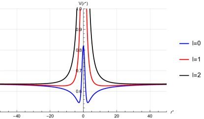
Figure 1: Effective potential of the generalized Bronnikov-Ellis wormhole, for $M/b_{0}=0.25$, $mb_{0}=0.8$ and $\ell=0,1,2$.

On the other hand, Eq. (16) can be written as

$$(2M-r)\left(b_{0}^{2}-r^{2}\right)R^{\prime\prime}(r)+\frac{\left(-3Mb_{0}^{2}+Mr^{2}+b_{0}^{2}r\right)}{r}R^{\prime}(r)+$$

$$\frac{M\left(\left(2m^{2}r^{2}+2\ell^{2}+2\ell-1\right)r^{2}+3b_{0}^{2}\right)-r\left(r^{2}\left(\ell^{2}+\ell+r^{2}(m^{2}-\omega^{2})\right)+b_{0}^{2}\right)}{r^{2}}R(r)=0\,,$$ (21)

which we will solve numerically in order to obtain the QNFs.

IV.1 Quasinormal frequencies

In this section we use the continued fraction method (CFM) to calculate accurately the QNFs for massive scalar fields propagating in the generalized Bronnikov-Ellis wormhole. The CFM was devised by Leaver to compute the QNMs of Schwarzschild and Kerr black holes Leaver:1985ax ; Leaver:1990zz , and improved later by Nollert Nollert:1993zz . It has been used to computed the QNMs in several black holes backgrounds, see for instance Cardoso:2003qd ; Konoplya:2013rxa ; Richartz:2014jla ; Chowdhury:2018pre ; Becar:2022wcj . However, to our knowledge this is the first time that this method is applied to calculate the QNFs in wormhole geometries.

To solve the radial equation it is necessary to specify the boundary conditions. Given the asymptotically flat nature of the wormhole geometry and the fact that the effective potential forms a barrier approaching $V(r^{\ast})\rightarrow m^{2}$ as $r^{\ast}\rightarrow\pm\infty$, we will consider the boundary conditions that demand purely outgoing waves at both infinities. In other words, no waves are coming from either asymptotically flat region Konoplya:2005et ; Bronnikov:2021liv

$$\Psi\sim e^{i\sqrt{\omega^{2}-m^{2}}r^{\ast}}\,,\quad r^{\ast}\rightarrow+\infty\,.$$

$$\Psi\sim e^{-i\sqrt{\omega^{2}-m^{2}}r^{\ast}}\,,\quad r^{\ast}\rightarrow-\infty\,.$$ (22)

However, for the CFM it is more convenient to implement boundary conditions at the throat and at infinity taking into account the symmetry of the potential, as it is explained next. Therefore, the boundary condition that there are only outgoing waves at infinity is satisfied by the radial solution

$$R\sim e^{i\Omega r^{\ast}}\,\,\,\text{as}\,\,\,r^{\ast}\rightarrow\infty\,,$$

where $\Omega=\sqrt{\omega^{2}-m^{2}}$, which can be rewritten as

$$R\sim e^{i\Omega r}r^{iM\omega^{2}/\Omega}\,\,\,\text{as}\,\,\,r\rightarrow\infty\,.$$ (23)

Also, since the potential is symmetric about the throat of the wormhole, which is located at $r_{0}^{\ast}=0$, the solutions will be symmetric or anti-symmetric. Therefore, we impose the following boundary conditions at the throat, $\frac{dR}{dr^{\ast}}\left|{}_{r_{0}^{\ast}}=0\right.$ for the symmetric solutions and $R(r_{0}^{\ast})=0$ for the anti-symmetric solutions. These boundary conditions yields the even and odd overtones, respectively. It is worth mentioning that similar boundary conditions have been applied for other wormhole geometries, where the QNMs were obtained by direct integration of the wave equation Aneesh:2018hlp ; DuttaRoy:2019hij .

It is convenient to consider the following ansatz for the symmetric solutions of the radial equation (IV) which satisfies the desired boundary conditions

$$R(r)=e^{i\Omega r}r^{iM\omega^{2}/\Omega}\sum_{n=0}^{\infty}a_{n}\left(\frac{r-b_{0}}{r}\right)^{n}\,.$$ (24)

So, substituting this expression in the radial equation, the following five-term recurrence relation is satisfied by the expansion coefficients

$$c_{0}(0)a_{1}+c_{1}(0)a_{0}=0\,,$$

$$c_{0}(1)a_{2}+c_{1}(1)a_{1}+c_{2}(1)a_{0}=0\,,$$

$$c_{0}(2)a_{3}+c_{1}(2)a_{2}+c_{2}(2)a_{1}+c_{3}(2)a_{0}=0\,,$$

$$c_{0}(n)a_{n+1}+c_{1}(n)a_{n}+c_{2}(n)a_{n-1}+c_{3}(n)a_{n-2}+c_{4}(n)a_{n-3}=0\,,\,\,n\geq 3\,,$$ (25)

where

$$c_{0}(n) = -(n+1)(2n+1)(b_{0}-2M)\left(m^{2}-\omega^{2}\right)\,,$$

$$c_{1}(n) = b_{0}^{3}\left(m^{2}-\omega^{2}\right)^{2}-ib_{0}^{2}\left(m^{2}-\omega^{2}\right)\left((4n+1)\sqrt{\omega^{2}-m^{2}}-2im^{2}M\right)+b_{0}\Bigg{(}m^{2}\bigg{(}l^{2}+l+n\left(8iM\sqrt{\omega^{2}-m^{2}}+5n+2\right)$$

$$+2iM\sqrt{\omega^{2}-m^{2}}+1\bigg{)}-\omega^{2}\left(l^{2}+l+n\left(4iM\sqrt{\omega^{2}-m^{2}}+5n+2\right)+iM\sqrt{\omega^{2}-m^{2}}+1\right)\Bigg{)}+$$

$$2M\left(-\left(l^{2}+l+n(7n+2)+1\right)\left(m^{2}-\omega^{2}\right)-4iMn\omega^{2}\sqrt{\omega^{2}-m^{2}}-iM\omega^{2}\sqrt{\omega^{2}-m^{2}}\right)\,,$$

$$c_{2}(n) = b_{0}\Bigg{(}\omega^{2}\left(n\left(6iM\sqrt{\omega^{2}-m^{2}}+4n-3\right)-4iM\sqrt{\omega^{2}-m^{2}}+6M^{2}\omega^{2}+1\right)-m^{2}\bigg{(}n\left(12iM\sqrt{\omega^{2}-m^{2}}+4n-3\right)$$

$$-6iM\sqrt{\omega^{2}-m^{2}}+8M^{2}\omega^{2}+1\Bigg{)}\bigg{)}+b_{0}^{2}\left(m^{2}-\omega^{2}\right)\left(2m^{2}M+i(2n-1)\sqrt{\omega^{2}-m^{2}}\right)+M\big{(}(2l(l+1)+n(18n-$$

$$17)+7)\left(m^{2}-\omega^{2}\right)+20iMn\omega^{2}\sqrt{\omega^{2}-m^{2}}-8iM\omega^{2}\sqrt{\omega^{2}-m^{2}}+4M^{2}\omega^{4}\big{)}\,,$$

$$c_{3}(n) = b_{0}\Bigg{(}m^{2}\left(n\left(4iM\sqrt{\omega^{2}-m^{2}}+n-2\right)-5iM\sqrt{\omega^{2}-m^{2}}+4M^{2}\omega^{2}+1\right)-\omega^{2}\bigg{(}n\left(2iM\sqrt{\omega^{2}-m^{2}}+n-2\right)$$

$$-3iM\sqrt{\omega^{2}-m^{2}}+3M^{2}\omega^{2}+1\bigg{)}\Bigg{)}+M\bigg{(}-16iMn\omega^{2}\sqrt{\omega^{2}-m^{2}}+17iM\omega^{2}\sqrt{\omega^{2}-m^{2}}-(2n(5n-11)+13)$$

$$\left(m^{2}-\omega^{2}\right)-6M^{2}\omega^{4}\bigg{)}\,,$$

$$c_{4}(n) = M\left(m^{2}(n-2)(2n-3)+\omega^{2}\left(n\left(4iM\sqrt{\omega^{2}-m^{2}}-2n+7\right)-7iM\sqrt{\omega^{2}-m^{2}}+2M^{2}\omega^{2}-6\right)\right)\,.$$ (26)

On the other hand, for the anti-symmetric solutions it is convenient to define

$$R(r)=(r-b_{0})^{1/2}e^{i\Omega r}r^{iM\omega^{2}/\Omega-1/2}\sum_{n=0}^{\infty}a_{n}\left(\frac{r-b_{0}}{r}\right)^{n}\,,$$ (27)

which incorporates the desired boundary conditions. Thus, substituting this expression in the radial equation, also a five-term recurrence relation (IV.1) is satisfied by the expansion coefficients, but now the coefficients are given by

$$c_{0}(n) = -4(n+1)(2n+3)\left(b_{0}-2M\right)\left(m^{2}-\omega^{2}\right)\,,$$

$$c_{1}(n) = b_{0}\Bigg{(}m^{2}\left(4l(l+1)+4n\left(8iM\sqrt{\omega^{2}-m^{2}}+5n+7\right)+24iM\sqrt{\omega^{2}-m^{2}}+13\right)-\omega^{2}\bigg{(}4l(l+1)+$$

$$4n\left(4iM\sqrt{\omega^{2}-m^{2}}+5n+7\right)+12iM\sqrt{\omega^{2}-m^{2}}+13\bigg{)}\Bigg{)}-4b_{0}^{2}\left(m^{2}-\omega^{2}\right)\left(2m^{2}M+i(4n+3)\sqrt{\omega^{2}-m^{2}}\right)+$$

$$4b_{0}^{3}\left(m^{2}-\omega^{2}\right)^{2}+2M\left(-(4l(l+1)+4n(7n+9)+15)\left(m^{2}-\omega^{2}\right)-16iMn\omega^{2}\sqrt{\omega^{2}-m^{2}}-12iM\omega^{2}\sqrt{\omega^{2}-m^{2}}\right)\,,$$

$$c_{2}(n) = -2b_{0}m^{2}\left(2n\left(12iM\sqrt{\omega^{2}-m^{2}}+4n+1\right)+16M^{2}\omega^{2}+1\right)+2b_{0}\omega^{2}\bigg{(}2n\left(6iM\sqrt{\omega^{2}-m^{2}}+4n+1\right)-$$

$$2iM\sqrt{\omega^{2}-m^{2}}+12M^{2}\omega^{2}+1\bigg{)}+8b_{0}^{2}\left(m^{2}-\omega^{2}\right)\left(m^{2}M+in\sqrt{\omega^{2}-m^{2}}\right)+4M\bigg{(}\left(2l(l+1)+18n^{2}+n+3\right)$$

$$\left(m^{2}-\omega^{2}\right)+20iMn\omega^{2}\sqrt{\omega^{2}-m^{2}}+2iM\omega^{2}\sqrt{\omega^{2}-m^{2}}+4M^{2}\omega^{4}\bigg{)}\,,$$

$$c_{3}(n) = b_{0}\Bigg{(}m^{2}\left(4n\left(4iM\sqrt{\omega^{2}-m^{2}}+n-1\right)+4M\left(4M\omega^{2}-3i\sqrt{\omega^{2}-m^{2}}\right)+1\right)-\omega^{2}\bigg{(}4n\left(2iM\sqrt{\omega^{2}-m^{2}}+n-1\right)$$

$$-8iM\sqrt{\omega^{2}-m^{2}}+12M^{2}\omega^{2}+1\bigg{)}\Bigg{)}+2M\bigg{(}-32iMn\omega^{2}\sqrt{\omega^{2}-m^{2}}+18iM\omega^{2}\sqrt{\omega^{2}-m^{2}}-(4n(5n-6)+9)$$

$$\left(m^{2}-\omega^{2}\right)-12M^{2}\omega^{4}\bigg{)}\,,$$

$$c_{4}(n) = 4M\left(m^{2}(n-1)(2n-3)+\omega^{2}\left(n\left(4iM\sqrt{\omega^{2}-m^{2}}-2n+5\right)-5iM\sqrt{\omega^{2}-m^{2}}+2M^{2}\omega^{2}-3\right)\right)\,.$$

Then, after applying Gaussian elimination twice, the original five-term recurrence relations (IV.1) can be simplified to a three-term relation, taking on the following concise form

$$\alpha_{0}a_{1}+\beta_{0}a_{0} = 0\,,$$

$$\alpha_{n}a_{n+1}+\beta_{n}a_{n}+\gamma_{n}a_{n-1} = 0\,,\,\,\,\,n=1,2,...$$

We skip providing the explicit expressions for $\alpha_{n}$, $\beta_{n}$ and $\gamma_{n}$ of the final three-term recurrence relations. Now, according to Leaver Leaver:1985ax ; Leaver:1990zz , the recursion coefficients must satisfy the following continued fraction relation for the convergence of the series

$$\beta_{0}-\frac{\alpha_{0}\gamma_{1}}{\beta_{1}-}\frac{\alpha_{1}\gamma_{2}}{\beta_{2}-}\cdots\frac{\alpha_{n}\gamma_{n+1}}{\beta_{n+1}-}\cdots=0\,,$$ (28)

The continued fraction must be truncated at some large index $N$ and the QNFs are obtained solving this equation numerically. In the following figures we show the behaviour of $Re(\omega)b_{0}$ and $-Im(\omega)b_{0}$ for massive scalar field as a function of $mb_{0}$ using the CFM, for the fundamental mode, see Fig. 2, and 4, and the first overtone, see Fig. 3, and 5.

For the fundamental QNFs ($n=0$), we can observe an inverted behaviour of $Im(\omega)b_{0}$, that is, when $mb_{0}>m_{c}b_{0}$, $Im(\omega)b_{0}$ increases with $\ell$, representing an anomalous decay rate of the QNMs. Conversely, for $mb_{0}<m_{c}b_{0}$, $Im(\omega)b_{0}$ decreases with increasing $\ell$ for $n\geq\ell$. The critical value $m_{c}b_{0}$ rises with an increase in the parameter $M/b_{0}$, and the frequency of the oscillation increases with both the angular number and the parameter $mb_{0}$. The frequencies all have a negative imaginary part, which means that the propagation of massive scalar fields is stable in this background. Some numerical values of the QNFs obtained with CFM are in appendix A. Moreover, in appendix B we compare the fundamental QNFs and the first overtone using the CFM and the WKB approximation, and we see a poor agreement with the fundamental QNF but a good agreement for high values of $\ell$ as expected, because it is known that the WKB method only yields accurate results for high values of $\ell$ and for $\ell>n$.

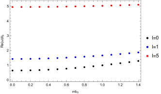
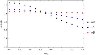
Figure 2: The behaviour of $Re(\omega)b_{0}$ and $-Im(\omega)b_{0}$ for massive scalar field as a function of $mb_{0}$ for the generalized Bronnikov-Ellis wormhole with $M/b_{0}=0.1$, $n=0$ (fundamental frequency), and $\ell=0,1,5$ using the CFM.

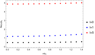
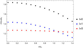
Figure 3: The behaviour of $Re(\omega)b_{0}$ and $-Im(\omega)b_{0}$ for massive scalar field as a function of $mb_{0}$ for the generalized Bronnikov-Ellis wormhole with $M/b_{0}=0.1$, $n=1$ (first overtone), and $\ell=0,1,5$ using the CFM.

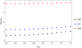
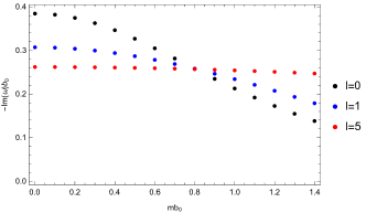
Figure 4: The behaviour of $Re(\omega)b_{0}$ and $-Im(\omega)b_{0}$ for massive scalar field as a function of $mb_{0}$ for the generalized Bronnikov-Ellis wormhole with $M/b_{0}=0.25$, $n=0$ (fundamental frequency), and $\ell=0,1,5$ using the CFM.

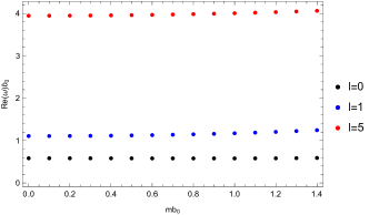
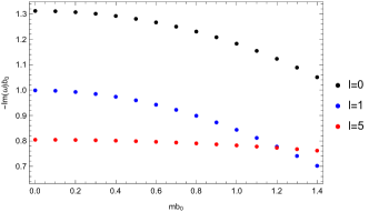
Figure 5: The behaviour of $Re(\omega)b_{0}$ and $-Im(\omega)b_{0}$ for massive scalar field as a function of $mb_{0}$ for the generalized Bronnikov-Ellis wormhole with $M/b_{0}=0.25$, $n=1$ (first overtone), and $\ell=0,1,5$ using the CFM.

IV.2 Bound States

In this section we calculate the bound states of massive scalar fields around the generalized Bronnikov-Ellis wormhole using the CFM, which are possible due to the effective potential allows potential wells, see Fig. (1). It is worth to mention that the boundary conditions are different to that of QNMs. In this case we must considering evanescent waves at spatial infinity; therefore, the radial solution that satisfied the boundary condition at infinity is given by

$$R\sim e^{-\Omega r}r^{M\omega^{2}/\Omega}\,\,\,\text{as}\,\,\,r\rightarrow\infty\,,$$ (29)

where $\Omega=\sqrt{m^{2}-\omega^{2}}$. Generally, in a quantum system with a potential well, there are only a few bound states, the number of which depends on the potential parameters. In several cases, there exists only a single bound state. Thus, we just consider the first bound state which is described by the symmetric solution. Therefore, we consider the following ansatz for the solution to the radial equation (IV) which satisfies the desired boundaries conditions

$$R(r)=e^{-\Omega r}r^{M\omega^{2}/\Omega}\sum_{n=0}^{\infty}a_{n}\left(\frac{r-b_{0}}{r}\right)^{n}\,.$$ (30)

Then, substituting this expression in the radial equation, the following seven-term recurrence relation is satisfied by the expansion coefficients

$$c_{0}(0)a_{1}+c_{1}(0)a_{0}=0\,,$$

$$c_{0}(1)a_{2}+c_{1}(1)a_{1}+c_{2}(1)a_{0}=0\,,$$

$$c_{0}(2)a_{3}+c_{1}(2)a_{2}+c_{2}(2)a_{1}+c_{3}(2)a_{0}=0\,,$$

$$c_{0}(3)a_{4}+c_{1}(3)a_{3}+c_{2}(3)a_{2}+c_{3}(3)a_{1}+c_{4}(3)a_{0}=0\,,$$

$$c_{0}(4)a_{5}+c_{1}(4)a_{4}+c_{2}(4)a_{3}+c_{3}(4)a_{2}+c_{4}(4)a_{1}+c_{5}(4)a_{0}=0$$

$$c_{0}(n)a_{n+1}+c_{1}(n)a_{n}+c_{2}(n)a_{n-1}+c_{3}(n)a_{n-2}+c_{4}(n)a_{n-3}+c_{5}(n)a_{n-4}+c_{6}(n)a_{n-5}=0\,,n\geq 5\,,$$ (31)

where

$$c_{0}(n) = (n+1)(2n+1)\left(b_{0}-2M\right)\left(m^{2}-\omega^{2}\right)\,,$$

$$c_{1}(n) = b_{0}\Bigg{(}\omega^{2}\left(l^{2}+l-4Mn\sqrt{m^{2}-\omega^{2}}-M\sqrt{m^{2}-\omega^{2}}+9n^{2}+1\right)-m^{2}\bigg{(}l^{2}+l-8Mn\sqrt{m^{2}-\omega^{2}}-2M\sqrt{m^{2}-\omega^{2}}$$

$$+9n^{2}+1\bigg{)}\Bigg{)}-b_{0}^{2}\left(m^{2}-\omega^{2}\right)\left((4n+1)\sqrt{(m-\omega)(m+\omega)}-2m^{2}M\right)+b_{0}^{3}\left(-\left(m^{2}-\omega^{2}\right)^{2}\right)+2M\bigg{(}(l^{2}+l$$

$$+11n^{2}+1)\left(m^{2}-\omega^{2}\right)-4Mn\omega^{2}\sqrt{m^{2}-\omega^{2}}-M\omega^{2}\sqrt{m^{2}-\omega^{2}}\bigg{)}\,,$$

$$c_{2}(n) = 2b_{0}\Bigg{(}m^{2}\left(l^{2}+l+2n\left(-7M\sqrt{m^{2}-\omega^{2}}+4n-6\right)+9M\sqrt{m^{2}-\omega^{2}}+4M^{2}\omega^{2}+6\right)-\omega^{2}\bigg{(}l^{2}+l+$$

$$n\left(-7M\sqrt{m^{2}-\omega^{2}}+8n-12\right)+5M\sqrt{m^{2}-\omega^{2}}+3M^{2}\omega^{2}+6\bigg{)}\Bigg{)}+b_{0}^{2}\left(m^{2}-\omega^{2}\right)\bigg{(}(10n-7)$$

$$\sqrt{(m-\omega)(m+\omega)}-6m^{2}M\bigg{)}+2b_{0}^{3}\left(m^{2}-\omega^{2}\right)^{2}+M\bigg{(}-(6l(l+1)+25n(2n-3)+37)\left(m^{2}-\omega^{2}\right)$$

$$+36Mn\omega^{2}\sqrt{m^{2}-\omega^{2}}-20M\omega^{2}\sqrt{m^{2}-\omega^{2}}-4M^{2}\omega^{4}\bigg{)}\,,$$

$$c_{3}(n) = b_{0}\Bigg{(}\omega^{2}\left(l^{2}+l+2n\left(-9M\sqrt{m^{2}-\omega^{2}}+7n-21\right)+15M\left(2\sqrt{m^{2}-\omega^{2}}+M\omega^{2}\right)+34\right)-m^{2}\bigg{(}l^{2}+l$$

$$-6n\left(6M\sqrt{m^{2}-\omega^{2}}+7\right)+55M\sqrt{m^{2}-\omega^{2}}+20M^{2}\omega^{2}+14n^{2}+34\bigg{)}\Bigg{)}+b_{0}^{2}\left(m^{2}-\omega^{2}\right)\bigg{(}6m^{2}M+(13-8n)$$

$$\sqrt{(m-\omega)(m+\omega)}\bigg{)}+b_{0}^{3}\left(-\left(m^{2}-\omega^{2}\right)^{2}\right)+M\bigg{(}3(2l(l+1)+20(n-3)n+49)\left(m^{2}-\omega^{2}\right)-$$

$$64Mn\omega^{2}\sqrt{m^{2}-\omega^{2}}+87M\omega^{2}\sqrt{m^{2}-\omega^{2}}+14M^{2}\omega^{4}\bigg{)}\,,$$

$$c_{4}(n) = b_{0}\Bigg{(}m^{2}\left(n\left(-20M\sqrt{m^{2}-\omega^{2}}+6n-27\right)+16M\left(3\sqrt{m^{2}-\omega^{2}}+M\omega^{2}\right)+31\right)-\omega^{2}\bigg{(}n(-10M\sqrt{m^{2}-\omega^{2}}+$$

$$6n-27)+26M\sqrt{m^{2}-\omega^{2}}+12M^{2}\omega^{2}+31\bigg{)}\Bigg{)}+b_{0}^{2}\left(m^{2}-\omega^{2}\right)\left((2n-5)\sqrt{(m-\omega)(m+\omega)}-2m^{2}M\right)+$$

$$M\left(-(2l(l+1)+20n(2n-9)+209)\left(m^{2}-\omega^{2}\right)+56Mn\omega^{2}\sqrt{m^{2}-\omega^{2}}-121M\omega^{2}\sqrt{m^{2}-\omega^{2}}-18M^{2}\omega^{4}\right)\,,$$

$$c_{5}(n) = b_{0}\Bigg{(}\omega^{2}\left(n\left(-2M\sqrt{m^{2}-\omega^{2}}+n-6\right)+7M\sqrt{m^{2}-\omega^{2}}+3M^{2}\omega^{2}+9\right)-m^{2}\bigg{(}n\left(-4M\sqrt{m^{2}-\omega^{2}}+n-6\right)$$

$$+13M\sqrt{m^{2}-\omega^{2}}+4M^{2}\omega^{2}+9\bigg{)}\Bigg{)}+M\bigg{(}-24Mn\omega^{2}\sqrt{m^{2}-\omega^{2}}+71M\omega^{2}\sqrt{m^{2}-\omega^{2}}+(14(n-6)n+127)$$

$$\left(m^{2}-\omega^{2}\right)+10M^{2}\omega^{4}\bigg{)}\,,$$

$$c_{6}(n) = M\left(\omega^{2}\left(n\left(4M\sqrt{m^{2}-\omega^{2}}+2n-15\right)-15M\sqrt{m^{2}-\omega^{2}}-2M^{2}\omega^{2}+28\right)-m^{2}(n-4)(2n-7)\right)\,.$$

Then, after applying Gaussian elimination four times, the original seven-term recurrence relations (IV.2) can be simplified to a three-term relation, taking on the following concise form

$$\alpha_{0}a_{1}+\beta_{0}a_{0} = 0\,,$$

$$\alpha_{n}a_{n+1}+\beta_{n}a_{n}+\gamma_{n}a_{n-1} = 0\,,\,\,\,\,n=1,2,...$$

We skip providing the explicit expressions for $\alpha_{n}$, $\beta_{n}$ and $\gamma_{n}$ of the final three-term recurrence relations.

Now, according to Leaver Leaver:1985ax ; Leaver:1990zz , the recursion coefficients must satisfy the following continued fraction relation for the convergence of the series

$$\beta_{0}-\frac{\alpha_{0}\gamma_{1}}{\beta_{1}-}\frac{\alpha_{1}\gamma_{2}}{\beta_{2}-}\cdots\frac{\alpha_{n}\gamma_{n+1}}{\beta_{n+1}-}\cdots=0\,,$$ (32)

and the continued fraction must be truncated at some large index $N$. The bound states frequencies are obtained solving this equation numerically. In Table 1, we show some values of the lowest bound states frequencies $\omega b_{0}$ for scalar perturbations using the CFM. We observe that the oscillation frequency increases when the mass parameter $mb_{0}$ increases and when the angular number $\ell$ increases.

Table 1: The lowest bound states frequencies $\omega b_{0}$ for scalar perturbations for the generalized Bronnikov-Ellis wormhole with $M/b_{0}=0.25$, $\ell=0,1$, and several values of the mass of the scalar field using the CFM.

$\ell$	$mb_{0}=0.4$	$mb_{0}=0.8$	$mb_{0}=1.2$	$mb_{0}=1.6$
0	0.39948020	0.77659459	1.10626752	1.40450402
1	0.39949541	0.79583960	1.18498187	1.55693415
$\ell$	$mb_{0}=2$	$mb_{0}=2.4$	$mb_{0}=2.8$	$mb_{0}=3.2$
0	1.69213119	1.97599183	2.25838693	2.54020128
1	1.87946685	2.16141735	2.43284661	2.70240221

V f(R) gravity wormhole

In the framework of $f(R)$ modified gravity, a generalization of the Ellis drainhole solution was found in Karakasis:2021tqx by considering a phantom scalar field with a self-interacting potential. The solution is given by

$$\Phi(r)=0\,,\,\,b(r)=2r-\mu^{2}r^{3}\,,\,\,\phi(r)=\sqrt{6}\frac{\sqrt{A}}{r}\,,\,\,V(\phi)=\frac{1}{2}\mu^{2}\phi^{2}\,.\,\,$$ (33)

The condition $\frac{b(r)}{r}\leq 1$ reduces to $\mu^{2}r^{2}\geq 1$, which holds for all $r$ within the interval $[\frac{1}{\mu},+\infty)$. Also, the condition $\frac{b(r)}{r}=1$ yields the throat location at $r_{th}=\frac{1}{\mu}$, where $\mu$ can be interpreted as the mass of the phantom scalar field. Furthermore, the flare-out condition $b^{\prime}(r)<\frac{b(r)}{r}$ results in $\mu^{2}r^{2}>0$, which is satisfied for every $r>0$ and $\mu\neq 0$. Also, it can be easily verified that $b^{\prime}(r_{th})=-1$, ensuring that the relation $b^{\prime}(r_{th})\leq 1$ always holds true.

The fundamental characteristics of the solution highlight the impact of the phantom scalar field on both the scalar curvature and the throat’s size. As the strength of the scalar field intensifies, the resulting wormholes exhibit larger throat radii, consequently diminishing the curvature in the vicinity of the throat. We direct the reader to Ref. Karakasis:2021tqx for a comprehensive review of the solution.

V.1 Analytical QNFs of f(R) gravity wormhole

In this section we study the propagation of a probe scalar field in the $f(R)$ wormhole geometry, with a particular focus on studying its stability through the QNFs. In this case the Klein-Gordon equation, considering the following separation of variables

$$\Psi(t,r,\theta,\phi)=e^{-i\omega t}\>\frac{R(r)}{r}\>Y_{\ell}(\Omega)\,,$$ (34)

can be written as a one-dimensional Schrödinger-like equation

$$\frac{\mathrm{d}^{2}R}{\mathrm{d}r^{\ast}{}^{2}}+[\omega^{2}-V(r^{\ast})]R=0\,,$$ (35)

where $\omega$ is the unknown frequency, while $Y_{\ell}(\Omega)$ are the spherical harmonics, and $r^{\ast}$ is the well-known tortoise coordinate, i.e.,

$$r^{\ast}\equiv\int\frac{\mathrm{d}r}{e^{\Phi}\sqrt{1-\frac{b(r)}{r}}}\,.$$ (36)

The effective potential governing scalar perturbations for the $f(R)$ gravity wormhole reads

$$V(r)=\frac{\ell(\ell+1)}{r^{2}}+\mu^{2}+m^{2}\,,$$ (37)

which we plot in Fig. 6. We observe that the effective potential is symmetric about the throat of the wormhole and takes the form of a barrier for $\ell\neq 0$, with the barrier magnitude increasing with $\ell$. However, it does not allow wells, consequently precluding the support for bound states.

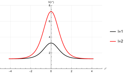
Figure 6: Effective potential for $\mu=1$, $m=0.5$ and $\ell=1,2$.

It is worth noticing that when $\ell=0$ the effective potential is constant. Consequently, the solution of the radial function is given by $R=C_{1}e^{i\sqrt{\omega^{2}-\mu^{2}-m^{2}}r^{*}}+C_{2}e^{-i\sqrt{\omega^{2}-\mu^{2}-m^{2}}r^{*}}$. Imposing the condition of purely outgoing waves at both infinities leads to the conclusion that $C_{1}=C_{2}=0$, resulting in $R=0$ for this particular case.

Now we consider the case $\ell\neq 0$. The radial equation can be written as

$$(1-\tilde{r}^{2})\frac{d^{2}}{d\tilde{r}^{2}}R(\tilde{r})-\tilde{r}\frac{d}{d\tilde{r}}R(\tilde{r})+\left(\frac{\ell(\ell+1)}{\tilde{r}^{2}}-\tilde{\omega}^{2}+1+\tilde{m}^{2}\right)R(\tilde{r})=0\,,$$ (38)

where we have defined a dimensionless coordinate $\tilde{r}=\mu r$, $\tilde{m}=m/\mu$ and $\tilde{\omega}=\omega/\mu$. The radial equation can be analytically solved by expressing it in terms of hypergeometric functions

$$R(\tilde{r}) = C_{1}\tilde{r}^{\frac{1}{2}(1-\sqrt{1-4\ell(\ell+1)})}\,_{2}F_{1}\Bigg{(}\frac{1}{4}-\frac{1}{4}\sqrt{1-4\ell(\ell+1)}-\frac{\sqrt{1+\tilde{m}^{2}-\tilde{\omega}^{2}}}{2},\frac{1}{4}-\frac{1}{4}\sqrt{1-4\ell(\ell+1)}+\frac{\sqrt{1+\tilde{m}^{2}-\tilde{\omega}^{2}}}{2},$$ (39)

$$1-\frac{1}{2}\sqrt{1-4\ell(\ell+1)},\tilde{r}^{2}\Bigg{)}+C_{2}r^{\frac{1}{2}(1+\sqrt{1-4\ell(\ell+1)})}\,_{2}F_{1}\Bigg{(}\frac{1}{4}+\frac{1}{4}\sqrt{1-4\ell(\ell+1)}-\frac{\sqrt{1+\tilde{m}^{2}-\tilde{\omega}^{2}}}{2},$$

$$\frac{1}{4}+\frac{1}{4}\sqrt{1-4\ell(\ell+1)}+\frac{\sqrt{1+\tilde{m}^{2}-\tilde{\omega}^{2}}}{2},1+\frac{1}{2}\sqrt{1-4\ell(\ell+1)},\tilde{r}^{2}\Bigg{)}\,,$$

where $\,{}_{2}F_{1}$ is the Gaussian Hypergeometric function.

Since the potential is symmetric about the throat of the wormhole, which is located at $r_{0}^{\ast}=0$, the solutions will be symmetric or anti-symmetric. Therefore, we impose the following boundary conditions at the throat, $\frac{dR}{dr^{\ast}}\left|{}_{r_{0}^{\ast}}=0\right.$ for the symmetric solutions and $R(r_{0}^{\ast})=0$ for the anti-symmetric solutions. These boundary conditions yields the even and odd overtones, respectively. Similar boundary conditions have been applied for other wormhole geometries, where the QNMs were obtained by direct integration of the wave equation Aneesh:2018hlp ; DuttaRoy:2019hij . So, for the symmetric solutions we impose the condition at the throat $\frac{dR}{dr^{\ast}}\left|{}_{r_{0}^{\ast}}\right.=\frac{dR}{d\tilde{r}}\sqrt{1-\frac{b(\tilde{r})}{\tilde{r}}}\left|{}_{\tilde{r}=1}\right.=0$ , which yields

$$C_{1}=C_{2}\rho\frac{\Gamma[1+\alpha_{+}]\Gamma[1+\alpha_{-}]\Gamma\left[1+\frac{1}{2}\sqrt{1-4\ell(\ell+1)}\right]}{\Gamma[1+\gamma_{-}]\Gamma[1+\gamma_{+}]\Gamma\left[1-\frac{1}{2}\sqrt{1-4\ell(\ell+1)}\right]}\,,$$

where

$$\rho=\frac{-2(2-\sqrt{1-4\ell(\ell+1)})\tilde{m}^{2}-3+4\tilde{\omega}^{2}+\sqrt{1-4\ell(\ell+1)}((3+2\ell(\ell+1))-2\tilde{\omega}^{2})}{\left(2\tilde{m}^{2}+(1+2\ell(\ell+1)+\sqrt{1-4\ell(\ell+1)})-2\tilde{\omega}^{2}\right)(2-\sqrt{1-4\ell(\ell+1)})}\,,$$

and the asymptotic behaviour of the solutions is

$$R(\tilde{r})\sim C_{2}\tilde{r}^{-i\sqrt{\tilde{\omega}^{2}-1-\tilde{m}^{2}}}\Gamma\left[-\sqrt{1+\tilde{m}^{2}-\tilde{\omega}^{2}}\right]\Gamma\left[1+\frac{1}{2}\sqrt{1-4\ell(\ell+1)}\right]\Bigg{(}(-1)^{-\alpha_{+}}\rho(\alpha_{-}/\gamma_{-})\frac{\Gamma[1+\alpha_{+}]}{\Gamma[\beta_{-}]\Gamma[1+\gamma_{+}]}$$ (40)

$$+\frac{(-1)^{-\gamma_{+}}}{\Gamma[\delta_{-}]}\Bigg{)}\frac{1}{\Gamma[\gamma_{-}]}+C_{2}\tilde{r}^{i\sqrt{\tilde{\omega}^{2}-1-\tilde{m}^{2}}}\Gamma\left[\sqrt{1+\tilde{m}^{2}-\tilde{\omega}^{2}}\right]\Gamma\left[1+\frac{1}{2}\sqrt{1-4\ell(\ell+1)}\right]$$

$$\Bigg{(}(-1)^{-\alpha_{-}}\rho(\alpha_{+}/\gamma_{+})\frac{\Gamma[1+\alpha_{-}]}{\Gamma[\beta_{+}]\Gamma[1+\gamma_{-}]}+\frac{(-1)^{-\gamma_{-}}}{\Gamma[\delta_{+}]}\Bigg{)}\frac{1}{\Gamma[\gamma_{+}]}\,,$$

where we have defined

$$\alpha_{\pm} = \frac{1}{4}-\frac{\sqrt{1-4\ell(\ell+1)}}{4}\pm\frac{\sqrt{1+\tilde{m}^{2}-\tilde{\omega}^{2}}}{2}\,,\,\,\,\,\beta_{\pm}=\frac{3}{4}-\frac{\sqrt{1-4\ell(\ell+1)}}{4}\pm\frac{\sqrt{1+\tilde{m}^{2}-\tilde{\omega}^{2}}}{2}\,,$$

$$\gamma_{\pm} = \frac{1}{4}+\frac{\sqrt{1-4\ell(\ell+1)}}{4}\pm\frac{\sqrt{1+\tilde{m}^{2}-\tilde{\omega}^{2}}}{2}\,,\,\,\,\,\delta_{\pm}=\frac{3}{4}+\frac{\sqrt{1-4\ell(\ell+1)}}{4}\pm\frac{\sqrt{1+\tilde{m}^{2}-\tilde{\omega}^{2}}}{2}\,.$$

Now, in accordance with the boundary condition of purely outgoing waves at spatial infinity, i.e. $R\sim r^{i\sqrt{\tilde{\omega}^{2}-1-\tilde{m}^{2}}}$, we set

$$\gamma_{-}=\frac{1}{4}+\frac{\sqrt{1-4\ell(\ell+1)}}{4}-\frac{\sqrt{1+\tilde{m}^{2}-\tilde{\omega}^{2}}}{2}=-n\,\,\,\,\,\,\,\,n=0,1,...$$ (41)

Therefore, the QNFs for even overtones yield

$$\tilde{\omega}=\frac{1}{\sqrt{2}}\left(\eta+\left(\eta^{2}+\frac{1}{4}(-1+4\ell(\ell+1))(1+4n)^{2}\right)^{1/2}\right)^{1/2}-i\frac{\left(-1+4\ell(\ell+1)\right)^{1/2}(1+4n)}{2\sqrt{2}\left(\eta+\left(\eta^{2}+\frac{1}{4}(-1+4\ell(\ell+1))(1+4n)^{2}\right)^{1/2}\right)^{1/2}}\,,$$ (42)

where $\eta\equiv\frac{1}{2}(1+2\ell(\ell+1)-4n(1+2n))+\tilde{m}^{2}$  .

On the other hand, we impose the condition at the throat $R(1)=0$ as a boundary condition for the antisymmetric solutions, leading to the expression

$$C_{1}=-C_{2}\frac{\Gamma[\beta_{+}]\Gamma[\beta_{-}]\Gamma\left[1+\frac{1}{2}\sqrt{1-4\ell(\ell+1)}\right]}{\Gamma[\gamma_{+}]\Gamma[\gamma_{-}]\Gamma\left[1-\frac{1}{2}\sqrt{1-4\ell(\ell+1)}\right]}\,.$$

Thus, the asymptotic behaviour of the solutions is

$$R(\tilde{r})\sim C_{2}\tilde{r}^{-i\sqrt{\tilde{\omega}^{2}-1-\tilde{m}^{2}}}\Gamma\left[-\sqrt{1+\tilde{m}^{2}-\tilde{\omega}^{2}}\right]\Gamma\left[1+\frac{1}{2}\sqrt{1-4\ell(\ell+1)}\right]\Bigg{(}-(-1)^{-\alpha_{+}}\frac{\Gamma[\beta_{+}]}{\Gamma[\alpha_{-}]\Gamma[\delta_{+}]}$$ (43)

$$+\frac{(-1)^{-\gamma_{+}}}{\Gamma[\gamma_{-}]}\Bigg{)}\frac{1}{\Gamma[\delta_{-}]}+C_{2}\tilde{r}^{i\sqrt{\tilde{\omega}^{2}-1-\tilde{m}^{2}}}\Gamma\left[\sqrt{1+\tilde{m}^{2}-\tilde{\omega}^{2}}\right]\Gamma\left[1+\frac{1}{2}\sqrt{1-4\ell(\ell+1)}\right]$$

$$\Bigg{(}-(-1)^{-\alpha_{-}}\frac{\Gamma[\beta_{-}]}{\Gamma[\alpha_{+}]\Gamma[\delta_{-}]}+\frac{(-1)^{-\gamma_{-}}}{\Gamma[\gamma_{+}]}\Bigg{)}\frac{1}{\Gamma[\delta_{+}]}\,.$$

Now, in accordance with the boundary condition of purely outgoing waves at spatial infinity, i.e. $R\sim r^{i\sqrt{\tilde{\omega}^{2}-1-\tilde{m}^{2}}}$, we set

$$\delta_{-}=\frac{3}{4}+\frac{\sqrt{1-4\ell(\ell+1)}}{4}-\frac{\sqrt{1+\tilde{m}^{2}-\tilde{\omega}^{2}}}{2}=-n\,\,\,\,\,\,\,\,n=0,1,...$$ (44)

and the QNFs for odd overtones yield

$$\tilde{\omega}=\frac{1}{\sqrt{2}}\left(\eta^{\prime}+\left(\eta^{\prime 2}+\frac{1}{4}(-1+4\ell(\ell+1))(3+4n)^{2}\right)^{1/2}\right)^{1/2}-i\frac{\left(-1+4\ell(\ell+1)\right)^{1/2}(3+4n)}{2\sqrt{2}\left(\eta^{\prime}+\left(\eta^{\prime 2}+\frac{1}{4}(-1+4\ell(\ell+1))(3+4n)^{2}\right)^{1/2}\right)^{1/2}}\,,$$ (45)

where $\eta^{\prime}\equiv\frac{1}{2}(-3+2\ell(\ell+1)-4n(3+2n))+\tilde{m}^{2}$.

Finally, the QNFs given by Eq. (42) for even overtones and Eq. (45) for odd overtones, can be succinctly expressed in a unified formula as

$$\tilde{\omega}=\frac{1}{\sqrt{2}}\left(\eta^{\prime\prime}+\left(\eta^{\prime\prime 2}+\frac{1}{4}(-1+4\ell(\ell+1))(1+2n)^{2}\right)^{1/2}\right)^{1/2}-i\frac{\left(-1+4\ell(\ell+1)\right)^{1/2}(1+2n)}{2\sqrt{2}\left(\eta^{\prime\prime}+\left(\eta^{\prime\prime 2}+\frac{1}{4}(-1+4\ell(\ell+1))(1+2n)^{2}\right)^{1/2}\right)^{1/2}}\,,$$ (46)

where $\eta^{\prime\prime}\equiv\frac{1}{2}(1+2\ell(\ell+1)-2n(1+n))+\tilde{m}^{2}$ and $n=0,1,\dots$. In Figs. 7 and 8 we plot the behaviour of $Re(\tilde{\omega})$, and $-Im(\tilde{\omega})$ as a function of $\tilde{m}$ by using the analytical expression (46) for $n=0$ and $n=1$, respectively. We can observe that the modes with the lowest angular number $\ell$ exhibit the longest lifetimes, both for the fundamental and the first overtone, and the decay rate decreases with $\tilde{m}$. Additionally, the frequency of oscillation increases with higher values of the parameter $\tilde{m}$ and the angular momentum $\ell$.

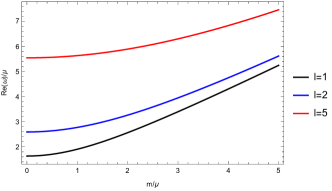
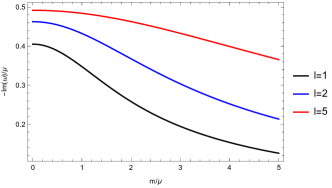
Figure 7: The behaviour of $Re(\omega)/\mu$ (left panel), and $-Im(\omega)/\mu$ (right panel) as a function of $m/\mu$ for different values of $\ell$ and $n=0$.

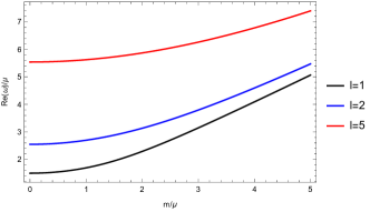
Figure 8: The behaviour of $Re(\omega)/\mu$ (left panel), and $-Im(\omega)/\mu$ (right panel) as a function of $m/\mu$ for different values of $\ell$ and $n=1$.

All the frequencies exhibit a negative imaginary part, indicating the stability of the propagation of massive scalar fields in this background. Defining $L=\sqrt{\ell(\ell+1)}$ and considering high values of $L$, this expression can be approximated to

$$\tilde{\omega}\approx L+\frac{3+4\tilde{m}^{2}}{8L}-i\left(\frac{1}{2}+n-\frac{(1+\tilde{m}^{2})(1+2n)}{4L^{2}}\right)\,.$$ (47)

As we will see in the next subsection this result match with the QNFs obtained via the third order WKB method.

V.2 WKB Method

In this section, we employ the Wentzel-Kramers-Brillouin (WKB) approximation method, first introduced by Mashhoon Mashhoon and later developed by Schutz and Iyer Schutz:1985km . This approach allows us to gain insights into the behaviour of QNFs in the eikonal limit as $\ell\rightarrow\infty$. Our aim is to validate and complement the analytical results obtained in the previous section using an alternative method. Iyer and Will computed the third order correction Iyer:1986np , which was subsequently extended to the sixth order Konoplya:2003ii , and recently up to the 13th order Matyjasek:2017psv , see also Konoplya:2019hlu .

This method has been used to determine the QNFs for asymptotically flat and asymptotically de Sitter black holes. This is due to the WKB method can be used for effective potentials which have the form of potential barriers that approach to a constant value at the horizon and spatial infinity Konoplya:2011qq . The QNMs are determined by the behaviour of the effective potential near its maximum value $V(r^{*}_{max})$. The Taylor series expansion of the potential around its maximum is given by

$$V(r^{*})=V(r^{*}_{max})+\sum_{i=2}^{\infty}\frac{V^{(i)}}{i!}(r^{*}-r^{*}_{max})^{i}\,,$$ (48)

where

$$V^{(i)}=\frac{d^{i}}{dr^{*i}}V(r^{*})|_{r^{*}=r^{*}_{max}}\,,$$ (49)

corresponds to the $i$-th derivative of the potential with respect to $r^{*}$ evaluated at the position of the maximum of the potential $r^{*}_{max}$. Using the WKB approximation up to third order beyond the eikonal limit, the QNFs are given by the following expression Hatsuda:2019eoj

$$\omega^{2} = V(r^{*}_{max})-2iU\,,$$ (50)

where

$$U = N\sqrt{-V^{(2)}/2}+\frac{i}{64}\left(-\frac{1}{9}\frac{V^{(3)2}}{V^{(2)2}}(7+60N^{2})+\frac{V^{(4)}}{V^{(2)}}(1+4N^{2})\right)+\frac{N}{2^{3/2}288}\Bigg{(}\frac{5}{24}\frac{V^{(3)4}}{(-V^{(2)})^{9/2}}(77+188N^{2})$$

$$+\frac{3}{4}\frac{V^{(3)2}V^{(4)}}{(-V^{(2)})^{7/2}}(51+100N^{2})+\frac{1}{8}\frac{V^{(4)2}}{(-V^{(2)})^{5/2}}(67+68N^{2})+\frac{V^{(3)}V^{(5)}}{(-V^{(2)})^{5/2}}(19+28N^{2})+\frac{V^{(6)}}{(-V^{(2)})^{3/2}}(5+4N^{2})\Bigg{)}\,,$$

and $N=n+1/2$, with $n=0,1,2,\dots$, is the overtone number. Now, defining $L^{2}=\ell(\ell+1)$, we find that for large values of $L$, the QNFs are approximately given by

$$\tilde{\omega}\approx\omega_{1}L+\omega_{0}+\omega_{-1}L^{-1}+\omega_{2}L^{-2}+\mathcal{O}(L^{-3})\,.$$ (51)

The maximum of the potential is located at the throat $\tilde{r}=1$ and its value is given by

$$V(r^{*}_{0})=L^{2}+1+\tilde{m}^{2}\,,$$ (52)

and the derivatives of the potential are

$$V^{(2)}(r_{0}^{\ast})=-2L^{2}\,,\,\,\,\,\,V^{(3)}(r_{0}^{\ast})=0\,,\,\,\,\,\,V^{(4)}(r_{0}^{\ast})=16L^{2}\,,\,\,\,\,\,V^{(5)}(r_{0}^{\ast})=0\,,\,\,\,\,\,V^{(6)}(r_{0}^{\ast})=-272L^{2}\,.$$ (53)

Therefore, the QNFs for large $L$ are approximately given by

$$\tilde{\omega}\approx L+\frac{3+4\tilde{m}^{2}}{8L}-i\left(\frac{1}{2}+n-\frac{(1+\tilde{m}^{2})(1+2n)}{4L^{2}}\right)\,.$$ (54)

This result, as previously mentioned, coincides with the earlier finding, as shown in Eq. (47). Now, we plot the behaviour of $Re(\omega)/\mu$, and $-Im(\omega/\mu)$ as a function of $m/\mu$ by using the 6th order WKB method for $n=0$ (see, Fig. 9), and $n=1$ (see, Fig. 10). We can observe that the modes with the lowest angular number $\ell$ exhibit the longest lifetimes, both for the fundamental and the first overtone. Additionally, the frequency of oscillation increases with higer values of the parameter $m/\mu$ and angular momentum $\ell$. So in this wormhole geometry the anomalous decay of QNFs is avoided.

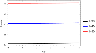
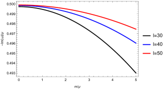
Figure 9: The behaviour of $Re(\omega)/\mu$ (left panel), and $-Im(\omega)/\mu$ (right panel) as a function of $m/\mu$ for different values of $\ell$ using the six order WKB method and $n=0$.

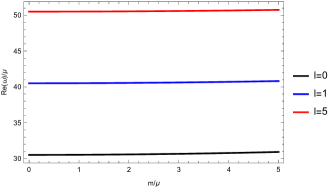
Figure 10: The behaviour of $Re(\omega)/\mu$ (left panel), and $-Im(\omega)/\mu$ (right panel) as a function of $m/\mu$ for different values of $\ell$ using the six order WKB method and $n=1$.

VI Conclusions

In this work, we explored generalized Bronnikov-Ellis wormholes as background geometries and investigated the propagation of massive scalar fields. The first wormhole spacetime arises as a solution to an action comprising the pure Einstein-Hilbert term and a scalar field with negative kinetic energy. The second wormhole spacetime, on the other hand, results from $f(R)$-gravity.

For the first wormhole spacetime, our analysis focused primarily on low values of the angular number $\ell$, and we determined the QNFs using the CFM. These QNFs exhibit an inverted behaviour of $Im(\omega)b_{0}$: when $mb_{0}>m_{c}b_{0}$, $Im(\omega)b_{0}$ increases with $\ell$, representing an anomalous decay rate of the QNMs. Conversely, for $mb_{0}<m_{c}b_{0}$, $Im(\omega)b_{0}$ decreases with increasing $\ell$ for $n\geq\ell$. The critical value $m_{c}b_{0}$ rises with an increase in the parameter $M/b_{0}$, and the frequency of the oscillation increases with both the angular number and the parameter $mb_{0}$. Additionally, we identified bound states characterized by an oscillation frequency without decay that rises with increasing $mb_{0}$ and $\ell$.

For the second wormhole spacetime, we obtained exact results for the QNFs, which, for large values of $\ell$, coincide with the third-order WKB approximation. Here, the longest-lived modes are those with the lowest angular number $\ell$, both for the fundamental and the first overtone. Furthermore, the oscillation frequency increases with a rise in the parameter $m/\mu$ and angular momentum $\ell$. Thus, in this wormhole background, the anomalous behaviour observed in the first spacetime is avoided. Also, the effective potential is symmetric about the throat of the wormhole and it does not allow wells, consequently bound states are not supported in this wormhole spacetime.

Acknowlegements

This work is partially supported by ANID Chile through FONDECYT Grant Nº 1220871 (P.A.G., and Y. V.).

Appendix A Numerical values

In this appendix we provide some numerical values of the QNFs via CFM for the generalized Bronnikov-Ellis wormholes. In Table 2 and 3 we show the QNFs for the fundamental mode for $M/b_{0}=0.1$, and $M/b_{0}=0.25$, respectively, and in Table 4 and 5 we show the QNFs for the first overtone ($n=1$) for $M/b_{0}=0.1$, and $M/b_{0}=0.25$, respectively.

Table 2: Fundamental $n=0$ QNFs $\omega b_{0}$ for scalar perturbations for the generalized Bronnikov-Ellis wormhole with $M/b_{0}=0.1$, for several values of the angular momentum and the mass of the scalar field using the CFM.

$\ell$	$mb_{0}=0$	$mb_{0}=0.2$	$mb_{0}=0.4$	$mb_{0}=0.6$
0	0.64217472 - 0.52979187 i	0.65556756 - 0.51733481 i	0.69692010 - 0.48206571 i	0.76830083 - 0.43049763 i
1	1.42443104 - 0.44987061 i	1.43440781 - 0.44629804 i	1.46408863 - 0.43594442 i	1.51272479 - 0.41981413 i
2	2.28995771 - 0.43248900 i	2.29664353 - 0.43105279 i	2.31660278 - 0.42681157 i	2.34954643 - 0.41995908 i
3	3.17040105 - 0.42628276 i	3.17533511 - 0.42552688 i	3.19009512 - 0.42327874 i	3.21455621 - 0.41959546 i
5	4.94550683 - 0.42182228 i	4.94871268 - 0.42151025 i	4.95831818 - 0.42057757 i	4.97428747 - 0.41903441 i
10	9.40544221 - 0.41934024 i	9.40713911 - 0.41925382 i	9.41222797 - 0.41899482 i	9.42070336 - 0.41856403 i
15	13.87311667 - 0.41879955 i	13.87426865 - 0.41875982 i	13.87772405 - 0.41864067 i	13.88348113 - 0.41844227 i
$\ell$	$mb_{0}=0.8$	$mb_{0}=1.0$	$mb_{0}=1.2$	$mb_{0}=1.4$
0	0.86912831 - 0.37246044 i	0.99422781 - 0.31703053 i	1.13627138 - 0.26904009 i	1.28910794 - 0.22942901 i
1	1.57908796 - 0.39932068 i	1.66154662 - 0.37599623 i	1.75820800 - 0.35123892 i	1.86709221 - 0.32616103 i
2	2.39501097 - 0.41079193 i	2.45238427 - 0.39967609 i	2.52093849 - 0.38701017 i	2.59986671 - 0.37319156 i
3	3.24851550 - 0.41456774 i	3.29169959 - 0.40831378 i	3.34377421- 0.40097186 i	3.40435536 - 0.39269243 i
5	4.99656144 - 0.41689732 i	5.02505886 - 0.41418882 i	5.05967769 - 0.41093663 i	5.10029687 - 0.40717299 i
10	9.43255622 - 0.41796278 i	9.44777395 - 0.41719290 i	9.46634048 - 0.41625671 i	9.48823630 - 0.41515702 i
15	13.89153706 - 0.41816492 i	13.90188784 - 0.41780899 i	13.91452839 - 0.41737499 i	13.92945250 - 0.41686353 i

Table 3: Fundamental $n=0$ QNFs $\omega b_{0}$ for scalar perturbations for the generalized Bronnikov-Ellis wormhole with $M/b_{0}=0.25$, for several values of the angular momentum and the mass of the scalar field using the CFM.

$\ell$	$mb_{0}=0$	$mb_{0}=0.2$	$mb_{0}=0.4$	$mb_{0}=0.6$
0	0.57954862 - 0.38454705 i	0.58788305 - 0.37466006 i	0.61338274 - 0.34648046 i	0.65699718 - 0.30486477 i
1	1.17377910 - 0.30720290 i	1.18130424 - 0.30383997 i	1.20370378 - 0.29401135 i	1.24044319 - 0.27843471 i
2	1.84793711 - 0.28302527 i	1.85314787 -0.28162482 i	1.86870696 - 0.27747445 i	1.89439869 - 0.27072045 i
3	2.53780145 - 0.27199629 i	2.54168130 - 0.27124742 i	2.55328871 - 0.26901575 i	2.57252849 - 0.26534505 i
5	3.93343488 - 0.26196975 i	3.93596757 - 0.26165516 i	3.94355629 - 0.26071402 i	3.95617323 - 0.25915412 i
10	7.45015539 - 0.25438498 i	7.45149755 - 0.25429618 i	7.45552258 - 0.25402996 i	7.46222623 - 0.25358694 i
15	10.97800980 - 0.25223172 i	10.97892087 - 0.25219058 i	10.98165362 - 0.25206720 i	10.98620671 - 0.25186172 i
$\ell$	$mb_{0}=0.8$	$mb_{0}=1.0$	$mb_{0}=1.2$	$mb_{0}=1.4$
0	0.71935825 - 0.25784028 i	0.80016054 - 0.21267941 i	0.89645704 - 0.17253589 i	1.00377455 - 0.13801622 i
1	1.29062276 - 0.25811736 i	1.35299556 - 0.23413835 i	1.42601082 - 0.20745244 i	1.50784347 - 0.17879248 i
2	1.92987630 - 0.26158567 i	1.97468010 - 0.25034262 i	2.02826070 - 0.23728299 i	2.09000500 - 0.22268827 i
3	2.59924592 - 0.26030455 i	2.63323242 - 0.25398401 i	2.67423284 - 0.24648753 i	2.72195391 - 0.23792684 i
5	3.97377260 - 0.25698816 i	3.99629142 - 0.25423331 i	4.02365065 - 0.25091069 i	4.05575648 - 0.24704466 i
10	7.47160139 - 0.25296810 i	7.48363819 - 0.25217484 i	7.49832401 - 0.25120891 i	7.51564357 - 0.25007240 i
15	10.99257790 - 0.25157433 i	11.00076404 - 0.25120533 i	11.01076114 - 0.25075510 i	11.02256429 - 0.25022409 i

Table 4: First overtone $n=1$ QNFs $\omega b_{0}$ for scalar perturbations for the generalized Bronnikov-Ellis wormhole with $M/b_{0}=0.1$, for several values of the angular momentum and the mass of the scalar field using the CFM.

$\ell$	$mb_{0}=0$	$mb_{0}=0.2$	$mb_{0}=0.4$	$mb_{0}=0.6$
0	0.48215901 - 1.83934960 i	0.48355134 - 1.83211141 i	0.48784214 - 1.81024999 i	0.49539239 - 1.77331563 i
1	1.18531283 - 1.43535637 i	1.18973778 - 1.42849651 i	1.20321550 - 1.40798383 i	1.22635308 - 1.37404779 i
2	2.13978782 - 1.32436578 i	2.14484682 - 1.32066795 i	2.16004435 - 1.30966487 i	2.18543533 - 1.29162649 i
3	3.06406448 - 1.29198825 i	3.06835811 - 1.28988826 i	3.08122789 - 1.28362767 i	3.10263958 - 1.27332322 i
5	4.87885201 - 1.27072447 i	4.88188492 - 1.26981683 i	4.89097566 - 1.26710268 i	4.90610018 - 1.26260811 i
10	9.37098143 - 1.25947857 i	9.37265290 - 1.25922149 i	9.37766566 - 1.25845099 i	9.38601480 - 1.25716938 i
15	13.84985433 - 1.25707137 i	13.85099838 - 1.25695263 i	13.85442998 - 1.25659656 i	13.86014749 - 1.25600367 i
$\ell$	$mb_{0}=0.8$	$mb_{0}=1.0$	$mb_{0}=1.2$	$mb_{0}=1.4$
0	0.50687537 - 1.72052831 i	0.52341091 - 1.65073531 i	0.54681941 - 1.56236912 i	0.58009574 - 1.45346680 i
1	1.26014835 - 1.32716772 i	1.30593642 - 1.26821760 i	1.36524947 - 1.19864836 i	1.43954101 - 1.12064318 i
2	2.22108946 - 1.26699755 i	2.26706119 - 1.23638676 i	2.32335302 - 1.20054689 i	2.38987830 - 1.16034332 i
3	3.13253313 - 1.25916454 i	3.17081881 - 1.24140704 i	3.21737287 - 1.22036208 i	3.27203347 - 1.19638504 i
5	4.92721862 - 1.25637588 i	4.60133237 - 2.98594631 i	4.62635318 - 2.96656927 i	5.02590622 - 1.22790668 i
10	9.39769212 - 1.25538044 i	9.41268624 - 1.25308945 i	9.43098258 - 1.25030310 i	9.45256345 - 1.24702947 i
15	13.86814819 - 1.25517478 i	13.87842828 - 1.25411105 i	13.89098288 - 1.25281395 i	13.90580606 - 1.25128527 i

Table 5: First overtone $n=1$ QNFs $\omega b_{0}$ for scalar perturbations for the generalized Bronnikov-Ellis wormhole with $M/b_{0}=0.25$, for several values of the angular momentum and the mass of the scalar field using the CFM.

$\ell$	$mb_{0}=0$	$mb_{0}=0.2$	$mb_{0}=0.4$	$mb_{0}=0.6$
0	0.58217648 - 1.31200598 i	0.58178419 - 1.30705341 i	0.58074738 - 1.29211492 i	0.57947867 - 1.26692340 i
1	1.10576623 - 0.99897774 i	1.10818210 - 0.99270181 i	1.11554218 - 0.97388846 i	1.12818333 - 0.94260457 i
2	1.82380452 - 0.88934468 i	1.82753835 - 0.88579921 i	1.83876095 - 0.87522321 i	1.85753019 - 0.85779732 i
3	2.53427660 - 0.84472565 i	2.53759327 - 0.84267946 i	2.54753715 - 0.83656988 i	2.56408904 - 0.82648272 i
5	3.94453789 - 0.80453084 i	3.94692945 - 0.80363037 i	3.95409834 - 0.80093568 i	3.96602715 - 0.79646673 i
10	7.46522687 - 0.77201761 i	7.46655166 - 0.77175658 i	7.47052476 - 0.77097406 i	7.47714240 - 0.76967182 i
15	10.99099654 - 0.76178973 i	10.99190286 - 0.76166781 i	10.99462141 - 0.76130218 i	10.99915090 - 0.76069321 i
$\ell$	$mb_{0}=0.8$	$mb_{0}=1.0$	$mb_{0}=1.2$	$mb_{0}=1.4$
0	0.57864581 - 1.23096746 i	0.57916915 - 1.18343640 i	0.58228934 - 1.12319399 i	0.58978003 - 1.04879086 i
1	1.14666028 - 0.89904448 i	1.17171924 - 0.84366508 i	1.20422868 - 0.77738301 i	1.24504510 - 0.70180079 i
2	1.88392504 - 0.83381987 i	1.91802066 - 0.80370035 i	1.95985689 - 0.76794601 i	2.00940382 - 0.72713929 i
3	2.58721432- 0.81255726 i	2.61685953 - 0.79498064 i	2.65294831 - 0.77398025 i	2.69537748 - 0.74981414 i
5	3.98268698 - 0.79025619 i	4.00403759 - 0.78234861 i	4.03002761 - 0.77279927 i	4.06059492 - 0.76167277 i
10	7.48639830 - 0.76785275 i	7.49828374 - 0.76552089 i	7.51278752 - 0.76268135 i	7.52989613 - 0.75934031 i
15	11.00548923 - 0.75984153 i	11.01363344 - 0.75874802	11.02357975 - 0.75741379 i	11.03532354 - 0.75584020 i

Appendix B Comparison of CFM and WKB method

In Table 6 we show the fundamental QNFs and the first overtone calculated using the CFM and the WKB approximation, and we see a good agreement for high $\ell$. We show the relative error of the real and imaginary parts of the values obtained with the WKB method with respect to the values obtained with the CFM, which is defined by

$$\epsilon_{Re(\omega)} = \frac{\mid Re(\omega_{WKB})-Re(\omega_{CFM})\mid}{\mid Re(\omega_{CFM})\mid}\cdot 100\%\,,$$ (55)

$$\epsilon_{Im(\omega)} = \frac{\mid Im(\omega_{WKB})-Im(\omega_{CFM})\mid}{\mid Im(\omega_{CFM})\mid}\cdot 100\%\,,$$ (56)

where $\omega_{WKB}$ corresponds to the result obtained with the six-order WKB method, and $\omega_{CFM}$ denotes the result with the CFM. We can observe that the error does not exceed $\approx$ 22.5 $\%$ in the imaginary part, and $\approx$ 4.6 $\%$ in the real part, for low values of $\ell$. However, for high values of $\ell$ ($\ell=10,15$), the error does not exceed 0.0007 $\%$ in the imaginary part, and 3.60 $\cdot 10^{-5}\,\%$ in the real part. Also, as it was observed, the frequencies all have a negative imaginary part, which means that the propagation of massive scalar fields is stable in this background.

Table 6: QNFs $\omega b_{0}$ for massive scalar field perturbations $m=0.5$ for the generalized Bronnikov-Ellis wormhole with $M/b_{0}=0.1$, $n=0,1$, for several values of the angular momentum $\ell$ of the scalar field using the CFM and the six-order WKB approximation.

$n=0$
$\ell$	CFM	WKB	$\epsilon_{Re(\tilde{\omega})}(\%)$	$\epsilon_{Im(\tilde{\omega})}(\%)$
0	0.72878751 - 0.45774669 i	0.76209632 - 0.35470112 i	4.5704	22.5115
1	1.48610337 - 0.42851924 i	1.50406001 - 0.41070253 i	1.2083	4.1577
2	2.33147670 - 0.42369524 i	2.33358638 - 0.42204168 i	0.0905	0.3903
3	3.20112396 - 0.42161155 i	3.20146777 - 0.42132985 i	0.0107	0.0668
5	4.96551051 - 0.41988141 i	4.96553585 - 0.41985314 i	0.0005	0.0067
10	9.41604283 - 0.41880083 i	9.41604328 - 0.41879991 i	$4.78\cdot 10^{-6}$	0.0002
15	13.88031503 - 0.41855136 i	13.88031506 - 0.41855126 i	$2.16\cdot 10^{-7}$	$2.39\cdot 10^{-5}$
$n=1$
$\ell$	CFM	WKB	$\epsilon_{Re(\tilde{\omega})}(\%)$	$\epsilon_{Im(\tilde{\omega})}(\%)$
0	0.49117622 - 1.79370750 i	0.41768809 - 1.55508806 i	14.9617	13.3031
1	1.21352327 - 1.39267106 i	1.24154163 - 1.26985185 i	2.3088	8.8190
2	2.17146134 - 1.30150131 i	2.18112283 - 1.28436587 i	0.4449	1.3166
3	3.09086911 - 1.27897071 i	3.09292339 - 1.27587774 i	0.0665	0.2418
5	4.89778582 - 1.26507565 i	4.89796016 - 1.26478685 i	0.0036	0.0228
10	9.38142361 - 1.25787387 i	9.38142698 - 1.25786520 i	$3.60\cdot 10^{-5}$	0.0007
15	13.85700314 - 1.25632967 i	13.85700340 - 1.25632873 i	$1.88\cdot 10^{-6}$	$7.48\cdot 10^{-5}$

References

- (1) L. Flamm, Phys. Z.17(1916) 448.
- (2) A. Einstein and N. Rosen, Phys. Rev.48(1935) 73.
- (3) C. W. Misner and J. A. Wheeler, Ann. Phys.2, 525 (1957); C. W. Misner, Phys. Rev.118, 1110 (1960).
- (4) J. A. Wheeler, Ann. Phys.2, 604 (1957);J. A. Wheeler, Geometrodynamics (Academic, New York, 1962).
- (5) K. A. Bronnikov, “Scalar-tensor theory and scalar charge,” Acta Phys. Polon. B 4, 251-266 (1973)
- (6) H. G. Ellis, “Ether flow through a drainhole - a particle model in general relativity,” J. Math. Phys. 14, 104-118 (1973)
- (7) M.S. Morris and K.S. Thorne, Am. J. Phys.56, 395 (1988); M. S. Morris, K. S. Thorne and U. Yurtsever,Phys. Rev. Lett.61, 1446 (1988).
- (8) V. Sahni and A. A. Starobinsky, Int. J. Mod. Phys. D09, 373 (2000); S. M. Carroll, Living Rev. Rel.4, 1 (2001); P. J. E. Peebles and B. Ratra, Rev. Mod. Phys.75, 559 (2003); P. F. Gonzales-Diaz, Phys. Rev. D65, 104035 (2002).
- (9) E. Poisson and M. Visser, “Thin shell wormholes: Linearization stability,” Phys. Rev. D 52, 7318-7321 (1995) [arXiv:gr-qc/9506083 [gr-qc]].
- (10) Y. Fujii, K. Maeda, ”The scalar-tensor theory of gravitation” (Cambridge University Press, 2007).
- (11) G. W. Horndeski, “Second-order scalar-tensor field equations in a four-dimensional space,” Int. J. Theor. Phys. 10, 363-384 (1974)
- (12) T. Kolyvaris, G. Koutsoumbas, E. Papantonopoulos, G. Siopsis, Scalar Hair from a Derivative Coupling of a Scalar Field to the Einstein Tensor. Class. Quant. Grav. 29, 205011 (2012)
- (13) M. Rinaldi, “Black holes with non-minimal derivative coupling,” Phys. Rev. D 86, 084048 (2012) [arXiv:1208.0103 [gr-qc]].
- (14) T. Kolyvaris, G. Koutsoumbas, E. Papantonopoulos and G. Siopsis, “Phase Transition to a Hairy Black Hole in Asymptotically Flat Spacetime,” JHEP 11, 133 (2013) [arXiv:1308.5280 [hep-th]].
- (15) E. Babichev and C. Charmousis, “Dressing a black hole with a time-dependent Galileon,” JHEP 08, 106 (2014) [arXiv:1312.3204 [gr-qc]].
- (16) C. Charmousis, T. Kolyvaris, E. Papantonopoulos and M. Tsoukalas, “Black Holes in Bi-scalar Extensions of Horndeski Theories,” JHEP 07, 085 (2014) [arXiv:1404.1024 [gr-qc]].
- (17) R. V. Korolev and S. V. Sushkov, “Exact wormhole solutions with nonminimal kinetic coupling,” Phys. Rev. D 90, 124025 (2014) [arXiv:1408.1235 [gr-qc]].
- (18) R. Korolev, F. S. N. Lobo and S. V. Sushkov, “General constraints on Horndeski wormhole throats,” Phys. Rev. D 101, no.12, 124057 (2020) [arXiv:2004.12382 [gr-qc]].
- (19) R. Korolev, F. S. N. Lobo and S. V. Sushkov, “Kinetic gravity braiding wormhole geometries,” [arXiv:2009.04829 [gr-qc]].
- (20) G. Koutsoumbas, I. Mitsoulas and E. Papantonopoulos, “Quantum Effects in Galileon Black Holes,” Class. Quant. Grav. 35, no.23, 235016 (2018) [arXiv:1803.05489 [gr-qc]].
- (21) N. Chatzifotis, G. Koutsoumbas and E. Papantonopoulos, “Formation of bound states of scalar fields in AdS-asymptotic wormholes,” Phys. Rev. D 104, no.2, 024039 (2021) [arXiv:2011.08770 [gr-qc]].
- (22) LIGO Scientific and Virgo Collaborations collaboration, B. P. Abbott et al., Observation of Gravitational Waves from a Binary Black Hole Merger, Phys. Rev. Lett. 116 (2016) 061102.
- (23) VGW151226: Observation of Gravitational Waves from a 22-Solar-Mass Binary Black Hole Coalescence, Phys. Rev. Lett. 116 (2016) 241103.
- (24) VIRGO, LIGO Scientific collaboration, B. P. Abbott et al., GW170104: Observation of a 50-Solar-Mass Binary Black Hole Coalescence at Redshift 0.2, Phys. Rev. Lett. 118 (2017) 221101.
- (25) Virgo, LIGO Scientific collaboration, B. P. Abbott et al., GW170814: A Three-Detector Observation of Gravitational Waves from a Binary Black Hole Coalescence, Phys. Rev. Lett. 119 (2017) 141101.
- (26) Virgo, LIGO Scientific collaboration, B. P. Abbott et al., GW170817: Observation of Gravitational Waves from a Binary Neutron Star Inspiral, Phys. Rev. Lett. 119 (2017) 161101.
- (27) C. V. Vishveshwara, “Scattering of Gravitational Radiation by a Schwarzschild Black-hole,” Nature 227, 936 (1970).
- (28) K. D. Kokkotas and B. G. Schmidt, “Quasinormal modes of stars and black holes,” Living Rev. Rel. 2, 2 (1999) [gr-qc/9909058].
- (29) E. Berti, V. Cardoso and A. O. Starinets, “Quasinormal modes of black holes and black branes,” Class. Quant. Grav. 26, 163001 (2009) [arXiv:0905.2975 [gr-qc]].
- (30) P. O. Mazur and E. Mottola, “Gravitational condensate stars: An alternative to black holes,” [arXiv:gr-qc/0109035 [gr-qc]].
- (31) M. S. Morris, K. S. Thorne and U. Yurtsever, “Wormholes, Time Machines, and the Weak Energy Condition,” Phys. Rev. Lett. 61, 1446-1449 (1988)
- (32) T. Damour and S. N. Solodukhin, “Wormholes as black hole foils,” Phys. Rev. D 76, 024016 (2007) [arXiv:0704.2667 [gr-qc]].
- (33) R. A. Konoplya and A. Zhidenko, “Quasinormal modes of black holes: From astrophysics to string theory,” Rev. Mod. Phys. 83 (2011), 793-836 [arXiv:1102.4014 [gr-qc]].
- (34) V. Cardoso, E. Franzin and P. Pani, “Is the gravitational-wave ringdown a probe of the event horizon?,” Phys. Rev. Lett. 116 (2016) no.17, 171101 [arXiv:1602.07309 [gr-qc]].
- (35) P. O. Mazur and E. Mottola, “Gravitational condensate stars: An alternative to black holes,” [arXiv:gr-qc/0109035 [gr-qc]].
- (36) T. Damour and S. N. Solodukhin, “Wormholes as black hole foils,” Phys. Rev. D 76, 024016 (2007) [arXiv:0704.2667 [gr-qc]].
- (37) B. Holdom and J. Ren, “Not quite a black hole,” Phys. Rev. D 95, no.8, 084034 (2017) [arXiv:1612.04889 [gr-qc]].
- (38) K. D. Kokkotas and B. G. Schmidt, “Quasinormal modes of stars and black holes,” Living Rev. Rel. 2, 2 (1999) [gr-qc/9909058].
- (39) E. Berti, V. Cardoso and A. O. Starinets, “Quasinormal modes of black holes and black branes,” Class. Quant. Grav. 26, 163001 (2009) [arXiv:0905.2975 [gr-qc]].
- (40) R. A. Konoplya and A. V. Zhidenko, “Decay of massive scalar field in a Schwarzschild background,” Phys. Lett. B 609 (2005), 377-384 [arXiv:gr-qc/0411059 [gr-qc]].
- (41) R. A. Konoplya and A. Zhidenko, “Stability and quasinormal modes of the massive scalar field around Kerr black holes,” Phys. Rev. D 73 (2006), 124040 [arXiv:gr-qc/0605013 [gr-qc]].
- (42) S. R. Dolan, “Instability of the massive Klein-Gordon field on the Kerr spacetime,” Phys. Rev. D 76, 084001 (2007) [arXiv:0705.2880 [gr-qc]].
- (43) O. J. Tattersall and P. G. Ferreira, “Quasinormal modes of black holes in Horndeski gravity,” Phys. Rev. D 97, no. 10, 104047 (2018) [arXiv:1804.08950 [gr-qc]].
- (44) A. Aragón, P. A. González, E. Papantonopoulos and Y. Vásquez, “Anomalous decay rate of quasinormal modes in Schwarzschild-dS and Schwarzschild-AdS black holes,” JHEP 08 (2020), 120 [arXiv:2004.09386 [gr-qc]].
- (45) R. D. B. Fontana, P. A. González, E. Papantonopoulos and Y. Vásquez, “Anomalous decay rate of quasinormal modes in Reissner-Nordström black holes,” Phys. Rev. D 103, no.6, 064005 (2021) [arXiv:2011.10620 [gr-qc]].
- (46) P. A. González, E. Papantonopoulos, J. Saavedra and Y. Vásquez, “Quasinormal modes for massive charged scalar fields in Reissner-Nordström dS black holes: anomalous decay rate,” JHEP 06 (2022), 150 [arXiv:2204.01570 [gr-qc]].
- (47) A. Aragón, R. Bécar, P. A. González and Y. Vásquez, “Massive Dirac quasinormal modes in Schwarzschild–de Sitter black holes: Anomalous decay rate and fine structure,” Phys. Rev. D 103 (2021) no.6, 064006 [arXiv:2009.09436 [gr-qc]].
- (48) K. Destounis, R. D. B. Fontana and F. C. Mena, “Accelerating black holes: quasinormal modes and late-time tails,” Phys. Rev. D 102 (2020) no.4, 044005 [arXiv:2005.03028 [gr-qc]].
- (49) A. Aragón, P. A. González, E. Papantonopoulos and Y. Vásquez, “Quasinormal modes and their anomalous behavior for black holes in gravity,” Eur. Phys. J. C 81 (2021) no.5, 407 [arXiv:2005.11179 [gr-qc]].
- (50) A. Aragón, P. A. González, J. Saavedra and Y. Vásquez, “Scalar quasinormal modes for -dimensional Coulomb-like AdS black holes from nonlinear electrodynamics,” Gen. Rel. Grav. 53 (2021) no.10, 91 [arXiv:2104.08603 [gr-qc]].
- (51) R. A. Konoplya and C. Molina, “The Ringing wormholes,” Phys. Rev. D 71 (2005), 124009 [arXiv:gr-qc/0504139 [gr-qc]].
- (52) R. A. Konoplya and A. Zhidenko, “Wormholes versus black holes: quasinormal ringing at early and late times,” JCAP 12, 043 (2016) [arXiv:1606.00517 [gr-qc]].
- (53) M. S. Churilova, R. A. Konoplya and A. Zhidenko, “Arbitrarily long-lived quasinormal modes in a wormhole background,” Phys. Lett. B 802 (2020), 135207 [arXiv:1911.05246 [gr-qc]].
- (54) R. A. Konoplya, “How to tell the shape of a wormhole by its quasinormal modes,” Phys. Lett. B 784 (2018), 43-49 [arXiv:1805.04718 [gr-qc]].
- (55) J. L. Blázquez-Salcedo, X. Y. Chew and J. Kunz, “Scalar and axial quasinormal modes of massive static phantom wormholes,” Phys. Rev. D 98, no.4, 044035 (2018) [arXiv:1806.03282 [gr-qc]].
- (56) P. A. González, E. Papantonopoulos, Á. Rincón and Y. Vásquez, “Quasinormal modes of massive scalar fields in four-dimensional wormholes: Anomalous decay rate,” Phys. Rev. D 106, no.2, 024050 (2022) [arXiv:2205.06079 [gr-qc]].
- (57) B. Azad, J. L. Blázquez-Salcedo, X. Y. Chew, J. Kunz and D. h. Yeom, Phys. Rev. D 107, no.8, 084024 (2023) [arXiv:2212.12601 [gr-qc]].
- (58) T. Karakasis, E. Papantonopoulos, Z. Y. Tang and B. Wang, Phys. Rev. D 103, no.6, 064063 (2021) doi:10.1103/PhysRevD.103.064063 [arXiv:2101.06410 [gr-qc]].
- (59) T. Karakasis, E. Papantonopoulos, Z. Y. Tang and B. Wang, Eur. Phys. J. C 81, no.10, 897 (2021) [arXiv:2103.14141 [gr-qc]].
- (60) Z. Y. Tang, B. Wang and E. Papantonopoulos, Eur. Phys. J. C 81, no.4, 346 (2021) [arXiv:1911.06988 [gr-qc]].
- (61) T. Karakasis, E. Papantonopoulos and C. Vlachos, “f(R) gravity wormholes sourced by a phantom scalar field,” Phys. Rev. D 105, no.2, 024006 (2022) [arXiv:2107.09713 [gr-qc]].
- (62) K. A. Bronnikov, Particles 1, no.1, 56-81 (2018) [arXiv:1802.00098 [gr-qc]].
- (63) G. C. Samanta and N. Godani, Eur. Phys. J. C 79, no.7, 623 (2019) [arXiv:1908.04406 [gr-qc]].
- (64) C. Muller, in Lecture Notes in Mathematics: Spherical Harmonics Springer-Verlag, Berlin-Heidelberg, 1966.
- (65) E. W. Leaver, “An Analytic representation for the quasi normal modes of Kerr black holes,” Proc. Roy. Soc. Lond. A 402, 285-298 (1985)
- (66) E. W. Leaver, “Quasinormal modes of Reissner-Nordstrom black holes,” Phys. Rev. D 41, 2986-2997 (1990)
- (67) H. P. Nollert, “Quasinormal modes of Schwarzschild black holes: The determination of quasinormal frequencies with very large imaginary parts,” Phys. Rev. D 47, 5253-5258 (1993)
- (68) V. Cardoso, J. P. S. Lemos and S. Yoshida, JHEP 12, 041 (2003) [arXiv:hep-th/0311260 [hep-th]].
- (69) R. A. Konoplya and A. Zhidenko, “Massive charged scalar field in the Kerr-Newman background I: quasinormal modes, late-time tails and stability,” Phys. Rev. D 88, 024054 (2013) [arXiv:1307.1812 [gr-qc]].
- (70) M. Richartz and D. Giugno, “Quasinormal modes of charged fields around a Reissner-Nordström black hole,” Phys. Rev. D 90, no.12, 124011 (2014) [arXiv:1409.7440 [gr-qc]].
- (71) A. Chowdhury and N. Banerjee, “Quasinormal modes of a charged spherical black hole with scalar hair for scalar and Dirac perturbations,” Eur. Phys. J. C 78, no.7, 594 (2018) [arXiv:1807.09559 [gr-qc]].
- (72) R. Bécar, P. A. González and Y. Vásquez, “Quasinormal modes of a charged scalar field in Ernst black holes,” Eur. Phys. J. C 83, no.1, 75 (2023) [arXiv:2211.02931 [gr-qc]].
- (73) K. A. Bronnikov, R. A. Konoplya and T. D. Pappas, “General parametrization of wormhole spacetimes and its application to shadows and quasinormal modes,” Phys. Rev. D 103, no.12, 124062 (2021) [arXiv:2102.10679 [gr-qc]].
- (74) S. Aneesh, S. Bose and S. Kar, “Gravitational waves from quasinormal modes of a class of Lorentzian wormholes,” Phys. Rev. D 97, no.12, 124004 (2018) [arXiv:1803.10204 [gr-qc]].
- (75) P. Dutta Roy, S. Aneesh and S. Kar, “Revisiting a family of wormholes: geometry, matter, scalar quasinormal modes and echoes,” Eur. Phys. J. C 80, no.9, 850 (2020) [arXiv:1910.08746 [gr-qc]].
- (76) B. Mashhoon, “Quasi-normal modes of a black hole,” Third Marcel Grossmann Meeting on General Relativity 1983.
- (77) B. F. Schutz and C. M. Will, “BLACK HOLE NORMAL MODES: A SEMIANALYTIC APPROACH,” Astrophys. J. Lett. 291 (1985), L33-L36
- (78) S. Iyer and C. M. Will, “Black Hole Normal Modes: A WKB Approach. 1. Foundations and Application of a Higher Order WKB Analysis of Potential Barrier Scattering,” Phys. Rev. D 35 (1987), 3621
- (79) R. A. Konoplya, “Quasinormal behavior of the d-dimensional Schwarzschild black hole and higher order WKB approach,” Phys. Rev. D 68 (2003), 024018 [arXiv:gr-qc/0303052 [gr-qc]].
- (80) J. Matyjasek and M. Opala, “Quasinormal modes of black holes. The improved semianalytic approach,” Phys. Rev. D 96 (2017) no.2, 024011 [arXiv:1704.00361 [gr-qc]].
- (81) R. A. Konoplya, A. Zhidenko and A. F. Zinhailo, “Higher order WKB formula for quasinormal modes and grey-body factors: recipes for quick and accurate calculations,” Class. Quant. Grav. 36 (2019), 155002 [arXiv:1904.10333 [gr-qc]].
- (82) Y. Hatsuda, “Quasinormal modes of black holes and Borel summation,” Phys. Rev. D 101 (2020) no.2, 024008 [arXiv:1906.07232 [gr-qc]].