Classifier Surrogates: Sharing AI-based Searches with the World

Abstract

In recent years, neural network-based classification has been used to improve data analysis at collider experiments. While this strategy proves to be hugely successful, the underlying models are not commonly shared with the public and they rely on experiment-internal data as well as full detector simulations. We propose a new strategy, so-called classifier surrogates, to be trained inside the experiments, that only utilise publicly accessible features and truth information. These surrogates approximate the original classifier distribution, and can be shared with the public. Subsequently, such a model can be evaluated by sampling the classification output from high-level information without requiring a sophisticated detector simulation. Technically, we show that Continuous Normalizing Flows are a suitable generative architecture that can be efficiently trained to sample classification results using Conditional Flow Matching. We further demonstrate that these models can be easily extended by Bayesian uncertainties to indicate their degree of validity when confronted with unknown inputs to the user. For a concrete example of tagging jets from hadronically decaying top quarks, we demonstrate the application of flows in combination with uncertainty estimation through either inference of a mean-field Gaussian weight posterior, or Monte Carlo sampling network weights.

1 Introduction

Current experimental work in particle physics, for example by the ATLAS and CMS collaborations, uses deep-learning based taggers to great success [1, 2, 3, 4]. Such models often define unique and essential quantities in the analysis chain, which are hard to understand in terms of physical quantities. While the performance benefit is apparent, best practises for sharing the analysis as for traditional cut-based analyses [5, 6] are not yet established. This especially hinders the re-interpretation of experimental results. Recently, a first set of proposals on sharing neural-network based results has been published [7]. On the purely technical side, solutions exist for sharing serialized networks [8, 9] and some first searches shared with serialized models have been made public [10, 11, 12, 13].

However, when the model inputs contain features which are not available outside the collaborations, for example detector level quantities, such as hits, or highly detector dependent quantities, such as soft jet-substructure variables, the benefit of sharing the network weights is limited as results still cannot be reproduced. For example, both $b$-taggers of ATLAS and CMS use detector dependent information [14, 15] and current research shows the best classification performance is achieved when using detector level data, rather than only high-level observables [4, 16]. For these cases, sharing a surrogate model trained to reproduce the classification results from truth-, parton- or reconstruction-level inputs has recently been proposed [7]. We will refer to such models as Classifier Surrogates and in this work demonstrate for a concrete example how such a classifier could be constructed and evaluated.

Surrogates allow researchers from outside the collaboration to build on the results of the search by easily evaluating the sensitivity to other signatures or quickly estimating the analysis performance without performing the costly detector simulation, all independent of the researches affiliation. Limited information comes with a price in terms of increased uncertainty, and Classifier Surrogates also need to be able to correctly predict the loss in precision thus incurred.

In Section 3, we discuss why a Classifier Surrogate needs to employ a generative architecture and introduce two possible architectures in Section 4, including a novel combination of Continuous Normalizing Flows with Monte Carlo-based Bayesian deep learning. We employ the architecture to a toy example with a classifier derived from the Particle Transformer [16]. This setup is introduced in Section 2. In Section 5, we discuss the performance of the surrogate both for data within the distribution of the training data, as well as for data new to the model. We evaluate calibration and scaling to the tails of the distribution, as well as out-of-distribution indication.

2 Particle Transformer and JetClass Dataset

As internal taggers of the big collaborations are not available for public study, we use the state-of-the-art jet tagger, the Particle Transformer (ParT) [16]. ParT is an attention-based model trained to distinguish $10$ different types of jets using per-particle information and trained on the $100$M JetClass dataset [17]. The features include kinematics, particle identification, and trajectory displacement of every particle in the jet.

From the large initial JetClass dataset as stand-in for the internal collaboration datasets, we distill our dataset by calculating transverse momentum, pesudorapidity, scattering angle, jet energy, number of particles, soft drop mass [18] and N-subjettiness [19] for $N=1,...,4$ as well as the output of the full ParT for the regarding event. For the first studies we will restrain the experiments to the first five jet observables as well as the true top or QCD label.

While learning a surrogate of a multiclassifier is possible by using a generative architecture with a multidimensional output space, we restrict the setup to binary classification of top jets. The toy train and validation datasets contain $1$M jet events each from $Z$-events and hadronic decay of $t\bar{t}$. To reduce the $10$-dimensional ParT output to a binary classification result, we rescale

$$p_{\mathrm{t\rightarrow bqq^{\prime}}}=\frac{p_{\mathrm{t\rightarrow bqq^{\prime}}}^{\mathrm{ParT}}}{p_{\mathrm{t\rightarrow bqq^{\prime}}}^{\mathrm{ParT}}+p_{\mathrm{Z\rightarrow qq^{\prime}}}^{\mathrm{ParT}}}.$$ (1)

3 Detector Smearing Distribution

Due to the stochasticity of the detector simulation, jets with the same high-level observables can differ a lot on detector level. These jets will thus result in different ParT outputs defining the posterior distribution per set of high-level observables

$$p(\,\mathrm{ParT}\,|\,p_{T},\eta,\phi,E_{\mathrm{jet}},n_{\mathrm{const}},...\,).$$ (2)

Based on its physical origin, we will refer to this distribution as the Detector Smearing Distribution.

We can generate a first approximation of this distribution by generating a histogram of the ParT output for the closest points in $p_{T}$, $E_{\mathrm{jet}}$ and $n_{\mathrm{const}}$. In Figure 1 we show this histogram for the $1000$ nearest jet events in the training sample for two arbitrary jet events in the bulk of the transverse momentum distribution at $p_{t}\approx 530\mathrm{GeV}$. The imperfect ParT classification introduces an output distribution with tails for events indistinguishable from the high-level features. These tails will eventually be modelled by the generative architecture introduced in Section 4.

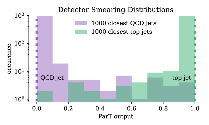
Figure 1: Histograms of the ParT classification results for the $1000$ jet events of the training data, closest to the two arbitrary jets indicated by the dotted lines. Although being classified with varying confidence from detector-level data, the high-level observables $p_{T}$, $E_{\mathrm{jet}}$ and $n_{\mathrm{const}}$ appear identical.

4 Bayesian Generative Architectures

To sample the distribution of the classification output conditioned on high-level jet features induced by detector smearing, we employ a conditional generative model. While all flavours of generative models have found multiple applications in high-energy physics, for example in [20] and [21], Normalizing Flows can easily and efficiently be applied to infer complex, low-dimensional conditional distributions [22, 23]. In our tests, coupling block-based Normalizing Flows exhibit great performance for dense phase space regions, but larger deviations when modelling tails of distributions. To boost the performance of model we employ Continuous Normalizing Flows (CNF), a generalization of coupling block Flows based on ordinary differential equations (ODE) introduced in Section 4.1.

To prevent the application of the surrogate on data not included in tagger and thus surrogate training, we employ Bayesian Deep Learning frameworks. Through modeling of (or sampling from) a posterior weight distribution, these methods give a large spread of predictions for data not included in the loss objective during training. Sections 4.3 and 4.4 introduce two different approaches to Bayesian Neural Networks employed in this paper.

4.1 Continuous Normalizing Flows and Conditional Flow Matching

First introduced in [24], CNFs define a transformation $\phi_{t}:[0,1]\times\mathds{R}^{d}\rightarrow\mathds{R}^{d}$ called flow dependent on a time variable $t$. The time variable is the continuous equivalent to the number of a coupling blocks in a coupling block-flow [25]. Instead of having multiple flow instances, the dependence of $\phi$ on $t$ is defined through the ODE

$$\frac{\mathrm{d}}{\mathrm{d}t}\phi_{t}(x)=v_{t}(\phi_{t}(x)),\quad\phi_{0}(x)=x,$$ (3)

by the time dependent vector-field $v_{t}\colon[0,1]\times\mathds{R}^{d}\rightarrow\mathds{R}^{d}$, which itself is approximated by a deep neural network $\tilde{v}_{t}(\cdot,\theta)\approx v_{t}$. While this network can be arbitrarily complex, we stick to fully-connected architectures due to the low dimensionality of the task. In our case, the flow transforms data from a Gaussian distribution $\mathcal{N}(0,1)$ for $t=0$ into ParT output at $t=1$. This choice sets the boundaries of the probability path $p_{t}\colon[0,1]\times\mathds{R}^{d}\rightarrow\mathds{R}_{>0}$ induced by the vector-field trough Equation (3) and

$$p_{t}(x)=p_{0}\left(\phi_{t}^{-1}(x)\right)\det\left(\frac{\partial\phi_{t}^{-1}(x)}{\partial x}\right).$$ (4)

A standard CNF is trained by solving the ODE Equation (3) in reverse and minimizing the negative $\log$-likelihood (NLL) of input data at $t=1$. The computation of this loss objective is expensive, especially for larger dimensional models.

Thus, the authors of [26] introduce the Conditional Flow Matching (CFM) objective

$$\mathcal{L}_{\mathrm{CFM}}(\theta)=\mathds{E}_{t,q(x_{1}),p_{t}(x|x_{1})}\left\|u_{t}(x|x_{1})-\tilde{v}_{t}(x;\theta))\right\|^{2}$$ (5)

It reduces the calculation of the optimization criterion to the calculation of a mean-squared error between the network output $\tilde{v}_{t}(x;\theta)$ and an analytical solution $u_{t}$ for sampled $t\sim\mathcal{U}(0,1)$, $x_{1}\sim q$ and $x\sim p_{t}(\cdot|x_{1})$. Here, $q$ is the probability distribution of the input data. A good choice of $u_{t}$ and corresponding $p_{t}$ is the a Gaussian conditional probability path with mean and variance changing linear in time (optimal transport) [26]. The CFM-loss (5) then reduces even further

$$\mathcal{L}_{\mathrm{CFM}}(\theta)=\mathds{E}_{t,q(x_{1}),p(x_{0})}\Big{\|} \left(x_{1}-\left(1-\sigma_{\mathrm{min}}\right)x_{0}\right)$$ (6)

$$-\tilde{v}_{t}(\sigma_{t}x_{0}+\mu_{t};\theta))\Big{\|}^{2},$$

where $\mu_{t}=tx_{1}$, $\sigma_{t}=1-(1-\sigma_{\mathrm{min}})t$, $p(x_{0})=\mathcal{N}(0,1)$ and $\sigma_{\mathrm{min}}$ a small parameter, that can be chosen to match the noise level of the training data.

4.2 Conditional Denstity Estimation

Following the coupling-block Flow based example of [23], we can approximate a conditional density

$$p_{t}(x|c)=p_{0}\left(\phi_{t}^{-1}(x,c)|c\right)\det\left(\frac{\partial\phi_{t}^{-1}(x,c)}{\partial x}\right),$$ (7)

where the noise distribution is independent of the condition $p_{0}(\cdot|c)=p_{0}(\cdot)$. We thus append the vector of conditions to every layer of the vector field model $\tilde{v}_{t}(x,c\,;\theta)$ to ensure estimation of the conditional density.

4.3 Mean-Field Gaussian Variational Inference (VIB)

To infer a Bayesian uncertainty on the network output, that is the epistemic uncertainty, we approximate the posterior distribution $p\left(\theta\mid x\right)$ of the weights of $\tilde{v}_{t}(x,\theta)$ by an uncorrelated Normal distribution $\tilde{p}(\theta)$ [27]. This approximation is usually inferred during optimization of the network, by minimizing the Kullback-Leibler divergence ($D_{\mathrm{KL}}$) between the posterior and its approximation

$$\mathcal{L}_{\mathrm{BBB}} =D_{\mathrm{KL}}\left[\,\tilde{p}(\theta),p\left(\theta|x_{1}\right)\right]$$ (8)

$$=-\int\mathrm{d}\theta\,\tilde{p}(\theta)\,\log p\left(x_{1}|\theta\right)$$

$$\quad\quad\quad+D_{\mathrm{KL}}\left[\,\tilde{p}(\theta),p(\theta)\right]+\text{ constant}.$$

Following the construction in [28], we bridge the gap between the CFM-loss (6) and the $\log$-liklihood of the data in (8) by introducing a factor $c$ that can be optimized to account for the difference

$$\mathcal{L}_{\mathrm{BBB-CFM}}=\mathds{E}_{\tilde{p}(x_{1})}\mathcal{L}_{\mathrm{CFM}}+cD_{\mathrm{KL}}\left[\,\tilde{p}(\theta),p(\theta)\right].$$ (9)

4.4 AdamMCMC

While the derivation of the loss (9) lacks theoretic backing, the small size of the classification surrogate problem allows us to directly sample the weight posterior distribution through Markov Chain Monte Carlo (MCMC). We initialize the chain with a network optimized using the CFM-loss objective (6) and solve the ODE (3) to determine the negative $\log$-likelihood $\mathcal{L}_{\mathrm{NLL}}$ of the data for every step of the MCMC from there on.

To ensure detailed balance we employ a Metropolis-Hastings (MH) correction with acceptance rate

$$\alpha=\frac{\exp\left(-\lambda\mathcal{L}_{\mathrm{NLL}}(\tau_{i})\right)q(\theta_{i}|\tau_{i})}{\exp\left(-\lambda\mathcal{L}_{\mathrm{NLL}}(\theta_{i})\right)q(\tau_{i}|\theta_{i})}$$ (10)

for all steps of the chain. Here, the parameter $\lambda$ gives the inverse temperature of the tempered posterior distribution sampled from. The proposed weights $\tau_{i}$ are drawn from a proposal distribution centered on a gradient-descent step

$$\tilde{\theta}_{i+1}=\mathrm{Adam}(\theta_{i},\mathcal{L}_{\mathrm{NLL}}(\theta_{i}))$$ (11)

calculated using the Adam algorithm [29]. We can use the momentum terms of the update to ensure high acceptance-rates by smearing the proposal distribution in the direction of the last update

$$\tau_{i}\sim q(\cdot|\theta_{i})=\mathcal{N}(\tilde{\theta}_{i+1},\sigma^{2}\mathrm{1}+(\tilde{\theta}_{i+1}-\theta_{i})(\tilde{\theta}_{i+1}-\theta_{i})^{\top}).$$ (12)

To efficiently run this algorithm, we evaluate the NLL on batches of data. For proofs on convergence and invariant distribution of this algorithm, we refer to [30].

5 Results

To learn the Detector Smearing Distribution from data, we set up a CNF with $3$ multi-layer perceptrons (MLPs) with $3$ layers of dimension $64$ and $\operatorname{ELU}$ activation. The condition and time variable $t$ are concatenated to every MLP input, totalling in $31617$ network parameters. Converting to a VIB as in [27], doubles the number of parameters. We train on a balanced set of $4$M jets in batches of $131072$ for $4000$ epochs using Adam [29] with a constant learning rate of $10^{-3}$. As loss objective, we use the CFM-loss as introduced in Equations (6) and (9) respectively. To achieve good coverage, we choose $c=100$ and $\lambda=50$ from a course grid search over multiple orders of magnitude.

We run the AdamMCMC chain for another $1000$ epochs with the learning rate reduced to $5\cdot 10^{-6}$ and $\sigma=0.05$. For the sampled posterior we always report the results from CFM optimization in solid lines and the uncertainty calculated as the $\min$-$\max$-envelope of $10$ drawings, where for the learned approximation (VIB) we give the mean and the $\min$-$\max$-envelope over $11$ sets of weights.

5.1 In-Distribution

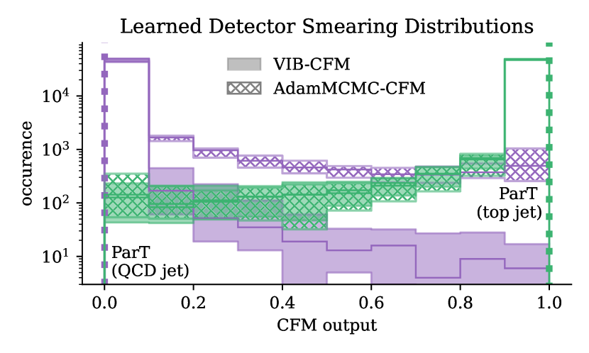
Figure 2: Histograms of $50000$ samples drawn form the Detector Smearing Distributions learned with a CFM model. Uncertainties are generated by drawing the samples from $11$ points sampled from the network posterior approximation or chain. The ParT-output for the arbitrary QCD and top jet used as condition is indicated with dotted lines. Both jet events are the same as for Figure 1.

We can use the trained CNFs to generate another approximation of the Detector Smearing Distribution by performing the forward direction starting at different points in latent space but for the same high-level features. Figure 2 shows histograms of the generated data for the same arbitrary jet events as Figure 1.

We can see similar distributions for the approximation with CNFs as for the histograms of the closest events. The biggest discrepancy occurs between the distribution for the arbitrary QCD jet obtained using AdamMCMC and VIB. It can be attributed to the difference between the model at initialization of the AdamMCMC chain and the posterior mean output of VIB. The initialization can be adapted to accommodate desired behaviours, if well defined, by choosing between different epochs of the CFM-optimization. Furthermore, increasing the chain length decreases the dependence of the ensemble output on the initialization overall.

5.1.1 Uncertainty Calibration

To find out whether predictions using AdamMCMC are in general conservative, we need to look at the calibration of the estimated Detector Smearing Distributions for multiple events, here $10000$. For every event, we calculate $q$-quantiles for 50 values of $q$ (nominal coverage) linearly spaced between $0$ and $1$. We then evaluate the empirical coverage, that is the fraction of events within their respective quantile. The calibration is perfect when nominal and empirical coverage agree. Figure 3 shows very good calibration for both methods, where AdamMCMC in fact tends to be slightly more confident than VIB approximations.

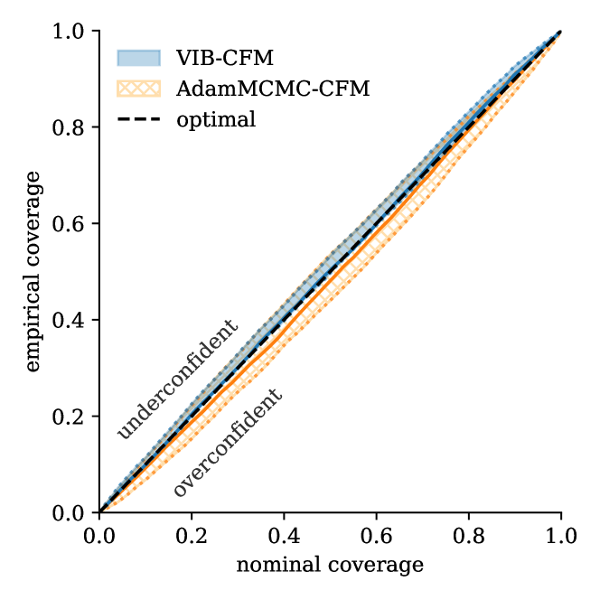
Figure 3: Empirical over nominal coverage calculated by taking $1000$ samples from the learned Detector Smearing Distribution for $10000$ jet events each. Uncertainties again are calculated from $11$ points of the network posterior.

5.1.2 Epistemic Uncertainty

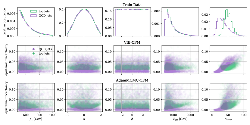
Figure 4: Epistemic uncertainty calculated from the mean difference between 11 points from the network posterior over $1000$ samples drawn from the respective learned Detector Smearing Distribution for each event of the validation set. The uncertainty shows a clear scaling towards the edges of the train data, as well es in regions where $n_{\mathrm{const}}$ is uninformative.

For a further dive into the behaviour of the epistemic uncertainty obtained from the posterior distribution of the network weights, we calculate the mean distance of the maximum discrepancy between instances of the network posterior

$$\delta_{\mathrm{epis}}=\frac{1}{n_{\mathrm{stat}}}\sum_{i=0}^{n_{\mathrm{stat}}}\left(\max_{\theta}\phi_{0,\theta}(x_{i})-\min_{\theta}\phi_{0,\theta}(x_{i})\right)$$ (13)

for a total of $n_{\mathrm{stat}}=1000$ points drawn from the Gaussian latent space $x_{1},...,x_{n_{\mathrm{stat}}}\sim\mathcal{N}(0,1)$. Ideally, this error estimate is large for sparsely populated areas of the high-level feature space and small in the bulk of the distribution. To investigate this behaviour, we plot a histogram of the high-level features of the training data as well as $\delta_{\mathrm{epis}}$ for $10000$ jet events chosen at random from a test set for both methods in Figure 4.

The most instructive panels show the dependence of the error estimate on the number of constituents in the jet $n_{\mathrm{const}}$, which is the most descriptive input feature. We can see high uncertainties occurring in the regions where the distributions for QCD and top jets overlap in the training data. These are events that can not easily be attributed to one of the two classes by the $5$ high-level observables alone, resulting in high uncertainties. These events also make up the high-error bulk when plotted over the other high-level features.

For every tailed distribution, we can also see an increase of the error estimate for top jet predictions towards the edges of the data. This behaviour is stronger for AdamMCMC than for VIB at the cost of higher uncertainties overall.

The same behaviour is not observed for QCD jets. This again can be traced back to the distribution of $n_{\mathrm{const}}$. Where the distribution of the number of particles of top jets is fully within the support of the one for QCD jets, it drops to zero for low numbers allowing a perfect classification of the QCD jets in this region.

5.1.3 Adding Informative Features

Another measure of the informative value of a Detector Smearing Distribution generated from the CNF is the predicted accuracy

predicted accuracy (14)

$$=\frac{1}{n_{\mathrm{stat}}}\sum_{i=0}^{n_{\mathrm{stat}}}\left\{\begin{array}[]{ll}\mathbf{1}_{[0.5,1]}\left(\phi_{0,\theta}(x_{i})\right)\text{ for a top jet}\\ \mathbf{1}_{[0,0.5)}\left(\phi_{0,\theta}(x_{i})\right)\text{ for a QCD jet}\\ \end{array}\right.$$

per jet event, with $\mathbf{1}_{A}(x)$ the indicator function of set $A$. The cut value of $0.5$ is arbitrary and can be chosen in line with the experimental analysis. Our choice reflects the requirement to yield symmetric output distributions in case of uninformative high-level input.

Figure 5 shows histograms of the predicted accuracy for $10000$ jet events chosen at random from the full balanced test set. It shows distributions generated from CNFs conditioned on the five high-level jet features introduced before, as well as for conditioning including the soft drop jet mass $m_{\mathrm{SD}}$ and the $N$-subjettiness for $N\in\{1,..,4\}$. Naively, we assume that adding more information will lead to more certain predictions and thus will shift the distributions towards high accuracy values. In the highest value bin, the information hierarchy is well reproduced, with the highest number of input features leading to the highest number of certain outputs. In the range of $0.85$ to $1$, more informative input leads to fewer predictions in line with the naive assumption. For less certain predictions, a different effect can be observed. Increasing the information in the conditions allows the network to better model the ParT output, which features long tails of individual false positives and events predicted with low confidence. Thus, the Jensen-Shennon divergence between the histograms of surrogate and ParT output decreases with increasing number of input features (Table 1).

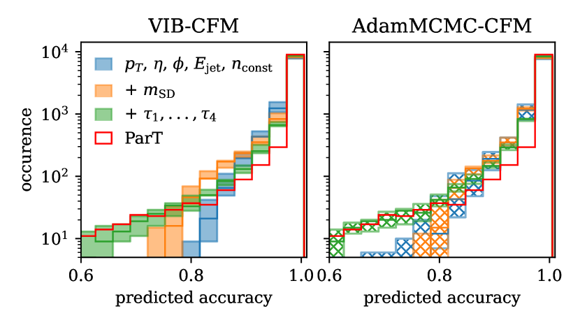
Figure 5: Accuracy of $1000$ ParT outputs predicted for each of $10000$ jet events. The different colors indicate the output of CNFs conditioned with increasing amount of features and thus provided with more information during inference. A histogram of the probabilistic ParT prediction itself is given in red.

JSD	VIB-CFM	AdamMCMC-CFM
$p_{T}$, $\eta$, $\phi$, $E_{\mathrm{jet}}$, $n_{\mathrm{const}}$	$0.174\pm 0.018$	$0.147\pm 0.036$
+ $m_{\mathrm{SD}}$	$0.134\pm 0.023$	$0.160\pm 0.013$
+ $\tau_{1},...,\tau_{4}$	$0.080\pm 0.009$	$0.097\pm 0.007$

Table 1: Jensen-Shannon-divergences between the histograms of predicted accuracies of Classifier Surrogates with different input features (Figure 5) and the actual accuracy distribution of the ParT.

5.2 Out-of-Distribution (OOD)

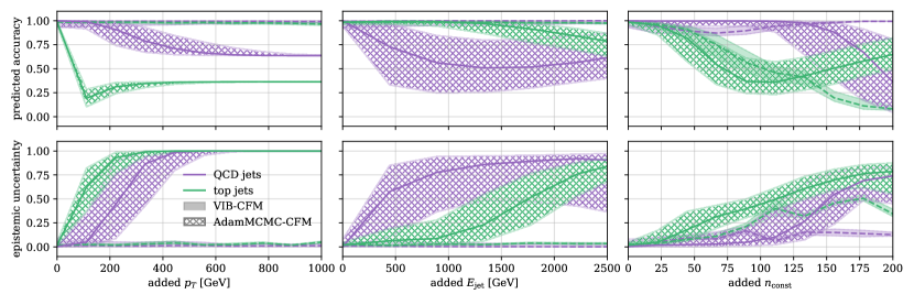
Figure 6: Behaviour of the Classifier Surrogate predictions for distorted input over the size of the distortion artificially added to the given jet-observable for $1000$ random events. The first row shows the accuracy predicted per event while the second row gives the mean epistemic uncertainty per event. Solid lines give the median of the set of events. The shaded and structured areas indicate the $10\%$-$90\%$-quantile envelope of the VIB and AdamMCMC ensemble respectively.

Although including an epistemic uncertainty into the evaluation this far is a nice feature to gauge uncertainties in the tail regions of the data, the true value of the Bayesian methods is indicating input that is outside the distribution of the training data through high uncertainties. We use the introduced measures (13) and (14) to show the behaviour of the Bayesian network for OOD data generated when artificially increasing the values for one jet-observable.

We produce OOD data by selecting $1000$ jet events from the test set at random and increasing the values of a single jet-feature by adding a constant value. We perform this distortion for $3$ dimensions, $p_{T}$, $E_{\mathrm{jet}}$ and $n_{\mathrm{const}}$, and $10$ values each. Again, we report the accuracy and error estimate calculated from $n_{\mathrm{stat}}=1000$ points of the learned Detector Smearing Distribution.

The first row of Figure 6 shows the mean accuracy predicted for the OOD data by the different drawings from the weight posterior. The envelope and solid line give the $10\%$- and $90\%$-quantile and the median over the set of events. When adding an unphysical offset to the features, we can see the mean predicted accuracy of the AdamMCMC ensemble rapidly drops. Optimally, the network predicts $0.5$ when all inputs are outside the training interval to indicate equal confidence of both classes. The ensemble seems to be able to detect most outliers, but only indicates large distortions of $E_{\mathrm{jet}}$ for top jets and of $n_{\mathrm{const}}$ for QCD jets.

The predicted accuracy of the VIB samples does not exhibit any dependence on the increasing offset in the OOD data. It is sensitive only to the number of jet constituents for top jets.

In the second row, we show the error estimate based on the difference between highest and lowest proposed output in the ensemble, see Equation 13. This measure captures the differences in the output and thus the encoded uncertainty directly. We expect increasing uncertainties for increasing offset. Only the AdamMCMC ensemble shows this behaviour, for all three disturbed input dimensions, while VIB once again is only sensitive to OOD inputs in the particle number. While the predicted accuracy did not capture the decreasing confidence for distorted $E_{\mathrm{jet}}$ of top jets well, the error estimate clearly indicates the unknown inputs. Similarly, distortions in $n_{\mathrm{const}}$ of QCD jets appear earlier in this measure.

6 Conclusion

In this paper, we proposed a first architecture for training Classifier Surrogates, Which are models describing the output of a deep neural network classification based on detector-level information from high-level jet observables and truth information. We show that the resulting Classifier Surrogates are well calibrated and scale with the amount of information provided. A novel combination with Monte Carlo generated samples from the networks Bayesian weight posterior allows for stable uncertainty quantification, that incorporates the density of the training data towards the edges. The predicted uncertainty reliable indicates unknown inputs.

This approach should next be implemented by the large experimental collaborations to allow the statistical re-interpretation of analysis results.

Acknowledgements

We thank the organisers and participants of the Les Houches – PhysTeV 2023 workshop for the stimulating environment which led to the idea for this work.

Furthermore, we thank Joschka Birk for helping with data preparation in the early stages of the work.

Declarations

Code

The training and evaluation code is available from https://github.com/sbieringer/ClassificationSurrogates and an example on handeling the JetClass dataset is given in https://github.com/joschkabirk/jetclass-top-qcd.

Funding

SB is supported by the Helmholtz Information and Data Science Schools via DASHH (Data Science in Hamburg - HELMHOLTZ Graduate School for the Structure of Matter) with the grant HIDSS-0002. SB and GK acknowledge support by the Deutsche Forschungsgemeinschaft (DFG) under Germany’s Excellence Strategy – EXC 2121 Quantum Universe – 390833306. JK is supported by the Alexander-von-Humboldt-Stiftung. This research was supported in part through the Maxwell computational resources operated at Deutsches Elektronen-Synchrotron DESY, Hamburg, Germany.

References

- \bibcommenthead
- Guest et al. [2018] Guest, D., Cranmer, K., Whiteson, D.: Deep Learning and its Application to LHC Physics. Ann. Rev. Nucl. Part. Sci. 68, 161–181 (2018) https://doi.org/10.1146/annurev-nucl-101917-021019 arXiv:1806.11484 [hep-ex]
- Albertsson et al. [2018] Albertsson, K., et al.: Machine Learning in High Energy Physics Community White Paper. J. Phys. Conf. Ser. 1085(2), 022008 (2018) https://doi.org/10.1088/1742-6596/1085/2/022008 arXiv:1807.02876 [physics.comp-ph]
- Radovic et al. [2018] Radovic, A., et al.: Machine learning at the energy and intensity frontiers of particle physics. Nature 560(7716), 41–48 (2018) https://doi.org/10.1038/s41586-018-0361-2
- Karagiorgi et al. [2021] Karagiorgi, G., Kasieczka, G., Kravitz, S., Nachman, B., Shih, D.: Machine Learning in the Search for New Fundamental Physics (2021) arXiv:2112.03769 [hep-ph]
- Kraml et al. [2012] Kraml, S., et al.: Searches for New Physics: Les Houches Recommendations for the Presentation of LHC Results. Eur. Phys. J. C 72, 1976 (2012) https://doi.org/10.1140/epjc/s10052-012-1976-3 arXiv:1203.2489 [hep-ph]
- Abdallah et al. [2020] Abdallah, W., et al.: Reinterpretation of LHC Results for New Physics: Status and Recommendations after Run 2. SciPost Phys. 9(2), 022 (2020) https://doi.org/10.21468/SciPostPhys.9.2.022 arXiv:2003.07868 [hep-ph]
- Araz et al. [2023] Araz, J.Y., et al.: Les Houches guide to reusable ML models in LHC analyses (2023) arXiv:2312.14575 [hep-ph]
- Guest et al. [2022] Guest, D.H., et al.: Lwtnn/lwtnn: Version 2.13. https://doi.org/10.5281/zenodo.6467676
- [9] Open Neural Network Exchange. https://onnx.ai
- ATLAS collaboration [2021] ATLAS collaboration: Search for R-parity-violating supersymmetry in a final state containing leptons and many jets with the ATLAS experiment using proton–proton collision data. Eur. Phys. J. C 81(11), 1023 (2021) https://doi.org/10.1140/epjc/s10052-021-09761-x arXiv:2106.09609 [hep-ex]
- ATLAS collaboration [2023] ATLAS collaboration: Search for supersymmetry in final states with missing transverse momentum and three or more b-jets in 139 fb-1 of proton–proton collisions at TeV with the ATLAS detector. Eur. Phys. J. C 83(7), 561 (2023) https://doi.org/10.1140/epjc/s10052-023-11543-6 arXiv:2211.08028 [hep-ex]
- ATLAS collaboration [2022] ATLAS collaboration: Search for neutral long-lived particles in collisions at = 13 TeV that decay into displaced hadronic jets in the ATLAS calorimeter. JHEP 06, 005 (2022) https://doi.org/10.1007/JHEP06(2022)005 arXiv:2203.01009 [hep-ex]
- ATLAS collaboration [2023] ATLAS collaboration: Anomaly detection search for new resonances decaying into a Higgs boson and a generic new particle in hadronic final states using TeV collisions with the ATLAS detector. Phys. Rev. D 108, 052009 (2023) https://doi.org/10.1103/PhysRevD.108.052009 arXiv:2306.03637 [hep-ex]
- ATLAS collaboration [2016] ATLAS collaboration: Performance of -Jet Identification in the ATLAS Experiment. JINST 11(04), 04008 (2016) https://doi.org/10.1088/1748-0221/11/04/P04008 arXiv:1512.01094 [hep-ex]
- CMS collaboration [2018] CMS collaboration: Identification of heavy-flavour jets with the CMS detector in pp collisions at 13 TeV. JINST 13(05), 05011 (2018) https://doi.org/10.1088/1748-0221/13/05/P05011 arXiv:1712.07158 [physics.ins-det]
- Qu et al. [2022a] Qu, H., Li, C., Qian, S.: Particle Transformer for Jet Tagging. In: Proceedings of the 39th International Conference on Machine Learning, pp. 18281–18292 (2022)
- Qu et al. [2022b] Qu, H., Li, C., Qian, S.: JetClass: A Large-Scale Dataset for Deep Learning in Jet Physics. https://doi.org/10.5281/zenodo.6619768
- Larkoski et al. [2014] Larkoski, A.J., Marzani, S., Soyez, G., Thaler, J.: Soft Drop. JHEP 05, 146 (2014) https://doi.org/10.1007/JHEP05(2014)146 arXiv:1402.2657 [hep-ph]
- Thaler and Van Tilburg [2011] Thaler, J., Van Tilburg, K.: Identifying Boosted Objects with N-subjettiness. JHEP 03, 015 (2011) https://doi.org/10.1007/JHEP03(2011)015 arXiv:1011.2268 [hep-ph]
- Badger et al. [2023] Badger, S., et al.: Machine learning and LHC event generation. SciPost Phys. 14(4), 079 (2023) https://doi.org/10.21468/SciPostPhys.14.4.079 arXiv:2203.07460 [hep-ph]
- Hashemi and Krause [2023] Hashemi, H., Krause, C.: Deep Generative Models for Detector Signature Simulation: An Analytical Taxonomy (2023) arXiv:2312.09597 [physics.ins-det]
- Winkler et al. [2019] Winkler, C., Worrall, D.E., Hoogeboom, E., Welling, M.: Learning likelihoods with conditional normalizing flows. CoRR (2019) arXiv:1912.00042 [cs.lg]
- Radev et al. [2020] Radev, S.T., Mertens, U.K., Voss, A., Ardizzone, L., Köthe, U.: Bayesflow: Learning complex stochastic models with invertible neural networks. IEEE transactions on neural networks and learning systems 33(4), 1452–1466 (2020) arXiv:2003.06281 [stat.ML]
- Chen et al. [2018] Chen, R.T., Rubanova, Y., Bettencourt, J., Duvenaud, D.K.: Neural ordinary differential equations. Advances in neural information processing systems 31 (2018) arXiv:1806.07366 [cs.LG]
- Rezende and Mohamed [2015] Rezende, D., Mohamed, S.: Variational inference with normalizing flows. In: International Conference on Machine Learning, pp. 1530–1538 (2015). PMLR
- Lipman et al. [2023] Lipman, Y., Chen, R.T.Q., Ben-Hamu, H., Nickel, M., Le, M.: Flow matching for generative modeling. In: The Eleventh International Conference on Learning Representations (2023)
- Blundell et al. [2015] Blundell, C., Cornebise, J., Kavukcuoglu, K., Wierstra, D.: Weight uncertainty in neural network. In: International Conference on Machine Learning, pp. 1613–1622 (2015). PMLR
- Butter et al. [2023] Butter, A., et al.: Jet Diffusion versus JetGPT – Modern Networks for the LHC (2023) arXiv:2305.10475 [hep-ph]
- Kingma and Ba [2014] Kingma, D.P., Ba, J.: Adam: A method for stochastic optimization. CoRR (2014) arXiv:1412.6980 [cs.LG]
- Bieringer et al. [2023] Bieringer, S., Kasieczka, G., Steffen, M.F., Trabs, M.: AdamMCMC: Combining Metropolis adjusted Langevin with momentum-based optimization (2023) arXiv:2312.14027 [stat.ML]