Controlling Markovianity with Chiral Giant Atoms

Abstract

A recent experimental work has demonstrated the chiral behavior of a giant artificial atom coupled to a microwave photonic waveguide. This is made possible through the engineering of complex phases in the two non-local couplings of the artificial atom to the waveguide. When the phase difference between the couplings and the accumulated optical phase between the coupling points are judiciously tuned, maximal chirality is achieved. In parell, giant atoms coupled to a waveguide are paradigmatic setups to observe non-Markovian dynamics due to self-interference effects. Here we report on a novel effect in giant atom physics that solely depends on the complex phases of the couplings. We show that, by adjusting the couplings’ phases, a giant atom can, counterintuitively, enter the Markovian regime irrespectively of any inherent time delay.

Introduction

The growing demand to process a significant amount of quantum information for computational purposes underscores the increasing importance of developing scalable quantum networks. These networks consist of spatially distributed nodes interconnected by communication lines. Consequently, investigating the realm where memory effects and quantum feedback are not negligible becomes increasingly crucial in addressing the challenge of quantum computation Lorenzo et al. (2013); Ramos et al. (2016); Haase et al. (2018); Fang et al. (2018); Milz et al. (2020); White et al. (2020); Tserkis et al. (2023).

The fine control of delayed quantum circuits and their theoretical description pose considerable challenges. Nevertheless, quantum feedback systems can showcase characteristics that are unattainable when interactions are strictly local. A notable instance includes multi-local or giant atoms Kannan et al. (2020); Frisk Kockum (2020); Cilluffo et al. (2020a); Leonforte et al. (2024), which are two-level emitters coupled to an environment (such as a field flowing through a waveguide) at multiple spatially separated points. As the light travels among these distinct coupling points, it accumulates a phase (optical length) $\varphi_{\text{WG}}$ proportional to the distance between them. When the coupling points are spaced at distances comparable to the wavelength of the light they interact with, a direct consequence of the phase accumulation is that self-interference effects, absent in quantum optics with ordinary atoms, arise.

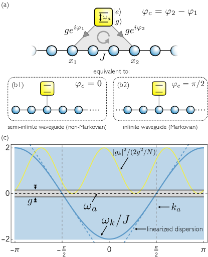
Figure 1: Setup. (a) Chiral giant atom coupled at the points $x_{1,2}$ to a 1D bidirectional waveguide. The couplings are generally complex with phases $\varphi_{1,2}$, cf. Eq. (2). When $\varphi_{c}=\pi/2$ [$\varphi_{c}=0$], as in (b2) [(b1)], the system is equivalent to a small atom (local coupling) in a [semi-]infinite waveguide and the dynamics is [non-]Markovian. (c) Dispersion law of the waveguide (solid blue), which in weak coupling (gray stripe) can be linearized (dashed blue). The atomic frequency $\omega_{a}=0$ is resonant with the middle of the band, corresponding to the momentum $k_{a}=\pi/2$. In yellow we show an instance of the atom-waveguide coupling as in Eq. (3) with $L=2$, $x_{2}-x_{1}=3$ and $\varphi_{c}=\pi/6$, showing the chirality ($|g_{k_{a}}|>|g_{-k_{a}}|$).

A remarkable feature of giant atoms is their non-Markovian character. Indeed, a giant atom can reabsorb its own emitted excitation after a time delay proportional to the distance between the coupling points. This phenomenon has been experimentally demonstrated, first with superconducting qubits coupled to surface acoustic waves Andersson et al. (2019), and was one of the main motivation that spurred the interest in giant atoms physics. Interestingly, as we detail below, a giant atom coupled to a waveguide at two different coupling points can be described in terms of a small atom (one coupling point) in front of a mirror, that is a semi-infinite waveguide, Fig. 1(a-b1), the latter being a typical setup to observe a non-Markovian behavior of the atomic emission Tufarelli et al. (2013, 2014); González-Tudela and Cirac (2017).

Another striking feature of giant atoms is the possibility of engineering decoherence-free interactions between them upon the specific pattern of the coupling points to a waveguide Kockum et al. (2018). Remarkably, even if the latter effect is inherently related to the phase differences associated to the displacements of the coupling points, it becomes prominent when the travel time of light between coupling points is small compared to the characteristic time scales of the emitters, i.e., in the Markovian limit Kockum et al. (2018); Carollo et al. (2020a).

In parallel to the relevance of memory effects, another important aspect concerns the potential to adjust the propagation direction of light between the nodes. When scattered radiation displays a preferred direction, the interaction between emitters and light is defined as chiral Lodahl et al. (2017). Both theoretically Ramos et al. (2016) and very recently experimentally Joshi et al. (2023) it has been shown that introducing light-matter couplings with an additional complex phase can induce a chiral behaviour in the radiation emitted by giant atoms. For a giant atom with two coupling points, cf. Fig. 1(a), the atomic emission is chiral whenever the phase difference between the couplings $\varphi_{c}$ does not vanish. In particular, when such a phase matches the optical length $\varphi_{\rm WG}$, the emission can become maximally chiral (that is, inhibited in either the forward or backward direction). Importantly, maximal chirality results from the right matching of the optical length and the phase difference of the giant atom’s couplings Ramos et al. (2016).

In this work, we bridge these two seemingly unrelated features of giant atoms, namely their chirality and their (non-)Markovianity. We find a simple recipe to make a giant atom enter the Markovian regime, even for non-negligible time delays, by tuning its chirality. Importantly, our result depends solely on the complex nature of the atom-light couplings. Our result contributes to the ongoing debate on whether an atom is deemed “giant” due to non-Markovianity or the non-local nature of the couplings. Our analysis emphasizes that the crucial factor lies in the non-locality of the couplings.

Setup and Hamiltonian

We consider a single giant atom weakly coupled to a one-dimensional (1D) bidirectional waveguide. The full light-matter Hamiltonian is $\hat{H}=\hat{H}_{w}+\hat{H}_{a}+\hat{H}_{\text{int}}$. The free atomic Hamiltonian is $\hat{H}_{a}=\omega_{a}\hat{\sigma}^{\dagger}\hat{\sigma}$, with $\hat{\sigma}=\outerproduct{g}{e}$, $\ket{g}$ and $\ket{e}$ being the ground and excited atomic states, respectively. We model the waveguide with a uniform tight-binding array of coupled resonators with Hamiltonian

$$\hat{H}_{w}=-J\sum_{x}\hat{a}_{x+1}^{\dagger}\hat{a}_{x}+\text{ H.c.}\,$$ (1)

where $\hat{a}_{x}$ are real space bosonic annihilation operators and $J>0$. Assuming translational invariance, we can Fourier transform $\hat{a}_{x}=\sum_{k}e^{-ikx}\hat{a}_{k}/\sqrt{N}$, where $N$ is the number of resonators, so that the Eq. (1) reads $\hat{H}_{w}=\sum_{k}\omega_{k}\hat{a}_{k}^{\dagger}\hat{a}_{k}$, with $\omega_{k}=-2J\cos k$ (the lattice constant is set to 1). The atom-waveguide interaction Hamiltonian reads

$$\hat{H}_{\text{int}}=g\hat{\sigma}\left(\sum_{j=1}^{L}e^{i\varphi_{j}}\hat{a}_{x_{j}}^{\dagger}\right)+\text{ H.c.}\,,$$ (2)

where we assume $g$ to be real, $\varphi_{1}$ to vanish (as it can be gauged away), and $x_{j}=x_{1}+(j-1)d$ for $j=1,\dots,L$, so that the coupling points are equally spaced. The assumption of weak coupling makes this system equivalent to a continuous waveguide with linear dispersion Shen and Fan (2009), see Fig. 1(c). From an experimental point of view, our waveguide Hamiltonian can be implemented with a continuous transmission line Joshi et al. (2023), as well as with an array of coupled superconducting circuits Kim et al. (2021); Scigliuzzo et al. (2022); Zhang et al. (2023). In Fourier space the interaction Hamiltonian (2) reads $\hat{H}_{\text{int}}=\sum_{k}g_{k}\,\hat{\sigma}\hat{a}_{k}^{\dagger}+\text{H.c.}$, where

$$g_{k}=\frac{g}{\sqrt{N}}\sum_{j=1}^{L}e^{i(\varphi_{j}+kx_{j})}\,.$$ (3)

When all these phases are zero, we refer to the giant atom as non-chiral. By contrast, we will call the giant atom chiral whenever we take into account non-zero phases. This is because, in the latter case, time reversal symmetry is broken ($g_{k}\neq g_{-k}$ in general). In the following we focus on two-legged giant atoms, leaving the general case to the end of the paper.

Result

Our result can be condensed in the following sentence: the chirality of a giant atom controls its Markovianity. Remarkably, when the phase difference between the couplings is exactly $\pi/2$, Markovianity is achieved irrespectively of any time delay. This implies that such a chiral giant atom undergoes spontaneous emission even when the coupling points are significantly far apart, and therefore when reabsorption would occur in the non-chiral case. Despite the atom being giant, in the sense that a non-Markovian behavior is expected, it behaves as if it were small. Thus, we argue in favor of the non-locality of the couplings as a defining feature of giant atoms.

We derive this result through the analytic calculation of the exact atomic dynamics and further check it through the Lindblad master equation. We then provide two mechanisms for this phenomenon, based on an interference argument and on a collision model picture Ciccarello et al. (2022); Ciccarello (2018); Cilluffo et al. (2020b).

Assume the initial state is $\ket{\Psi(0)}=\ket{e}\!\ket{0}$, $\ket{0}$ being the vacuum state of the field. Then at time $t$ the full atom-waveguide state is $\ket{\Psi(t)}=\varepsilon(t)\ket{e}\!\ket{0}+\sum_{k}\,c_{k}(t)\,\hat{a}_{k}^{\dagger}\ket{g}\!\ket{0}\,.$ Imposing the Schrödinger equation, the dynamics of an initially excited chiral giant atom follows the delay differential equation (see Appendix A)

$$\dot{\varepsilon}(t)=-\frac{\Gamma}{2}\varepsilon(t)-\frac{\Gamma}{2}\cos(\varphi_{c})e^{i\varphi_{\text{WG}}}\Theta(t-t_{d})\varepsilon(t-t_{d})\,.$$ (4)

Here, $\Theta(t)$ is the Heaviside step function, $\varphi_{\text{WG}}$ is the optical length between the coupling points, $t_{d}$ is the corresponding time delay, and $\Gamma$ is the decay rate. More specifically, the optical length is given by $\varphi_{\text{WG}}=k_{a}d$ where $d$ is the distance between the coupling points, $k_{a}$ is the momentum corresponding to the atomic transition frequency $\omega_{a}$ ($k_{a}=\pi/2$ in our case), $v=2J\sin(k_{a})$ is the speed of light in the waveguide, and $\Gamma=4g^{2}/v$.

For $\varphi_{c}=0$, Eq. (4) is well known Tufarelli et al. (2013), and indeed shows the analogy between a non-chiral giant atom and a small atom in front of a mirror, cf. Fig. 1(a-b1). The only difference with Ref. Tufarelli et al. (2013) is the minus sign in front of the second term in the right hand side of Eq. (4). Such $\pi$ phase difference is due to the fact that in Ref. Tufarelli et al. (2013) the optical length is proportional to twice the distance between the atom and the mirror, as light has to hit the mirror and come back.

Interestingly, we observe that the atomic decay is exactly exponential at $\varphi_{c}=\pi/2$, regardless of the time delay $t_{d}$, matching the behavior of a small atom coupled (with scaled coupling strength) to a waveguide. By contrast, the non-Markovianity of a chiral giant atom is prominent when $\varphi_{\text{WG}}=m\pi$ and $\varphi_{c}=(m+1)\pi$ with integer $m\geq 0$ (matching, for odd $m$, the result in Ref. Tufarelli et al. (2013)). At these values, part of the emitted light is trapped between the coupling points forming a bound state in the continuum (BIC) Hsu et al. (2016); Calajó et al. (2019). In Fig. 2, we show the dynamics of an initially excited chiral giant atom, which indeed decays exponentially, regardless of the time delay, for $\varphi_{c}=\pi/2$.

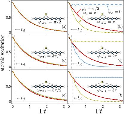
Figure 2: Markovianity for any time delay. Dynamics of the atomic excitation, $|\varepsilon(t)|^{2}$, of an initially excited chiral giant atom for various distances $d$ between the coupling points, corresponding to various optical lengths $\varphi_{\text{WG}}=k_{a}d$ and phase differences $\varphi_{c}$ between the couplings to the waveguide. Specifically, $d=1,2,3,4,5,6$ in (a-f), respectively. In all panels (a-f) $\varphi_{c}=0,\pi/2,\pi$ correspond to blue, red and dashed yellow, respectively. The black dotted lines represent the exact exponential decay $e^{-\Gamma t}$, while the other curves are obtained numerically. Regardless of the time delay $t_{d}=d/v$, dashed grey, increasing from (a) to (f), at $\varphi_{c}=\pi/2$ the decay is exactly exponential. When the optical length is an integer multiple of $\pi$, the atom never fully decays and correspondingly a BIC occur. On top of the BICs occurring at odd multiples of $\pi$ for a non-chiral giant atom, (b) and (f), as in Ref. Tufarelli et al. (2013), complex couplings allow the appearance of BICs at even multiples of $\pi$ as well (see Appendix D). Other parameter values: $k_{a}=\pi/2$, $g=0.2J$, $v=2J$, $N=90$ (number of resonators), the first (second) coupling point is at $N/2$ ($N/2+d$).

Beyond the exact treatment, this behavior can be captured as well through the atomic master equation for small distances between the coupling points, when the Markov approximation is still valid. In the derivation of the master equation, this approximation makes the evolution of the density matrix time-local. Notwithstanding, the interaction Hamiltonian still keeps track of the non-locality of the atom-light interaction. The atomic master equation reads $\dot{\rho}=-i[\hat{H}_{a},\rho]+\gamma\left(\hat{\sigma}\rho\hat{\sigma}^{\dagger}-\{\hat{\sigma}^{\dagger}\hat{\sigma},\rho\}/2\right)$ where (see Appendix B)

$$\gamma=\Gamma\left[1+\cos(\varphi_{c})\cos(k_{a}d)\right]\,.$$ (5)

This matches the exact result, predicting an exponential decay with rate $\Gamma$ for $\varphi_{c}=\pi/2$ . The same rate is obtained for $k_{a}d=\pi/2$ (and odd multiples), which, for our discretized waveguide, corresponds to odd distances $d$. Indeed, in Fig. 2 we see that for odd $d$’s the decay is almost exponential for any complex phase $\varphi_{c}$ (the discrepancy increases with $d$ as the Markov approximation gets worse).

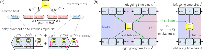
Figure 3: Mechanism of Markovianity for any time delay. (a) Interference picture. At each coupling point ($x_{1}$, $x_{2}$) the emitted field can be divided into forward and backward components (right- and left-pointing blue and red arrows, respectively) $c_{1,\text{f}}(t)$ and $c_{1,\text{b}}(t)$ (same for $x_{2}$). For $t\geq t_{d}=d/v$, $d=x_{2}-x_{1}$, the forward [backward] component at the coupling point $x_{2}$ [$x_{1}$] acquires a delay contribution $c_{2,\text{f}}^{\text{del}}(t)$ [$c_{1,\text{b}}^{\text{del}}(t)$] (light blue arrows), as the atomic excitation (small fuchsia circle) is transferred by hopping via the $x_{1}$ [$x_{2}$] coupling point and travelling along the waveguide for a distance $d$. A non-Markovian behavior takes place only if the atom gets re-excited. The amplitude for this process to occur is the sum of the two possible ways for the re-excitation to happen, as illustrated at the bottom part. Considering the phases aquired along these two paths, the final amplitude is proportional to $\cos(\varphi_{c})$. (b) Collision model picture. Left- and right-going field modes (top and bottom, respectively) are mapped into trains of time-bin ancillae moving in opposite directions. At each time step the system interacts with two separated ancillae from each bath and the chains are shift by one position. After the first collision, each ancilla will interact again with the system in $\ell$ steps. When the complex phase $\varphi_{c}=\pi/2$ (and odd multiples) this picture is unitarily equivalent to a Markovian collision model where the system interacts locally with the two left- and right- going time bins of a bidirectional waveguide.

Mechanism

First, the exponential atomic decay at $\varphi_{c}=\pi/2$ can be explained as an interference effect. The key observation is that the phases $\varphi_{1,2}$ and $\varphi_{\text{WG}}$ have to be considered with and without their signs, respectively. Indeed, $\varphi_{\text{WG}}$ is always positive regardless of the interference path, while $\varphi_{c}$ is positive (negative) sign when going from the atom (field) to the field (atom).

At the left and right coupling points, $(x_{1},x_{2})$, we can write the emitted field amplitude at time $t$ as $c_{1,2}(t)$ (see Appendix C). We can further divide these terms into backward (to the left) and forward (right) emitted field amplitude $c_{1}(t)=c_{1,\text{b}}(t)+c_{1,\text{f}}(t)$, analogously for $c_{2}(t)$. As the atom is coupled at the two points $x_{1}$ and $x_{2}$ to the waveguide, the backward emitted field at coupling point $x_{1}$ has (i) a contribution coming directly from the atomic exponential decay, and (ii) a contribution coming from the backward emitted field at coupling point $x_{2}$. Thus, we can further divide $c_{1,\text{b}}(t)$ into its exponential (exp) and delay (del) contributions as $c_{1,\text{b}}(t)=c_{1,\text{b}}^{\text{del}}(t)+c_{1,\text{b}}^{\text{exp}}(t)$ and $c_{2,\text{f}}(t)=c_{2,\text{f}}^{\text{exp}}(t)+c_{2,\text{f}}^{\text{del}}(t)$ (the same goes for the forward emitted field at coupling point $x_{2}$). Note that $c_{1,\text{b}}^{\text{del}}(t)=c_{2,\text{f}}^{\text{del}}(t)=0$ for $t<t_{d}$.

On the one hand, the only way to increase the atomic amplitude $\varepsilon$ is via the field contribution coming from the delay, which is (we drop the time dependence to lighten notation)

$$c_{1,\text{b}}^{\text{del}}\,e^{-i\varphi_{1}}+c_{2,\text{f}}^{\text{del}}\,e^{-i\varphi_{2}}\,.$$ (6)

On the other hand, the atomic population contribution to these field components is

$$c_{1,\text{b}}^{\text{del}}=e^{i\varphi_{2}}\,e^{i\varphi_{\text{WG}}}\,\varepsilon,\quad c_{2,\text{f}}^{\text{del}}=e^{i\varphi_{1}}\,e^{i\varphi_{\text{WG}}}\,\varepsilon\,.$$ (7)

By plugging Eqs. (7) into Eq. (6), the delay contribution to the atomic amplitude turns out to be proportional to $\cos(\varphi_{c})$. Therefore, for $\varphi_{c}=\pi/2$ there is no delay contribution, and the atomic excitation decays exactly exponentially irrespectively of any distance between coupling points. This interference effect is illustrated in Fig. 3(a).

Second, in the framework of collision models Ciccarello et al. (2022), the time-evolution of the atom and the waveguide is described as a sequence of discrete interactions (collisions) involving the system (the atom) and discretized field modes (referred to as ancillae or time bin modes). In the case of a giant atom, the interaction involves two separated ancillae, see Fig. 3(b). A non-Markovian behaviour typically arises due to the double interaction between the system and the same ancilla after a finite time. For a single giant atom with two legs ($L=2$), the coupling Hamiltonian (2) in interaction picture with respect to the waveguide and the atom reads

$$\hat{H}_{\rm int}(t) = g\,\,\hat{\sigma}^{\dagger}[e^{-ik_{a}x_{1}}\,{\hat{a}}_{t-\tau_{1}}+e^{ik_{a}x_{1}}\,\hat{a}^{\prime}_{t+\tau_{1}}$$ (8)

$$+e^{i\varphi_{c}}(e^{-ik_{a}x_{2}}\,{\hat{a}}_{t-\tau_{2}}+e^{ik_{a}x_{2}}\,{\hat{a}}^{\prime}_{t+\tau_{2}})]$$

$$+{\rm H.c.}$$

Without loss of generality we have set $\varphi_{1}=0$ and thus $\varphi_{2}=\varphi_{c}$. In Eq. (8), ${\hat{a}}_{t-\tau_{1,2}}({\hat{a}}^{\prime}_{t+\tau_{1,2}})$ are the right- (left-) going time bin operators corresponding to coupling points $x_{1,2}$ Carollo et al. (2020b), and $\tau_{1,2}=x_{1,2}/v$ are the time-domain coordinates corresponding to the coupling points’ positions. The left-going operators have a prime to stress the distinction with the right-going ones (below it will be clear why such an additional distinction is needed). For an infinitesimal evolution time $\Delta t$, the related propagator is approximated as $\mathcal{\hat{U}}_{n}\simeq\mathbb{1}-i(\hat{\mathcal{H}}_{n}^{(0)}+\hat{\mathcal{H}}_{n}^{(1)})\Delta t-(\hat{\mathcal{H}}_{n}^{(0)})^{2}\Delta t^{2}/2$, where $\hat{\mathcal{H}}_{n}^{(0)}=\tfrac{1}{\Delta t}\!\int_{t_{n-1}}^{t_{n}}\text{d}s\,\hat{H}_{\rm int}(s)$ and $\hat{\mathcal{H}}_{n}^{(1)}=\tfrac{i}{2\Delta t}\!\int_{t_{n-1}}^{t_{n}}\!\text{d}s\int_{t_{n-1}}^{s}\!\text{d}s^{\prime}\,[\hat{H}_{\rm int}(s^{\prime}),\hat{H}_{\rm int}(s)]$ are the $0$th and the $1$st order terms of the Magnus expansion of the generator Magnus (1954). The operators of both the emitter and the waveguide modes are present only in the $0$th-order term, i.e., only $\hat{\mathcal{H}}_{n}^{(0)}$ describes the interaction while $\hat{\mathcal{H}}_{n}^{(1)}$ is a Lamb-shift term. We thus write the former as

$$\hat{\mathcal{H}}_{n}^{(0)}= \,\,g\,\hat{\sigma}^{\dagger}[{\hat{a}}_{n}+e^{i\varphi_{c}}e^{-i\varphi_{\text{WG}}}\,{\hat{a}}_{n-\ell}\,+$$

$$\,\,{\hat{a}}_{n}^{\prime}+e^{i\varphi_{c}}e^{i\varphi_{\text{WG}}}\,{\hat{a}}_{n+\ell}^{\prime}]+{\rm H.c.}$$ (9)

where we introduced the right-going time-bin operators $\hat{a}_{n}=\tfrac{1}{\sqrt{\Delta t}}\int_{t_{n-1}}^{t_{n}}\!\text{d}t\,\hat{a}_{t}$ (the same holding for the left-going ones $\hat{a}_{n}^{\prime}$). Without loss of generality, we set $x_{1}=0$, $x_{2}=d$ and $\ell\Delta t=\tau_{2}$ (which is nothing but the time delay $t_{d}$). The relation (Mechanism) captures all the relevant physics of the atom-waveguide crosstalk in all regimes and makes clear the (general) non-Markovian nature of the dynamics.

Consider now a separate (Markovian) collision model of an emitter coupled to a bidirectional waveguide, whose $n$th collision is described by the Hamiltonian

$$\hat{h}_{n}^{(0)} =\sqrt{2}g\,\,\hat{\sigma}^{\dagger}(\hat{A}_{n}+\hat{A}_{n}^{\prime})+{\rm H.c.}\,,$$ (10)

where $\hat{A}_{n}$ and $\hat{A}_{n}^{\prime}$ are the right- and left- going time-bin operators, respectively. Setting $\hat{A}_{n}=(\hat{a}_{n}+e^{i(\varphi_{c}-\varphi_{\text{WG}})}\hat{a}_{n-\ell})/\sqrt{2}$ and $\hat{A}_{n}^{\prime}=(\hat{a}_{n}^{\prime}+e^{i(\varphi_{c}+\varphi_{\text{WG}})}\hat{a}_{n+\ell}^{\prime})/\sqrt{2}$, these transformations define the unitary input-output relations for a beam splitter Loudon (2000), if and only if $\varphi_{c}=\pi/2$ (see Appendix E).

Therefore, for $\varphi_{c}=\pi/2$, there exists an exact mapping between Eq. (Mechanism) (generally non-Markovian) and Eq. (10) (Markovian). Under this condition, the transformation does not alter the reduced dynamics of the system. This leads to the conclusion that the collision model describing a chiral giant atom with an arbitrary delay line between its legs becomes equivalent to a collision model where the atom interacts with the field at a single point with a rescaled coupling strength. Significantly, this implies that the reduced dynamics of the system is exactly Markovian, even in the presence of any time delay.

Finally, we note how the collision model picture provides a simple explanation of the chirality of the emission given by a complex coupling Ramos et al. (2016). In the case $\varphi_{\text{WG}}=\pi/2$ (necessary for maximal chiral emission) and in the negligible-time-delay limit $(\ell\sim 0)$, Eq. (Mechanism) reduces to

$$\hat{\mathcal{H}}_{n}^{(0)}=g\,\hat{\sigma}^{\dagger}[(1-ie^{i\varphi_{c}}){\hat{a}}_{n}+(1+ie^{i\varphi_{c}})\,{\hat{a}}_{n}^{\prime}]+{\rm H.c.}$$

Hence, adjusting the complex phase $\varphi_{c}$ enables control over the chirality of the emission. Specifically, when $\varphi_{c}=\pi/2$, emission to the left-going modes is inhibited, in agreement with the results in Refs. Ramos et al. (2016); Joshi et al. (2023).

Generalization to multiple coupling points

A Markovian behavior can be achieved as well with $L>2$ coupling points by properly tuning the $L-1$ complex phases $\varphi_{2},\ldots,\varphi_{L}$. It turns out (see Appendix F) that the conditions they have to satisfy are

$$\sum_{j=1}^{L-n}\cos(\varphi_{n+j}-\varphi_{j})=0,\qquad\,n=1,\ldots,L-1,$$ (11)

where for convenience we restored $\varphi_{1}$. When Eqs. (11) are satisfied, the decay rate of the giant atom is $Lg^{2}/v$, namely $L$ times the rate of a small atom in a waveguide.

A general solution to these coupled equations is not informative on its own, rather we notice that one can always solve the last one ($n=L-1$), finding $\varphi_{L}=\pi/2$, plugging it back in the second to last one ($n=L-2$), and recursively find a solution to all of them. For instance, with three coupling points ($L=3$), we find a Markovian bahavior by setting $\varphi_{3}=\pi/2$ and $\varphi_{2}=-\pi/4$, while with four coupling points ($L=4$) one can set $\varphi_{4}=\varphi_{2}=\pi/2$ and $\varphi_{3}=\pi$.

Conclusion

An artificial atom coupled at multiple points to a waveguide is a paradigmatic setup to observe memory effects due to self-intereference. We have found that this paradigm can break down when the atom-light couplings are allowed to be complex. By properly adjusting the coupling phases, the artificial atom has an exact Markovian behavior, regardless of any inherent time delay involved in the dynamics. This unexpected effect enriches the already exotic physics of giant atoms, opening new theoretical and experimental avenues.

For instance, an important result in giant atoms physics is the occurrence of dispersive decoherence free interactions. However, we unveil here a novel effect, crucially dependent on complex atom-light couplings, that occurs in the opposite regime, i.e., far from protecting the atom from decoherence. The effect we find is relevant from the theoretical standpoint on its own. Indeed, many works righteously point out that time delays need to be neglected to derive a master equation for giant atoms in a waveguide Kockum et al. (2018); Kannan et al. (2020); Cilluffo et al. (2020b); Carollo et al. (2020b). Our result shows that, at least for a single giant atom, there is no need to make such approximation. Finally, we note that the effect we described could be tested in principle by coupling a transmon qubit either to a microwave photonic waveguide Kannan et al. (2020); Joshi et al. (2023), or to an array of superconducting LC circuits Scigliuzzo et al. (2022); Zhang et al. (2023).

Appendix A Derivation of the delay differential equation (4)

Here we derive the exact delay differential equation governing the time evolution of the amplitude of a two-legged chiral giant atom. We consider the case of multiple legs in Appendix F. The non-chiral case is recovered for $\varphi_{c}=0$. Assuming the initial state is $\ket{\Psi(0)}=\ket{e}\!\ket{0}$, the state at time $t$ will be

$$\ket{\Psi(t)}=\varepsilon(t)\ket{e}\!\ket{0}+\sum_{k}\,c_{k}(t)\,\hat{a}_{k}^{\dagger}\ket{g}\!\ket{0}.$$ (12)

Observe that the photonic amplitudes in real space are obtained as $c_{x}(t)=\sum_{k}e^{-ikx}c_{k}(t)/\sqrt{N}$. Imposing the Schrödinger equation, and making the replacements $\varepsilon(t)\rightarrow\varepsilon(t)e^{-i\omega_{a}t}$ and $c_{k}(t)\rightarrow c_{k}(t)e^{-i\omega_{a}t}$, we get the following equations for the atomic and photonic amplitudes

$$\dot{\varepsilon}(t) = -i\sum_{k}\,g_{k}^{*}c_{k}(t)\,,$$ (13)

$$\dot{c}_{k}(t) = -i(\omega_{k}-\omega_{a})c_{k}(t)-ig_{k}\varepsilon(t)\,,$$ (14)

with initial conditions $\varepsilon(0)=1$ and $c_{k}(0)=0$ for all $k$. Integrating Eq. (14) and plugging the result back in Eq. (13) we get

$$\dot{\varepsilon}(t)=-\int_{0}^{t}\text{d}s\varepsilon(s)e^{-i\omega_{a}(s-t)}\sum_{k}|g_{k}|^{2}e^{i\omega_{k}(s-t)}\,.$$ (15)

Now we compute explicitly the last term in previous equation (we set $\varphi_{1}=0$ so that $\varphi_{2}=\varphi_{c}$)

$$\sum_{k}|g_{k}|^{2}e^{i\omega_{k}(s-t)} = \frac{g^{2}}{N}\sum_{k}\left(2+e^{i(\varphi_{c}+kd)}+e^{-i(\varphi_{c}+kd)}\right)e^{i\omega_{k}(s-t)}$$

linearizing the waveguide dispersion because of weak coupling $$\omega_{k}\approx v|k|$$

$$= \frac{g^{2}}{N}\sum_{k}\left(2+e^{i(\varphi_{c}+kd)}+e^{-i(\varphi_{c}+kd)}\right)e^{iv|k|(s-t)}$$

separating positive and negative $$k d=vt_{d}$$’s and setting

$$= \frac{g^{2}}{N}\sum_{k>0}\left(2+e^{i(\varphi_{c}+kvt_{d})}+e^{-i(\varphi_{c}+kvt_{d})}\right)e^{ivk(s-t)}$$

$$+\frac{g^{2}}{N}\sum_{k<0}\left(2+e^{i(\varphi_{c}+kvt_{d})}+e^{-i(\varphi_{c}+kvt_{d})}\right)e^{-ivk(s-t)}$$

$$= \frac{g^{2}}{N}\sum_{k>0}\left(2e^{ivk(s-t)}+e^{i\varphi_{c}}e^{ivk(t_{d}+s-t)}+e^{-i\varphi_{c}}e^{-ivk(t_{d}-s+t)}\right)$$

$$+\frac{g^{2}}{N}\sum_{k<0}\left(2e^{-ivk(s-t)}+e^{i\varphi_{c}}e^{ivk(t_{d}-s+t)}+e^{-i\varphi_{c}}e^{-ivk(t_{d}+s-t)}\right)$$

extending the first (second) sum, which is taken around $$k_{a} -k_{a} k$$ (), to all ’s

$$= \frac{g^{2}}{N}\sum_{k}\left(2e^{ivk(s-t)}+e^{i\varphi_{c}}e^{ivk(t_{d}+s-t)}+e^{-i\varphi_{c}}e^{-ivk(t_{d}-s+t)}\right)$$

$$+\frac{g^{2}}{N}\sum_{k}\left(2e^{-ivk(s-t)}+e^{i\varphi_{c}}e^{ivk(t_{d}-s+t)}+e^{-i\varphi_{c}}e^{-ivk(t_{d}+s-t)}\right)$$

replacing $$k\rightarrow-k$$ in the second sum

$$= \frac{g^{2}}{N}\sum_{k}\left(2e^{ivk(s-t)}+e^{i\varphi_{c}}e^{ivk(t_{d}+s-t)}+e^{-i\varphi_{c}}e^{-ivk(t_{d}-s+t)}\right)$$

$$+\frac{g^{2}}{N}\sum_{k}\left(2e^{ivk(s-t)}+e^{i\varphi_{c}}e^{-ivk(t_{d}-s+t)}+e^{-i\varphi_{c}}e^{ivk(t_{d}+s-t)}\right)$$

$$= \frac{g^{2}}{N}\sum_{k}\left(4e^{ivk(s-t)}+2\cos(\varphi_{c})e^{ivk(t_{d}+s-t)}+2\cos(\varphi_{c})e^{-ivk(t_{d}-s+t)}\right)$$

$$\text{ setting $\Delta k=\frac{2\pi}{N}$, we get }\frac{1}{N}\sum_{k}e^{ivk(s-t)}=\frac{1}{2\pi}\sum_{k}e^{ivk(s-t)}\Delta k\rightarrow\int\frac{\text{d}k}{2\pi}\,e^{ivk(s-t)}=\frac{1}{v}\delta(s-t)$$

$$= \frac{g^{2}}{v}\left[4\delta(s-t)+2\cos(\varphi_{c})\delta(t_{d}+s-t)+2\cos(\varphi_{c})\delta(t_{d}-s+t)\right]\,,$$

where the limit is taken as $N\rightarrow\infty$. Finally, plugging the result back into Eq. (15) and performing the integration (recall that $\Theta(0)=1/2$) we get Eq. (4).

Appendix B Master equation of a two-legged chiral giant atom

Here we derive the chiral giant atom decay rate (5) through the GKSL master equation. The interaction Hamiltonian in interaction picture with respect to $\hat{H}_{a}+\hat{H}_{w}$ reads $\hat{H}_{I}(t)=e^{i\omega_{a}t}\hat{\sigma}^{+}\hat{B}(t)+\text{ H.c.}$, with $\hat{B}(t)=\sum_{k}g_{k}^{*}\hat{a}_{k}e^{-i\omega_{k}t}$. Notice that the information on the non-locality of the interaction is within $g_{k}$. Following the standard recipe Breuer and Petruccione (2007), the giant atom master equation reads as $\dot{\rho}=-i[\hat{H}_{a},\rho]+\gamma\left(\hat{\sigma}\rho\hat{\sigma}^{\dagger}-\{\hat{\sigma}^{\dagger}\hat{\sigma},\rho\}/2\right)$, where $\gamma=2\real[I(\omega_{a})]$ and

$$I(\omega_{a})=\int_{0}^{\infty}\text{d}\tau\langle\hat{B}(\tau)\hat{B}^{\dagger}(0)\rangle e^{i\omega_{a}\tau} \rightarrow 2g^{2}\int_{0}^{\infty}\text{d}\tau\int\frac{\text{d}k}{2\pi}[1+\cos(\varphi_{c}+kd)]e^{i(\omega_{a}-\omega_{k})\tau}$$ (17)

$$= 2g^{2}\int\frac{\text{d}k}{2\pi}[1+\cos(\varphi_{c}+kd)]\left[\pi\delta(\omega_{a}-\omega_{k})+i\mathcal{P}\frac{1}{\omega_{a}-\omega_{k}}\right]\,,$$

where the waveguide state is assumed to be the vacuum, the limit is takes as $N\rightarrow\infty$, and $\mathcal{P}$ denotes the principal value. Therefore, analogously to the steps taken to get Eq. (A), we get

$$\gamma = \frac{2g^{2}}{v}\int\text{d}k[1+\cos(\varphi_{c}+kd)]\delta(k_{a}-|k|)$$

$$= \frac{2g^{2}}{v}\int_{\{-k_{a}\}}\text{d}k[1+\cos(\varphi_{c}+kd)]\delta(k_{a}+k)+\frac{2g^{2}}{v}\int_{\{k_{a}\}}\text{d}k[1+\cos(\varphi_{c}+kd)]\delta(k_{a}-k)$$

$$= \frac{2g^{2}}{v}\int\text{d}k[1+\cos(\varphi_{c}+kd)]\delta(k_{a}+k)+\frac{2g^{2}}{v}\int\text{d}k[1+\cos(\varphi_{c}+kd)]\delta(k_{a}-k)$$

$$= \frac{2g^{2}}{v}[1+\cos(\varphi_{c}-k_{a}d)]+\frac{2g^{2}}{v}[1+\cos(\varphi_{c}+k_{a}d)]$$

$$= \frac{4g^{2}}{v}[1+\cos(\varphi_{c})\cos(k_{a}d)]\,.$$

On the one hand this shows that for $\varphi_{c}=\pi/2$ we get the exponential decay with the correct rate, independently on the distance between the coupling points. On the other hand, we get the same rate when $k_{a}d$ is an odd multiple of $\pi/2$. For small $d$ (i.e., when the Markovian approximation is more accurate), this matches the almost exponential decay we see in Fig. 2 for odd $d$’s (regardless of the coupling phase).

Appendix C Emitted field by a chiral two-legged giant atom

Here we solve Eq. (14) for the field amplitudes. The output of this calculation makes clear the difference between the exponential and the delay components of the field amplitudes used in the main text. Observe that

$$c_{x}(t)=\frac{1}{\sqrt{N}}\sum_{k}e^{-ikx}c_{k}(t)=-i\int_{0}^{t}\text{d}s\,\varepsilon(s)e^{-i\omega_{a}(s-t)}\frac{1}{\sqrt{N}}\sum_{k}g_{k}e^{-ikx}e^{i\omega_{k}(s-t)}\,.$$ (19)

We now compute explicitly the last term (we keep $\varphi_{1}$), analogously to the derivation of Eq. (A):

$$\frac{1}{\sqrt{N}}\sum_{k}g_{k}e^{-ikx}e^{i\omega_{k}(s-t)} = \frac{ge^{i\varphi_{1}}}{N}\sum_{k}\left(e^{ik(x_{1}-x)}+e^{i\varphi_{c}}e^{ik(x_{1}+vt_{d}-x)}\right)e^{iv|k|(s-t)}$$

$$= \frac{ge^{i\varphi_{1}}}{N}\sum_{k>0}\left(e^{ik(x_{1}-x)}+e^{i\varphi_{c}}e^{ik(x_{1}+vt_{d}-x)}\right)e^{ivk(s-t)}$$

$$+\frac{ge^{i\varphi_{1}}}{N}\sum_{k<0}\left(e^{ik(x_{1}-x)}+e^{i\varphi_{c}}e^{ik(x_{1}+vt_{d}-x)}\right)e^{-ivk(s-t)}$$

$$= \frac{ge^{i\varphi_{1}}}{N}\sum_{k}\left(e^{ik[(x_{1}-x)+v(s-t)]}+e^{i\varphi_{c}}e^{ik[(x_{1}-x)+v(t_{d}+s-t)]}\right)$$

$$+\frac{ge^{i\varphi_{1}}}{N}\sum_{k}\left(e^{ik[(x_{1}-x)-v(s-t)]}+e^{i\varphi_{c}}e^{ik[(x_{1}-x)-v(-t_{d}+s-t)]}\right)$$

$$= \frac{ge^{i\varphi_{1}}}{N}\sum_{k}\left(e^{ik[(x_{1}-x)+v(s-t)]}+e^{i\varphi_{c}}e^{ik[(x_{1}-x)+v(t_{d}+s-t)]}\right)$$

$$+\frac{ge^{i\varphi_{1}}}{N}\sum_{k}\left(e^{ik[v(s-t)-(x_{1}-x)]}+e^{i\varphi_{c}}e^{ik[v(s-t-t_{d})-(x_{1}-x)]}\right)$$

$$\rightarrow ge^{i\varphi_{1}}\int\frac{\text{d}k}{2\pi}\left(e^{ik[(x_{1}-x)+v(s-t)]}+e^{i\varphi_{c}}e^{ik[(x_{1}-x)+v(t_{d}+s-t)]}\right)$$

$$+ge^{i\varphi_{1}}\int\frac{\text{d}k}{2\pi}\left(e^{ik[v(s-t)-(x_{1}-x)]}+e^{i\varphi_{c}}e^{ik[v(s-t-t_{d})-(x_{1}-x)]}\right)$$

$$= \frac{ge^{i\varphi_{1}}}{v}\left[\delta\left(s-t+\frac{x_{1}-x}{v}\right)+e^{i\varphi_{c}}\delta\left(s-t+\frac{x_{1}-x}{v}+t_{d}\right)\right]$$

$$+\frac{ge^{i\varphi_{1}}}{v}\left[\delta\left(s-t-\frac{x_{1}-x}{v}\right)+e^{i\varphi_{c}}\delta\left(s-t-\frac{x_{1}-x}{v}-t_{d}\right)\right]\,.$$

We plug this back into Eq. (19), and integrating we get

$$c_{x}(t) = -\frac{ige^{i\varphi_{1}}}{v}\left[\Theta\left(t-\frac{x_{1}-x}{v}\right)\Theta\left(\frac{x_{1}-x}{v}\right)\varepsilon\left(t-\frac{x_{1}-x}{v}\right)e^{ik_{a}(x_{1}-x)}\right]$$

$$-\frac{ige^{i\varphi_{1}}}{v}e^{i\varphi_{c}}\left[\Theta\left(t-\frac{x_{1}-x}{v}-t_{d}\right)\Theta\left(\frac{x_{1}-x}{v}+t_{d}\right)\varepsilon\left(t-\frac{x_{1}-x}{v}-t_{d}\right)e^{ik_{a}(x_{1}-x+vt_{d})}\right]$$

$$-\frac{ige^{i\varphi_{1}}}{v}\left[\Theta\left(t+\frac{x_{1}-x}{v}\right)\Theta\left(-\frac{x_{1}-x}{v}\right)\varepsilon\left(t+\frac{x_{1}-x}{v}\right)e^{-ik_{a}(x_{1}-x)}\right]$$

$$-\frac{ige^{i\varphi_{1}}}{v}e^{i\varphi_{c}}\left[\Theta\left(t+\frac{x_{1}-x}{v}+t_{d}\right)\Theta\left(-\frac{x_{1}-x}{v}-t_{d}\right)\varepsilon\left(t+\frac{x_{1}-x}{v}+t_{d}\right)e^{-ik_{a}(x_{1}-x+vt_{d})}\right]\,.$$

In the previous equation, the first two lines correspond to the forward modes while the other two lines to the backward modes, so that

$$c_{x}(t)=c_{x,\text{f}}(t)+c_{x,\text{b}}(t)\,.$$ (22)

At the coupling points $x=x_{1}$ and $x=x_{1}+vt_{d}\equiv x_{2}$ we get ($c_{x_{j}}(t)\equiv c_{j}(t)$)

$$c_{1}(t) = c_{1,\text{b}}(t)+c_{1,\text{f}}(t)\,,$$

$$c_{2}(t) = c_{2,\text{b}}(t)+c_{2,\text{f}}(t)\,,$$

where

$$c_{1,\text{b}}(t) = -\frac{ige^{i\varphi_{1}}}{v}\left[\varepsilon(t)+2e^{i(\varphi_{\text{WG}}+\varphi_{c})}\Theta(t-t_{d})\varepsilon(t-t_{d})\right]\equiv c_{1,\text{b}}^{\text{exp}}(t)+c_{1,\text{b}}^{\text{del}}(t)\,,$$

$$c_{l,\text{f}}(t) = -\frac{ige^{i\varphi_{1}}}{v}\varepsilon(t)\equiv c_{1,\text{f}}^{\text{exp}}(t)\,,$$

$$c_{r,\text{b}}(t) = -\frac{ige^{i\varphi_{1}}}{v}e^{i\varphi_{c}}\varepsilon(t)\equiv c_{2,\text{b}}^{\text{exp}}(t)\,,$$

$$c_{2,\text{f}}(t) = -\frac{ige^{i\varphi_{1}}}{v}\left[e^{i\varphi_{c}}\varepsilon(t)+2e^{i\varphi_{\text{WG}}}\Theta(t-t_{d})\varepsilon(t-t_{d})\right]\equiv c_{2,\text{f}}^{\text{exp}}(t)+c_{2,\text{f}}^{\text{del}}(t)\,.$$

From these equations we see that the delay contributions are only in the forward and backward emitted field at coupling point $x_{2}$ and $x_{1}$, respectively.

Appendix D Bound states in the continuum (BICs)

Here we find the conditions under which BICs occur for a two-legged chiral giant atom. Consider a general atom-waveguide state

$$\ket{\Psi}=\varepsilon\ket{e}\!\ket{0}+\sum_{x=-\infty}^{\infty}\,c_{x}\,\hat{a}_{x}^{\dagger}\ket{g}\!\ket{0}\,.$$ (25)

Imposing the stationary Schrödinger equation $\hat{H}\ket{\Psi}=E_{b}\ket{\Psi}$ and then normalizability we get

$$E_{b}\varepsilon = \omega_{a}\varepsilon+g\sum_{x}c_{x}\,\left(e^{-i\varphi_{1}}\delta_{1x}+e^{-i\varphi_{2}}\delta_{2x}\right)\,,$$

$$E_{b}c_{x} = -J\left(c_{x-1}+c_{x+1}\right)+g\varepsilon\left(e^{i\varphi_{1}}\delta_{1x}+e^{i\varphi_{2}}\delta_{2x}\right)\,,$$

where $\delta_{1x}\equiv\delta_{x_{1}x}$ (same for $\delta_{2x}$). Imposing that the BIC is resonant with the bare atomic state, i.e. $E_{b}=\omega_{a}$, we get

$$0 = e^{-i\varphi_{1}}c_{1}+e^{-i\varphi_{2}}c_{2}\,,$$ (26)

$$vk_{a}c_{x} = -J\left(c_{x-1}+c_{x+1}\right)+g\varepsilon\left(e^{i\varphi_{1}}\delta_{1x}+e^{i\varphi_{2}}\delta_{2x}\right)\,.$$ (27)

Eq. (27) can be solved by Fourier transform (which amounts to make the following replacements: $c_{n}\rightarrow c_{k}$, $c_{n\pm 1}\rightarrow e^{\mp ik}c_{k}$, $\delta_{1x}\rightarrow e^{ikx_{1}}/\sqrt{N}$, analogously for $\delta_{2x}$), getting:

$$c_{k} = \frac{g\varepsilon}{\sqrt{N}}\frac{e^{i(\varphi_{1}+kx_{1})}+e^{i(\varphi_{2}+kx_{2})}}{vk_{a}+2J\cos k}$$

Back to real space, with steps analogous to those in the derivation of Eq. (A):

$$c_{x} = \frac{g\varepsilon}{N}\sum_{k}\frac{e^{i(\varphi_{1}+k(x_{1}-x))}+e^{i(\varphi_{2}+k(x_{2}-x))}}{vk_{a}+2J\cos k}$$ (29)

$$= \frac{g\varepsilon}{N}\sum_{k>0}\frac{e^{i(\varphi_{1}+k(x_{1}-x))}+e^{i(\varphi_{2}+k(x_{2}-x))}}{vk_{a}+2J\cos k}+\frac{g\varepsilon}{N}\sum_{k<0}\frac{e^{i(\varphi_{1}+k(x_{1}-x))}+e^{i(\varphi_{2}+k(x_{2}-x))}}{vk_{a}+2J\cos k}$$

$$= \frac{g\varepsilon}{vN}\sum_{k>0}\frac{e^{i(\varphi_{1}+k(x_{1}-x))}+e^{i(\varphi_{2}+k(x_{2}-x))}}{k_{a}+k}+\frac{g\varepsilon}{vN}\sum_{k<0}\frac{e^{i(\varphi_{1}+k(x_{1}-x))}+e^{i(\varphi_{2}+k(x_{2}-x))}}{k_{a}-k}$$

$$= \frac{g\varepsilon}{vN}\sum_{k}\frac{e^{i(\varphi_{1}+k(x_{1}-x))}+e^{i(\varphi_{2}+k(x_{2}-x))}}{k_{a}+k}+\frac{g\varepsilon}{vN}\sum_{k}\frac{e^{i(\varphi_{1}+k(x_{1}-x))}+e^{i(\varphi_{2}+k(x_{2}-x))}}{k_{a}-k}$$

$$\rightarrow \frac{g\varepsilon}{v}\int\frac{\text{d}k}{2\pi}\frac{e^{i(\varphi_{1}+k(x_{1}-x))}+e^{i(\varphi_{2}+k(x_{2}-x))}}{k_{a}+k}+\frac{g\varepsilon}{v}\int\frac{\text{d}k}{2\pi}\frac{e^{i(\varphi_{1}+k(x_{1}-x))}+e^{i(\varphi_{2}+k(x_{2}-x))}}{k_{a}-k}$$

$$= -\frac{g\varepsilon}{v}\left(e^{i\varphi_{1}}\sin\left[k_{a}(x_{1}-x)\right]+e^{i\varphi_{2}}\sin\left[k_{a}(x_{2}-x)\right]\right)$$

$$+\frac{2g\varepsilon}{v}\left(e^{i\varphi_{1}}\sin\left[k_{a}(x_{1}-x)\right]\Theta(x_{1}-x)+e^{i\varphi_{2}}\sin\left[k_{a}(x_{2}-x)\right]\Theta(x_{2}-x)\right)\,.$$

Plugging this back into Eqs. (26) we get the condition

$$\cos(\varphi_{c})\sin(\varphi_{\text{WG}})=0\,,$$ (30)

for the occurrence of BICs. If $\varphi_{c}=\pi/2$, then the state in Eq. (25) would not be normalizable. Indeed

$$|c_{x}|^{2}=\frac{g^{2}|\varepsilon|^{2}}{v^{2}}\left(\sin^{2}[k_{a}(x_{1}-x)]+\sin^{2}[k_{a}(x_{2}-x)]\right)\,,\quad\text{ for }x>x_{2}\text{ and }x<x_{1}\,.$$ (31)

Since we are looking for normalizable states, it must be $\varphi_{c}\neq\pi/2$, implying $\varphi_{\text{WG}}=m\pi$. Imposing the latter, we get $c_{1}=c_{2}=0$ and

$$|c_{x}|^{2}=\frac{2g^{2}|\varepsilon|^{2}}{v^{2}}\left[1+(-1)^{m}\cos(\varphi_{c})\right]\sin^{2}[k_{a}(x_{1}-x)]\,,\quad\text{ for }x<x_{1}\text{ and }x>x_{2}\,.$$ (32)

This can only be zero if $\varphi_{c}=(m+1)\pi$, yielding $c_{x}=0$ for $x\leq x_{1}$ and $x\geq x_{2}$ and

$$|c_{x}|^{2}=\frac{4g^{2}|\varepsilon|^{2}}{v^{2}}\sin^{2}\left[k_{a}(x_{1}-x)\right]\,,\quad\text{ for }x_{1}<x<x_{2}\,,$$ (33)

where $d=m\pi/k_{0}$, $d=x_{2}-x_{1}$. The normalizability of the state implies $|\varepsilon|^{2}=1/\left(1+\Gamma t_{d}/2\right)$ which is exactly the asymptotic value of the atomic amplitude (when finite). We observe how this value does not depend on the chirality of the giant atom and matches the result in Ref. Tufarelli et al. (2013).

To summarize, given a momentum $k_{a}$, a BIC exists if $d=m\pi/k_{a}$ and $\varphi_{c}=(m+1)\pi$ and reads (up to an irrelevant global phase)

$$\ket{\Psi}=\frac{1}{\sqrt{1+\frac{\Gamma t_{d}}{2}}}\left(\ket{e}+\frac{2ge^{i\varphi_{1}}}{v}\sum_{x=x_{1}}^{x_{1}+d}\sin[k_{a}(x-x_{1})]\right)\,.$$ (34)

We can conclude that: without a complex coupling, as in Ref. Tufarelli et al. (2013), a BIC only exist for $d$ equals odd multiples of $\pi/k_{0}$; with a complex coupling with $\pi$ phase a BIC only exist for $d$ equals even multiples of $\pi/k_{0}$. For any other phase of the complex coupling a BIC does not exist.

D.0.1 Asymptotic atomic amplitude

The asymptotic value of the atomic amplitude can be computed as well via the Laplace transform as we do here for completeness. Applying the Laplace transform, i.e. $\tilde{\varepsilon}(s)=\int_{0}^{\infty}\text{d}t\,e^{-st}\varepsilon(t)$, to Eq. (4) amounts to making the following replacements: $\varepsilon(t)\rightarrow\tilde{\varepsilon}(s)$, $\dot{\varepsilon}(t)\rightarrow s\tilde{\varepsilon}(s)-\varepsilon(0)$, and $\Theta(t-t_{d})\varepsilon(t-t_{d})\rightarrow e^{-st_{d}}\tilde{\varepsilon}(s)$, so to get

$$\tilde{\varepsilon}(s)=\frac{1}{s+\frac{\Gamma}{2}\left[1+e^{i\varphi_{\text{WG}}}e^{-st_{d}}\cos(\varphi_{c})\right]}\,.$$ (35)

Using the property that $\varepsilon(t\rightarrow\infty)=\lim_{s\rightarrow 0}s\tilde{\varepsilon}(s)$ we get

$$\varepsilon(t\rightarrow\infty)=\left(1+\frac{\Gamma t_{d}}{2}\right)^{-1}\delta(\varphi_{\text{WG}}-m\pi)\delta(\varphi_{c}-(m+1)\pi)\,.$$ (36)

This is nothing but the result obtained for an atom in front of a mirror Tufarelli et al. (2013), except that in that case, instead of two $\delta$ functions, we would only have $\delta(\varphi_{\text{WG}}-2(m+1)\pi)$.

Appendix E Unitary nonlocal-to-local mapping for a two-legged atom

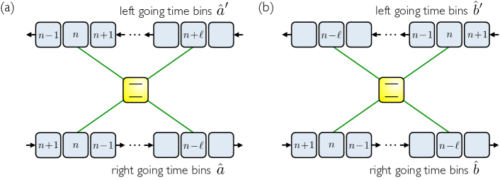
Figure 4: Alternative labeling conventions for bidirectional field time-bins. (a) The time bins interacting with the atom at the left coupling points are both labeled as “$n$”. This is the convention used in Fig.3(b). (b) In both baths, $n$ labels the two fresh time bins colliding with the system for the first time.

The atom-waveguide interaction term in the case of two coupling points is given by Eq. (Mechanism). We report it here again for the sake of clarity

$$\hat{\mathcal{H}}_{n}^{(0)}= \,\,g\,\hat{\sigma}^{\dagger}[{\hat{a}}_{n}+e^{i\varphi_{c}}e^{-i\varphi_{\text{WG}}}\,{\hat{a}}_{n-\ell}\,+\,\,{\hat{a}}_{n}^{\prime}+e^{i\varphi_{c}}e^{i\varphi_{\text{WG}}}\,{\hat{a}}_{n+\ell}^{\prime}]+{\rm H.c.}$$ (37)

Note that the primed (left-going mode) and unprimed (right-going mode) operators have different subscripts, reflecting the fact that they are traveling in opposite directions, with the same convention used in Ref. Cilluffo et al. (2020b). Equivalently, we can adopt the same labeling convention of right-going modes for left-going modes, as depicted in Fig. 4, by defining a new family of operators $\hat{b}_{m}$ such that $\hat{b}_{m}=\hat{a}_{m}$ and $\hat{b}^{\prime}_{m}=\hat{a}^{\prime}_{m+l}$. Thus we consider the couple of time-bin ladders $v=(\hat{b}_{n},\hat{b}_{n-l})$ under the condition that the first element corresponds to the right-going bath, while the second pertains to the left-going bath ($\hat{b}_{n-l}^{\prime}=\hat{a}_{n}$). It is easy to find that the composite bath operators in (Mechanism) can be generated through the action of a global transformation over $v$ as follows

$$\frac{1}{\sqrt{2}}\begin{pmatrix}1&e^{i\varphi_{c}}e^{-i\varphi_{\text{WG}}}\\ e^{i\varphi_{c}}e^{i\varphi_{\text{WG}}}&1\end{pmatrix}\begin{pmatrix}\hat{b}_{n}\\ \hat{b}_{n-l}\end{pmatrix}=\frac{1}{\sqrt{2}}\begin{pmatrix}{\hat{b}}_{n}+e^{i\varphi_{c}}e^{-i\varphi_{\text{WG}}}\,\hat{b}_{n-l}\\ e^{i\varphi_{c}}e^{i\varphi_{\text{WG}}}\,\hat{b}_{n}+\hat{b}_{n-l}\end{pmatrix}\,=\frac{1}{\sqrt{2}}\begin{pmatrix}{\hat{a}}_{n}+e^{i\varphi_{c}}e^{-i\varphi_{\text{WG}}}\,{\hat{a}}_{n-l}\\ e^{i\varphi_{c}}e^{i\varphi_{\text{WG}}}\,\hat{a}^{\prime}_{n+l}+\hat{a}^{\prime}_{n}\end{pmatrix}\,.$$ (38)

The transfer matrix is unitary if and only if $\varphi_{c}=\pi/2$ (and odd multiples). Given that the open dynamics is invariant under global unitary transformations over the environment (i.e. the waveguide), we can deduce that under this condition, the collision model where the atom interacts with the field through two points with an arbitrary delay, is equivalent to a collision model where the atom locally couples to two independent baths. Therefore the dynamics is Markovian even in the presence of arbitrarily large time delays. Note that this operation is possible because of the presence of two baths. In the context of a chiral waveguide, an extension of the bath could be identified to meet the same condition. This generally nontrivial operation exemplifies a case of Markovian embedding.

Appendix F Delay differential equation for a chiral $L$-legged giant atom

Here we show that a Markovian behavior can be obtain even with multiple coupling points, by properly tuning the coupling phases. Without loss of generality we can set $x_{1}=0$. Also, Eq. (15) is valid for any number of coupling points. Thus, we need to compute only its last term (as we did in Appendix A):

$$\sum_{k}|g_{k}|^{2}e^{i\omega_{k}(s-t)}=$$ (39)

$$= \frac{g^{2}}{N}\sum_{k}\left(L+\sum_{j=2}^{L}e^{i[\varphi_{j}+k(j-1)d]}+\sum_{j=2}^{L}e^{-i[\varphi_{j}+k(j-1)d]}+\sum_{\begin{subarray}{c}j,n=2\\ j\neq n\end{subarray}}^{L}e^{i[(\varphi_{j}-\varphi_{n})+k(j-n)d]}\right)e^{i\omega_{k}(s-t)}$$

$$= \frac{g^{2}}{N}\sum_{k}\left(L+\sum_{j=2}^{L}e^{i[\varphi_{j}+k(j-1)d]}+\sum_{j=2}^{L}e^{-i[\varphi_{j}+k(j-1)d]}+\sum_{\begin{subarray}{c}j,n=2\\ j\neq n\end{subarray}}^{L}e^{i[(\varphi_{j}-\varphi_{n})+k(j-n)d]}\right)e^{iv|k|(s-t)}$$

$$= \frac{g^{2}}{N}\sum_{k>0}\left(L+\sum_{j=2}^{L}e^{i[\varphi_{j}+(j-1)kvt_{d}]}+\sum_{j=2}^{L}e^{-i[\varphi_{j}+(j-1)kvt_{d}]}+\sum_{\begin{subarray}{c}j,n=2\\ j\neq n\end{subarray}}^{L}e^{i[(\varphi_{j}-\varphi_{n})+(j-n)kvt_{d}]}\right)e^{ivk(s-t)}$$

$$+\frac{g^{2}}{N}\sum_{k<0}\left(L+\sum_{j=2}^{L}e^{i[\varphi_{j}+(j-1)kvt_{d}]}+\sum_{j=2}^{L}e^{-i[\varphi_{j}+(j-1)kvt_{d}]}+\sum_{\begin{subarray}{c}j,n=2\\ j\neq n\end{subarray}}^{L}e^{i[(\varphi_{j}-\varphi_{n})+(j-n)kvt_{d}]}\right)e^{-ivk(s-t)}$$

$$= \frac{g^{2}}{N}\sum_{k}\left(Le^{ivk(s-t)}+\sum_{j=2}^{L}e^{i\varphi_{j}}e^{ivk[(j-1)t_{d}+s-t]}+\sum_{j=2}^{L}e^{-i\varphi_{j}}e^{-ivk[(j-1)t_{d}-s+t]}+\sum_{\begin{subarray}{c}j,n=2\\ j\neq n\end{subarray}}^{L}e^{i(\varphi_{j}-\varphi_{n})}e^{ivk[(j-n)t_{d}+s-t]}\right)+$$

$$\frac{g^{2}}{N}\sum_{k}\left(Le^{-ivk(s-t)}+\sum_{j=2}^{L}e^{i\varphi_{j}}e^{ivk[(j-1)t_{d}-s+t]}+\sum_{j=2}^{L}e^{-i\varphi_{j}}e^{-ivk[(j-1)t_{d}+s-t]}+\sum_{\begin{subarray}{c}j,n=2\\ j\neq n\end{subarray}}^{L}e^{i(\varphi_{j}-\varphi_{n})}e^{ivk[(j-n)t_{d}-s+t]}\right)$$

$$= \frac{g^{2}}{N}\sum_{k}\left(Le^{ivk(s-t)}+\sum_{j=2}^{L}e^{i\varphi_{j}}e^{ivk[(j-1)t_{d}+s-t]}+\sum_{j=2}^{L}e^{-i\varphi_{j}}e^{-ivk[(j-1)t_{d}-s+t]}+\sum_{\begin{subarray}{c}j,n=2\\ j\neq n\end{subarray}}^{L}e^{i(\varphi_{j}-\varphi_{n})}e^{ivk[(j-n)t_{d}+s-t]}\right)+$$

$$\frac{g^{2}}{N}\sum_{k}\left(Le^{ivk(s-t)}+\sum_{j=2}^{L}e^{i\varphi_{j}}e^{-ivk[(j-1)t_{d}-s+t]}+\sum_{j=2}^{L}e^{-i\varphi_{j}}e^{ivk[(j-1)t_{d}+s-t]}+\sum_{\begin{subarray}{c}j,n=2\\ j\neq n\end{subarray}}^{L}e^{i(\varphi_{j}-\varphi_{n})}e^{-ivk[(j-n)t_{d}-s+t]}\right)$$

$$= \frac{g^{2}}{N}\sum_{k}\left(2Le^{ivk(s-t)}+2\sum_{j=2}^{L}\cos(\varphi_{j})e^{ivk[(j-1)t_{d}+s-t]}+2\sum_{j=2}^{L}\cos(\varphi_{j})e^{-ivk[(j-1)t_{d}-s+t]}\right)$$

$$+\frac{g^{2}}{N}\sum_{k}\left(2\sum_{\begin{subarray}{c}j,n=2\\ j>n\end{subarray}}^{L}\cos(\varphi_{j}-\varphi_{n})e^{ivk[(j-n)t_{d}+s-t]}+2\sum_{\begin{subarray}{c}j,n=2\\ j<n\end{subarray}}^{L}\cos(\varphi_{n}-\varphi_{j})e^{-ivk[(n-j)t_{d}-s+t]}\right)$$

$$\rightarrow \frac{g^{2}}{v}\left(2L\delta(s-t)+2\sum_{j=2}^{L}\cos(\varphi_{j})\delta((j-1)t_{d}+s-t)+2\sum_{j=2}^{L}\cos(\varphi_{j})\delta((j-1)t_{d}-s+t)\right)+$$

$$\frac{g^{2}}{v}\left(2\sum_{\begin{subarray}{c}j,n=2\\ j>n\end{subarray}}^{L}\cos(\varphi_{j}-\varphi_{n})\delta((j-n)t_{d}+s-t)+2\sum_{\begin{subarray}{c}j,n=2\\ j<n\end{subarray}}^{L}\cos(\varphi_{n}-\varphi_{j})\delta((n-j)t_{d}-s+t)\right)\,.$$

Plugging back into Eq. (15) we get

$$\dot{\varepsilon}(t) = -\int_{0}^{t}\text{d}s\varepsilon(s)e^{-i\omega_{a}(s-t)}\sum_{k}|g_{k}|^{2}e^{i\omega_{k}(s-t)}$$ (40)

$$\rightarrow -\frac{g^{2}}{v}\int_{0}^{t}\text{d}s\varepsilon(s)e^{-ivk_{a}(s-t)}\times$$

$$\times\left(2L\delta(s-t)+2\sum_{j=2}^{L}\cos(\varphi_{j})\delta((j-1)t_{d}+s-t)+2\sum_{\begin{subarray}{c}j,n=2\\ j>n\end{subarray}}^{L}\cos(\varphi_{j}-\varphi_{n})\delta((j-n)t_{d}+s-t)\right)$$

$$= -\frac{g^{2}}{v}\left(L\varepsilon(t)+2\sum_{j=2}^{L}\cos(\varphi_{j})e^{ivk_{a}(j-1)t_{d}}\Theta(t-(j-1)t_{d})\varepsilon(t-(j-1)t_{d})\right)$$

$$-\frac{g^{2}}{v}\left(2\sum_{\begin{subarray}{c}j,n=2\\ j>n\end{subarray}}^{L}\cos(\varphi_{j}-\varphi_{n})e^{ivk_{a}(j-n)t_{d}}\Theta(t-(j-n)t_{d})\varepsilon(t-(j-n)t_{d})\right)$$

$$= -\frac{g^{2}}{v}\left(L\varepsilon(t)+2\sum_{j=2}^{L}\cos(\varphi_{j})e^{i(j-1)\varphi_{\text{WG}}}\Theta(t-(j-1)t_{d})\varepsilon(t-(j-1)t_{d})\right)$$

$$-\frac{g^{2}}{v}\left(2\sum_{\begin{subarray}{c}j,n=2\\ j>n\end{subarray}}^{L}\cos(\varphi_{j}-\varphi_{n})e^{i(j-n)\varphi_{\text{WG}}}\Theta(t-(j-n)t_{d})\varepsilon(t-(j-n)t_{d})\right).$$

Now with algebraic manipulation we get (we restored $\varphi_{1}$ to unify the notation, though it can still be safely set to zero)

$$\dot{\varepsilon}(t)=-\frac{g^{2}}{v}\left(L\varepsilon(t)+2\sum_{n=1}^{L-1}\left[\left(\sum_{j=1}^{L-n}\cos(\varphi_{n+j}-\varphi_{j})\right)e^{in\varphi_{\text{WG}}}\Theta(t-nt_{d})\varepsilon(t-nt_{d})\right]\right)$$ (41)

Therefore a Markovian behavior is achieved when the phases $\varphi_{2},\ldots,\varphi_{L}$ satisfy the following $L-1$ equations

$$\sum_{j=1}^{L-n}\cos(\varphi_{n+j}-\varphi_{j})=0$$ (42)

for $n=1,\ldots,L-1$.

References

- Lorenzo et al. (2013) S. Lorenzo, F. Plastina, and M. Paternostro, Phys. Rev. A 87, 022317 (2013).
- Ramos et al. (2016) T. Ramos, B. Vermersch, P. Hauke, H. Pichler, and P. Zoller, Phys. Rev. A 93, 062104 (2016).
- Haase et al. (2018) J. F. Haase, P. J. Vetter, T. Unden, A. Smirne, J. Rosskopf, B. Naydenov, A. Stacey, F. Jelezko, M. B. Plenio, and S. F. Huelga, Phys. Rev. Lett. 121, 060401 (2018).
- Fang et al. (2018) Y.-L. L. Fang, F. Ciccarello, and H. U. Baranger, New Journal of Physics 20, 043035 (2018).
- Milz et al. (2020) S. Milz, D. Egloff, P. Taranto, T. Theurer, M. B. Plenio, A. Smirne, and S. F. Huelga, Phys. Rev. X 10, 041049 (2020).
- White et al. (2020) G. A. L. White, C. D. Hill, F. A. Pollock, L. C. L. Hollenberg, and K. Modi, Nature Communications 11, 6301 (2020).
- Tserkis et al. (2023) S. Tserkis, K. Head-Marsden, and P. Narang, “Information back-flow in quantum non-markovian dynamics and its connection to teleportation,” (2023), arXiv:2203.00668 [quant-ph] .
- Kannan et al. (2020) B. Kannan, M. J. Ruckriegel, D. L. Campbell, A. Frisk Kockum, J. Braumüller, D. K. Kim, M. Kjaergaard, P. Krantz, A. Melville, B. M. Niedzielski, A. Vepsäläinen, R. Winik, J. L. Yoder, F. Nori, T. P. Orlando, S. Gustavsson, and W. D. Oliver, Nature 583, 775 (2020).
- Frisk Kockum (2020) A. Frisk Kockum, “Quantum optics with giant atoms—the first five years,” in Mathematics for Industry (Springer Singapore, 2020) p. 125–146.
- Cilluffo et al. (2020a) D. Cilluffo, A. Carollo, S. Lorenzo, J. A. Gross, G. M. Palma, and F. Ciccarello, Phys. Rev. Res. 2, 043070 (2020a).
- Leonforte et al. (2024) L. Leonforte, X. Sun, D. Valenti, B. Spagnolo, F. Illuminati, A. Carollo, and F. Ciccarello, “Quantum optics with giant atoms in a structured photonic bath,” (2024), arXiv:2402.10275 [quant-ph] .
- Andersson et al. (2019) G. Andersson, B. Suri, L. Guo, T. Aref, and P. Delsing, Nature Physics 15, 1123 (2019).
- Tufarelli et al. (2013) T. Tufarelli, F. Ciccarello, and M. S. Kim, Phys. Rev. A 87, 013820 (2013).
- Tufarelli et al. (2014) T. Tufarelli, M. S. Kim, and F. Ciccarello, Phys. Rev. A 90, 012113 (2014).
- González-Tudela and Cirac (2017) A. González-Tudela and J. I. Cirac, Phys. Rev. A 96, 043811 (2017).
- Kockum et al. (2018) A. F. Kockum, G. Johansson, and F. Nori, Phys. Rev. Lett. 120, 140404 (2018).
- Carollo et al. (2020a) A. Carollo, D. Cilluffo, and F. Ciccarello, Phys. Rev. Res. 2, 043184 (2020a).
- Lodahl et al. (2017) P. Lodahl, S. Mahmoodian, S. Stobbe, A. Rauschenbeutel, P. Schneeweiss, J. Volz, H. Pichler, and P. Zoller, Nature 541, 473 (2017).
- Joshi et al. (2023) C. Joshi, F. Yang, and M. Mirhosseini, Phys. Rev. X 13, 021039 (2023).
- Shen and Fan (2009) J.-T. Shen and S. Fan, Phys. Rev. A 79, 023837 (2009).
- Kim et al. (2021) E. Kim, X. Zhang, V. S. Ferreira, J. Banker, J. K. Iverson, A. Sipahigil, M. Bello, A. González-Tudela, M. Mirhosseini, and O. Painter, Phys. Rev. X 11, 011015 (2021).
- Scigliuzzo et al. (2022) M. Scigliuzzo, G. Calajò, F. Ciccarello, D. Perez Lozano, A. Bengtsson, P. Scarlino, A. Wallraff, D. Chang, P. Delsing, and S. Gasparinetti, Phys. Rev. X 12, 031036 (2022).
- Zhang et al. (2023) X. Zhang, E. Kim, D. K. Mark, S. Choi, and O. Painter, Science 379, 278 (2023).
- Ciccarello et al. (2022) F. Ciccarello, S. Lorenzo, V. Giovannetti, and G. M. Palma, Physics Reports Quantum collision models: Open system dynamics from repeated interactions, 954, 1 (2022).
- Ciccarello (2018) F. Ciccarello, Quantum Measurements and Quantum Metrology 4 (2018), 10.1515/qmetro-2017-0007.
- Cilluffo et al. (2020b) D. Cilluffo, A. Carollo, S. Lorenzo, J. A. Gross, G. M. Palma, and F. Ciccarello, Phys. Rev. Res. 2, 043070 (2020b).
- Hsu et al. (2016) C. W. Hsu, B. Zhen, A. D. Stone, J. D. Joannopoulos, and M. Soljačić, Nature Reviews Materials 1, 16048 (2016).
- Calajó et al. (2019) G. Calajó, Y.-L. L. Fang, H. U. Baranger, and F. Ciccarello, Phys. Rev. Lett. 122, 073601 (2019).
- Carollo et al. (2020b) A. Carollo, D. Cilluffo, and F. Ciccarello, Phys. Rev. Res. 2, 043184 (2020b).
- Magnus (1954) W. Magnus, Communications on pure and applied mathematics 7, 649 (1954).
- Loudon (2000) R. Loudon, The quantum theory of light (OUP Oxford, 2000).
- Breuer and Petruccione (2007) H.-P. Breuer and F. Petruccione, The Theory of Open Quantum Systems (Oxford University Press, Oxford, 2007).