1
Homeostatic motion planning with innate physics knowledge
Lafratta, G.1
Porr, B.1
Chandler, C.2
Miller, A.2
1School of Engineering, University of Glasgow
2School of Computing Science, University of Glasgow.
Keywords: Planning, homeostasis, closed loop, autonomous agents
Abstract
Living organisms interact with their surroundings in a closed-loop fashion, where sensory inputs dictate the initiation and termination of behaviours. Even simple animals are able to develop and execute complex plans, which has not yet been replicated in robotics using pure closed-loop input control. We propose a solution to this problem by defining a set of discrete and temporary closed-loop controllers, called “tasks”, each representing a closed-loop behaviour. We further introduce a supervisory module which has an innate understanding of physics and causality, through which it can simulate the execution of task sequences over time and store the results in a model of the environment. On the basis of this model, plans can be made by chaining temporary closed-loop controllers. The proposed framework was implemented for a real robot and tested in two scenarios as proof of concept.
1 Introduction
Living organisms interact with their surroundings through sensory inputs in a closed-loop fashion (Maturana and Varela, 1980; Porr and Wörgötter, 2005). To recreate closed-loop navigation in a robot it is sufficient to directly connect a robot’s sensors to its motor effectors, and the specific excitatory or inhibitory connections determine the control strategy, as detailed in Braitenberg (1986). These sensor-effector connections represent a single closed-loop controller, which produces stereotyped behaviour in response to an immediate stimulus. For this reason, closed-loop control by itself is not suitable to formulate complex navigation plans.
A wide variety of techniques have been developed over the years to achieve safe spatial navigation in complex scenarios. These can be learning-based, reactive, or a combination of the two. Reinforcement Learning (RL) is possibly the most popular learning-based paradigm. In RL, an agent learns to associate actions with specific inputs or ”states” through repeated interactions with the environment, aiming to maximise the cumulative reward (Sun et al., 2021). Rewards represent feedback for the action taken, making for a closed-loop output control paradigm. RL has been very successful in recent years, when supplemented with techniques such as deep learning (Mnih et al., 2015; Silver et al., 2016; OpenAI, 2023). RL models are inherently slow to train for two main reasons. Firstly, rewards are sparse. Secondly, in output control, feedback about the action can only be obtained after the action has been completed; the action will therefore be corrected in the next training episode. Contrast this with input control, where feedback on the action is continuously provided by sensors and motor outputs can be corrected immediately. The outputs of a naive RL model are therefore typically associated with high error and/or low reward (cfr. benchmarks in Thodoroff et al. 2022). For example, Mila and Pal (2019) developed a Real-Time Actor-Critic paradigm which, despite being able to achieve faster convergence than the classical Soft Actor-Critic one, still required hundreds of thousands of training steps, which could take hours or days to complete (Dalton and Frosio, 2020). As a consequence, the training of RL models typically occurs offline. To this day, fully online RL remains unfeasible, with the consequence that an automated agent is not able to acquire knowledge tailored to its own environment in real-time. Instead, large models must be trained in order for a system to be able to generalise to a variety of unseen scenarios. This is not only computationally expensive, but also compromises the transparency of the model learned, especially if very large and/or trained on cloud platforms (Vasudevan et al., 2021).
Reactive algorithms, on the other hand, simply generate trajectories for a robot to follow based on the position of obstacles or targets in the environment without requiring any training. Trajectories are usually calculated based on nodes in a graph, randomly generated (see Karur et al., 2021 for an in-depth review), or tailored to sensory inputs using force fields (e.g. Vector Field Histogram (Borenstein and Koren, 1991) or Artificial Potential Fields (Khatib, 1985)). From a control theory perspective, trajectories can be viewed as a series of desired inputs for a single controller, representing the desired locations of a robot in a global frame of reference. Loop closure in this case consists of providing feedback on how closely the robot follows its trajectory. Trajectory following is a form of input control; however, feedback input is usually provided by an external observer (e.g. a camera placed on the ceiling), as a robot is oblivious to its own objective trajectory. Contrast this with a Braitenberg vehicle, which only needs information about the location of a disturbance (e.g. obstacle or target) relative to itself to successfully perform a control action.
Like in RL, motor plans for robots should consist of sequences of actions, taken in response to inputs. However, in even simple animals like the common fruit fly, complex plans in unknown environments can be formulated completely on-the-fly (Honkanen et al., 2019). This challenges the notion that learning through trial and error is necessary at all for planning. In Spelke and Kinzler (2007) the concept of “core knowledge” is introduced. This is intended as a seemingly innate understanding of basic properties of one’s environment such as physics and causality, and is backed by studies on newborn animals. An agent equipped with core knowledge can form reasonable predictions over the outcome of an action without needing to perform it, which benefits the efficiency of the decision making process. A contribution in the direction of providing a system with innate knowledge has been attempted in few-shot RL. In this paradigm, the goal is for a system to be able to choose and adapt policies to unseen scenarios with just a few training examples. This is achieved by using meta-learning (Luo et al., 2021; Bing et al., 2023) or transfer-learning (Sun et al., 2023) algorithms, or both (Shu et al., 2023) which, in brief, use previously trained RL models as a foundation for a novel model to be trained. While able to outperform pure RL in terms of training time, both the preexisting and the novel models are trained offline, suggesting that the response time of few-shot learning may still be unsuitable for real-time training.
Our research addresses the problems of how to achieve multi-step-ahead planning using closed-loop control, and of how to implement core knowledge in an agent as a tool to aid decision-making. To tackle the first problem, we define various control loops, which we will call “tasks”, each representing a distinct control strategy. For example, we may have a loop which only counteracts obstacles by turning left, or one that only turns right, etc. Control loops are contingent to specific sensory inputs that make them necessary (Porr and Wörgötter, 2005). They are therefore temporary and can be chained sequentially in a variety of combinations. As for the second problem, we introduce core knowledge (Spelke and Kinzler, 2007) as a simulation which runs in parallel to and mirrors the real world. This allows us to simulate sequences of tasks representing potential plans. Our framework, therefore, is characterised by the the concurrent operation of temporary closed-loop controllers both physically and in simulation. This setup necessitates an overarching supervising module (Porr and Wörgötter, 2005) which oversees the task creation process. This module, which we will call “Configurator” (cfr. LeCun (2022)) directs the simulation, interprets its results to formulate a plan, and executes plans by creating and terminating tasks accordingly. Crucially, both task execution and planning are formulated as homeostatic control problems: in the former, motor outputs are generated in order to counteract sensory stimuli which pose a disturbances to a desired state, and in the latter, a plan is chosen which maximises the time spent in that state.
The paper is organised as follows. In Section 2.2 we describe in detail the components of the proposed framework; in Section 2.3 we discuss the features of our specific implementation; in Section 3 we present the results of the experimental validation of the framework; in Section 4 we discuss the results in light of the state of the art.
2 Methods
2.1 Overview of proposed approach
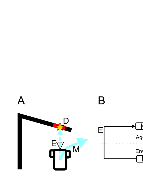
In Figure 1A we present an informal definition of a task. A task begins when a disturbance (in this case obstacle ) enters the robot’s sensor range. The sensors produce a signal which is relayed directly to the motor effectors which produce reflex motor output . A task executes until the disturbance ceases to produce a signal, at which point the task simply terminates. When no disturbance is present, the system falls back on a “default” task which characterises the resting state. Importantly, unlike in classical closed-loop control, where the control problem is tackled by a single controller at all times, each task is discarded upon termination and may be replaced by any other task.

Figure 2 provides an overview of how tasks and core knowledge can be combined to generate plans in the form of task sequences. Tasks are denoted with letter , core knowledge is depicted as a thought balloon (Figure 2A-B), and the Configurator is represented in Figure 2C. The “default” behaviour is in this case arbitrarily defined as driving straight.
In the beginning, the Configurator is executing an initial task , depicted in Figure 2D-E, where a robot by default drives straight ahead (this task type is denoted by ) with no disturbance to counteract (). Figure 2A represents the use by the Configurator of core knowledge to simulate tasks ahead of the present: the simulation results represent the scenarios likely to arise from the execution of the sequence. These scenarios, comprised of tasks and the disturbances encountered as a result of executing them, can be collected in a searchable structure, as depicted in Figure 2B. Nodes in this structure are denoted as , and they each contain a task and any disturbance (denoted as a star) encountered in its simulation .
The initial task is represented in Figure 2B in node , and from it stem three task sequences. First, default task is created: through its simulation (Figure 2A), the Configurator finds that the robot will collide with obstacle (depicted as a star) represented by the wall in front. Task is in node in Figure 2B. The second control strategy is a left turn (denoted with type ) represented by task , which executes successfully in simulation. Task is followed by default task , which ends in a collision. This sequence can be observed in Figure 2B as nodes . Lastly, the Configurator explores a third strategy of following with task , a right turn (denoted with type ). executes without disturbances and is followed by default task . These tasks are nodes in Figure 2B.
The process of finding a plan involves a search over the structure in Figure 2B. In our case, this search produces the disturbance-free sequence , (indicated by thick arrows in Figure 2B), which will be queued for execution. The execution is shown in Figures 2F-G: initial task has been overwritten as a task of type , constructed to counteract the obstacle . As predicted, no disturbances are found to arise during its execution (the simulation is omitted): as in Figures 2H-I, when ends, it is again overwritten as another default task , initialised with a void disturbance .
2.2 Theoretical foundations
2.2.1 Tasks as closed-loop controllers
Formally, we define tasks as closed-loop controllers, as depicted in Figure 1B. Tasks are contingent to a disturbance which enters the Environment transfer function , and generates an error signal . This signal is used by the Agent (i.e. the robot) transfer function to generate a motor output aimed at counteracting the disturbance (e.g. avoiding the obstacle in Figure 1A). Once the disturbance is counteracted, the error signal becomes zero: at this point, the control motor output is no longer needed and the execution of the control loop terminates.
We define three discrete types of tasks representing the behaviours of driving straight ahead (), turning left (), and turning right (), and we call the corresponding outputs , respectively. Of these, we arbitrarily set tasks as the “default” (see Section 1) behaviour, so that in a disturbance-free scenario the robot just drives straight ahead. Further, we allow our robot to exhibit obstacle avoidance and target pursuit. We therefore divide disturbances between obstacles and targets by assigning them, respectively, a label through the function .
2.2.2 Hybrid control
The simulated task-chaining process has a discrete domain i.e. the task which is being simulated, and a continuous one, i.e. the evolution of sensory inputs over time during task simulation. For this reason, the rules underlying task simulation can be summarised using a nondeterministic hybrid automaton (Henzinger, 2000; Raskin, 2005; Lafferriere et al., 1999).
A hybrid automaton is a tuple , where
-
•
T is a finite set of control modes, or the discrete states of the system.
-
•
is a set of variables representing the continuous state of the system. We use to represent the derivatives of , or the evolution of the continuous variables over time, and “primed” variables to denote the valuation of with which the next control mode is initialised.
-
•
represents the edges, or permitted transitions between control modes
-
•
are functions assigning each a predicate to each control mode.
is the flow function. defines the possible continuous evolutions of the system in control mode .
is the invariant function. represents the possible valuations for variables in control mode .
-
•
are functions which assign a predicate to each edge.
is the jump function. is a guard which determines when the discrete control mode change represented by edge is allowed based on the valuation of the continuous component .
is the reset function. assigns to edge possible updates for the variables when a discrete change occurs. This is represented by an assignment to primed variables .
In our implementation (discussed in more depth in Section 2.3), the discrete “control modes” are tasks and the continuous variables are sensory inputs. The flow functions are the velocities corresponding to task-specific motor outputs, the invariant predicates define inputs to which each task is contingent, the jump guards set conditions which must be met by the continuous inputs for a transition along a certain edge, and resets assign values to the continuous variables which will determine the initial inputs at the start of a certain task.
The unfolding over time of a hybrid automaton can be represented as a transition system , where is a set of states, and is a transition relation corresponding to edges connecting states. This transition system represents a model of the environment constructed through simulated interaction. We denote
| (1) |
| (2) |
Further, we define a path where , where is the root state in the transition system. Paths represent sequences that may potentially constitute a plan.
2.2.3 The Configurator as a supervisor
We define the Configurator as a type of supervisor (Ramadge and Wonham, 1984):
| (3) |
where is a hybrid automaton as described in Section 2.2.2, is the system’s overarching goal, or the disturbance which the plan aims to counteract, is an “explorer” function which generates transition system representing possible runs of , and is a “planner” function which extracts a goal-directed path from a transition system.
2.3 Implementation
2.3.1 Robot
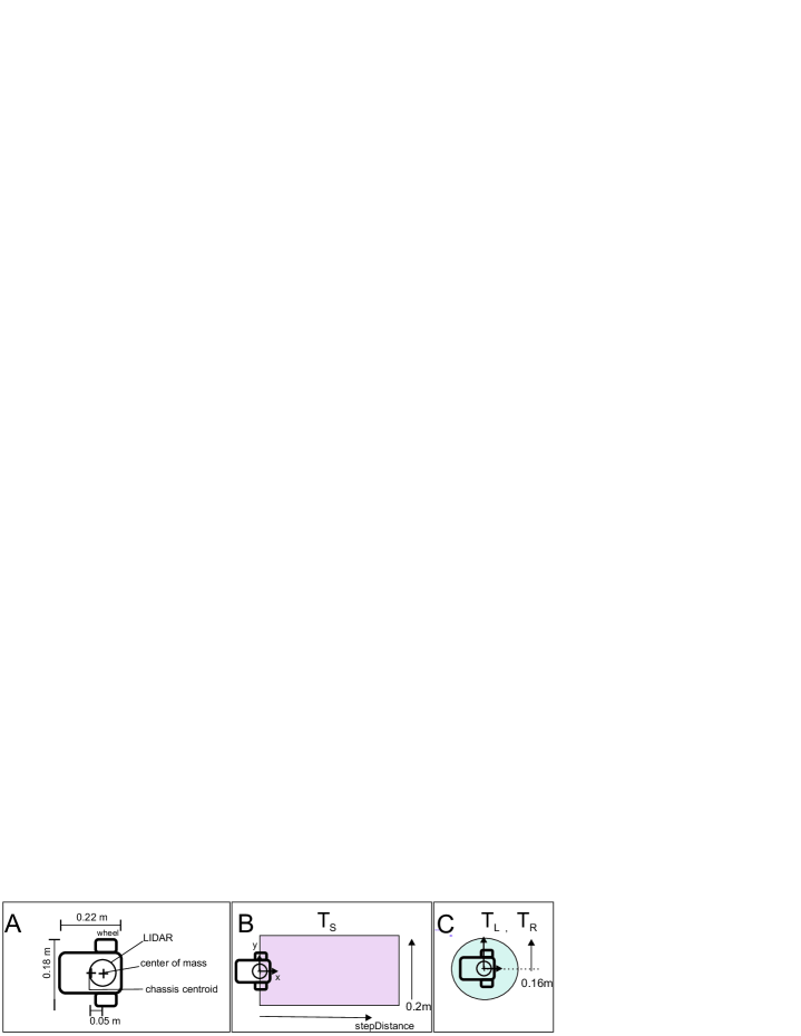
We implement the outlined framework on an indoor robot based on the Alphabot111https://www.waveshare.com/alphabot-robot.htm (see Figure 3A). The robot is equipped with a Rasbperry Pi Model 3b+ (Broadcom BCM2837B0 processor with a 1.4 GHz clock speed and 1 GB RAM), an A1 Slamtec 2D LIDAR sensor and two 360o continuous rotation servos which move the wheels. The LIDAR callback runs at 5 Hz and the motors are updated at 10 Hz. We define the motor update as .
2.3.2 Core knowledge as a physics simulation
We represent core knowledge as simulation in the physics engine Box2D222https://box2d.org/ where the coordinates represents the robot’s local frame of reference. All data pertaining to position and its derivatives are expressed as 2D transforms of the form , where represents the position in Cartesian coordinates in meters and is the orientation in radians of the object. Obstacles in Box2D are objects of dimensions 0.001m x 0.001m located at coordinates extracted from LiDAR input. The robot was modelled as a simple rectangle of dimensions 0.22m 0.18m on the local x and y axis, respectively, with the center of mass shifted forward on the local x axis by 0.05m (see Figure 3A).
The physics simulation may progress for an arbitrarily long (simulated) time, and the world and its content are updated with each arbitrarily small time step . Simulated sensors can be added to objects which report collisions between objects. Task simulation is interrupted as soon as a collision is reported, and the first point of contact between fixtures is returned as the disturbance.
We limit the range of the sensor data used for the simulation to m from the origin. This represents a planning horizon, and the simulation stops when its limit is reached. The simulation is advanced using a kinematic model of the robot with a time step (), 3 position iterations, 8 velocity iterations so that a simulation carries on for a variable number of steps, indicated as .
The speed of the Box2D simulation is sensitive to the number of simulated objects: to reduce computational demands, we perform some simple filtering on the LiDAR coordinates as depicted in Figure 3B-C. For simulating tasks of type , we only represent points located within a distance from the robot’s center of mass, where denotes a finite distance range in meters for that task type. For left and right turns and in Figure 3C we only retain points located within a radius of 0.16m from the robot’s center of mass. The filtered data thus obtained is further filtered using one of the following techniques. The first technique, “worldbuilding1”, consists of approximating each coordinate to two decimal places and eliminating redundant value. For the second, “worldbuilding2”, only every other point in the set constructed using “worldbuilding1” is retained.
Simulation results can be used to determine motor commands for task execution in the real world. We calculate each motor command as a duration expressed as a number of motor update intervals
| (4) |
where is the number of steps of size taken to bring a task to termination in simulation and calculates the simulated time which the task has taken.
2.3.3 Hybrid automaton
The hybrid automaton modelling the simulated task-switching process is depicted in Figure 4.
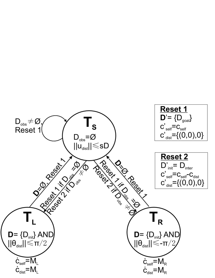
The discrete control modes corresponding to tasks , are inscribed in circles connected by arrows representing the edges . Continuous variables correspond to sensor inputs in the form of 2D transforms. These inputs are: the position of the robot , the change in the robot’s position since the start of the task , and disturbance set , comprised of the disturbance to which the task is contingent , and the disturbance interrupting task execution . Flow predicates are annotated outside of each circle. Invariant predicates are annotated inside each circle. Jump and reset predicates are located by the corresponding edges.
Task models the behaviour of the system when it is driving straight, while tasks and model the behaviours of turning left and right, respectively. As indicated by the respective flow predicates, the position of the robot and the position change since the start of the task evolve at a rate denoted by task-specific velocities for driving stright, for left turns, and for right turns, all in local coordinates. These values were calculated applying simple robot kinematics to empirical velocity measurements.
As indicated by the corresponding invariant predicate, task executes as long as no obstacles (defined as ) are present and the robot has not yet covered a fixed distance (abbreviated to in Figure). As indicated by the respective invariant predicates, tasks and keep executing as long as the only disturbance in the continuous variables is the one on which the task is contingent (predicate ), and the angle described by the turn has not yet reached rad (for task ), and rad for task . Note that these invariant predicates still allow for a turn to execute in the case a task may be initialised with an empty disturbance.
Transitions along edge are permitted if the terminated task has not encountered obstacles, as indicated by jump predicate . Transitions along edges and , are permitted if the left or right turns are terminated with no disturbances, as indicated by jump predicates . Transitions along edges and are always permitted, as indicated by the lack of jump guards.
The boxes on the right-hand side of Figure 4 contain the two reset predicates, “Reset1” and “Reset2”, which assign to primed variables depending on whether the most recently simulated task is terminated without disturbances, or if it encounters an obstacle, respectively. For all reset predicates, every time the system switches control mode, the distance covered in the previous task is reset to a zero transform . The “Reset1” predicate states that the next task will start where the previous one ended () and will be aimed at reaching the goal ( ). The “Reset2” predicate states that the next task will be primed to counteract the obstacle () which interrupted the previous task, and it will start where the previous task began (). “Reset1” always applies to edges , and to edges and if the continuous state does not contain obstacles (). If obstacles are present () in these last two edges, “Reset2” applies.
2.3.4 The explorer
The explorer uses a best-first approach to construct transition system from automaton . The priority of expansion of a state is defined by its cumulative past and expected cost (cfr. Hart et al. 1968), which we will define as function . Additionally, we use a heuristic function to prevent the robot from turning more than 180 degrees on the spot and getting stuck rotating in place.
We calculate cost evaluation function as:
| (5) |
where are states in transition system , calculates the past cost associated with state and is a heuristic function which estimates the cost to reach goal from state .
We define the past cost function as:
| (6) |
where is a disturbance encountered in state , represents the maximum possible distance that the robot can be from a disturbance, and represents the Euclidean distance between task start position (see Section 2.2.2) and disturbance .
We define the cost heuristic function:
| (7) |
where represents the distance between the robot’s position at the end of the simulation of state and target . We further define heuristic function as:
| (8) |
where 2D transforms and represent the robot’s position and orientation at the end of the simulation of state and , respectively.
Algorithm 1 provides pseudocode for explorer . We start from a transition system and priority queue , where is a starting state representing the task being executed by the robot. The corresponding task is immediately terminated, in order for the system to explore the scenarios that would arise if the robot were to change its behaviour immediately, without waiting for the task at state to terminate.
We use to denote the state with the lowest evaluation in the priority queue; its out-edges are explored with the highest priority. We further denote the state whose out-edges are actively being explored with and the frontier state with . Any permitted transitions from state are explored in a depth-first fashion until frontier state contains a task (zero to two states ahead of state ). After the expansion of is complete, is reset to the node which has the smallest value in the priority queue, and the process repeats until a path is found which leads to a goal or the planning horizon. Note how this implies that only tasks of the type are evaluated and that is, therefore, always a task .
2.3.5 Planner
The model generated by the explorer is used by planner defined in Section 3, which returns a path which brings the robot as close to the goal as possible. Formally we write:
| (9) |
3 Results
We test the decision-making process by applying it to two real-world problems: one of avoiding of being trapped in a cul-de-sac and one of simultaneous collision avoidance and target pursuit. We contrast our new approach against a Braitenberg-style control strategy which uses a single closed-loop controller and therefore exhibits stereotyped behaviour.
Sequences of tasks and the specifications of the motor commands pertaining to each task are planned at the beginning of the experimental task and do not undergo correction throughout execution. The amount of time taken by the robot to formulate a plan is measured, as well as the total amount of objects simulated in Box2D and the number of states in the transition system, which are equivalent to the number of tasks simulated.
3.1 Experiment 1: cul-de-sac avoidance
Our first experiment tests our approach in a cul-de-sac avoidance scenario. This is a classical scenario where reactive behaviour is not sufficient to prevent getting stuck in a cul-de-sac. We set and m. The experiment was repeated six times with “worldbuilding1”, and twelve with “worldbuilding2”.
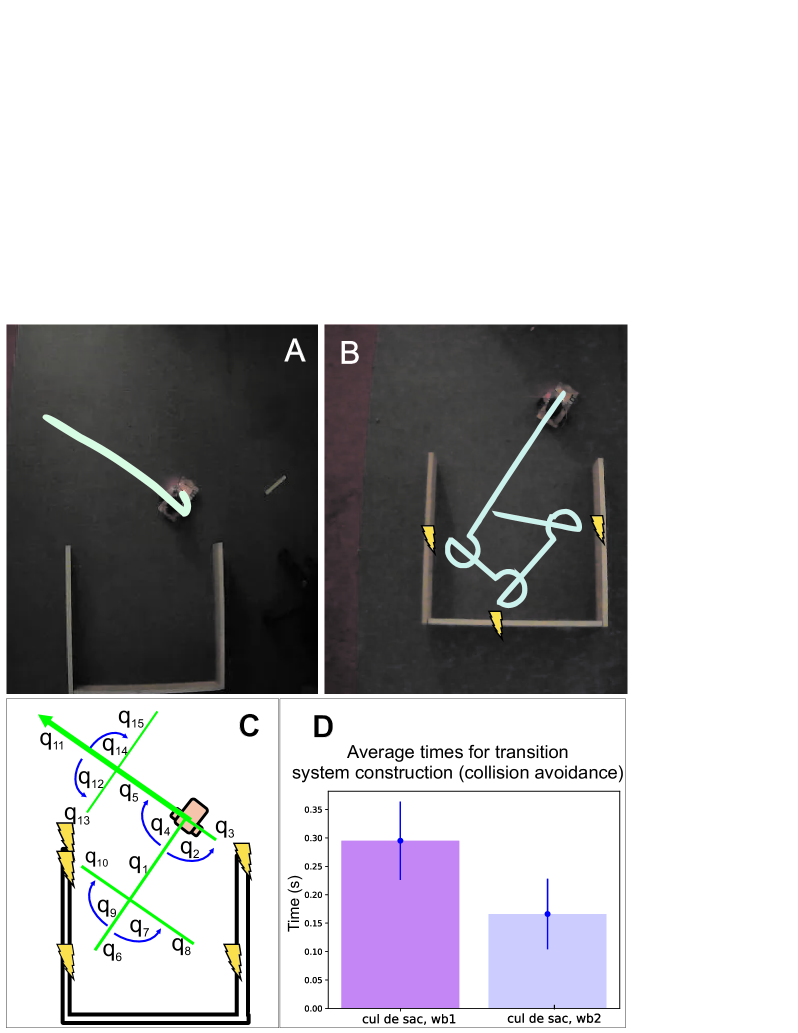
Figure 5 depicts a comparison of the behaviour planned using our new multiple-loop framework (Figure 5A), and the single-loop reactive behavioural case (Figure 5B), and the reasoning process employed using our framework (Figure 5C). As can be observed from the trance in Figure 5A, when the robot uses our multi-step-ahead planning strategy, it identifies the cul-de-sac immediately and, to prevent entering it, turns to its right which allows it to carry on undisturbed. By contrast, in the single-loop control experiment, the robot enters the cul-de-sac, as it is outside of the single loop’s range . Moreover, as signified in yellow lightning, some collisions occur during execution.
Figure 5C offers a visual representation of the construction of transition system constructed in one of the experimental runs and the plan extracted from it. Initial state is immediately terminated and from its end position (see robot schematic in Figure 5C), transition system building starts. The robot may safely proceed straight (state ) or turn right and then advance (states ). The sequence cannot be safely executed since, in state , the robot collides with the wall ahead of it. States and will have the same value and rank higher in the priority queue than state .
The cul-de-sac is discovered as all the sequences following state (namely, state , states and states . State will now therefore have highest priority, and will be expanded. Three other state sequences are added to this node. Of these, driving right and straight (states ) leads to a crash, while state and sequence are disturbance-free. In this case, state reaches the limit of the planning horizon before state , for which reason planning can end. The final plan, indicated by the bold arrow in Figure 5C, is , where , , , .
Figure 5D displays the descriptive statistics pertaining to simulation and planning speed. In runs where worldbuilding1 was used to create objects in the Box2D environment (in Figure, column labelled ”cul-de-sac, wb1”), an average of 19.3 states (min: 16, max: 26) were simulated with 93.8 average total objects (SD=39.93) created over the course of the simulation. This took on average 0.295s (SD=0.069s). With worldbuilding2 (in Figure, column labelled ”cul-de-sac, wb2”), an average of 20.16 states (min: 11, max: 21) were simulated with 40.75 average total objects (SD=20.67) in 0.166s on average (SD= 0.062s).
3.2 Experiment 2: avoidance and target behaviour
Figure 6 represents the results of an experiment where the robot had to reach a target while driving around an obstacle. We set corresponding to the diameter of the robot, as in (Ulrich and Borenstein, 2000). The experiment was repeated ten times with “worldbuilding1”, and eight with “worldbuilding2”.
As shown in Figure 6B, in the reactive behaviour experiment the robot remains stuck behind the obstacle, while in our approach (Figure 6A) the agent is able to safely formulate a plan to reach the target.
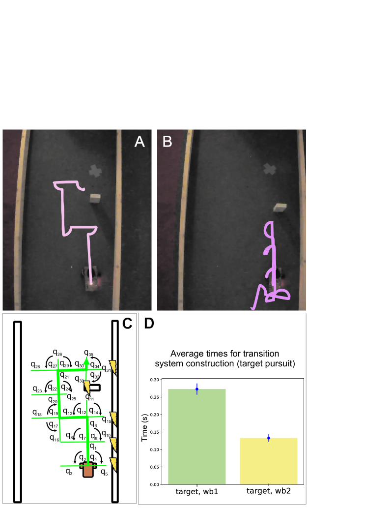
Figure 6C depicts the transition system produced in one of the experimental runs. As shown, the robot can safely advance towards the target by entering states . Further advancement through state is prevented by an obstacle. The only collision-free option for the robot is to turn left (state ) and proceed in a direction perpendicular to the target (state ). The robot will then turn towards the disturbance by choosing to turn right (state ) and then proceed straight (). The robot will then immediately attempt to return in line with the target by turning left and then proceeding straight (states ), but these options are not collision-free. By transitioning to state , the robot will drive straight towards the target; after this, it may safely turn right (state ) and return in line with the target (state ). The target is now very close: by turning left (state ), the robot positions itself to face it and advances (state ) until it reaches it, at which point transition system construction terminates. As indicated by the bold arrow in Figure 6C, the plan followed in Figure 6A is , where , , , , , , , , , , .
Descriptive statistics for the simulation and planning speed are shown in Figure 6D. Using worldbuilding1 (in Figure, column labelled ”target, wb1”), the transition system was made up of an average of 37.8 states (min: 36, max: 39), and each simulation contained on average 114.4 objects (SD=21.08). The mean simulation time was 0.273s (SD= 0.016s). When worldbuilding2 (in Figure, column labelled ”target, wb2”) was employed, the mean number of states was similar at 38.25 with the same minimum and maximum values. The average number of objects was reduced to 64.38 (SD=11.70), and average simulation time dropped to 0.133s (SD=0.011s).
4 Discussion
In this paper we have introduced a novel decision-making process which exploits supervisory control of a hybrid automaton representing temporary simulated closed-loop controllers, called “tasks”, representing each a different control strategy. The simulation of the task-switching process occurs in a physics engine which constitutes the system’s core knowledge. The performance of the decision-making process was tested in a real robot in a collision avoidance problem and a target pursuit one. The robot was in both cases able to generate, in real-time, a model of tasks and their resulting disturbances over a 1m range, which was used to extract a plan. We contrasted this performance with a classical closed-loop system where planning can only occur one disturbance into the future and the system behaves deterministically. This control case produced less efficient behaviour in the best case scenario and failed by colliding with a wall or remaining stuck in the worst.
We construct a model of the environment as a hybrid transition system representing possible runs of a hybrid automaton. Problems concerned with the combination of discrete and hybrid control are referred to as Task And Motion Problems (TAMP). TAMPs are notoriously difficult to solve in real-time: in recent years neural networks have been used to train complex models aimed at combining planning over a hybrid transition system and learning control policies in a variety of scenarios (Kim et al., 2022; Driess et al., 2021). This obviously requires offline training and has potential for limited transparency and/or robustness depending on the depth of the network used. Additionally, even with previous training, planning times in Kim et al. (2022) fell into the order of hundreds of seconds; this is not suitable for real-world applications.
Online approaches to hybrid control for navigation have also been proposed. In Mavridis et al. (2019); Constantinou and Loizou (2018); Migimatsu and Bohg (2020), hybrid automata are constructed using various types of logic to check that they satisfy certain properties. Whether the control modes may be immediately available to the system (Migimatsu and Bohg, 2020) or may need to be computed (Mavridis et al., 2019), the computation of the control-mode-specific flow function can be an inefficient process. Computation statistics were not reported in Mavridis et al. (2019); Constantinou and Loizou (2018), however Migimatsu and Bohg (2020) report that the minimum time taken for convergence to an optimal continuous control was 0.85 seconds. A model-checking approach was proposed by Chandler et al. (2023) over a discrete-state system, which was able to plan over a sequence of five actions in around 0.01s. This suggests that the optimisation over continuous controls may be the bottleneck for TAMP problems.
While we do not focus on achieving smooth trajectories or more complex tasks such as grasping, we were able to achieve planning in real-time or near-real-time in a robot with very limited computational power. The closed-loop task simulation allowed us to easily obtain an estimation of the commands for the motor effectors. Starting from a reasonable estimation of a control output may relieve some of the computational load resulting from its optimisation, which should occur online and in a closed-loop fashion. Despite the increased planning time in our experiments compared to Chandler et al. (2023), the speed performance recorded in our experiments is still within human reaction time range (Wong et al., 2015) and within real-time requirements of the robot.
In conclusion, our findings demonstrate that not only it is possible to formulate optimal plans based on pure input control, but it is also achievable in real-time over the discrete and continuous domains, thanks to core knowledge. We believe that our framework has potential to scale well to TAMP problems, in at least two dimensions, and provide a valuable complement to the state-of-the-art.
5 Acknowledgements
This work was supported by a grant from the UKRI Engineering and Physical Sciences Research Council Doctoral Training Partnership award [EP/T517896/1-312561-05]; the UKRI Strategic Priorities Fund to the UKRI Research Node on Trustworthy Autonomous Systems Governance and Regulation [EP/V026607/1, 2020-2024]; and the UKRI Centre for Doctoral Training in Socially Intelligent Artificial Agents [EP/S02266X/1].
References
- Bing et al. (2023) Zhenshan Bing, David Lerch, Kai Huang, and Alois Knoll. Meta-reinforcement learning in non-stationary and dynamic environments. IEEE Transactions on Pattern Analysis and Machine Intelligence, 45:3476–3491, 3 2023. ISSN 19393539. doi: 10.1109/TPAMI.2022.3185549.
- Borenstein and Koren (1991) Johann Borenstein and Yoram Koren. The vector field histogram—fast obstacle avoidance for mobile robots. IEEE Transactions on Robotics and Automation, 7:278–288, 1991. doi: 10.1109/70.88137.
- Braitenberg (1986) V. Braitenberg. Vehicles: Experiments in Synthetic Psychology. MIT Press, 1986.
- Chandler et al. (2023) Christopher Chandler, Bernd Porr, Alice Miller, and Giulia Lafratta. Model checking for closed-loop robot reactive planning. Electronic Proceedings in Theoretical Computer Science, 395:77–94, 11 2023. doi: 10.4204/EPTCS.395.6.
- Constantinou and Loizou (2018) Christos C. Constantinou and Savvas G. Loizou. Automatic controller synthesis of motion-tasks with real-time objectives. Proceedings of the IEEE Conference on Decision and Control, 2018-December:403–408, 7 2018. doi: 10.1109/CDC.2018.8619825.
- Dalton and Frosio (2020) Steven Dalton and Iuri Frosio. Accelerating reinforcement learning through gpu atari emulation. Advances in Neural Information Processing, 33:19773–19782, 2020.
- Driess et al. (2021) Danny Driess, Jung Su Ha, and Marc Toussaint. Learning to solve sequential physical reasoning problems from a scene image. International Journal of Robotics Research, 40:1435–1466, 12 2021. ISSN 17413176. doi: 0.1177/02783649211056967.
- Hart et al. (1968) Peter E. Hart, Nils J. Nilsson, and Bertram Raphael. A formal basis for the heuristic determination of minimum cost paths. IEEE Transactions on Systems Science and Cybernetics, 4:100–107, 1968. ISSN 21682887. doi: 10.1109/TSSC.1968.300136.
- Henzinger (2000) Thomas A. Henzinger. The theory of hybrid automata. Verification of Digital and Hybrid Systems, pages 265–292, 2000. ISSN 1043-6871. doi: 10.1007/978-3-642-59615-5˙13.
- Honkanen et al. (2019) Anna Honkanen, Andrea Adden, Josiane Da Silva Freitas, and Stanley Heinze. The insect central complex and the neural basis of navigational strategies. Journal of Experimental Biology, 222, 2 2019. ISSN 00220949. doi: 10.1242/JEB.188854/2882.
- Karur et al. (2021) Karthik Karur, Nitin Sharma, Chinmay Dharmatti, and Joshua E. Siegel. A survey of path planning algorithms for mobile robots. Vehicles 2021, Vol. 3, Pages 448-468, 3:448–468, 8 2021. ISSN 2624-8921. doi: 10.3390/VEHICLES3030027.
- Khatib (1985) O. Khatib. Real-time obstacle avoidance for manipulators and mobile robots. Proceedings - IEEE International Conference on Robotics and Automation, pages 500–505, 1985. ISSN 10504729. doi: 10.1109/ROBOT.1985.1087247.
- Kim et al. (2022) Beomjoon Kim, Luke Shimanuki, Leslie Pack Kaelbling, and Tomás Lozano-Pérez. Representation, learning, and planning algorithms for geometric task and motion planning. International Journal of Robotics Research, 41:210–231, 2 2022. ISSN 17413176. doi: 10.1177/02783649211038280.
- Lafferriere et al. (1999) Gerardo Lafferriere, George J Pappas, and Sergio Yovine. A new class of decidable hybrid systems. Hybrid Systems: Computation and Control: Second International Workshop, pages 137–151, 1999.
- LeCun (2022) Yann LeCun. A path towards autonomous machine intelligence. OpenReview.net, 6 2022.
- Luo et al. (2021) Qian Luo, Maks Sorokin, and Sehoon Ha. A few shot adaptation of visual navigation skills to new observations using meta-learning. Proceedings - IEEE International Conference on Robotics and Automation, 2021-May:13231–13237, 2021. ISSN 10504729. doi: 10.1109/ICRA48506.2021.9561056.
- Maturana and Varela (1980) Humberto R. Maturana and Francisco J. Varela. Autopoiesis and Cognition, volume 42. Boston Studies in the Philosophy of Science New York, N.Y., 1980. ISBN 978-90-277-1016-1. doi: 10.1007/978-94-009-8947-4.
- Mavridis et al. (2019) Christos N. Mavridis, Constantinos Vrohidis, John S. Baras, and Kostas J. Kyriakopoulos. Robot navigation under mitl constraints using time-dependent vector field based control. Proceedings of the IEEE Conference on Decision and Control, 2019-December:232–237, 12 2019. ISSN 25762370. doi: 10.1109/CDC40024.2019.9028890.
- Migimatsu and Bohg (2020) Toki Migimatsu and Jeannette Bohg. Object-centric task and motion planning in dynamic environments. IEEE Robotics and Automation Letters, 5:844–851, 4 2020. ISSN 23773766. doi: 10.1109/LRA.2020.2965875.
- Mila and Pal (2019) Simon Ramstedt Mila and Christopher Pal. Real-time reinforcement learning. 2019. doi: https://doi.org/10.48550/arXiv.1911.04448.
- Mnih et al. (2015) Volodymyr Mnih, Koray Kavukcuoglu, David Silver, Andrei A. Rusu, Joel Veness, Marc G. Bellemare, Alex Graves, Martin Riedmiller, Andreas K. Fidjeland, Georg Ostrovski, Stig Petersen, Charles Beattie, Amir Sadik, Ioannis Antonoglou, Helen King, Dharshan Kumaran, Daan Wierstra, Shane Legg, and Demis Hassabis. Human-level control through deep reinforcement learning. Nature, 518:529–542, 2 2015. ISSN 00280836. doi: 10.1038/NATURE14236.
- OpenAI (2023) OpenAI. Gpt-4 technical report, 2023.
- Porr and Wörgötter (2005) B Porr and F Wörgötter. Inside embodiment-what means embodiment to radical constructivists? Kybernetes, 34:105–117, 2005.
- Ramadge and Wonham (1984) P. J. Ramadge and W. M. Wonham. Supervisory control of a class of discrete event processes. Analysis and Optimization of Systems, pages 475–498, 10 1984. doi: 10.1007/BFB0006306.
- Raskin (2005) Jean-François Raskin. An introduction to hybrid automata. Handbook of Networked and Embedded Control Systems, pages 491–517, 2005. doi: 10.1007/0-8176-4404-0˙21.
- Shu et al. (2023) Yang Shu, Zhangjie Cao, Jinghan Gao, Jianmin Wang, Philip S. Yu, and Mingsheng Long. Omni-training: Bridging pre-training and meta-training for few-shot learning. IEEE Transactions on Pattern Analysis and Machine Intelligence, 45:15275–15291, 12 2023. ISSN 19393539. doi: 10.1109/TPAMI.2023.3319517.
- Silver et al. (2016) David Silver, Aja Huang, Chris J. Maddison, Arthur Guez, Laurent Sifre, George Van Den Driessche, Julian Schrittwieser, Ioannis Antonoglou, Veda Panneershelvam, Marc Lanctot, Sander Dieleman, Dominik Grewe, John Nham, Nal Kalchbrenner, Ilya Sutskever, Timothy Lillicrap, Madeleine Leach, Koray Kavukcuoglu, Thore Graepel, and Demis Hassabis. Mastering the game of go with deep neural networks and tree search. Nature, 529:484–490, 1 2016. ISSN 00280836. doi: 10.1038/NATURE16961.
- Spelke and Kinzler (2007) Elizabeth S. Spelke and Katherine D. Kinzler. Core knowledge. Developmental Science, 10:89–96, 1 2007. ISSN 1363755X. doi: 10.1111/J.1467-7687.2007.00569.X.
- Sun et al. (2021) Huihui Sun, Weijie Zhang, Runxiang Yu, and Yujie Zhang. Motion planning for mobile robots - focusing on deep reinforcement learning: A systematic review. IEEE Access, 9:69061–69081, 2021. ISSN 21693536. doi: 10.1109/ACCESS.2021.3076530.
- Sun et al. (2023) Yuewen Sun, Kun Zhang, and Changyin Sun. Model-based transfer reinforcement learning based on graphical model representations. IEEE Transactions on Neural Networks and Learning Systems, 34:1035–1048, 2 2023. ISSN 21622388. doi: 10.1109/TNNLS.2021.3107375.
- Thodoroff et al. (2022) Pierre Thodoroff, Wenyu Li, and Neil D Lawrence. Benchmarking real-time reinforcement learning. Proceedings of Machine Learning Research, 181:26–41, 2022.
- Ulrich and Borenstein (2000) Iwan Ulrich and Johann Borenstein. Vfh*: Local obstacle avoidance with look-ahead verification. pages 2505–2511, 2000.
- Vasudevan et al. (2021) Rama K. Vasudevan, Maxim Ziatdinov, Lukas Vlcek, and Sergei V. Kalinin. Off-the-shelf deep learning is not enough, and requires parsimony, bayesianity, and causality. npj Computational Materials 2021 7:1, 7:1–6, 1 2021. ISSN 2057-3960. doi: 10.1038/s41524-020-00487-0.
- Wong et al. (2015) Aaron L. Wong, Adrian M. Haith, and John W. Krakauer. Motor planning. Neuroscientist, 21:385–398, 8 2015. ISSN 10894098. doi: 10.1177/1073858414541484.