Background Denoising for Ptychography via Wigner Distribution Deconvolution

Abstract

Ptychography is a computational imaging technique that aims to reconstruct the object of interest from a set of diffraction patterns. Each of these is obtained by a localized illumination of the object, which is shifted after each illumination to cover its whole domain. As in the resulting measurements the phase information is lost, ptychography gives rise to solving a phase retrieval problem. In this work, we consider ptychographic measurements corrupted with background noise, a type of additive noise that is independent of the shift, i.e., it is the same for all diffraction patterns. Two algorithms are provided, for arbitrary objects and for so-called phase objects that do not absorb the light but only scatter it. For the second type, a uniqueness of reconstruction is established for almost every object. Our approach is based on the Wigner Distribution Deconvolution, which lifts the object to a higher-dimensional matrix space where the recovery can be reformulated as a linear problem. Background noise only affects a few equations of the linear system that are therefore discarded. The lost information is then restored using redundancy in the higher-dimensional space.

MSC Classification]78A46, 65T50, 42A38, 42B05.

1 Introduction

Ptychography hoppe1969beugung is an imaging technique that allows recovery of an object from a collection of diffraction patterns. In a ptychographic experiment, a beam of light is concentrated on a small part of the object of interest. As light passes through the object, it encodes information about the object. Then, a detector placed in the far field captures the intensity of the incoming light wave. Subsequently, the object is shifted and the experiment with the localized illumination is performed again for the next region. The two adjacent illuminated areas of the object are required to overlap, effecting that multiple measurements contain information on the same part of the object. That means there is redundancy in the data, which ensures that the object can be recovered from the obtained measurements. Finally, the described procedure is repeated until the whole object is covered.

Ptychography is applied, e.g., in X-ray microscopy pfeiffer2018x as well as in electron microscopy rodenburg2019ptychography , to obtain high resolution images at nanometer scale of biological specimen giewekemeyer2010quantitative or other nanoscale materials shi2019x .

The illumination is realized as a localized window function $g$ and the object is described by its object transmission function $f$. The transmission function represents two physical properties of the object. Its amplitude quantifies the percentage of the illumination that is not absorbed by the object. A zero value means that in the respective part of the object no light passes through, while in the other extreme case the value is set to one. On the other hand, the phase of the object transmission function represents the scattering of the illumination by the object. Often in practice, objects are sufficiently thin and only scatter light. Consequently, their transmission function has constant one magnitude and they are called phase objects hawkes2019springer .

Mathematically, the obtained diffraction patterns are given as follows. The light exiting the object is characterized by the product of the illumination with the object transmission function. When the exit wave propagates to the far field, it can be described as the Fourier transform

$$\int_{\mathbb{R}^{2}}f(y)g(y-s)e^{-2\pi i\xi\cdot y}dy,$$

with frequency variable $\xi$, and $s$ denoting the shift. Due to the nature of charge-coupled device (CCD) cameras used as detectors, the observed images are the intensities of the incoming waves, which are given by

$$I(s,\xi)=\left|\int_{\mathbb{R}^{2}}f(y)g(y-s)e^{-2\pi i\xi\cdot y}dy\right|^{2}.$$

The task is then to recover the object transfer function from samples of $I(s,\xi)$. Reconstruction from intensity measurements means to solve a phase retrieval problem. In this work, we study a discrete version of the ptychographic inverse problem. The object function $f$ is approximated by a vector $x\in\mathbb{C}^{d}$. The measurement procedure involving the window function $g$, the translation in the space variable, and the modulation with the complex exponential are summarized in their discrete correspondence as masks $m^{(r,\ell)}\in\mathbb{C}^{d}$, where $r$ represents the respective shift and $\ell$ the frequency. Together, the discrete version of the ptychographic measurements reads as

$$Y_{r,\ell}=\left|\left\langle x,m^{(r,\ell)}\right\rangle\right|^{2}.$$

For computational reconstruction, a phase retrieval problem is often posed as an optimization problem, which is then solved by an iterative method. The pool of algorithms includes (stochastic) gradient methods candes2015phase ; xu2018accelerated ; wang2017solving ; melnyk2022stochastic , alternating projection and reflection methods gerchberg1972practical ; fienup1978reconstruction ; marchesini2016alternating ; luke2004relaxed , and the alternating direction method of multipliers chang2018total ; chang2019blind . Among practitioners, the most popular algorithm is a version of stochastic gradient descent for ptychography, the so-called ptychographic iterative engine rodenburg2004phase ; melnyk2023convergence .

Alternatively, the ptychographic inverse problem can also be tackled with a non-iterative solver based on the Wigner Distribution Deconvolution (WDD) method proposed in rodenburg1992theory ; chapman1996phase . By this approach, the measurements are transformed into a convolution of object- and illumination-related functions, which are then decoupled by a deconvolution procedure. The remaining step is to recover the object from the corresponding function. The WDD method is described in more detail in Section 2.2.

Contributions in iwen2016fast ; iwen2020phase ; preskitt2018phase ; cordor2020fast ; perlmutter2020provably ; perlmutter2021inverting ; melnyk2023phase use the WDD algorithm to prove uniqueness of reconstruction for the ptychographic problem. Furthermore, these works have shown that the WDD algorithm is robust to additive noise. Note that uniqueness and stability are the major differences between ptychography bojarovska2016phase ; jaganathan2016stft ; alaifari2021stability ; bendory2022nearoptimal and a single illumination Fourier phase retrieval problem beinert2015ambiguities . The data redundancy generated by the overlapping illuminations allows to solve the phase retrieval problem uniquely.

In a ptychographic experiment under real-world conditions, different issues occur, one of which is experimental noise. In an imaging experiment, one type of noise arises from the counting procedure of the illumination particles arriving at the detector, causing the measurements to be corrupted by random Poisson noise thibault2012maximum ; roemer2022wirtinger ; li2022poisson . Further, CCD cameras face the problem that imperfections in the experimental setup such as, e.g., contamination, result in additional charge measured in the pixels of the detector. This type of noise is referred to as background noise or parasitic scattering chang2019advanced ; salditt2020nanoscale . While Poisson noise can be neglected in an experimental setup using a sufficiently high illumination particle count, background noise can highly dominate the ptychographic measurements. For this reason, we focus here on a noise model that assumes background noise to be the only perturbation source.

Background noise is assumed to be independent of the measurement process. That is, for each shift of the object, the recorded diffraction pattern is composed of the actual captured intensity and a shift-independent background noise,

$$\left|\int_{\mathbb{R}^{2}}f(y)g(y-s)e^{-2\pi i\xi\cdot y}dy\right|^{2}+b(\xi).$$

In the discrete version of the problem, the resulting measurements are of the form

$$Y_{r,\ell}=\left|\left\langle x,m^{(r,\ell)}\right\rangle\right|^{2}+b_{\ell},$$

with background noise $b\in\mathbb{R}^{d}$.

When approaching the ptychographic phase retrieval problem as an optimization problem, the background can be incorporated into the optimization procedure as an additional unknown. Suitable iterative methods for tackling the resulting problem were presented in marchesini2013augmented ; chang2019advanced . Another possibility is to preprocess the measurements to counteract the effects of the background noise wang2017background .

In this paper, we make use of the WDD method to develop an algorithm that removes the background noise to full extent. Our approach uses the shift-invariance of the noise, which allows to separate the background from most of the noiseless intensities in the deconvolution step. Consequently, the remaining corrupted intensities can be discarded to denoise the data completely. We find that their noise-free equivalent can be recovered from the separated noise-free information using the redundancy in the ptychographic measurements. After that, we can continue with the object reconstruction as in the WDD algorithm. Two different recovery procedures are proposed for phase and arbitrary objects. Our main contribution is a guarantee for uniqueness of reconstruction from ptychographic measurements with background noise for almost every phase object.

The paper is structured in the following way. In Section 2 we provide the necessary notation and basic properties related to the Fourier transform. We formulate the ptychographic problem mathematically and summarize preliminary results for the WDD approach. Our contribution is presented in Section 3 and proved in Section 5. In Section 4, we corroborate the theoretical findings with numerical experiments. Finally, the paper is summarized by a short conclusion.

2 Preliminaries

2.1 Notation and basic properties

In this paper, we work with index sets $[d]\mathrel{\vbox{\hbox{\scriptsize.}\hbox{\scriptsize.}}}=\left\{0,\ldots,d-1\right\}$ for $d\in\mathbb{N}$ and the entries of vectors $x\in\mathbb{C}^{d}$ are enumerated from $x_{0}$ to $x_{d-1}$. Note that all indices are considered modulo $d$, but we forgo the notation using $\operatorname{mod}d$. The Euclidean norm of a vector $x\in\mathbb{C}^{d}$ is denoted by $\norm{x}_{2}$, and the Frobenius norm of a matrix $A\in\mathbb{C}^{d_{1}\times d_{2}}$, $d_{1},d_{2}\in\mathbb{N}$ by $\norm{A}_{F}$.

The notation $a\in b+c\mathbb{Z}$ means that $a$ is equal to $b$ up to an additive constant from $c\mathbb{Z}\mathrel{\vbox{\hbox{\scriptsize.}\hbox{\scriptsize.}}}=\left\{cm:m\in\mathbb{Z}\right\}$ with $c\in\mathbb{R}$.

Any $z\in\mathbb{C}$ is composed as $z=|z|e^{i\phi}$ with $|z|\in\mathbb{R}_{\geq 0}$ and $\phi\in(0,2\pi]$. We call $|z|$ the magnitude, and $\phi=\mathrel{\vbox{\hbox{\scriptsize.}\hbox{\scriptsize.}}}\arg(z)$ the argument of $z$. For $z\in\mathbb{C}\backslash\left\{0\right\}$, $\mathrm{sgn}(z)\mathrel{\vbox{\hbox{\scriptsize.}\hbox{\scriptsize.}}}=\frac{z}{|z|}$ denotes the phase of $z$. For $z=0$, it is set $\mathrm{sgn}(0)\mathrel{\vbox{\hbox{\scriptsize.}\hbox{\scriptsize.}}}=0$. For $x\in\mathbb{C}^{d}$, the operations $|x|$, $\arg(x)$, $\operatorname{sgn}(x)$ are applied entrywise.

We denote the discrete Fourier transform of a vector $x\in\mathbb{C}^{d}$, and its inverse, by

$$(Fx)_{j}\mathrel{\vbox{\hbox{\scriptsize.}\hbox{\scriptsize.}}}=\sum_{k\in[d]}e^{-\frac{2\pi ikj}{d}}x_{k},\quad\text{and}\quad(F^{-1}x)_{j}\mathrel{\vbox{\hbox{\scriptsize.}\hbox{\scriptsize.}}}=\frac{1}{d}\sum_{k\in[d]}e^{\frac{2\pi ikj}{d}}x_{k},\quad j\in[d],$$

involving the Fourier matrix $F\in\mathbb{C}^{d\times d}$ with entries $(F)_{k,j}=e^{-\frac{2\pi ikj}{d}}$.

The circular shift, modulation and reflection operators on $\mathbb{C}^{d}$ with parameter $r\in\mathbb{Z}$ are defined as

$$(S_{r}x)_{j}\mathrel{\vbox{\hbox{\scriptsize.}\hbox{\scriptsize.}}}=x_{j+r},\quad(M_{r}x)_{j}\mathrel{\vbox{\hbox{\scriptsize.}\hbox{\scriptsize.}}}=e^{\frac{2\pi ijr}{d}}x_{j},\quad(R_{d}x)_{j}\mathrel{\vbox{\hbox{\scriptsize.}\hbox{\scriptsize.}}}=x_{-j},\quad j\in[d],$$

respectively. We will use the following basic relations between these operators and the Fourier transform.

Lemma 1.

For all $x\in\mathbb{C}^{d}$ and $r\in[d]$, we have

$$(i)\ F(S_{r}x)=M_{r}(Fx),\quad\text{and}\quad(ii)\ F\overline{x}=R_{d}\overline{Fx}.$$

For real vectors, Lemma 1 $(ii)$ turns into the following well-known result.

Corollary 2.

The Fourier transform of $x$ is conjugate symmetric, i.e., it satisfies $Fx=R_{d}\overline{Fx}$, if and only if $x\in\mathbb{R}^{d}$.

For two vectors $x,y\in\mathbb{C}^{d}$, the Hadamard product $x\circ y$ is defined by the entrywise products $(x\circ y)_{j}\mathrel{\vbox{\hbox{\scriptsize.}\hbox{\scriptsize.}}}=x_{j}y_{j},\ j\in[d]$. The discrete circular convolution of $x$ and $y$ is defined as

$$(x*y)_{j}\mathrel{\vbox{\hbox{\scriptsize.}\hbox{\scriptsize.}}}=\sum_{k\in[d]}x_{j-k}~{}y_{k},\quad j\in[d].$$

The relation

$$dF(x\circ y)=Fx*Fy,\quad x,y\in\mathbb{C}^{d},$$ (1)

is known as the (discrete) convolution theorem. A further well-known relation we need is Plancherel’s identity

$$\norm{Fx}_{2}^{2}=d\norm{x}_{2}^{2},\quad x\in\mathbb{C}^{d}.$$ (2)

2.2 Ptychography and Wigner Distribution Deconvolution

In ptychography, we consider short-time Fourier transform measurements

$$\tilde{Y}_{\ell,r}=\left|\left(F\left[S_{-r}x\circ w\right]\right)_{\ell}\right|^{2}+N_{\ell,r}=\bigg{|}\sum_{k\in[d]}e^{-\frac{2\pi ik\ell}{d}}x_{k-r}w_{k}\bigg{|}^{2}+N_{\ell,r},$$ (3)

where $x\in\mathbb{C}^{d}$ is the object of interest, and $N=\left(N_{\ell,r}\right)_{\ell\in[d],r\in[d]}\in\mathbb{R}^{d\times d}$ denotes noise. Furthermore, $w\in\mathbb{C}^{d}$ represents, in terms of physics nomenclature, the illumination. In the mathematical community, this is more commonly referred to as window. The window $w$ is assumed to be localized, i.e., $\mathrm{supp}(w)=[\delta]$ for $\delta<d$. Throughout the paper, we assume that the window $w$ is known, hence the problem lies in recovering the object $x$ from the measurements (3). That means, the ptychographic problem is an inverse problem. More specifically, it can be understood as a phase retrieval problem with short-time Fourier transform measurements.

Defining $\mathbb{T}\mathrel{\vbox{\hbox{\scriptsize.}\hbox{\scriptsize.}}}=\left\{\beta\in\mathbb{C}:|\beta|=1\right\}$, we obtain the same measurements

$$\left|\left(F\left[S_{-r}(\alpha x)\circ w\right]\right)_{\ell}\right|^{2}=\left|\left(F\left[S_{-r}x\circ w\right]\right)_{\ell}\right|^{2}$$

for all $\alpha\in\mathbb{T}$, meaning that phaseless measurements only allow unique recovery up to a global phase. This motivates to define an equivalence relation

$$x\sim\hat{x}\Leftrightarrow x=\alpha\hat{x}~{}\text{for some}~{}\alpha\in\mathbb{T},$$

and to call a solution to a phase retrieval problem unique if it is an element of

$$\left\{\alpha x:\alpha\in\mathbb{T}\right\}.$$

Uniqueness and stability of the ptychographic problem, in a noise-free setting, were investigated, e.g., in bojarovska2016phase ; alaifari2021stability ; bendory2017non . These results are based on the idea of the Wigner Distribution Deconvolution (WDD) chapman1996phase ; rodenburg2008ptychography , which relates the ptychographic measurements to the Wigner distribution function of both the object and the window.

Theorem 3 ((perlmutter2021inverting, , Lemma 7)).

Let $Y\in\mathbb{R}^{d\times d}$ be the matrix with entries

$$Y_{\ell,r}=\left|\left(F\left[S_{-r}x\circ w\right]\right)_{\ell}\right|^{2},\quad\ell,r\in[d].$$ (4)

Then, for all $j,k\in[d]$,

$$\left(F^{-1}YF\right)_{j,k}=\left(F\left[x\circ S_{j}\overline{x}\right]\right)_{k}\cdot\overline{\left(F\left[\overline{w}\circ S_{j}w\right]\right)}_{k}.$$ (5)

To retrieve the Fourier coefficients $\left(F\left[x\circ S_{j}\overline{x}\right]\right)_{k}$ via the relation (5), we need to assume the following.

Assumption (A).

Let the window $w$ satisfy

$$\left(F\left[\overline{w}\circ S_{j}w\right]\right)_{k}\neq 0\quad\text{for all}~{}-\gamma<j<\gamma,~{}k\in[d],$$

for some $0<\gamma\leq\delta.$

With this assumption, the Wigner Distribution Deconvolution approach allows the following statement on uniqueness of reconstruction from ptychographic measurements.

Theorem 4 ((bojarovska2016phase, , Theorem 2.2)).

Let $\delta>\frac{d}{2}$. If (A) holds with $\gamma=\delta$, any $x\in\mathbb{C}^{d}$ is uniquely determined by measurements (4).

For non-vanishing objects, that is $x\in\mathbb{C}^{d}$ with $\min_{\ell\in[d]}|x_{\ell}|>0$, the assumption on the window that guarantees uniqueness of reconstruction can be mitigated as follows.

Theorem 5 ((bojarovska2016phase, , Theorem 2.4)).

Let (A) hold with $\gamma\geq 2$. Then, any $x\in\mathbb{C}^{d}$ satisfying $\min_{\ell\in[d]}|x_{\ell}|>0$ is uniquely determined by measurements (4).

With (A), the result in Theorem 3 can be turned into a recovery formula.

Corollary 6.

If (A) holds for some $0<\gamma\leq\delta$, the Fourier coefficients $\left(F\left[x\circ S_{j}\overline{x}\right]\right)_{k}$ for all $-\gamma<j<\gamma,$ and all $k\in[d]$, can be recovered by

$$\left(F\left[x\circ S_{j}\overline{x}\right]\right)_{k}=\left(F^{-1}YF\right)_{j,k}\ \big{/}\ \overline{\left(F\left[\overline{w}\circ S_{j}w\right]\right)}_{k}.$$

Using the Fourier coefficients obtained by Corollary 6, the products $(x\circ S_{j}\overline{x})_{\ell},\ \ell\in[d],$ can be reconstructed for all $-\gamma<j<\gamma$. These vectors correspond to the diagonals of the rank-one matrix $xx^{*}$, which is why we will refer to the vectors $x\circ S_{j}\overline{x}$ as diagonals.

As $\gamma\leq\delta<d$, only a part of the matrix $xx^{*}$ is recoverable. More precisely, if (A) is true for $\gamma\leq\delta$, we can reconstruct the matrix

$$X_{\ell_{1},\ell_{2}}\mathrel{\vbox{\hbox{\scriptsize.}\hbox{\scriptsize.}}}=\begin{cases}(x\circ S_{\ell_{2}-\ell_{1}}\overline{x})_{\ell_{1}}=x_{\ell_{1}}\overline{x}_{\ell_{2}},&\text{if}~{}\min\left\{|\ell_{1}-\ell_{2}|,d-|\ell_{1}-\ell_{2}|\right\}<\gamma,\\ 0,&\text{otherwise.}\end{cases}$$ (6)

This matrix is symmetric, that means the lower off-diagonals provide the same information as the upper off-diagonals. Hence, in the following, we will avoid discussing the cases $-\gamma<j<0$.

Using the main diagonal of $X$, i.e., $x\circ S_{0}\overline{x}=|x|^{2}$, the magnitudes of $x$ can be recovered. More stable approaches for magnitude estimation can be found in preskitt2021admissible ; melnyk2023phase .

The first off-diagonal of $X$, i.e., $x\circ S_{1}\overline{x}$, provides the argument differences $\arg(x_{\ell})-\arg(x_{\ell+1})$ for all $\ell\in[d]$. As $x$ can be recovered only up to its global phase, $\arg(x_{0})$ can be chosen arbitrarily. The phases of $x_{\ell},~{}\ell>0$, are then found recursively from the argument differences. This approach can be linked to the greedy angular synchronization method discussed in iwen2016fast . Later, viswanathan2015fast ; iwen2020phase suggested to alternatively use an eigenvector-based approach to angular synchronization. Define the matrix of phase differences

$$\left(\mathrm{sgn}(X)\right)_{\ell_{1},\ell_{2}}\mathrel{\vbox{\hbox{\scriptsize.}\hbox{\scriptsize.}}}=\begin{cases}\mathrm{sgn}(x_{\ell_{1}})\mathrm{sgn}(\overline{x}_{\ell_{2}}),&\quad X_{\ell_{1},\ell_{2}}\neq 0,\\ 0,&\quad\text{otherwise,}\end{cases}$$

corresponding to $X$. Then, the vector of phases of $x$, i.e., $\mathrm{sgn}(x)$, is the top eigenvector of the matrix $\mathrm{sgn}(X)$. Other versions for phase synchronization, together with reconstruction guarantees, were presented in preskitt2018phase ; filbir2021recovery .

The main steps of the reconstruction algorithm for ptychographic data based on Wigner Distribution Deconvolution are summarized in Algorithm 1.

Input: Ptychographic measurements $Y\in\mathbb{R}^{d\times d}$ as in (4) with $w\in\mathbb{C}^{d}$ satisfying $\mathrm{supp}(w)=[\delta]$ for $\delta<d$ and (A) for $0<\gamma\leq\delta$.

Step 1: Compute $\left(F\left[x\circ S_{j}\overline{x}\right]\right)_{k}$ for all $j\in[\gamma],~{}k\in[d],$ via Corollary 6.

Step 2: Via inverse Fourier transforms, compute $\left(x\circ S_{j}\overline{x}\right)_{\ell}$ for all $j\in[\gamma],~{}\ell\in[d],$ and build $X$ as in Equation 6.

Step 3: Compute the magnitudes $|\tilde{x}_{\ell}|=\sqrt{X_{\ell,\ell}},~{}\ell\in[d]$.

Step 4: Compute the top eigenvector $\tilde{z}$ of $\mathrm{sgn}(X)$. Set $\mathrm{sgn}(\tilde{x})=\mathrm{sgn}(\tilde{z})$.

Output: $\tilde{x}=|\tilde{x}|\cdot\mathrm{sgn}(\tilde{x})\in\mathbb{C}^{d}$ with $\tilde{x}\sim x$.

Algorithm 1 Recovery from ptychographic measurements

Algorithm 1 was shown to satisfy the following recovery guarantee.

Theorem 7 ((preskitt2018phase, , Theorem 1)).

Let $\delta>2$ and $d\geq 4\delta$. Applied to noisy ptychographic measurements (3), Algorithm 1 creates an estimate $\tilde{x}\in\mathbb{C}^{d}$ satisfying

$$\min_{\theta\in(0,2\pi]}\norm{x-e^{i\theta}\tilde{x}}_{2}\leq~{} 24\frac{\norm{x}_{\infty}}{\min_{\ell\in[d]}|x_{\ell}|^{2}}\cdot\frac{d^{\tfrac{3}{2}}}{\delta^{\tfrac{5}{2}}}\cdot\frac{\norm{N}_{F}}{\min_{j\in[\delta],k\in[d]}|F[\overline{w}\circ S_{j}w]_{k}|}$$

$$+\sqrt{\frac{\norm{N}_{F}}{\min_{j\in[\delta],k\in[d]}|F[\overline{w}\circ S_{j}w]_{k}|}}.$$

Theorem 7 states that exact recovery of the ground-truth object from noise-free measurements is possible via Algorithm 1, i.e., the output $\tilde{x}$ of Algorithm 1 indeed satisfies $\tilde{x}\sim x$. Moreover, it tells that noise can affect the reconstruction quality only up to some amount that depends on the level of noise. That means, it can be reasonable to apply the algorithm to noisy data. However, exact recovery of the ground-truth is not to be expected.

3 Background noise removal

In the following, we investigate an adaption of the WDD reconstruction method for a special type of noise, so-called background noise.

We consider ptychographic measurements

$$\tilde{Y}_{\ell,r}=Y_{\ell,r}+b_{\ell},\quad\ell,r\in[d],$$ (7)

with unknown background noise $b_{\ell}\in\mathbb{R},\ \ell\in[d]$, and noise-free measurements $Y_{\ell,r},\ \ell,r\in[d]$, as in (4). For each shift $r\in[d]$ of the object, the background is assumed to be constant, i.e., this type of noise is only frequency-dependent.

Applying WDD to measurements with background noise, Theorem 7 provides an upper bound on how much the resulting reconstruction can be offset from the ground-truth object by the noise. However, Algorithm 1 makes no use of the prior knowledge about the noise structure. The background noise is the same for all diffraction patterns. Hence, there is a redundancy that can be incorporated into WDD to improve its performance.

Firstly, we note that only the zeroth Fourier coefficients are affected by the background noise in the WDD method.

Proposition 8.

For all $k,j\in[d]$, ptychographic measurements (7) satisfy

$$\big{(}F^{-1}\tilde{Y}F\big{)}_{j,k}=\big{(}F\left[x\circ S_{j}\overline{x}\right]\big{)}_{k}\cdot\big{(}\overline{F\left[\overline{w}\circ S_{j}w\right]}\big{)}_{k}+d\big{(}F^{-1}b\big{)}_{j}\mathds{1}_{k=0}.$$

Proof: [Proof.] Since the background noise is only frequency dependent, the noise-free and the noisy measurements in (7) are related via

$$\tilde{Y}=Y+\begin{pmatrix}|&&|\\ b&\cdots&b\\ |&&|\end{pmatrix},$$

with $b=(b_{j})_{j\in[d]}$. We apply the same transforms as in Theorem 3 to the measurements $\tilde{Y}$ and obtain the following relation:

$$F^{-1}\tilde{Y}F =F^{-1}YF+F^{-1}\begin{pmatrix}b&\cdots&b\\ \end{pmatrix}F$$

$$=F^{-1}YF+F^{-1}\begin{pmatrix}db&0&\ldots&0\\ \end{pmatrix}=F^{-1}YF+d\begin{pmatrix}F^{-1}b&0&\ldots&0\\ \end{pmatrix}.$$

If (A) holds for some $\gamma\leq\delta$, all Fourier coefficients $\left(F\left[x\circ S_{j}\overline{x}\right]\right)_{k}$ can be reconstructed exactly for $k>0$ and all $j\in[\gamma]$ as in Corollary 6.

We choose to discard the components $\left(F\left[x\circ S_{j}\overline{x}\right]\right)_{0},\ j\in[d]$, which are corrupted by the background noise. Our strategy is to reconstruct the zeroth coefficients before proceeding with the rest of the steps in Algorithm 1.

3.1 Reconstruction algorithm

To reconstruct the zero frequencies, we use the higher-order relation between the diagonals induced by the rank-one structure of $xx^{*}$. That is, for all $j,\ell\in[d]$, the corresponding two diagonals are related by

$$(x\circ S_{j}\overline{x})\circ S_{\ell}\overline{(x\circ S_{j}\overline{x})}=(x\circ S_{\ell}\overline{x})\circ S_{j}\overline{(x\circ S_{\ell}\overline{x})}.$$ (8)

This equality was previously made use of to circumvent the cases where (A) does not hold, which led to the so-called subspace completion strategy forstner2020well .

The relation (8) can be expressed in terms of frequencies via the Fourier transform. The convolution theorem (1), together with the properties of shift, modulation, and reversal operators in Lemma 1, yields

$$dF[(x\circ S_{j}\overline{x})\circ S_{\ell}\overline{(x\circ S_{j}\overline{x})}]=F[x\circ S_{j}\overline{x}]*F[S_{\ell}\overline{(x\circ S_{j}\overline{x})}]=f^{j}*M_{\ell}R_{d}\overline{f^{j}}.$$

Here and in the following, we abbreviate the Fourier coefficients as

$$f_{k}^{j}\mathrel{\vbox{\hbox{\scriptsize.}\hbox{\scriptsize.}}}=\left(F\left[x\circ S_{j}\overline{x}\right]\right)_{k}$$ (9)

for all $j,k\in[d]$. Expanding the convolution gives

$$\sum_{k=0}^{d-1}e^{-\frac{2\pi i\ell(k-s)}{d}}f^{j}_{k}~{}\overline{f^{j}}_{k-s}=\sum_{k=0}^{d-1}e^{-\frac{2\pi ij(k-s)}{d}}f^{\ell}_{k}~{}\overline{f^{\ell}}_{k-s}$$ (10)

for all $s\in[d]$.

If (A) is satisfied for some $\gamma\leq\delta$ and $\ell,j\in[\gamma]$, the summands are fully known for all $k\in[d]\backslash\left\{0,s\right\}$. Hence, we can sort equation (10) into unknown and known summands, and obtain the system of linear equations

$$e^{\frac{2\pi ijs}{d}}f^{\ell}_{0}~{}\overline{f^{\ell}}_{-s}+f^{\ell}_{s}~{}\overline{f^{\ell}}_{0}-e^{\frac{2\pi i\ell s}{d}}f^{j}_{0}~{}\overline{f^{j}}_{-s}-f^{j}_{s}~{}\overline{f^{j}}_{0}$$ (11)

$$\qquad=\sum_{\begin{subarray}{c}k=1\\ k\neq s\end{subarray}}^{d-1}e^{-\frac{2\pi i\ell(k-s)}{d}}f^{j}_{k}~{}\overline{f^{j}}_{k-s}-e^{-\frac{2\pi ij(k-s)}{d}}f^{\ell}_{k}~{}\overline{f^{\ell}}_{k-s}=\mathrel{\vbox{\hbox{\scriptsize.}\hbox{\scriptsize.}}}c_{\ell,j,s},$$

for all $s\in[d]$. Note that the case $s=0$ leads only to squared magnitudes $|f^{j}_{0}|^{2}$, which is why it is left out.

This linear system has four real unknowns and can be solved to obtain the zero frequencies $f^{j}_{0}=\left(F[x\circ S_{j}\overline{x}]\right)_{0}$ for all $j\in[\gamma]$.

The number of unknowns can be further reduced by considering the case $\ell=0$. Recall that $(x\circ S_{0}\overline{x})_{k}=|x_{k}|^{2}\in\mathbb{R}$ for all $k\in[d]$ so that $f_{s}^{0}=\overline{f^{0}}_{-s}$, $s\in[d]$, and

$$f_{0}^{0}=\sum_{k=0}^{d-1}(x\circ S_{0}\overline{x})_{k}\geq 0.$$

This can be incorporated into (11), giving

$$\left(e^{\frac{2\pi ijs}{d}}+1\right)f^{0}_{s}~{}f^{0}_{0}-f^{j}_{0}~{}\overline{f^{j}}_{-s}-f^{j}_{s}~{}\overline{f^{j}}_{0}=c_{0,j,s},\quad s\in[d]\backslash\{0\}.$$

If $z_{j,s}\mathrel{\vbox{\hbox{\scriptsize.}\hbox{\scriptsize.}}}=\left(e^{\frac{2\pi ijs}{d}}+1\right)f^{0}_{s}$ is zero, the above equation becomes

$$f^{j}_{0}~{}\overline{f^{j}}_{-s}+f^{j}_{s}~{}\overline{f^{j}}_{0}=-c_{0,j,s},$$

or, equivalently,

$$\operatorname{Re}f^{j}_{0}~{}[\operatorname{Re}f^{j}_{-s}+\operatorname{Re}f^{j}_{s}]+\operatorname{Im}f^{j}_{0}~{}[\operatorname{Im}f^{j}_{-s}+\operatorname{Im}f^{j}_{s}] =-\operatorname{Re}c_{0,j,s},$$ (12)

$$\operatorname{Re}f^{j}_{0}~{}[\operatorname{Im}f^{j}_{s}-\operatorname{Im}f^{j}_{-s}]+\operatorname{Im}f^{j}_{0}~{}[\operatorname{Re}f^{j}_{-s}-\operatorname{Re}f^{j}_{s}] =-\operatorname{Im}c_{0,j,s}.$$

Otherwise, by multiplying it with $\overline{z}_{j,s}$, we get

$$f^{0}_{0}|z_{j,s}|^{2}-f^{j}_{0}~{}\overline{f^{j}}_{-s}\overline{z}_{j,s}-f^{j}_{s}~{}\overline{f^{j}}_{0}\overline{z}_{j,s}=c_{0,j,s}\overline{z}_{j,s}.$$

As $f^{0}_{0}|z_{j,s}|^{2}\in\mathbb{R}$, the imaginary part of the equation reads as

$$\operatorname{Re}f^{j}_{0}~{}[\operatorname{Im}(f^{j}_{-s}z_{j,s})-\operatorname{Im}(f^{j}_{s}\overline{z}_{j,s})]+\operatorname{Im}f^{j}_{0}~{}[\operatorname{Re}(f^{j}_{s}\overline{z}_{j,s})-\operatorname{Re}(f^{j}_{-s}z_{j,s})]$$ (13)

$$\qquad\qquad\qquad\qquad\qquad\qquad\qquad\qquad\qquad\qquad\qquad=\operatorname{Im}(c_{0,j,s}\overline{z}_{j,s}).$$

Hence, finding four real unknowns from (11) can be reduced to a linear system for just two real unknowns formed by (12) or (13) for $s\in[d]\backslash\{0\}$.

The last step is to reconstruct $f^{0}_{0}$ from (11) using the case $s=0$. We get

$$|f^{0}_{0}|^{2}-|f^{j}_{0}|^{2}=c_{0,j,0},$$

which, with $f^{0}_{0}\geq 0$, yields

$$f_{0}^{0}=\sqrt{|f^{0}_{0}|^{2}}=c_{0,j,0}+|f^{j}_{0}|^{2},\quad\text{for any}\ j\in[\gamma]\backslash\{0\}.$$

For a better stability, we average over $j$,

$$f_{0}^{0}=\left(\frac{1}{\gamma-1}\sum_{j=1}^{\gamma-1}\left[c_{0,j,0}+|f^{j}_{0}|^{2}\right]\right)^{1/2}.$$ (14)

The steps above provide a recovery strategy for the lost frequencies, summarized in Algorithm 2. The theoretical analysis of this procedure is a complicated task which remains to be tackled in future work.

Input: Ptychographic measurements $\tilde{Y}\in\mathbb{R}^{d\times d}$ as in (7) with $w\in\mathbb{C}^{d}$ satisfying $\mathrm{supp}(w)=[\delta]$ for $\delta<d$ and (A) for $0<\gamma\leq\delta$.

Step 1: Compute $f^{j}_{k}$ for all $j\in[\gamma],\ k\in[d]\backslash\left\{0\right\}$, via Proposition 8.

Step 2: Reconstruct $f^{j}_{0}$ for all $j\in[\gamma]\backslash\{0\}$ via the linear system (13).

Step 3: Reconstruct $f^{0}_{0}$ via (14).

Step 4: Build $X$ as in (6) by applying the inverse Fourier transform to the Fourier coefficients obtained in Step 1 - 3.

Step 5: Compute the magnitudes $|\tilde{x}_{\ell}|=\sqrt{X_{\ell,\ell}},~{}\ell\in[d]$.

Step 6: Compute the top eigenvector $\tilde{z}$ of $\mathrm{sgn}(X)$. Set $\mathrm{sgn}(\tilde{x})=\mathrm{sgn}(\tilde{z})$.

Output: $\tilde{x}=|\tilde{x}|\cdot\mathrm{sgn}(\tilde{x})\in\mathbb{C}^{d}$.

Algorithm 2 Recovery from ptychographic measurements with background noise

3.2 Reconstruction strategy and guarantees for phase objects

In the following, we consider phase objects, which allow us to decouple the magnitude and the phase recovery for the lost coefficients $f_{0}^{j},~{}j\in[d]$. This class of objects is represented by the set

$$\mathbb{T}^{d}\mathrel{\vbox{\hbox{\scriptsize.}\hbox{\scriptsize.}}}=\left\{v\in\mathbb{C}^{d}:|v_{j}|=1,~{}j\in[d]\right\}.$$

Turning back to the recovery of $f^{j}_{0}$, the inclusion $x\in\mathbb{T}^{d}$ provides a straightforward procedure for magnitude recovery.

Proposition 9.

Let $x\in\mathbb{T}^{d}$. For every $j\in[d]$, the diagonals $x\circ S_{j}\overline{x}$ belong to $\mathbb{T}^{d}$, and their Fourier transforms satisfy $\norm{f^{j}}_{2}^{2}=d^{2}$. Consequently, $|f_{0}^{j}|$ can be recovered by

$$|f^{j}_{0}|^{2}=d^{2}-\sum_{k=1}^{d-1}|f^{j}_{k}|^{2}.$$

Proof: [Proof.] For $x\in\mathbb{T}^{d}$, we have

$$\left|\left(x\circ S_{j}\overline{x}\right)_{\ell}\right|=|x_{\ell}||x_{\ell+j}|=1,$$

for all $\ell,j\in[d]$. Plancherel’s identity (2) provides

$$\sum_{k=0}^{d-1}|f^{j}_{k}|^{2}=\norm{f^{j}}_{2}^{2}=\left\|F\left[x\circ S_{j}\overline{x}\right]\right\|_{2}^{2}=d\left\|x\circ S_{j}\overline{x}\right\|_{2}^{2}=d\cdot\sum_{\ell=0}^{d-1}\left|x_{\ell}x_{\ell+j}\right|^{2}=d^{2}.$$

Next, the phase of $f^{j}_{0}$ has to be recovered. If, by Proposition 9, the resulting $|f_{0}^{j}|=0$, the lost coefficient $f_{0}^{j}$ is zero. For all other cases, we need to find the argument of $f^{j}_{0}$, shortly denoted by

$$\varphi_{j}\mathrel{\vbox{\hbox{\scriptsize.}\hbox{\scriptsize.}}}=\arg(f^{j}_{0}).$$ (15)

By Proposition 9, the diagonals satisfy $x\circ S_{j}\overline{x}\in\mathbb{T}^{d}$ for all $j\in[d]$. Rewriting this in terms of its Fourier coefficients gives

$$1=\left|\left(x\circ S_{j}\overline{x}\right)_{\ell}\right|^{2}=\left|\left(F^{-1}F\left[x\circ S_{j}\overline{x}\right]\right)_{\ell}\right|^{2}=\frac{1}{d^{2}}\bigg{|}|f^{j}_{0}|\cdot e^{i\varphi_{j}}+\sum_{k=1}^{d-1}e^{\frac{2\pi i\ell k}{d}}f^{j}_{k}\bigg{|}^{2}.$$

Hence, the missing argument $\varphi_{j}$ can be found by solving the following linear system.

Theorem 10.

Let $x\in\mathbb{T}^{d}$. For all $j\in[d]$ with $|f_{0}^{j}|>0$, the argument $\varphi_{j}\in(0,2\pi]$ as defined in (15) solves the system

$$A^{j}\begin{pmatrix}\cos(\varphi_{j})\\ \sin(\varphi_{j})\end{pmatrix}=\frac{d^{2}}{2|f_{0}^{j}|}\begin{pmatrix}1-\frac{1}{d^{2}}\left(|a_{0}^{j}|^{2}+|f_{0}^{j}|^{2}\right)\\ \vdots\\ 1-\frac{1}{d^{2}}\left(|a_{d-1}^{j}|^{2}+|f_{0}^{j}|^{2}\right)\end{pmatrix},$$ (16)

where

$$A^{j}\mathrel{\vbox{\hbox{\scriptsize.}\hbox{\scriptsize.}}}=\begin{pmatrix}\operatorname{Re}(a_{0}^{j})&\operatorname{Im}(a_{0}^{j})\\ \vdots&\vdots\\ \operatorname{Re}(a_{d-1}^{j})&\operatorname{Im}(a_{d-1}^{j})\end{pmatrix}\quad\text{and}\quad a^{j}\mathrel{\vbox{\hbox{\scriptsize.}\hbox{\scriptsize.}}}=dF^{-1}\begin{pmatrix}0\\ f^{j}_{1}\\ \vdots\\ f^{j}_{d-1}\\ \end{pmatrix}.$$ (17)

The proof of Theorem 10 can be found in Section 5.1. Essentially, it is not required to solve the, possibly large, linear system (16). The $(k+1)$th equation of system (16) is equivalent to

$$\operatorname{Re}\left(a_{k}^{j}e^{-i\varphi_{j}}\right)=\frac{d^{2}-|a_{k}^{j}|^{2}-|f_{0}^{j}|^{2}}{2|f_{0}^{j}|},$$

where

$$\operatorname{Re}\left(a_{k}^{j}e^{-i\varphi_{j}}\right)=|a_{k}^{j}|\cos(\arg(a_{k}^{j})-\varphi_{j}).$$

Hence, we find that

$$\varphi_{j}\in\bigcap_{k=0}^{d-1}\left\{\arg(a^{j}_{k})\pm\arccos\left(\frac{d^{2}-|a^{j}_{k}|^{2}-|f_{0}^{j}|^{2}}{2|a^{j}_{k}||f_{0}^{j}|}\right)\right\}.$$ (18)

If $\rank(A^{j})=2$, the intersection of the sets in (18) has only one element. Computing these values for at least two distinct $k\in[d]$, we can determine the true value of the argument $\varphi_{j}$ of $f_{0}^{j}$.

Systems (16) provide only the recovery procedure for each $\varphi_{j}$ which is not necessarily unique. On the other hand, all $\varphi_{j}$ are linked to the same object $x$. Hence, by looking at multiple systems (16) at the same time, we are able to determine whether unique recovery of $x$ is possible or not. It turns out that only two families of objects cannot be recovered uniquely in the presence of background noise.

Theorem 11 (Negative results).

1. For all $m\in[d]$, the objects $x\sim x^{m}\mathrel{\vbox{\hbox{\scriptsize.}\hbox{\scriptsize.}}}=\left(e^{\frac{2\pi ikm}{d}}\right)_{k\in[d]}$ with appropriately chosen $b^{m}\in\mathbb{R}^{d}$ produce the same measurements (7).

2. Suppose $d$ is even and consider $x^{q}$ for $q=1,2$, defined by

   $$x_{k}^{q}\mathrel{\vbox{\hbox{\scriptsize.}\hbox{\scriptsize.}}}=e^{-\frac{2\pi ikm}{d}}\cdot\begin{cases}1,~{}~{}k~{}\text{even},\\ -(-1)^{q}e^{(-1)^{q}\frac{1}{2}i\rho},~{}~{}k~{}\text{odd},\end{cases}~{}m\in[d],\ \rho\in(-\pi,\pi).$$

   If $x\sim x^{1}$, there exist backgrounds $b^{q},\ q=1,2,$ such that $(x^{1},b^{1})$ and $(x^{2},b^{2})$ result in the same measurements (7).

Theorem 11 is proven in Section 5.2.

The first example corresponds to the case where the zeroth Fourier coefficients of all diagonals are the only nontrivial entries. Therefore, we have no means to reconstruct the phases of the lost coefficients. This happens only for modulations of a constantly one vector.

The second case can be interpreted similarly to the conjugate reflection ambiguity well-known for Fourier phase retrieval beinert2015ambiguities . In fact, we have

$$\overline{x^{1}}_{-k}=(-1)^{k}x^{2}_{k},\quad k\in[d].$$

However, this type of ambiguity only applies to objects described by $(ii)$ and not for all $x\in\mathbb{T}^{d}$.

For all other $x\in\mathbb{T}^{d}$ we can guarantee the following.

Theorem 12.

Let (A) hold with $\gamma\geq 3$. Assume that $x\in\mathbb{T}^{d}$ neither admits $(i)$ nor $(ii)$ in Theorem 11. Then, $x$ can be uniquely recovered from the measurements (7).

The proof of Theorem 12 can be found in Section 5.4. Comparing Theorem 12 to Theorem 5, we observe that for measurements with background noise more diagonals are required to be taken into account to guarantee unique recovery. More precisely, the Fourier coefficients of the second off-diagonal $(j=2)$ have to be additionally considered to compensate for the coefficients lost due to the background noise. We also note that the zeroth diagonal only provides information about the magnitudes which are a priori known for phase objects. In contrary to the noise-free setting where unique reconstruction is guaranteed for every non-vanishing object, background noise causes two classes of phase objects that are non-vanishing and cannot be reconstructed uniquely. This holds true even if further diagonals are included.

As it was mentioned before, the proof relies upon the underlying rank of the linear systems (16). We collect all possible scenarios in Table 1 and summarize a respective recovery strategy in Algorithm 3.

$\rank(A^{1})$	$\rank(A^{2})$	$d$	Result	Corresponding Lemma
2			unique recovery	Lemma 15 with $j=1$
0			negative example $(i)$	Lemma 13 with $j=1$
1	1		not possible	Lemma 17
1	0	odd	not possible	Lemma 18
1	0	even	negative example $(ii)$	Lemma 18
1	2	odd	unique recovery	Lemma 15 with $j=2$
1	2	even	unique recovery	Lemma 20

Table 1: The solvability of (16) in Theorem 10 depends on the rank of the matrix $A^{j}$. The listed cases have to be discussed in the proof of Theorem 12.

Input: Ptychographic measurements $\tilde{Y}\in\mathbb{R}^{d\times d}$ as in (7).

Step 1: Compute $f^{1}_{k}$ for all $k\in[d]\backslash\left\{0\right\}$ via Proposition 8.

Recover $|f_{0}^{1}|$ via Proposition 9 and set up $A^{1}$.

if $\rank(A^{1})=0$ then

       Stop. Ground-truth $x$ is of type $(i)$.

else if $\rank(A^{1})=1$ then

      

      Compute $f^{2}_{k}$ for all $k\in[d]\backslash\left\{0\right\}$ via Proposition 8.

      Recover $|f_{0}^{2}|$ via Proposition 9 and set up $A^{2}$.

      if $d$ is odd then

             Solve (16) to recover $f^{2}$. Go to Step 2 with $\gamma=3$.

      else

             Compute the two solutions $f^{1,q},\ q=1,2$, using (18).

            if $\rank(A^{2})=0$ then

                   Stop. Ground-truth $x$ is of type $(ii)$.

            else

                   Solve (16) to recover $f^{2}$. Select $f^{1,q},\ q=1,2$, which admits equality in (31). Go to Step 2 with $\gamma=3$.

            

      

else

      Solve (16). Go to Step 2 with $\gamma=2$.

Step 2: Build $X$ as in (6) with $\gamma=2$ or $\gamma=3$ by applying the inverse Fourier transform to the Fourier coefficients obtained in Step 1.

Step 3: Compute the top eigenvector $\tilde{z}$ of $\mathrm{sgn}(X)$. Set $\mathrm{sgn}(\tilde{x})=\mathrm{sgn}(\tilde{z})$.

Output: $\tilde{x}=\mathrm{sgn}(\tilde{x})\in\mathbb{C}^{d}$ with $\tilde{x}\sim x$.

Algorithm 3 Recovery of a phase object from ptychographic measurements with background noise

4 Numerical experiments

We perform numerical experiments to test the performance of the suggested algorithms. While the theory we provide is restricted to a one-dimensional setting, we perform the experiments with 2D images. All algorithms can easily be extended to a two-dimensional version by replacing the corresponding operators with their 2D analogy cordor2020fast . However, it remains an open question whether a uniqueness guarantee similar to Theorem 12 holds true. Our numerical experiments provide a first glimpse on this question.

In all trials, the algorithms are tested on synthetic data as depicted in Figure 1. The ground-truth object is a $128\times 128$ image with the argument and magnitude being the cameraman picture. For the phase object, we replace the magnitude with a matrix of ones. The localized window has a $16\times 16$ nonzero block, represented by a Gaussian bell with a random offset. The offset is required as (A) fails to hold for symmetric windows forstner2020well .

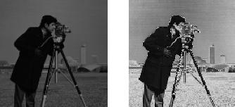
(a) Magnitude and argument

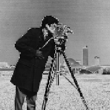
(b) Argument

(c) Magnitude and argument

Figure 1: (a) Ground-truth object, (b) ground-truth phase object and (c) window.

As background, we use the Shepp-Logan phantom in Figure 2 (a). Figure 2 (b) illustrates a diffraction pattern with background noise. Different levels of noise are simulated by adding different multiples of the phantom to the same diffraction patterns. To quantify the noise level, we use the ratio $\|Y-\tilde{Y}\|_{F}\big{/}\norm{Y}_{F},$ where $Y$ is as defined in (4) and $\tilde{Y}$ as in (7).

(a)

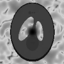
(b)

Figure 2: (a) Background and (b) exemplary diffraction pattern perturbed by background noise in logarithmic scale.

As quality metrics, relative reconstruction error and relative measurement error

$$\min_{\theta\in(0,2\pi]}\norm{x-e^{i\theta}\tilde{x}}_{2}\big{/}\norm{x}_{2},\quad\text{and}\quad\|Y-Y^{rec}\|_{F}\big{/}\norm{Y}_{F},$$

are used, where $x$ is the ground-truth, $\tilde{x}$ is the reconstructed object and $Y^{rec}_{\ell,r}=\left|\left(F\left[S_{-r}\tilde{x}\circ w\right]\right)_{\ell}\right|^{2}$, for all $\ell,r\in[d]$, are the simulated corresponding measurements.

In the following, we compare the object reconstruction obtained by the ‘vanilla’ WDD algorithm (Algorithm 1) with the reconstruction results of our algorithms, described in Algorithm 2 for general objects and in Algorithm 3 for phase objects.

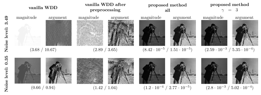
Figure 3: Comparison of the performance of the vanilla WDD algorithm (Algorithm 1) without and with preprocessing, and Algorithm 2 for different noise levels and different amounts of diagonals incorporated into the experiment (all or $\gamma=3$). Below the reconstruction results, find the respective (relative reconstruction error/measurement error).

In 2D, we interpret the parameter $\gamma$ in (A) for any $\gamma<\delta$ such that we consider all diagonals corresponding to tuples $j=(j_{1},j_{2})$ in

$$\mathcal{D}_{\gamma}\mathrel{\vbox{\hbox{\scriptsize.}\hbox{\scriptsize.}}}=\{(j_{1},j_{2})\in\mathbb{Z}^{2}:0\leq j_{1}<\gamma,\ -\gamma<j_{2}<\gamma,\ -\gamma<j_{1}+j_{2}<\gamma\}.$$

The case when all diagonals

$$\{(j_{1},j_{2})\in\mathbb{Z}^{2}:0\leq j_{1}<\delta,\ -\delta<j_{2}<\delta\}$$

are used is referred to as “all”.

All experiments were performed in Python on a MacBook Pro equipped with a 2GHz Intel Core i5 and 16 GB of memory.

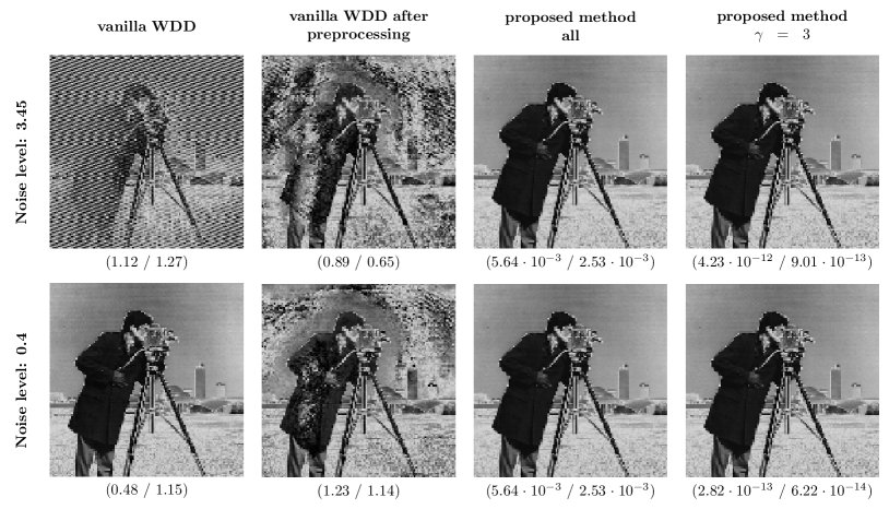
Figure 4: Comparison of the performance of the vanilla WDD algorithm (Algorithm 1) without and with preprocessing, and Algorithm 3 for different noise levels and different amounts of diagonals incorporated into the experiment (all or $\gamma=3$). Below the reconstruction results, find the respective (relative reconstruction error / measurement error).

$d$	$\delta$	run time (in seconds)			relative reconstruction error			relative measurement error
		WDD (all)	WDD ($\gamma=3$)	ADP	WDD (all)	WDD ($\gamma=3$)	ADP	WDD (all)	WDD ($\gamma=3$)	ADP
64	8	17	7	59	$1.6\cdot 10^{-4}$	$3.2\cdot 10^{-3}$	$0.29$	$5.1\cdot 10^{-5}$	$9.4\cdot 10^{-4}$	0.09
	16	62	10	64	$7.4\cdot 10^{-5}$	$2.1\cdot 10^{-3}$	$0.30$	$1.6\cdot 10^{-5}$	$4.9\cdot 10^{-4}$	0.15
96	8	47	41	812	$2.5\cdot 10^{-4}$	$1.7\cdot 10^{-3}$	$0.38$	$5.1\cdot 10^{-5}$	$5.5\cdot 10^{-4}$	0.08
	16	143	41	789	$5.5\cdot 10^{-5}$	$1.6\cdot 10^{-3}$	$0.31$	$1.2\cdot 10^{-5}$	$4.0\cdot 10^{-4}$	0.16

Table 2: Comparison of Algorithm 2 (WDD) with 10 iterations of the ADP algorithm chang2019advanced for ptychographic measurements with background noise causing a noise level of size approximately $3.5$.

First, we test Algorithm 2 on the object in Figure 1 (a). We compare the reconstructions obtained by our approach with the results of Algorithm 1. Apart from these two methods, we implemented the preprocessing approach by wang2017background . The results can be found in Figure 3.

As expected, vanilla WDD suffers from the noise. While preprocessing improves the reconstruction, it requires tuning the parameters for optimal performance depending on the noise level. In contrast, the method proposed by us filters the background noise and provides a good reconstruction independently of the noise level both when using all diagonals or only those in $\mathcal{D}_{3}$.

Now, we apply Algorithm 3 to reconstruct the phase object in Figure 1 (b) from its ptychographic measurements with background noise. Again, the reconstruction results are compared with Algorithm 1 with and without additional preprocessing wang2017background . As these methods are not expected to produce a phase object, the reconstructions are projected on $\mathbb{T}^{d\times d}$. Figure 4 shows that, again, our proposed algorithm filters the background noise well. Interestingly, the $\mathcal{D}_{3}$ version of Algorithm 3 shows better reconstruction errors while using less diagonals. This could be a result of a numerical error accumulation from a larger number of diagonals or a suboptimal outcome of the phase synchronization step.

Additionally, we compare the performance of our algorithms and the ADMM denoising algorithm for phase retrieval (ADP) proposed in chang2019advanced . In Table 2 and Table 3, we list the runtime, the relative reconstruction and measurement errors of the respective methods. For general objects, an additional comparison of Algorithm 2 both for all diagonals and for those in $\mathcal{D}_{3}$ is included. We observe that WDD reconstructs the ground-truth object up to a numerical error. ADP, on the other hand, requires more iterations and time to match the same precision.

$d$	$\delta$	run time (in seconds)		relative reconstruction error		relative measurement error
		WDD	ADP	WDD	ADP	WDD	ADP
64	8	5	61	$2.7\cdot 10^{-14}$	$0.95$	$1.0\cdot 10^{-14}$	0.29
	16	8	58	$5.7\cdot 10^{-14}$	$0.80$	$2.8\cdot 10^{-14}$	0.45
96	8	33	705	$1.9\cdot 10^{-13}$	$0.99$	$3.4\cdot 10^{-14}$	0.27
	16	37	778	$1.1\cdot 10^{-13}$	0.93	$3.8\cdot 10^{-14}$	0.44

Table 3: Comparison of Algorithm 3 (WDD with $\gamma=3$) with 10 iterations of the ADP algorithm chang2019advanced for ptychographic measurements of a phase object with background noise causing a noise level of size approximately $3.5$.

5 Proofs

5.1 Proof of Theorem 10

For $x\in\mathbb{T}^{d}$, by Proposition 9 we have

$$\left|\left(F^{-1}\left(F\left[x\circ S_{j}\overline{x}\right]\right)\right)_{\ell}\right|=\left|\left(x\circ S_{j}\overline{x}\right)_{\ell}\right|=1,$$ (19)

for all $\ell,j\in[d]$. We expand the inverse Fourier transform as

$$\left(F^{-1}\left(F\left[x\circ S_{j}\overline{x}\right]\right)\right)_{\ell}=\frac{1}{d}\sum_{k=0}^{d-1}e^{\frac{2\pi i\ell k}{d}}\left(F\left[x\circ S_{j}\overline{x}\right]\right)_{k}=\frac{1}{d}\left|f_{0}^{j}\right|e^{i\varphi_{j}}+\frac{1}{d}a_{\ell}^{j},$$ (20)

where the definitions (15) and (17) were used.

To obtain $\varphi_{j}$, we combine (19) and (20), and study the quadratic equation

$$d^{2}=\left||f_{0}^{j}|\cdot e^{i\varphi_{j}}+a_{\ell}^{j}\right|^{2},~{}~{}\ell\in[d].$$

Expanding the squares gives

$$\left||f_{0}^{j}|\cdot e^{i\varphi_{j}}+a_{\ell}^{j}\right|^{2} =|f_{0}^{j}|^{2}+2|f_{0}^{j}|\operatorname{Re}\left(a_{\ell}^{j}e^{-i\varphi_{j}}\right)+|a_{\ell}^{j}|^{2}$$

$$=|f_{0}^{j}|^{2}+2|f_{0}^{j}|\left(\operatorname{Re}(a_{\ell}^{j})\cos(\varphi_{j})+\operatorname{Im}(a_{\ell}^{j})\sin(\varphi_{j})\right)+|a_{\ell}^{j}|^{2},$$

and we rewrite the condition to be satisfied by $\varphi_{j}$ as

$$\operatorname{Re}(a_{\ell}^{j})\cos(\varphi_{j})+\operatorname{Im}(a_{\ell}^{j})\sin(\varphi_{j})=\frac{1}{2|f_{0}^{j}|}\left(d^{2}-|a_{\ell}^{j}|^{2}-|f_{0}^{j}|^{2}\right)$$

for all $\ell\in[d]$. That means, we need to solve (16) to recover $\varphi_{j}$.        $\blacksquare$

5.2 Proof of Theorem 11

Firstly, we show that, for all $m\in[d]$, the objects $x\sim\left(e^{\frac{2\pi i\ell m}{d}}\right)_{\ell\in[d]}$ with appropriately chosen background $b^{m}\in\mathbb{R}^{d}$ produce the same measurements.

Let $x^{m}\mathrel{\vbox{\hbox{\scriptsize.}\hbox{\scriptsize.}}}=\left(e^{\frac{2\pi i\ell m}{d}}\right)_{\ell\in[d]}$ for $m\in[d]$. Let $\tilde{Y}^{m}\in\mathbb{R}^{d\times d}$ be the respective measurements (7) for all $x^{m}$, $m\in[d]$, with some background noise $b^{m}\in\mathbb{R}^{d}$.

For all objects $x^{m}$, all diagonals are constant, more precisely

$$(x^{m}\circ S_{j}\overline{x^{m}})_{\ell}=e^{-\frac{2\pi ijm}{d}}$$ (21)

for all $\ell\in[d]$. Hence, for all $m,j\in[d]$, the respective Fourier coefficients $f^{j,m}_{k}$ are zero for all $k\in[d]\backslash\left\{0\right\}$. Consequently, for all $m,j\in[d],$ and all $k\in[d]\backslash\left\{0\right\}$, Proposition 8 provides $(F^{-1}\tilde{Y}^{0}F)_{j,k}=(F^{-1}\tilde{Y}^{m}F)_{j,k}$. For $k=0$, Proposition 8 tells that $(F^{-1}\tilde{Y}^{0}F)_{j,0}=(F^{-1}\tilde{Y}^{m}F)_{j,0}$ for all $j\in[d]$ if and only if

$$\left(f^{j,0}_{0}-f^{j,m}_{0}\right)(\overline{F[\overline{w}\circ S_{j}w]})_{0}=d(F^{-1}(b^{m}-b^{0}))_{j},$$

which is equivalent to

$$(F^{-1}(b^{m}-b^{0}))_{j}=\left(1-e^{-\frac{2\pi ijm}{d}}\right)(\overline{F[\overline{w}\circ S_{j}w]})_{0},$$

as from (21) we obtain $f^{j,m}_{0}=de^{-\frac{2\pi ijm}{d}}$.

Via this relation, we can define backgrounds $b^{m}$ which cause the same measurements for objects $x^{m}$. For example, we can set $(F^{-1}b^{0})_{j}=0$ for all $j\in[d]\backslash\left\{0\right\}$, and choose $(F^{-1}b^{0})_{0}\in\mathbb{R}$ suitably.

As $F^{-1}b^{0}$ is chosen conjugate symmetric, its Fourier transform $b^{0}$ is real-valued according to Corollary 2. Moreover, $F^{-1}b^{m}$ is conjugate symmetric since $(F^{-1}b^{m})_{0}=(F^{-1}b^{0})_{0}\in\mathbb{R}$ as $e^{-\frac{2\pi ijm}{d}}=1$ for $j=0$, and

$$\overline{(F^{-1}b^{m})_{-j}} =\overline{\left(1-e^{\frac{2\pi ijm}{d}}\right)}(F[\overline{w}\circ S_{-j}w])_{0}$$

$$=\left(1-e^{-\frac{2\pi ijm}{d}}\right)\overline{(F[\overline{w}\circ S_{j}w])}_{0}=(F^{-1}b^{m})_{j},$$

for all $j\in[d]\backslash\left\{0\right\}$, where we use the symmetry of

$$(F[\overline{w}\circ S_{-j}w])_{0}=\sum_{\ell=0}^{d-1}\overline{w}_{\ell}w_{\ell-j}=\sum_{\ell=0}^{d-1}\overline{w}_{\ell+j}w_{\ell}=\overline{(F[\overline{w}\circ S_{j}w])}_{0}.$$ (22)

Hence, also $b^{m}\in\mathbb{R}^{d}$ for all $m\in[d]$.

It remains to choose $(F^{-1}b^{0})_{0}\in\mathbb{R}$ large enough such that the backgrounds $b^{m}$ satisfy $b^{m}_{\ell}\geq-|F[S_{-r}x^{m}\circ w]_{\ell}|^{2}$, to ensure $\tilde{Y}^{m}_{\ell,r}\geq 0$ for all $m,\ell,r\in[d]$. The inverse Fourier transform gives

$$(F^{-1}b^{0})_{0}=(F^{-1}b^{m})_{0}\geq-|F[S_{-r}x^{m}\circ w]_{\ell}|^{2}-\sum_{j=1}^{d-1}e^{\frac{2\pi ij\ell}{d}}(F^{-1}b^{m})_{j}.$$

Taking the maximum on the right-hand side over $\ell,m\in[d]$ provides a suitable choice of $(F^{-1}b^{0})_{0}$.

We conclude that, with such background noise, objects $x^{m}$ produce the same measurements (7) and, thus, cannot be recovered uniquely.

Secondly, we show that for objects $x^{q},\ q=1,2,$ defined by entries

$$x_{\ell}^{q}=e^{-\frac{2\pi i\ell m}{d}}\cdot\begin{cases}1,\quad&\ell~{}\text{even},\\ -(-1)^{q}e^{(-1)^{q}\frac{1}{2}i\rho},&\ell~{}\text{odd},\end{cases},\quad\ell\in[d],$$ (23)

there exist backgrounds $b^{q},\ q=1,2,$ such that $(x^{1},b^{1})$ and $(x^{2},b^{2})$ result in the same measurements (7), i.e., there exist $b^{1},b^{2}\in\mathbb{R}^{d}$ with

$$\tilde{Y}^{1}_{\ell,r}\mathrel{\vbox{\hbox{\scriptsize.}\hbox{\scriptsize.}}}=\left|\left(F\left[S_{-r}x^{1}\circ w\right]\right)_{\ell}\right|^{2}+b^{1}_{\ell}=\left|\left(F\left[S_{-r}x^{2}\circ w\right]\right)_{\ell}\right|^{2}+b^{2}_{\ell}=\mathrel{\vbox{\hbox{\scriptsize.}\hbox{\scriptsize.}}}\tilde{Y}^{2}_{\ell,r},$$

for all $\ell,r\in[d]$.

Fix $m\in\mathbb{Z},\ \rho\in(-\pi,\pi)$, and consider objects $x^{q},\ q=1,2$, defined as in (23). The diagonals corresponding to the objects $x^{q},\ q=1,2,$ are given by

$$(x^{q}\circ S_{j}\overline{x^{q}})_{\ell}=\begin{cases}1,\quad&j~{}\text{even},\\ -(-1)^{q}e^{\frac{2\pi ijm}{d}-(-1)^{q}(-1)^{\ell}\frac{1}{2}i\rho},\quad&j~{}\text{odd},\end{cases}\quad\ell\in[d].$$

For $j$ even, the Fourier coefficients are

$$f^{j,q}_{k}=\begin{cases}d,\quad&k=0,\\ 0,\quad&k\in[d]\backslash\{0\},\end{cases}$$ (24)

and for $j$ odd, they are

$$f^{j,q}_{k} =-(-1)^{q}e^{\frac{2\pi ijm}{d}}\left(\sum_{\ell=0}^{\frac{d}{2}-1}e^{-\frac{2\pi ik\frac{\ell}{2}}{\frac{d}{2}}}e^{-(-1)^{q}\frac{1}{2}i\rho}+\sum_{\ell=0}^{\frac{d}{2}-1}e^{-\frac{2\pi ik\frac{\ell-1}{2}}{\frac{d}{2}}}e^{(-1)^{q}\frac{1}{2}i\rho}\right)$$

$$=\begin{cases}-(-1)^{q}e^{\frac{2\pi ijm}{d}}\cdot\frac{d}{2}\cos(\frac{\rho}{2}),\quad&k=0,\\ e^{\frac{2\pi ijm}{d}}\cdot\frac{d}{2}i\sin(\frac{\rho}{2}),\quad&k=\frac{d}{2},\\ 0,\quad&k\in[d]\backslash\{0,\frac{d}{2}\}.\end{cases}$$

Hence, for all $j\in[d]$ and all $k\in[d]\backslash\{0\}$, we know $f^{j,1}_{k}=f^{j,2}_{k}$, so that Proposition 8 guarantees $(F^{-1}\tilde{Y}^{1}F)_{j,k}=(F^{-1}\tilde{Y}^{2}F)_{j,k}$. For $k=0$, again, it holds $(F^{-1}\tilde{Y}^{1}F)_{j,0}=(F^{-1}\tilde{Y}^{2}F)_{j,0}$ for all $j\in[d]$ if and only if

$$\left(f^{j,1}_{0}-f^{j,2}_{0}\right)(\overline{F[\overline{w}\circ S_{j}w]})_{0}=d(F^{-1}(b^{2}-b^{1}))_{j}.$$

Analogously to the above, we can conclude that there exists background noise with which objects $x^{1}$ and $x^{2}$ produce the same measurements (7), i.e., unique recovery of objects $x^{1}$ or $x^{2}$ is also not possible.        $\blacksquare$

5.3 Analysis of linear systems (16)

In this section, the foundation of the proof of Theorem 12 is established by studying the linear systems (16). For any $j\in[d]$, the three possible cases $\rank(A^{j})=0,\ \rank(A^{j})=1,$ and $\rank(A^{j})=2$ are investigated.

In the following, we write $F^{-1}f^{j}$ instead of $x\circ S_{j}\overline{x}$ as there is not necessarily a unique $x$ corresponding to $F^{-1}f^{j}$.

We start with the case $\rank(A^{j})=0$.

Lemma 13.

Let $j\in[d]$. The following claims are equivalent:

1. The matrix $A^{j}$ has $\rank(A^{j})=0$.

2. $(F^{-1}f^{j})_{k}=e^{i\varphi_{j}}$ for all $k\in[d]$, where $\varphi_{j}$ is as in (15).

3. The zeroth Fourier coefficient admits $|f^{j}_{0}|=d$.

Furthermore, if $\rank(A^{j})=0$ and $j$ is coprime with $d$, the ground-truth object is $x\sim\left(e^{\frac{2\pi ikm}{d}}\right)_{k\in[d]}$, for some $m\in[d]$.

Proof: [Proof.] $(i)\Rightarrow(ii),(iii):$ Let $\rank(A^{j})=0$. Definition (17) gives $a_{\ell}^{j}=0$ for all $\ell\in[d]$. We then obtain

$$d(F^{-1}f^{j})_{\ell}=\sum_{k=0}^{d-1}e^{\frac{2\pi ik\cdot\ell}{d}}f^{j}_{k}=a_{\ell}^{j}+f_{0}^{j}=f_{0}^{j}=|f_{0}^{j}|e^{i\varphi_{j}},$$

for all $\ell\in[d]$, i.e., $F^{-1}f^{j}$ has constant value $f_{0}^{j}/d$. By Proposition 9, $F^{-1}f^{j}\in\mathbb{T}^{d}$ and, thus, $F^{-1}f^{j}=e^{i\varphi_{j}}$ and $|f_{0}^{j}|=d$.

$(ii)\Rightarrow(iii):$ If $(F^{-1}f^{j})_{\ell}=e^{i\varphi_{j}}\in\mathbb{T}$ for all $\ell\in[d]$, we get

$$f^{j}_{k}=(F(F^{-1}f^{j}))_{k}=\sum_{\ell=0}^{d-1}e^{\frac{-2\pi ik\cdot\ell}{d}}e^{i\varphi_{j}}=\begin{cases}de^{i\varphi_{j}},\quad&k=0,\\ 0,\quad&k\in[d]\backslash\{0\},\end{cases}$$

and, hence, $|f^{j}_{0}|=d|e^{i\varphi_{j}}|=d$.

$(iii)\Rightarrow(i):$ If $|f^{j}_{0}|=d$, by Proposition 9, the definition in (17), and Plancherel’s identity (2) we have

$$\norm{a^{j}}_{2}^{2}=\tfrac{1}{d}\norm{Fa^{j}}_{2}^{2}=d\norm{(0,f_{1}^{j},\ldots,f_{d-1}^{j})}_{2}^{2}=d\norm{f^{j}}_{2}^{2}-d|f^{j}_{0}|^{2}=d^{3}-d^{3}=0.$$

That means, $a^{j}_{k}=0$ for all $k\in[d]$, and $\rank(A^{j})=0$.

In addition to $\rank(A^{j})=0$, let us assume that $j$ is coprime with $d$. Consider any $x\in\mathbb{T}^{d}$ with $x\circ S_{j}\overline{x}=F^{-1}f^{j}$. From the equivalence of $(i)$ and $(ii)$ proven above, we find that $x_{k}\overline{x}_{k+j}=(F^{-1}f^{j})_{k}=e^{i\varphi_{j}}$ for all $k\in[d]$, i.e.,

$$\arg(x_{k})-\arg(x_{k+j})=\varphi_{j}+2\pi m$$ (25)

for some $m\in\mathbb{Z}$. With this, we obtain

$$\arg(x_{\ell j})\in\arg(x_{0})-\ell\varphi_{j}+2\pi\mathbb{Z}$$

for any $\ell\in\mathbb{Z}$. Since $j$ and $d$ are coprime, $\ell=d$ is the smallest integer satisfying $\ell j=0\operatorname{mod}d$. We conclude that

$$\arg(x_{0})=\arg(x_{dj})\in\arg(x_{0})-d\varphi_{j}+2\pi\mathbb{Z},$$

hence, $\varphi_{j}\in\frac{2\pi}{d}\mathbb{Z}$. Combining this with (25), we find that the corresponding objects are of the type $x\sim\left(e^{\frac{2\pi ikm}{d}}\right)_{k\in[d]}$, for some $m\in\mathbb{Z}$.

Next, we study the system (16) in case $\rank(A^{j})=1$.

Lemma 14.

Let $j\in[d]$ and $\rank(A^{j})=1$. There exist two solutions $\varphi^{j}_{1}\neq\varphi^{j}_{2}$ to (16) given by

$$\varphi^{j}_{q}\mathrel{\vbox{\hbox{\scriptsize.}\hbox{\scriptsize.}}}=\arg(a_{0}^{j})+(-1)^{q}\arccos\left(\frac{d^{2}-|a_{0}^{j}|^{2}-|f_{0}^{j}|^{2}}{2|a_{0}^{j}||f_{0}^{j}|}\right),\quad q=1,2.$$

Furthermore, there exists a disjoint partition $\mathcal{S}_{j},\mathcal{S}_{j}^{c}$ of $[d]$ such that $0\in\mathcal{S}_{j}$, $\mathcal{S}_{j}^{c}\neq\varnothing$, and we can write the corresponding diagonals $F^{-1}f^{j,q}$ as

$$(F^{-1}f^{j,q})_{k}=\begin{cases}e^{i\psi^{j}_{q}},&k\in\mathcal{S}_{j},\\ e^{i(\psi^{j}_{q}+(-1)^{q}\rho^{j})},&k\in\mathcal{S}_{j}^{c},\end{cases}\quad q=1,2,$$

with $\rho^{j}\in(-\pi,\pi)\backslash\{0\}$, $\psi_{1}^{j}\neq\psi_{2}^{j},$ and

$$\psi_{2}^{j}\in\psi_{1}^{j}-\rho^{j}+\pi+2\pi\mathbb{Z}.$$ (26)

Proof: [Proof.]

Lemma 14 can be interpreted geometrically as a problem of intersecting circles. For a visualization of the proof idea, see Figure 5.

Figure 5: Geometric visualization of Lemma 14. By Proposition 9, $|f_{0}^{q}|$ is known. This guarantees that the possible Fourier coefficients $f^{q}_{0}$ lie on the blue circle. By definition, $f_{0}^{q}+a_{\ell}=d(F^{-1}f^{q})_{\ell}$ and $|(F^{-1}f^{q})_{\ell}|=1$. Hence, $f_{0}^{q}+a_{\ell}$ has to lie on the green circle. Consequently, the possible solutions $f^{q}_{0}$ lie on the orange circle, or, more precisely, on its intersections with the blue circle. It can be shown that neither the blue and the green circle coincide nor the orange circle is tangent to the blue circle, so that there are precisely two intersection points, corresponding to two solutions. The lightgray dotted lines are parallels in the direction of $a_{0}$ containing the solutions $f^{q}_{0}$. Their two intersection with the green circle show that there are two distinct values the entries of the diagonal can take.

In the following, let $j\in[d]$ be fixed. Throughout the proof, we drop the index $j$ to simplify the notation.

Since $\rank(A)=1$, all equations in (16) are the same up to a multiplicative constant $c_{k}\in\mathbb{R},$ i.e.,

$$a_{k}=c_{k}\cdot a_{0},$$ (27)

for all $k\in[d]\backslash\{0\}.$ If, for some $k\in[d]\backslash\{0\}$, we have $|a_{k}|=0$, the corresponding equation

$$\operatorname{Re}(a_{k})\cos(\varphi)+\operatorname{Im}(a_{k})\sin(\varphi)=\frac{1}{2|f_{0}|}\left(d^{2}-|a_{k}|^{2}-|f_{0}|^{2}\right)$$

in (16) reduces to $d=|f_{0}|$. By Lemma 13, this is equivalent to $\rank(A)=0$, which contradicts $\rank(A)=1$. Hence, $|a_{k}|>0$ and $c_{k}\neq 0$ for all $k\in[d]\backslash\{0\}$.

We can rewrite the equations of (16) as

$$d^{2}=|a_{k}|^{2}+|f_{0}|^{2}+2|f_{0}|\operatorname{Re}\left(a_{k}e^{-i\varphi}\right).$$

Since (16) is only considered for $|f_{0}|>0$, it is further transformed into

$$\cos(\arg(a_{k})-\varphi)=\frac{d^{2}-|a_{k}|^{2}-|f_{0}|^{2}}{2|a_{k}||f_{0}|},$$

which may have two solutions

$$\varphi_{q}=\arg(a_{k})+(-1)^{q}\arccos\left(\frac{d^{2}-|a_{k}|^{2}-|f_{0}|^{2}}{2|a_{k}||f_{0}|}\right),\quad q=1,2.$$

As the system (16) has at least one solution corresponding to the ground-truth object $x$, the right-hand side is the same for all $k\in[d]$. Setting $k=0$ gives the desired formula for $\varphi_{q}$, $q=1,2$.

Note that $\varphi_{1}=\varphi_{2}$ if and only if, for all $k\in[d]$,

$$\frac{d^{2}-|a_{k}|^{2}-|f_{0}|^{2}}{2|a_{k}||f_{0}|}=\delta,$$

for $\delta\in\left\{-1,1\right\}$. Bringing the denominator to the other side and summing the equations for all $k$ yields

$$d^{3}-\sum_{k=0}^{d-1}|a_{k}|^{2}-d|f_{0}|^{2}=2\delta|f_{0}|\sum_{k=0}^{d-1}|a_{k}|.$$ (28)

Plancherel’s identity (2) combined with (17) and Proposition 9 gives

$$\norm{a}_{2}^{2}=\tfrac{1}{d}\norm{Fa}_{2}^{2}=d\norm{(0,f_{1},\ldots,f_{d-1})}_{2}^{2}=d\norm{f}_{2}^{2}-d|f_{0}|^{2}=d^{3}-d|f_{0}|^{2}.$$

Substituting this into (28) results in

$$2|f_{0}|\sum_{k=0}^{d-1}|a_{k}|=0.$$

Recall that the case $|f_{0}|=0$ is excluded as it does not require solving the linear system (16). Moreover, we showed above that all $a_{k}\neq 0$. Hence, in the case $\rank(A)=1$, there always exist two values $\varphi_{1}\neq\varphi_{2}$ solving (16). In the following, the corresponding two vectors of Fourier coefficients are denoted by $f^{1}$ and $f^{2}$, respectively.

These solutions can be described in more detail. Let us set $\psi_{q}$ so that

$$\left(F^{-1}f^{q}\right)_{0}=e^{i\psi_{q}}.$$

By the definitions (9), (17), and (27), we obtain

$$f_{0}^{q}+c_{k}a_{0}=f_{0}^{q}+a_{k}=\sum_{\ell=0}^{d-1}e^{\frac{2\pi ik\ell}{d}}f^{q}_{\ell}=d(F^{-1}f^{q})_{k}.$$

By Proposition 9, the diagonals satisfy $F^{-1}f^{q}\in\mathbb{T}^{d}$. Thus, we have that $\tfrac{1}{d}(f_{0}^{q}+c_{k}a_{0})\in\mathbb{T}$.

The system (16) has at least one solution corresponding to the ground-truth object $x$. Consequently, the right-hand side of (16) belongs to

$$\operatorname{im}(A)\mathrel{\vbox{\hbox{\scriptsize.}\hbox{\scriptsize.}}}=\{v\in\mathbb{R}^{d}:Au=v\ \text{for some}\ u\in\mathbb{R}^{2}\}.$$

For every $v\in\operatorname{im}(A)$ we have

$$v_{k}=\operatorname{Re}(a_{k})u_{1}+\operatorname{Im}(a_{k})u_{2}=c_{k}\operatorname{Re}(a_{0})u_{1}+c_{k}\operatorname{Im}(a_{0})u_{2}=c_{k}v_{0},$$

and, thus, the right-hand side of (16) also admits

$$1-\frac{1}{d^{2}}\left(|a_{k}|^{2}+|f_{0}|^{2}\right)=c_{k}\left[1-\frac{1}{d^{2}}\left(|a_{0}|^{2}+|f_{0}|^{2}\right)\right].$$ (29)

Inserting (27) into (29), we obtain

$$d^{2}-c_{k}^{2}|a_{0}|^{2}-|f_{0}|^{2}=c_{k}\cdot\left(d^{2}-|a_{0}|^{2}-|f_{0}|^{2}\right).$$

This quadratic equation with respect to $c_{k}$ has two roots, $1$ and $c\mathrel{\vbox{\hbox{\scriptsize.}\hbox{\scriptsize.}}}=(|f_{0}|^{2}-d^{2})/|a_{0}|^{2}<0$, noticeably, independent of $k$. Let us define $\mathcal{S}$ and $\mathcal{S}^{c}$ as

$$\mathcal{S}\mathrel{\vbox{\hbox{\scriptsize.}\hbox{\scriptsize.}}}=\{k\in[d]:c_{k}=1\}\quad\text{and}\quad\mathcal{S}^{c}\mathrel{\vbox{\hbox{\scriptsize.}\hbox{\scriptsize.}}}=\{k\in[d]:c_{k}=c\}.$$

By construction, $0\in\mathcal{S}$, $\mathcal{S}\cap\mathcal{S}^{c}=\varnothing,$ and $\mathcal{S}\cup\mathcal{S}^{c}=[d]$. If $\mathcal{S}^{c}$ is empty, the entries of $(F^{-1}f^{q})$ are all equal to $\tfrac{1}{d}(f_{0}^{q}+a_{0})$, which, by Lemma 13, contradicts the $\rank(A)=1$ assumption. Thus, we conclude that $\mathcal{S}^{c}\neq\varnothing$.

Then, for both, $q=1$ and $q=2$, the values of $F^{-1}f^{q}$ are given by

$$(F^{-1}f^{q})_{k}=\tfrac{1}{d}(f_{0}^{q}+a_{0})=e^{i\psi_{q}},\quad k\in\mathcal{S},$$

and

$$(F^{-1}f^{q})_{k}=\tfrac{1}{d}(f_{0}^{q}+ca_{0})=\mathrel{\vbox{\hbox{\scriptsize.}\hbox{\scriptsize.}}}e^{i(\psi_{q}+\rho_{q})},\quad k\in\mathcal{S}^{c},$$

for some $\rho_{q}\in(-\pi,\pi]\backslash\{0\}$.

The next step is to show that $\rho_{2}=-\rho_{1}$. We have

$$e^{i(\psi_{q}+\rho_{q})}=\tfrac{1}{d}(f_{0}^{q}+ca_{0}+a_{0}-a_{0})=e^{i\psi_{q}}+(c-1)\cdot\frac{1}{d}a_{0},\quad q=1,2.$$

Combining the two relations for $q=1$ and $q=2$ yields

$$e^{i\psi_{1}}\left(1-e^{i\rho_{1}}\right)=e^{i\psi_{2}}\left(1-e^{i\rho_{2}}\right).$$ (30)

Since $|e^{i\psi_{1}}|=|e^{i\psi_{2}}|=1$, we get

$$|1-e^{i\rho_{1}}|^{2}=|1-e^{i\rho_{2}}|^{2},$$

or, equivalently,

$$\cos\rho_{1}=\cos\rho_{2}.$$

As we choose $\rho_{1},\rho_{2}\in(-\pi,\pi]\backslash\left\{0\right\}$, either $\rho_{2}=\rho_{1}$ or $\rho_{2}=-\rho_{1}$ holds. If $\rho_{2}=\rho_{1}$, then (30) yields $\psi_{1}=\psi_{2}$ and $f^{1}_{0}=f^{2}_{0}$, which in turn, implies $\varphi_{1}=\varphi_{2}$ and contradicts $\varphi_{1}\neq\varphi_{2}$. We conclude that $\rho_{2}=-\rho_{1}$.

In particular, for $\rho_{1}=\pi$, the only $\rho_{2}\in(-\pi,\pi]\backslash\{0\}$ satisfying $\cos(\rho_{2})=\cos(\rho_{1})=-1$ is $\rho_{2}=\pi=\rho_{1}$, contradicting $\rho_{2}\neq\rho_{1}$. Therefore, we have $\rho_{1}\in(-\pi,\pi)\backslash\{0\}$.

Finally, via (30), we obtain

$$e^{i\psi_{1}}=e^{i\psi_{2}}\cdot\frac{e^{-i\rho_{1}}-1}{e^{i\rho_{1}}-1}=e^{i\psi_{2}}\cdot(-e^{-i\rho_{1}})=e^{i\psi_{2}}\cdot e^{-i\rho_{1}}\cdot e^{i\pi},$$

so that

$$\psi_{1}=\psi_{2}-\rho_{1}+\pi+2\pi m$$

for some $m\in\mathbb{Z}$. Setting $\rho=\rho_{2}=-\rho_{1}$, we obtain the statement of the lemma.

The remaining case to consider is $\rank(A^{j})=2$. In this case, system (16) is uniquely solvable. Hence, the lost zero frequency $f_{0}^{j}=\left(F\left[x\circ S_{j}\overline{x}\right]\right)_{0}$ can be recovered uniquely. Then, $x$ can be recovered uniquely if, additionally, $j$ is coprime with the object’s dimension $d$.

Lemma 15.

Let $j\in[d]$.

• If $\rank(A^{j})=2$, $\varphi_{j}$ is uniquely recoverable from (16), i.e., $F^{-1}f^{j}$ is uniquely recoverable from measurements (7).

• If $j$ is coprime with $d$, $x$ can be uniquely recovered from the diagonal $F^{-1}f^{j}=x\circ S_{j}\overline{x}$.

Proof: [Proof.] If $\rank(A^{j})=2$, system (16) has one solution, i.e., we can recover $\varphi_{j}$, and, hence, $\left(F\left[x\circ S_{j}\overline{x}\right]\right)_{0}$ uniquely. From $F\left[x\circ S_{j}\overline{x}\right]$, we obtain back $x\circ S_{j}\overline{x}$.

If $j$ and $d$ are coprime, $j$ is a generator of the additive group of integers modulo $d$, denoted by $\mathbb{Z}_{d}$. That means, for every $k\in[d]$, there exists $r\in\mathbb{Z}$ with $rj\operatorname{mod}d=k$. Hence, for any $k\in[d]$, there exists $r\in\mathbb{Z}$ with

$$x_{0}\overline{x}_{k}=\prod_{t=1}^{r}x_{(t-1)j}\overline{x}_{tj}\ \bigg{/}\ \prod_{t=1}^{r-1}|x_{tj}|^{2}.$$

Consequently, for all $k\in[d]$, the product $x_{0}\overline{x}_{k}$ can be built from the entries of $x\circ S_{j}\overline{x}$ together with the magnitudes of $x$, which are a priori known for a phase object. The phase of $x_{0}\in\mathbb{T}$ can be chosen arbitrarily as the solution to a phase retrieval problem is unique only up to a global phase. Based on this choice, the phases of $x_{k}\in\mathbb{T}$ for all $k>0$ are found using the relations $x_{0}\overline{x}_{k}$.

Remark 16.

If $j$ is not coprime with $d$, $j$ does not generate $\mathbb{Z}_{d}$. That means, $\mathcal{C}_{0}\mathrel{\vbox{\hbox{\scriptsize.}\hbox{\scriptsize.}}}=\left\{j\ell\operatorname{mod}d,\ell\in[d]\right\}\neq\mathbb{Z}_{d}$, and there exists at least one $n\in\mathbb{Z}_{d}$ such that $\mathcal{C}\mathrel{\vbox{\hbox{\scriptsize.}\hbox{\scriptsize.}}}=\{(j\ell+n)\operatorname{mod}d,\ell\in[d]\}$ satisfies $\mathcal{C}_{0}\cap\mathcal{C}=\varnothing$. Hence, for every object $x\in\mathbb{C}^{d}$ we can construct $\tilde{x}$ as

$$\tilde{x}_{k}=\begin{cases}\alpha x_{k},&k\in\mathcal{C},\\ x_{k},&k\notin\mathcal{C},\end{cases}$$

with $\alpha\in\mathbb{T}~{}\backslash\left\{1\right\}$, such that $\tilde{x}\not\sim x$ but $x\circ S_{j}\overline{x}=\tilde{x}\circ S_{j}\overline{\tilde{x}}$.

5.4 Proof of Theorem 12

In this section, we prove Theorem 12. Using the results of Section 5.3, we investigate in closer detail under which conditions system (16) is uniquely solvable. We will find that it is sufficient to use the information given by $j=1$ and $j=2$ to fully characterize the uniqueness of reconstruction for measurements with background noise. The proof is split into the analysis of the disjoint cases listed in Table 1.

The case $j=0$ is of no relevance as

$$\left(F\left[x\circ S_{0}\overline{x}\right]\right)_{0}=\sum_{k=0}^{d-1}e^{-\frac{2\pi ik\cdot 0}{d}}\cdot|x_{k}|^{2}=d$$

is known for a phase object, and does not provide further information on the phases of the object.

We start with investigating $j=1$. As $1$ is coprime with any $d\in\mathbb{N}$, Lemma 15 guarantees unique recovery in case $\rank(A^{1})=2$.

Let $\rank(A^{1})=0$. With $1$ being coprime with any $d\in\mathbb{N}$, Lemma 13 provides that the only object satisfying this condition is the negative example $(i)$ in Theorem 11. In Section 5.2 we showed that for this class of objects unique recovery is not possible.

If $\rank(A^{1})=1$, Lemma 14 tells that considering only the diagonal corresponding to shift $j=1$ is not sufficient. Thus, we need to include information for further diagonals.

We continue with $j=2$ and use that the first and the second off-diagonal are related via

$$(F^{-1}f^{2})_{k} =(x\circ S_{2}\overline{x})_{k}=x_{k}\cdot 1\cdot\overline{x_{k+2}}=x_{k}~{}|x_{k+1}|^{2}~{}\overline{x_{k+2}}$$ (31)

$$=(x\circ S_{1}\overline{x})_{k}~{}(x\circ S_{1}\overline{x})_{k+1}=(F^{-1}f^{1})_{k}~{}(F^{-1}f^{1})_{k+1}.$$

Again, the three possible cases $\rank(A^{2})=0$, $\rank(A^{2})=1$, and $\rank(A^{2})=2$ are considered.

Firstly, we find that $\rank(A^{2})=1$ is not feasible if $\rank(A^{1})=1$.

Lemma 17.

The case $\rank(A^{1})=1$ and $\rank(A^{2})=1$ is not possible.

Proof: [Proof.] We show the statement by contradiction. Assume that $\rank(A^{1})=\rank(A^{2})=1$. As $\rank(A^{1})=1$, Lemma 14 for $j=1$ states that there are the two distinct solutions

$$(F^{-1}f^{1,q})_{k}=\begin{cases}e^{i\psi_{q}},&k\in\mathcal{S},\\ e^{i(\psi_{q}+(-1)^{q}\rho)},&k\in\mathcal{S}^{c},\end{cases}\quad q=1,2,$$

with $\mathcal{S},\mathcal{S}^{c}$ as described in the proof of Lemma 14.

Here, we drop the index $j$ for $\psi^{j}_{q}$ and $\rho^{j}$ to shorten the notation as we only require these values for $j=1$. However, we keep the index in $f^{j,q}$ to distinguish $f^{1,q}$ and $f^{2,q}$.

By (31), there are three possible values which the entries of the second diagonal can take,

$$(F^{-1}f^{2,q})_{k} =(F^{-1}f^{1,q})_{k}(F^{-1}f^{1,q})_{k+1}$$

$$=\begin{cases}e^{i2\psi_{q}},&k\in\mathcal{S},\ k+1\in\mathcal{S},\\ e^{i(2\psi_{q}+(-1)^{q}\rho)},&k\in\mathcal{S},\ k+1\in\mathcal{S}^{c}\\ &\text{or}~{}k\in\mathcal{S}^{c},\ k+1\in\mathcal{S},\\ e^{i\left(2\psi_{q}+(-1)^{q}2\rho\right)},&k\in\mathcal{S}^{c},\ k+1\in\mathcal{S}^{c},\end{cases}$$ (32)

for both $q=1$ and $q=2$. However, since $\rank(A^{2})=1$, by Lemma 14, the second diagonal can only accept two different values. The index sets $\mathcal{S},\mathcal{S}^{c}\neq\varnothing$, hence there is at least one $k\in[d]$ with

$$\left(F^{-1}f^{1,q}\right)_{k}=e^{i\psi_{q}}\quad\text{and}\quad\left(F^{-1}f^{1,q}\right)_{k+1}=e^{i(\psi_{q}+(-1)^{q}\rho)}.$$

Thus, we can conclude for the second diagonal that

$$(F^{-1}f^{2,q})_{k}=e^{i\psi_{q}}\cdot e^{i(\psi_{q}+(-1)^{q}\rho)}=e^{i(2\psi_{q}+(-1)^{q}\rho)}$$

for at least one $k\in[d]$. Consequently,

$$(F^{-1}f^{2,q})_{k}\in\left\{e^{i(2\psi_{q}+(-1)^{q}\ell\rho)},e^{i\left(2\psi_{q}+(-1)^{q}(\ell+1)\rho\right)}\right\},\quad q=1,2,$$

where in both cases $\ell$ is either zero or one, depending on the set $\mathcal{S}$.

From Lemma 14 for $j=1$, we obtain

$$\psi_{1}=\psi_{2}+\rho+\pi+2\pi m_{1},$$ (33)

and, for $j=2$,

$$2\psi_{1}-\ell\rho=2\psi_{2}+\ell\rho+\rho+\pi+2\pi m_{2}$$ (34)

for some $m_{1},m_{2}\in\mathbb{Z}$.

Bringing $\psi_{1}-\psi_{2}$ to the left–hand side and the rest to the right-hand side in both (33) and (34) yields

$$\rho+\pi+2\pi m_{1}=\frac{1}{2}\left((2\ell+1)\rho+\pi+2\pi m_{2}\right),$$

so that

$$(2\ell-1)\rho=\pi+2\pi(2m_{1}-m_{2}).$$

For both, $\ell=0$ and $\ell=1$, we find that $\rho\in\left\{-\pi,\pi\right\}$, which is not attainable according to Lemma 14. Hence, $\rank(A^{1})=\rank(A^{2})=1$ is not feasible.

Next, we investigate the case $\rank(A^{1})=1$ and $\rank(A^{2})=0$ and find the second negative example $(ii)$ in Theorem 11. From Section 5.2 it is known that such objects cannot be recovered uniquely.

Lemma 18.

Let $x^{q}\in\mathbb{C}^{d}$ be defined by entries

$$x_{k}^{q}\mathrel{\vbox{\hbox{\scriptsize.}\hbox{\scriptsize.}}}=e^{-\frac{2\pi ikm}{d}}\cdot\begin{cases}1,\quad&k~{}\text{even},\\ -(-1)^{q}e^{(-1)^{q}\frac{1}{2}i\rho},&k~{}\text{odd},\end{cases}$$

for all $k\in[d]$. If $\rank(A^{1})=1$ and $\rank(A^{2})=0$, then $d$ is even and $x\sim x^{q}$ with $q=1$ or $q=2$ for some $m\in\mathbb{Z}$ and $\rho\in(-\pi,\pi)\backslash\{0\}$.

Proof: [Proof.]

According to Lemma 13, $\rank(A^{2})=0$ is equivalent to $F^{-1}f^{2}$ constant.

We assume $\rank(A^{1})=1$. As in Lemma 14, set $(F^{-1}f^{1,q})_{0}\mathrel{\vbox{\hbox{\scriptsize.}\hbox{\scriptsize.}}}=e^{i\psi_{q}}$ for some $\psi_{q}\in[0,2\pi),\ q=1,2$, and the other value that appears for at least one $(F^{-1}f^{1,q})_{k}$ we set as $e^{i(\psi_{q}+(-1)^{q}\rho)}$ for $\rho\in(-\pi,\pi)\backslash\{0\}$, for both $q=1,2$.

The first and the second off-diagonal are related via (31). Hence, based on the knowledge of the first diagonals $F^{-1}f^{1,q}$ and the fact that $F^{-1}f^{2}$ is constant, the second diagonal must be $(F^{-1}f^{2})_{k}=e^{i(2\psi_{q}+(-1)^{q}\rho)}$ for all $k\in[d]$, for either $q=1$ or $q=2$. For this to hold true, the entries of $F^{-1}f^{1,q}$ have to satisfy

$$\left(F^{-1}f^{1,q}\right)_{k}=\begin{cases}e^{i\psi_{q}},\quad&k~{}\text{even},\\ e^{i(\psi_{q}+(-1)^{q}\rho)},&k~{}\text{odd}.\end{cases}$$ (35)

If $d$ is odd, this means $x_{d-1}\overline{x}_{0}=e^{i\psi_{q}}$, so

$$x_{d-1}\overline{x}_{1}=x_{d-1}\overline{x}_{0}x_{0}\overline{x}_{1}=e^{i2\psi_{q}}.$$

This requires $\rho\in 2\pi\mathbb{Z}$. Then, the first diagonal is $\left(F^{-1}f^{1,q}\right)_{k}=e^{i\psi_{q}}$ for all $k\in[d]$, contradicting $\rank(A^{1})=1$. Hence, $\rank(A^{1})=1$ and $\rank(A^{2})=0$ can only appear if the object dimension $d$ is even.

Let $d$ be even. By

$$\prod_{k=0}^{d-1}x_{k}\overline{x}_{k+1}=\prod_{k=0}^{d-1}|x_{k}|^{2}=1,$$

we obtain

$$\left(e^{i\psi_{1}}\right)^{\frac{d}{2}}\left(e^{i(\psi_{1}-\rho)}\right)^{\frac{d}{2}}=1,$$

i.e.,

$$d\psi_{1}-\frac{d}{2}\rho=2\pi m$$ (36)

for some $m\in\mathbb{Z}$. Equation (26) in Lemma 14 further provides that the respective $\psi_{2}$ corresponding to $f^{1,2}$ satisfies $\psi_{2}=\psi_{1}-\rho-\pi+2\pi\tilde{m}$ for some $\tilde{m}\in\mathbb{Z}$.

The first diagonal is sufficient to reconstruct $x$ as explained in Lemma 15. From (35), we derive the two possible solutions

$$x_{k}^{q}=e^{-ik(\psi_{q}+(-1)^{q}\rho)}\cdot\begin{cases}e^{(-1)^{q}i\frac{k}{2}\rho},\quad&k~{}\text{even},\\ e^{(-1)^{q}i\frac{k+1}{2}\rho},&k~{}\text{odd},\end{cases}\quad q=1,2.$$

Together with (26) and (36), we obtain that $x$ can be equal to $x^{q}$ for $q=1$ or $q=2$ with

$$x_{k}^{q}=e^{-\frac{2\pi ikm}{d}}\cdot\begin{cases}1,\quad&k~{}\text{even},\\ -(-1)^{q}e^{(-1)^{q}\frac{1}{2}i\rho},&k~{}\text{odd},\end{cases}\quad q=1,2,$$

for all $k\in[d]$, for some $m\in\mathbb{Z}$ and $\rho\in(-\pi,\pi)\backslash\{0\}$.

Remark 19.

In Theorem 11 $(ii)$, we do not exclude $\rho=0$. Note that for $\rho=0$, the objects of type $(ii)$ equal the objects of type $(i)$. In Lemma 18, however, $\rho=0$ is excluded as it is not attainable in case $\rank(A^{1})=1$.

The remaining case to investigate is $\rank(A^{2})=2$. If $\rank(A^{2})=2$ and $d$ is odd, $d$ is coprime with $2$ and the ground-truth solution $x$ can be uniquely recovered as shown in Lemma 15 for $j=2$. It is left to study the case when $d$ is even.

Lemma 20.

If $\rank(A^{1})=1$, $\rank(A^{2})=2,$ and $d$ is even, the ground-truth solution $x$ can be uniquely recovered.

Proof: [Proof.]

If $\rank(A^{2})=2$, the system (16) for $j=2$ has one solution. That means, we can recover $f^{2}_{0}$ uniquely and compute the second diagonal $F^{-1}f^{2}$.

Since $d$ is even, $d$ and $j=2$ are not coprime and there are multiple $x$ corresponding to the second diagonal $F^{-1}f^{2}$, see Remark 16. However, we can make use of $f^{2}$ to select the ground-truth solution out of the two possible solutions $f^{1,1}\neq f^{1,2}$ obtained in Lemma 14 for the shift $j=1$. We show that this is possible by contradiction.

Assume that $f^{1,1}$ and $f^{1,2}$ yield, via (31), the same diagonal $F^{-1}f^{2}$. The entries of $F^{-1}f^{2}$ can be deduced from $f^{1,1}$ and $f^{1,2}$ and can take the three possible values as in (5.4) for both $q=1$ and $q=2$.

It is not possible that $F^{-1}f^{2}$ is constant. Otherwise, $\rank(A^{2})=0$ according to Lemma 13. Thus, for at least one $k\in[d]$,

$$(F^{-1}f^{2})_{k}\in\left\{e^{i2\psi_{q}},e^{i(2\psi_{q}+(-1)^{q}2\rho)}\right\}$$

for both $q=1,2$, and, as we assumed that $F^{-1}f^{2}$ is obtained from both $f^{1,1}$ and $f^{1,2}$, either

$$(i)\quad e^{i2\psi_{1}}=e^{i2\psi_{2}}\quad\text{or}\quad(ii)\quad e^{i(2\psi_{1}-2\rho)}=e^{i(2\psi_{2}+2\rho)}$$

must be satisfied. Suppose $(i)$ holds true. Then

$$2\psi_{1}=2\psi_{2}+2\pi m$$

for some $m\in\mathbb{Z}$, i.e.,

$$\psi_{1}=\psi_{2}+\pi m.$$

For $m$ even this means $\psi_{1}=\psi_{2}$ since $\psi_{1},\psi_{2}\in(0,2\pi]$, which is impossible by Lemma 14. If $m$ is odd, we have

$$\psi_{1}=\psi_{2}+\pi+2\pi\tilde{m}$$

with $\tilde{m}\in\mathbb{Z}$. Together with (26), we obtain $\rho\in 2\pi\mathbb{Z}$, which is again not possible by Lemma 14.

Next, suppose property $(ii)$ is true and

$$2\psi_{1}-2\rho=2\psi_{2}+2\rho+2\pi m_{1}$$

for some $m_{1}\in\mathbb{Z}$. Combining this with (26), we further find that $\rho\in\pi\mathbb{Z}.$ Once again, this is not attainable according to Lemma 14.

We conclude that both $(i)$ and $(ii)$ are not possible and we got a contradiction. Hence, only one out of $f^{1,1}$ or $f^{1,2}$ is compatible with the uniquely recovered $f^{2}$.

In summary, we found that involving $j=2$ helps to distinguish the two possible diagonals caused by $\rank(A^{1})=1$ into the ground-truth diagonal and the false diagonal. Knowing the first diagonal determines $x$ uniquely, see Lemma 15 $(ii)$.

We conclude that only from $j=1$ and $j=2$ it can be decided whether $x$ can be recovered uniquely, up to the global phase, and which objects can never be uniquely recovered from data with background noise. Theorem 12 summarizes these results.

6 Conclusion and discussion

In this paper, we considered ptychographic measurements corrupted with background noise. Along the lines of the Wigner Distribution Deconvolution approach for ptychography, we designed two denoising algorithms, one for arbitrary objects and another version for phase objects. For the latter algorithm, a uniqueness guarantee was established for almost every object.

Following up on this approach, it would be interesting to investigate whether discarding more frequencies can be offset by the redundancy and how this affects the uniqueness of reconstruction.

Another promising direction is to use the established analysis for subspace completion technique forstner2020well . It requires solving a system alike to (11) with only one unknown coefficient, which is more difficult than the phase objects, but easier than two unknowns in the case of arbitrary objects. This can be seen as an intermediate step for establishing the uniqueness of reconstruction for general objects in the presence of background noise.

Acknowledgments The authors would like to thank Tim Salditt and Christian Schroer for providing valuable insights into the physics of imaging experiments. Furthermore, the authors are grateful for the helpful comments on this work by Benedikt Diederichs and Frank Filbir.

Declarations

Funding The authors acknowledge support by the Helmholtz Association under contracts No. ZT-I-0025 (Ptychography 4.0), No. ZT-I-PF-4-018 (AsoftXm), No. ZT-I-PF-5-28 (EDARTI), No. ZT-I-PF-4-024 (BRLEMMM).

References

- \bibcommenthead
- (1) W. Hoppe, Beugung im inhomogenen Primärstrahlwellenfeld. I. Prinzip einer Phasenmessung von Elektronenbeungungsinterferenzen. Acta Crystallographica Section A: Crystal Physics, Diffraction, Theoretical and General Crystallography 25(4), 495–501 (1969)
- (2) F. Pfeiffer, X-ray ptychography. Nature Photonics 12(1), 9–17 (2018)
- (3) J. Rodenburg, A. Maiden, Ptychography. Springer Handbook of Microscopy pp. 819–904 (2019)
- (4) K. Giewekemeyer, P. Thibault, S. Kalbfleisch, A. Beerlink, C.M. Kewish, M. Dierolf, F. Pfeiffer, T. Salditt, Quantitative biological imaging by ptychographic x-ray diffraction microscopy. Proceedings of the National Academy of Sciences 107(2), 529–534 (2010)
- (5) X. Shi, N. Burdet, B. Chen, G. Xiong, R. Streubel, R. Harder, I.K. Robinson, X-ray ptychography on low-dimensional hard-condensed matter materials. Applied Physics Reviews 6(1) (2019)
- (6) P.W. Hawkes, J.C. Spence, Springer handbook of microscopy (Springer Nature, Cham, 2019)
- (7) E.J. Candes, X. Li, M. Soltanolkotabi, Phase retrieval via Wirtinger flow: Theory and algorithms. IEEE Transactions on Information Theory 61(4), 1985–2007 (2015)
- (8) R. Xu, M. Soltanolkotabi, J.P. Haldar, W. Unglaub, J. Zusman, A.F. Levi, R.M. Leahy, Accelerated Wirtinger flow: A fast algorithm for ptychography. arXiv preprint arXiv:1806.05546 (2018)
- (9) G. Wang, G.B. Giannakis, Y.C. Eldar, Solving systems of random quadratic equations via truncated amplitude flow. IEEE Transactions on Information Theory 64(2), 773–794 (2017)
- (10) O. Melnyk, Stochastic Amplitude Flow for phase retrieval, its convergence and doppelgängers. arXiv preprint arXiv:2212.04916 (2022)
- (11) R. Gerchberg, W. Saxton, A practical algorithm for the determination of phase from image and diffraction plane picture. Optik 35, 237–246 (1972)
- (12) J.R. Fienup, Reconstruction of an object from the modulus of its fourier transform. Optics letters 3(1), 27–29 (1978)
- (13) S. Marchesini, Y.C. Tu, H.T. Wu, Alternating projection, ptychographic imaging and phase synchronization. Applied and Computational Harmonic Analysis 41(3), 815–851 (2016)
- (14) D.R. Luke, Relaxed averaged alternating reflections for diffraction imaging. Inverse problems 21(1), 37 (2004)
- (15) H. Chang, Y. Lou, Y. Duan, S. Marchesini, Total variation-based phase retrieval for Poisson noise removal. SIAM Journal on Imaging Sciences 11(1), 24–55 (2018)
- (16) H. Chang, P. Enfedaque, S. Marchesini, Blind ptychographic phase retrieval via convergent alternating direction method of multipliers. SIAM Journal on Imaging Sciences 12(1), 153–185 (2019)
- (17) J.M. Rodenburg, H.M. Faulkner, A phase retrieval algorithm for shifting illumination. Applied physics letters 85(20), 4795–4797 (2004)
- (18) O. Melnyk, Convergence properties of gradient methods for blind ptychography. arXiv preprint arXiv:2306.08750 (2023)
- (19) J. Rodenburg, R. Bates, The theory of super-resolution electron microscopy via Wigner-distribution deconvolution. Philosophical Transactions of the Royal Society of London. Series A: Physical and Engineering Sciences 339(1655), 521–553 (1992)
- (20) H.N. Chapman, Phase-retrieval X-ray microscopy by Wigner-distribution deconvolution. Ultramicroscopy 66(3-4), 153–172 (1996)
- (21) M.A. Iwen, A. Viswanathan, Y. Wang, Fast phase retrieval from local correlation measurements. SIAM Journal on Imaging Sciences 9(4), 1655–1688 (2016)
- (22) M.A. Iwen, B. Preskitt, R. Saab, A. Viswanathan, Phase retrieval from local measurements: Improved robustness via eigenvector-based angular synchronization. Applied and Computational Harmonic Analysis 48(1), 415–444 (2020)
- (23) B.P. Preskitt, Phase retrieval from locally supported measurements. Ph.D. thesis, University of California, San Diego (2018)
- (24) C. Cordor, B. Williams, Y. Hristova, A. Viswanathan, in 28th European Signal Processing Conference (EUSIPCO 2020), ed. by A. Marques, B. Hunyadi (IEEE, [Piscataway, NJ], 2020), pp. 980–984
- (25) M. Perlmutter, N. Sissouno, A. Viswantathan, M. Iwen, in 28th European Signal Processing Conference (EUSIPCO 2020), ed. by A. Marques, B. Hunyadi (IEEE, [Piscataway, NJ], 2020), pp. 970–974
- (26) M. Perlmutter, S. Merhi, A. Viswanathan, M. Iwen, Inverting spectrogram measurements via aliased Wigner distribution deconvolution and angular synchronization. Information and Inference: A Journal of the IMA 10(4), 1491–1531 (2021)
- (27) O. Melnyk, Phase Retrieval from Short-Time Fourier Measurements and Applications to Ptychography. Ph.D. thesis, Technische Universität München (2023)
- (28) I. Bojarovska, A. Flinth, Phase retrieval from Gabor measurements. Journal of Fourier Analysis and Applications 22(3), 542–567 (2016)
- (29) K. Jaganathan, Y.C. Eldar, B. Hassibi, STFT phase retrieval: Uniqueness guarantees and recovery algorithms. IEEE Journal of selected topics in signal processing 10(4), 770–781 (2016)
- (30) R. Alaifari, M. Wellershoff, Stability estimates for phase retrieval from discrete Gabor measurements. Journal of Fourier Analysis and Applications 27, 1–31 (2021)
- (31) T. Bendory, C.y. Cheng, D. Edidin, Near-Optimal Bounds for Signal Recovery from Blind Phaseless Periodic Short-Time Fourier Transform. Journal of Fourier Analysis and Applications 29(1) (2022)
- (32) R. Beinert, G. Plonka, Ambiguities in one-dimensional discrete phase retrieval from Fourier magnitudes. Journal of Fourier Analysis and Applications 21, 1169–1198 (2015)
- (33) P. Thibault, M. Guizar-Sicairos, Maximum-likelihood refinement for coherent diffractive imaging. New Journal of Physics 14(6), 063,004 (2012)
- (34) P. Römer, B. Diederichs, F. Filbir, in The 8th International Conference on Computational Harmonic Analysis (2022)
- (35) Z. Li, K. Lange, J.A. Fessler, Poisson phase retrieval in very low-count regimes. IEEE Transactions on Computational Imaging 8, 838–850 (2022)
- (36) H. Chang, P. Enfedaque, J. Zhang, J. Reinhardt, B. Enders, Y.S. Yu, D. Shapiro, C.G. Schroer, T. Zeng, S. Marchesini, Advanced denoising for X-ray ptychography. Optics express 27(8), 10,395–10,418 (2019)
- (37) T. Salditt, A. Egner, D.R. Luke, Nanoscale Photonic Imaging (Springer Nature, Cham, 2020)
- (38) S. Marchesini, A. Schirotzek, C. Yang, H.t. Wu, F. Maia, Augmented projections for ptychographic imaging. Inverse Problems 29(11), 115,009 (2013)
- (39) C. Wang, Z. Xu, H. Liu, Y. Wang, J. Wang, R. Tai, Background noise removal in x-ray ptychography. Applied optics 56(8), 2099–2111 (2017)
- (40) T. Bendory, Y.C. Eldar, N. Boumal, Non-convex phase retrieval from STFT measurements. IEEE Transactions on Information Theory 64(1), 467–484 (2017)
- (41) J.M. Rodenburg, Ptychography and related diffractive imaging methods. Advances in imaging and electron physics 150, 87–184 (2008)
- (42) B. Preskitt, R. Saab, Admissible measurements and robust algorithms for ptychography. Journal of Fourier Analysis and Applications 27, 1–39 (2021)
- (43) A. Viswanathan, M. Iwen, in Wavelets and Sparsity XVI, vol. 9597 (SPIE, 2015), pp. 281–288
- (44) F. Filbir, F. Krahmer, O. Melnyk, On recovery guarantees for angular synchronization. Journal of Fourier Analysis and Applications 27(2), 31 (2021)
- (45) A. Forstner, F. Krahmer, O. Melnyk, N. Sissouno, Well-conditioned ptychographic imaging via lost subspace completion. Inverse Problems 36(10), 105,009 (2020)