Updated kinematics of the Radcliffe Wave: non-synchronous, dipole-like vertical oscillations

Abstract

The kinematic structure of the Radcliffe Wave (RW) is crucial for understanding its origin and evolution. In this work, we present an accurate measurement of the vertical velocity $V_{Z}$ by where the radial velocity (RV) measures are taken into consideration. This is achieved in two ways. First, the velocities are measured towards Young Stellar Objects (YSOs), using their RV and proper motion measurements from APOGEE-2 and Gaia DR3. Second, we combine RV measurements toward clouds with proper motion measurements of associated YSOs to determine the vertical velocities of the clouds. The results reveal that the oscillations in $V_{Z}$ are not synchronous with the vertical coordinate. The difference is caused by a combination of the effect of the radial velocity which we include in this paper, and the difference in models. By supplementing our analysis with additional young star samples, we find a consistent dipole pattern in $V_{Z}$. The fact that no significant amplitude differences are found among the analyzed samples indicates that there is no apparent age gradient within the dipole. We propose that RW evolves at a relatively slow rate. The fact that it will take a much longer time for RW to complete a full period compared to the cloud lifetimes challenges its classification as a traditional “wave”. This age discrepancy should explain the phase difference, and non-synchronous oscillation found in kinematic studies.

1 Introduction

The recent discovery of the Radcliffe Wave (RW) has sparked significant interest as it reveals a novel distribution pattern of molecular clouds and dense gas in the solar neighborhood. The The RW was first identified by [1], which belongs to a class of Glactic-scale gas filament reported since [30]. [52] that had obtained the accurate distances of molecular clouds. It is a coherent molecular cloud structure spanning 2.7 kiloparsecs in length and exhibiting vertical oscillations in the Z direction of the Galactic coordinate system. They described the undulating behavior as a damped sinusoidal mode. Besides, they argued that a part of the well-known Gould Belt, first described by Benjamin Gould in 1879 and after whom the Belt is named [24], is a projection effect of RW.

The nature of the Gould’s belt has been studied for decades after it was first pointed out. [27] and [20] used observation data of O and B stars to separate the Gould’s Belt from the Galactic Belt and to determine the parameters of the velocity field in both belts. They found that within the Gould’s Belt, the young stars form a local irregularity of the velocity field that arises from the superposition of the motion of different local groups of young stars. The kinematics of the Gould’s Belt has been studied considering the spatial distribution and the motion of the stars [e.g. 8, 7, 36, 16]. [53] used Gaia space telescope observation data to analyze the kinematics of the Gould’s Belt. Their results show that nearly all of the star-forming complexes in the solar vicinity lie on the surface of the Local Bubble and that the velocities of the young stars show outward expansion mainly perpendicular to the bubble’s surface. So their results supported the picture that supernovae created the expansion of the Local Bubble.

The kinematics of RW is crucial for understanding its nature. The spatial existence of RW has been well-confirmed, but its kinematics as a wave-like structure remains uncertain. Recent studies by [29] and [44] have investigated the vertical oscillations of RW using tracers such as young stars and young cluster members. [29] found that the vertical velocity ($V_{Z}$) and vertical coordinate of RW oscillate synchronously, which means they exhibit a constant phase difference. The oscillations are consistent with the structure behaving either like a standing wave, or a wave traveling towards the left. Conversely [44] found a dipole in $V_{Z}$ along RW, which means the vertical velocities on the two sides of RW are comparable in magnitude but opposite in direction. However, both papers made an approximation ignoring the radial velocity (RV) when calculating $V_{Z}$, and obtained oscillation results with only relatively weak amplitudes of approximately 4-7 km/s. These weak amplitudes indicate that the approximation they used may lead to a significant impact on the results, emphasizing the importance of considering RV when studying the kinematic structure of RW. While [46] used RV from Gaia DR2 [22] to calculate $V_{Z}$, they considered only a very limited region of the clouds. In addition, Gaia DR3 [23] contains approximately four times as many sources with RV measurements than Gaia DR2.

In order to obtain precise measurements of the vertical oscillations of RW, we focus on studying its kinematic structure by calculating the velocities of the clouds using two approaches that incorporate the RV component. We emphasize the crucial role that RV plays in accurately determining the cloud velocities. In the first approach, we utilize multiple samples of young stars as tracers, incorporate the APOGEE-2 dataset [33] and the Gaia DR3 dataset to extract their RV information. By combining RV with the proper motion, parallax, right ascension, and declination data from Gaia DR3, we can derive the three-dimensional velocities of objects in Galactic coordinates, in particular $V_{Z}$, and the vertical distance (Z) to the Galactic disk.

In the second approach, we directly study molecular clouds to derive measurements of their radial velocities and locations. This is accomplished by utilizing the whole-Galaxy CO survey conducted by [12] and the compendium provided by [52]. For more precise measurements of RV and distance for Cygnus X and North America region, we also rely on the data (51) from the Milky Way Imaging Scroll Painting (MWISP) project, which is a multi-line survey in ¹²CO/¹³CO/C¹⁸O along the northern Galactic plane with PMO-13.7m telescope [43]. We then estimate the proper motions of the molecular clouds based on those of associated young stars. This approach enables us to calculate the approximate $V_{Z}$ for the majority of molecular clouds in RW.

By utilizing these two methods, we aim to obtain more accurate measurements of the vertical oscillations of RW, allowing for a comprehensive understanding of its kinematics and origin. The structure of the paper is as follows. In § 2 we describe the data samples used in our analysis, followed by our results in § 3. We discuss our main results in § 4 and summarise our conclusions in § 5.

2 data and method

2.1 Young Star Samples

In the first method, we select a sample of Class I/II Young Stellar Objects (YSOs) from the catalogue provided by [34] to serve as a major tracer for studying RW. Those YSOs are the youngest stars that are more likely to retain the locations and kinematics inherited from their parent clouds. The sample is constructed by cross-matching Gaia DR2 and AllWISE datasets by a machine learning method. We select Class I/II YSOs by cross-matching with Gaia within 1 arcsec error in an almost rectangular area along RW for the proper motion and parallax measurements. The selected regions cover the height range extending in the $Z$-direction from -300 pc to 250 pc. It also has a width of 500 pc and a length of 3.7 kpc, centered around RW. Through this process, we obtained a sample of 5194 Class I/II YSOs that are relevant to our study of RW. We name it YSO sample I.

In addition, as a supplement and for comparison, we incorporate three additional catalogs: the Class III YSO catalogue by [34], the Alma catalogue of OB stars II by [38] and the open cluster catalogue by [5]. All these catalogues are based on Gaia DR2 data. To ensure consistency, we update the proper motion and parallax measurements using the more recent Gaia DR3 data. Subsequently, we perform a cross-match for RV in the same manner as we do for the Class I/II YSOs, within the same rectangular area encompassing RW. This cross-matching process allow us to obtain three distinct samples: Class III YSOs, OB stars, and young open cluster members (members of open clusters with ages less than 100 Myr).

In the second method, when approximating the proper motion of molecular clouds, for a more comprehensive coverage, we also refer to another YSO catalogue from [35] and combine it with the Class I/II YSO catalogue from [34]. After selecting from the same rectangular area, we get YSO sample II.

By combining all the aforementioned samples of young stars—YSO sample I, YSO sample II, Class III YSO sample, OB star sample, and young open cluster member sample—we aim to explore RW from multiple perspectives and gain a comprehensive understanding of its characteristics and dynamics.

2.2 Radial Velocity

In the first method, young stars are utilized as tracers. To derive RV of young star samples, we perform a cross-match within 1 arcsec tolerance between the young stars and two datasets: Sloan Digital Sky Survey IV (SDSS-IV; 4) APOGEE-2 [33] and Gaia Data Release 3 (Gaia DR3; 21, 23), utilizing the “VHELIO AVG” and “radial velocity” measurements as the RV values respectively. Gaia and APOGEE are two independent astronomical projects that collect RV data for stars. Gaia utilizes spectroscopic observations to measure RVs of stars by analyzing the Doppler shift in stellar spectra obtained from multiple observations. APOGEE measures RVs of stars by analyzing the absorption features in their spectra. APOGEE primarily operates in the H-band, which covers the wavelength range of 1.51-1.70 $\mu$m in the near-infrared spectrum. This range allows for the observation of sources that are difficult to detect in optical bands due to the advantage of infrared light in penetrating dust and gas. According to the findings reported in [25], however, RV measurements obtained from Gaia are not as accurate when compared to the high-resolution RVs derived from APOGEE observations of spectroscopically stable young stars. This discrepancy is attributed to the presence of unique spectral features exhibited by YSOs resulting from both accretion and activity processes. Specifically, these features are prominent in the vicinity of the Ca II triplet at approximately 8500 Å, which falls within the spectral range covered by Gaia’s Radial Velocity Spectrometer spectrograph, as highlighted by [39]. So when taking young stars as tracers, we mainly focus on APOGEE’s RVs to correct $V_{Z}$, and Gaia’s RVs as an auxiliary supplement. Then by incorporating the proper motion, parallax, right ascension, and declination data from Gaia DR3, we are able to calculate the three-dimensional velocities of young stars along RW. In the YSO sample I including 5194 YSOs mentioned in section 2.1, 1196 YSOs have RVs obtained from APOGEE, and 893 YSOs from Gaia DR3. Notably, 224 YSOs have RV measurements available from both sources, and in Appendix B we discuss the relationship of RV values from these two sources.

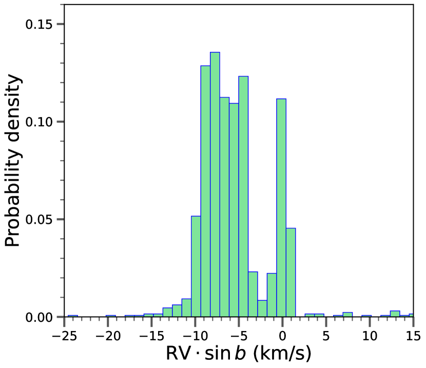
Figure 1: The distribution of the vertical component of radial velocity (${\mathrm{RV}}\cdot\sin b$) obtained from APOGEE; $b$ is the galactic latitude.

We want to emphasize the significance of considering RV in our analysis. As illustrated in Figure 1, when we take into account the YSO sample I and calculate the vertical component of RV using the latitude information of YSOs along with RV data from APOGEE-2, it becomes evident that a substantial portion of the absolute values of the vertical component exceeds the amplitude of $V_{Z}$ oscillations reported in previous studies. Specifically, 62.5$\%$ of the sample exhibit vertical components below $-$5 km/s, which is comparable to the typical value of the weak-amplitude oscillations reported in [29]. This finding underscores the necessity of considering RV.

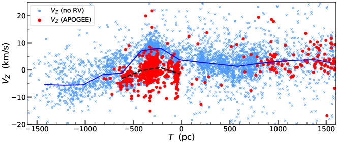
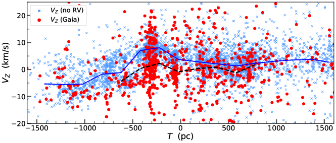
Figure 2: $V_{Z}$ distribution of YSOs along the Radcliffe Wave. The upper panel shows the result using RV data from APOGEE, while the lower panel shows the result using RV data from Gaia. The red points represent more accurate $V_{Z}$ corrected by RV, while the blue points indicate approximate $V_{Z}$ values calculated without considering RV. $T$ represents the direction that the Radcliffe Wave extends, with the zero point on the $T$ axis indicating the closest point to the sun along the Radcliffe Wave. The blue lines represent the median values of blue crosses within 200 pc bins along the $T$ axis, with each bin containing more than 30 points. The black dashed lines represent the median values of the red circles within the same bin.

In the second method, we study molecular clouds directly and extract RV measurements for clouds from the whole-Galaxy CO surveys by [12], which cover the majority of molecular clouds within RW. These comprehensive CO surveys were conducted using the 1.2-meter Millimeter-Wave Telescope at the CfA and its counterpart on Cerro Tololo in Chile. These two instruments have provided the most extensive, uniform, and widely utilized survey of interstellar carbon monoxide (CO) in the Milky Way, serving as the best indicator of the predominantly invisible molecular hydrogen that constitutes the bulk of mass within molecular clouds [42, 11]. From the CO surveys, we get RV measurements of the molecular clouds. However, calculating $V_{Z}$ requires information on the proper motions of the clouds, which are challenging to measure directly and still lacking. Fortunately, there are strong kinematic correlations between the young stellar populations and associated molecular gas and clouds, as reported in [18], [45] and [17]. By considering CO and its isotope molecules as tracers for clouds, there are pieces of evidence supporting that young stars inherit RV from the molecular clouds, as reported in [9, 10]. This suggests a strong relationship between the kinematics of molecular clouds and associated young stars, which implies there is also a similarity in their proper motions. In this approach, we perform a spatial cross-match between the clouds and the associated YSOs in YSO sample II. By doing this, we acquire approximate proper motions for certain molecular clouds. This approximation allows us to calculate $V_{Z}$ for the majority of clouds within RW. To obtain more precise RV and distance measurements for the Cygnus X and North America regions, we also use the data from the MWISP project, referring to 51 for comprehensive information.

By combining RV with the proper motion and location data from Gaia DR3, along with the known component of Solar motion $(U_{\odot},V_{\odot},W_{\odot})=(11.1,12.24,7.25)\,\rm km\,\rm s^{-1}$ [41], we are able to derive the three-dimensional velocities of objects. We also calculate the vertical distance to the Galactic disk based on the precise measurement of the Sun’s position, $Z_{\odot}=20.8\,\rm pc$, from [3].

3 results

3.1 Non-synchronous $V_{Z}$ oscillations

Initially, we utilize RV measurements from APOGEE and Gaia in the first method and obtain more accurate vertical velocities of YSO sample I. These refined $V_{Z}$ are shown with the red data points in Figure 2. In Figure 2, $T$ is the direction RW extends and the zero point on the $T$ axis represents the closest point to the sun along RW (corresponding to the $Y_{\mathrm{prime}}$ axis in the 1). To facilitate comparison, we use blue points to represent the approximate $V_{Z}$ values that were calculated without taking RV measurements into consideration. Additionally, we mark black lines that represent the median values of the blue points within bins of 200 pc along the $T$ axis. We only include bins that contain more than 10 stars in order to ensure statistical significance in our analysis. The upper panel displays the results using RV from APOGEE, while the lower panel shows the results using RV from Gaia. In both panels, the peak of the approximate oscillation (-500 pc¡$T$¡0 pc, corresponding to 0.75 kpc¡$X^{\prime}$¡1.25 kpc in Figure 3 in 29) tends to flatten when RV is taken into account. This suggests that the synchronous oscillation reported in previous studies may arise from the neglect of RV, or at least it should be corrected by incorporating RV measurements.

Figure 3: The spatial and $V_{Z}$ distributions of the cross-matched molecular clouds along the Radcliffe Wave. The matched parts of clouds are depicted as red circles, where the radii represent the relative sizes of the matched parts based on the $T$ axis. The upper panel provides a side view of the spatial distribution, with the red circles indicating the cloud locations and the pink arrows indicating the directions and magnitudes of the $V_{Z}$ component. The length of each arrow corresponds to the value of $V_{Z}$ (in km/s) multiplied by 15. The orange curve marks the fit to the position of the Radcliffe Wave model suggested by [1]. In contrast, locations of the YSOs in YSO sample II are represented by grey points, and the purple ones indicate the cross-matched YSOs. The lower panel displays the distribution of $V_{Z}$. The grey circles and red circles respectively represent the $V_{Z}$ result obtained without and with RV information, accompanied by error bars indicating 1$\sigma$ dispersions.

However, when considering the RV of YSOs, only approximately 20% of the objects have available RV measurements. The coverage of these measurements is primarily on nearby regions such as the Orion, Taurus, and Perseus clouds. However, the coverage of other regions, such as Cygnus X, North America, and the Mon R2 cloud, is inadequate. To gain a more comprehensive understanding, we directly study the molecular clouds as a complementary approach. We utilize the widely recognized whole-galaxy CO surveys conducted by [12] and the data from the MWISP project to obtain RV measurements of these molecular clouds. Subsequently, we combine the proper motions of associated YSOs in YSO sample II, which are highly likely to inherit and preserve the kinematics of their parent clouds. More details of the method is described in Appendix  A. As a result, we obtain the spatial distribution and $V_{Z}$ distribution of the crossed-matched clouds, as illustrated in Figure 3. In Figure 3, the matched parts of molecular clouds are shown with red circles. The size of the circles represents the relative sizes of the matched parts based on the $T$ axis. The upper panel shows a side view of the spatial distribution, where the red circles indicate the locations of the clouds. The pink arrows represent the values of the $V_{Z}$ components. The lower panel displays the distribution of $V_{Z}$ for the clouds, in which the red circles represent the $V_{Z}$ values of clouds obtained by combining RV from the CO surveys and proper motion from associated YSOs, and the grey circles illustrate the results obtained without considering RVs. Our analysis reveals the crucial role of RV measurements in understanding the $V_{Z}$ distribution of RW, particularly in the $T$¡300pc region. Incorporating the RV components leads to a general decrease in the values of $V_{Z}$ in this region.

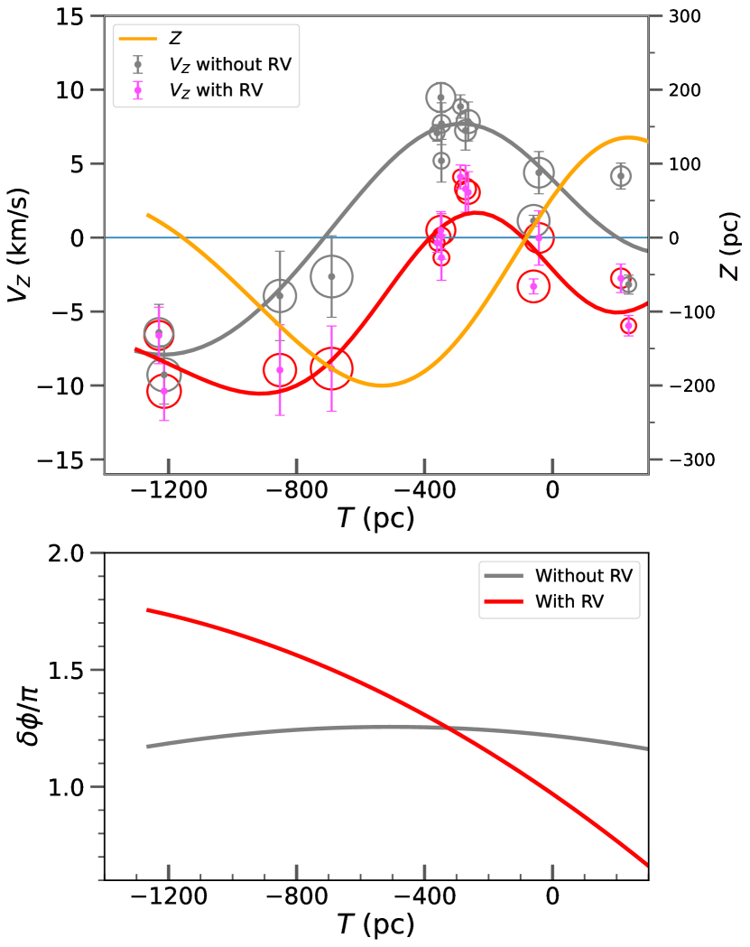
Figure 4: Fitting results of the spatial and $V_{Z}$ distribution of clouds in the $T$¡300 pc region. In the upper panel, the grey line and red line are the fitting results of vertical velocities without and with RV measurements, respectively. The orange line is the fitting result of vertical coordinates (right $y$-axis). The lower panel shows the phase difference ($\delta\phi$) between vertical coordinates and vertical velocities, with the grey and red curves representing the distribution of $\delta\phi$ without and with RV measurements, respectively.

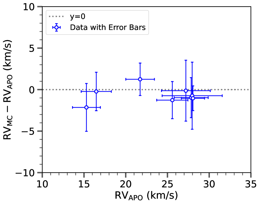
Figure 5: A comparison of RV between clouds and their associated YSOs. Each data point represents a cloud, where the x-axis represents the median RV obtained from APOGGE for the associated YSOs (${\mathrm{RV}}_{\mathrm{APO}}$), and the y-axis represents the residual between the average RV of clouds (${\mathrm{RV}}_{\mathrm{MC}}$) and ${\mathrm{RV}}_{\mathrm{APO}}$. Only the clouds, of which the associated YSOs have RV measurements from APOGEE, are shown in this figure.

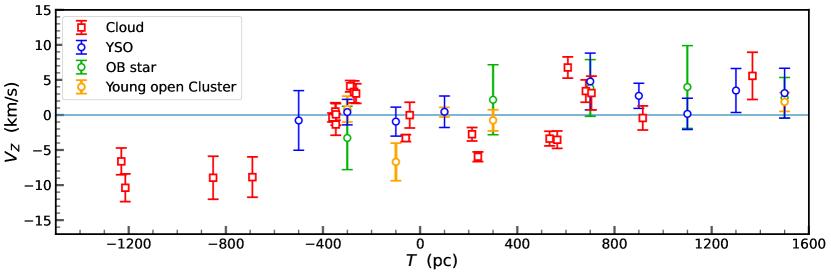
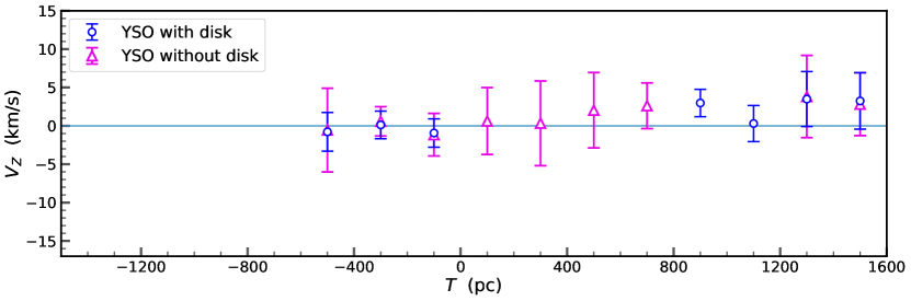
Figure 6: The $V_{Z}$ distribution of clouds (calculated using RV from CO surveys) and young star samples (calculated using RV from APOGEE), with error bars indicating 1$\sigma$ dispersions. The upper panel presents the results of clouds and various young star samples for comparison, including YSO sample II, OB stars, and young open cluster members. For further comparison, the lower panel displays the results for YSOs with and without disks.

In order to investigate the potential presence of synchronous oscillations between $V_{Z}$ and vertical coordinates, we perform separate fitting analyses on $V_{Z}$ without RV and $V_{Z}$ with RV in the $T$¡300 pc region, corresponding to the $X^{\prime}$¡1.55 kpc region as depicted in Figure 3 of [29], where they previously suggested there are synchronous oscillations. In our fitting, we adopt the damped sinusoidal function as proposed by [1] in their equation (1). Figure 4 displays the fitting results for the spatial and $V_{Z}$ distributions of clouds within the $T<300$ pc region. The upper panel of Figure 4 displays curves of different colors representing the fitting results of both the vertical coordinates and the vertical velocities. The grey curve represents the fitting result of the $V_{Z}$ distribution obtained without considering RV measurements. This fitting curve resembles the yellow line shown in Figure 3 of [29]. However, when the RV components are taken into account, as indicated by the red fitting curve, the values of $V_{Z}$ generally decrease in this region. Although a peak still exists in the -500 pc¡$T$¡0 pc region, the red curve exhibits a shorter period and a faster-changing phase compared to the grey curve. In the lower panel of the figure, the phase difference ($\delta\phi$) between the vertical coordinates and the vertical velocities is depicted. When calculated without RV measurements, $\delta\phi$ appears to be constant, similar to the findings reported in [29]. However, when a more precise calculation is performed considering RV measurements, $\delta\phi$ decreases as $T$ increases. These results strongly indicate that the previously reported synchronous oscillation arises due to the neglect of the RV component in previous studies, and there are no synchronous oscillations between vertical coordinates and vertical velocities. Furthermore, separate K-S tests are conducted to evaluate the goodness of fit for the two groups of $V_{Z}$ data, yielding p-values of 0.94 for both tests, which are very close to 1. This indicates excellent fitting performance.

For evaluating the feasibility of this method, we assess the consistency in RVs between the clouds and their associated YSOs. For each successfully matched cloud, we compare its average RV with the median RV of the associated YSOs, which is derived from APOGEE data, as demonstrated in Figure 5. Remarkably, we observe a strong agreement between the two velocities, as evidenced by a maximum absolute residual of only 2.14 km/s and a high correlation coefficient of 0.98. This strong correlation suggests that the method is indeed feasible. It should be noted that our analysis only considers clouds with a minimum of 10 associated YSOs, each having APOGEE RV measurements. This criterion helps mitigate potential random errors that could arise from small sample sizes.

3.2 A $V_{Z}$ dipole pattern without age gradient

Additionally, Figure 3 reveals that the revised vertical velocities demonstrate an overall upward trend as $T$ increases, showing as a dipole in the $V_{Z}$. This trend is similar to the results presented in [44], but with a larger maximum amplitude of approximately 8 km/s.

Moreover, we extend our investigation to explore the $V_{Z}$ distribution of additional star samples along RW, including the OB star sample, the young open cluster member sample, and the Class III YSO sample. In contrast to the study by [44], we incorporate RV measurements by utilizing APOGEE data. Additionally, we use the YSO catalogue from [35] and the catalogues of Class I/II YSOs, and Class III YSOs from [34] for comparative analysis. As a result, Figure 6 depicts the $V_{Z}$ distribution of clouds and young star samples. In Figure 6, we analyze the median vertical velocities of different young samples in bins of 200 pc along the $T$ axis, keeping the bins containing more than 10 stars. In the upper panel, we can observe a consistent overall upward trend in vertical velocities with increasing coordinate $T$, although there are some small oscillations in the intermediate range. This provides a piece of robust evidence for the presence of dipoles in the $V_{Z}$ distribution. For a more in-depth analysis, we incorporate the Class III YSO catalog with YSO sample II in the lower panel and divide this combined sample into two subgroups: YSOs with disks and YSOs without disks. This division is based on the methodology proposed by [48] and [47]. In the lower panel, we also observe the presence of $V_{Z}$ dipoles.

Our findings diverge from those of [44], which observed an age gradient in the oscillation of stars, with the youngest sample exhibiting a maximum dipole. In contrast, our analysis, as depicted in Figure 6, does not provide significant evidence indicating a substantial difference in the size of the dipole between the different samples. Particularly in the lower panel, the younger YSOs that have disks do not exhibit a larger dipole than the older YSOs that do not have disks. These findings suggest that age may not be the primary factor influencing the size of the dipole in $V_{Z}$ among these samples.

4 discussion

4.1 Origin of the non-synchronous oscillation

Different from previous conclusion, we belive that the vertical oscillation in the Radcliffe Wave is non-synchronous. There are two reason. The first is the inclusion of RV measurements. After correcting $V_{Z}$ for RW using two methods, we get a more accurate and comprehensive perspective of the $V_{Z}$ distribution. In contrast to the results that neglect RV components, we observe a general decrease in the values of $V_{Z}$ in the $T$¡300 pc region, while there is little change in other regions. As a result, the phase difference ($\delta\phi$) between the vertical coordinates and the vertical velocities is not consistently constant in this region, contrary to the results reported in [29]. Instead, there is a noticeable decrease in the phase difference along the direction of RW extension ($T$ axis). This suggests that the previous finding of synchronous oscillations in RW was not valid. Part of the reason is our incorporation of the RV component, which has been neglected in previous studies. However, we also note that different authors have adopted different models. It is a combination of these factors which leads to the different conclusions.

4.2 Nature of the dipole pattern

Additionally, the revised $V_{Z}$ consistently demonstrates an upward trend as $T$ increases, revealing dipole patterns in the distribution of $V_{Z}$. Notably, we observe similar dipole patterns when using several young star samples as tracers, which resembles the findings reported in the study by [44], but with a larger amplitude. However, our approach improves upon their results by considering RV measurements from APOGEE-2, while they neglected them. Moreover, contrary to their results, we find no age gradient within the dipole patterns, particularly when comparing the younger YSOs with disks with older YSOs without disks. This suggests that the origin of RW may have comparable effects on both molecular clouds and stars, raising doubts about some formation hypotheses that have a stronger impact on the clouds, such as the Kelvin-Helmholtz instability proposed by [19] and the satellite galaxy perturbations hypothesis proposed by [44]. Currently, the origin of the RW remains a mystery, and our precise and comprehensive analysis of the $V_{Z}$ patterns will contribute to a better understanding and identification of the underlying origin and physical mechanisms involved.

Furthermore, we gain insights into the vertical evolution of RW by considering the influence of the gravitational potential. We approximate the gravitational force in the vertical direction as $F_{Z}$(kg$\cdot$km² s^-2pc^-1)$=-0.003Z$(pc)$\cdot M$(kg), referring to Figure 2 in [40] and [2], where $Z$ represents the vertical distance and $M$ denotes the mass of the cloud. As depicted in Figure 7, RW behaves as an oscillation propagating slowly to the left. It oscillates on the Galactic disk, resembling a harmonic oscillator. The precise $V_{Z}$ information in this article can help to determine the exact amplitude and phase of the oscillation for each cloud. The clouds within RW exhibit similar periods, which can be estimated as t=$2\pi$$\sqrt{\frac{M\times Z}{-F_{Z}}}\approx 110$ Myr. This implies that RW oscillates at such a slow rate that it cannot complete a full period within a cloud’s lifetime, which is estimated to be less than 40 Myr according to [37] and [6]. Additionally, we also investigate the evolution in the X and Y directions and obtain similar results as reported in [31]. RW undergoes significant stretching during the cloud’s lifetime. Combining consideration of the lack of synchronous oscillations between the vertical coordinates and $V_{Z}$, the Radcliffe Wave can hardly be classified as a “wave” in the strict sense.

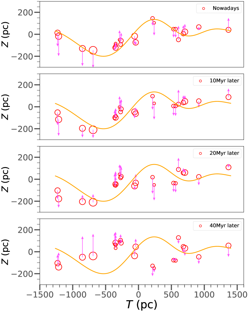
Figure 7: Evolution of the Radcliffe Wave in the vertical direction at different moments: Nowadays, 10 Myr later, 20 Myr later and 40 Myr later. The orange curve marks the current position of RW. The direction of $V_{Z}$ component is represented by pink arrows, with their lengths corresponding to the values of $V_{Z}$ (in km/s) multiplied by 15.

4.3 Future of kinematics studies

To understand the kinematics of RW, it is crucial to have precise measurements of both RV and the proper motion of its gas and cloud members. However, the latter measurements are very uncertain and challenging to define and determine accurately. As a result, using YSOs as tracers may still be a more viable approach. However, the current RV measurements of YSOs are limited to a relatively nearby region and are not comprehensive enough. The upcoming Gaia DR4 and DR5 releases, as well as future RV measurements, will help corroborate the pattern of the vertical oscillations depicted in Figure 3 and Figure 6. By inferring $V_{Z}$ maps of YSOs located near the galactic disk and examining their oscillation patterns, we can obtain valuable insights into the nature of RW.

5 conclusion

We analyze the kinematics of the Radcliffe Wave and find that considering radial velocity measurements is crucial for accurately determining the $V_{Z}$ pattern. By incorporating radial velocity measurements using two methods, we gain a more precise and comprehensive understanding of the distribution of $V_{Z}$. We observe that the oscillations of vertical coordinates and $V_{Z}$ are not synchronized, but exhibit a decreasing phase difference in the $T<300$ pc region (where $T$ corresponds to the $Y_{\mathrm{prime}}$ axis in 1). Furthermore, in the direction along the Radcliffe Wave, $V_{Z}$ shows an upward trend and displays a dipole-like pattern with a maximum amplitude of around 8 km/s. Furthermore, there is no apparent age gradient in the oscillations. Noting that the vertical evolution of the Radcliffe Wave progresses slowly, making it unable to complete a full oscillation within the lifetime of the wave itself, which is around 30 Myr [31], we propose that the Radcliffe Wave does not exhibit typical characteristics of a traditional “wave” in the strict sense.

6 Acknowledgements

This research made use of the data from the Milky Way Imaging Scroll Painting (MWISP) project, which is a multi-line survey in ¹²CO/¹³CO/C¹⁸O along the northern galactic plane with PMO-13.7m telescope. We are grateful to all the members of the MWISP working group, particularly the staff members at PMO-13.7m telescope, for their long-term support. MWISP was sponsored by National Key R$\&$D Program of China with grants 2023YFA1608000 $\&$ 2017YFA0402701 and by CAS Key Research Program of Frontier Sciences with grant QYZDJ-SSW-SLH047. ZJL acknowledges support by the grant AD23026127, funded by Guangxi Science and Technology Project. GXL acknowledges support from NSFC grant No. 12273032 and 12033005. VMP and PP acknowledge financial support by the grant PID2020-115892GB-I00, funded by MCIN/AEI/10.13039/501100011033. This work is supported by the National Natural Science Foundation of China (Grant No.12133003).

Appendix A cross match with CO surveys

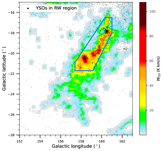
Figure A1: Velocity-integrated spatial CO Map of the Perseus area. YSOs are indicated by black points, marking their respective coordinates within the map. The relatively associated region is marked by the enclosing blue folding frame.

When combining YSO sample II with RV measurements of molecular clouds from the whole-Galaxy CO surveys conducted by [12], our focus is on the regions where YSOs and clouds with higher density (corresponding to larger velocity-integrated intensity of CO—$W_{\mathrm{CO}}$) are associated.

For the spatial cross-matching process, we initially match associated areas in the velocity-integrated spatial ($l$-$b$) CO map based on galactic latitude ($b$) and galactic longitude ($l$). This enables us to identify relatively associated regions, such as the area enclosed by the blue frame depicted in Figure A1 for the Perseus molecular cloud region.

To obtain more accurate RV measurements, we eliminate redundant peaks that may be attributed to overlapping clouds with similar latitude and longitude but at different distances, with reference to previous works, such as [13] for the Perseus molecular cloud area. For other clouds, we also refer to several articles including [32, 28, 14, 26, 49, 50, 10, 15].

Additionally, we determine the distances of the clouds by referring to the compendium provided by [52]. For more accurate RV and distance measurements of Cygnus X and the North America region, we also refer to the data (51) from the MWISP project. Thereafter, we utilize the parallax measurements of YSOs obtained from Gaia DR3. This allows us to refine the distance estimation and effectively eliminate YSOs that are not spatially correlated with the molecular clouds in the radial direction.

Subsequently, we combine RV measurements of the associated cloud areas with the median value of the proper motion measurements of YSOs within the same areas. This combination enables us to calculate the vertical velocities of the clouds.

Appendix B APOGEE vs Gaia

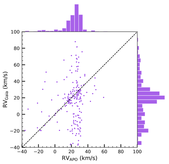
Figure B1: Comparison of radial velocities obtained from Gaia DR3 (${\mathrm{RV}}_{\mathrm{Gaia}}$) and radial velocities obtained from APOGEE-2 (${\mathrm{RV}}_{\mathrm{APO}}$). The black dashed line is the one-to-one line.

In the YSO sample I mentioned in section 2.1, which contains Class I and Class II YSOs along RW, there are 224 YSO members with available RV information from both Gaia DR3 and APOGEE datasets. In Figure B1, we compare the RV measurements from Gaia and APOGEE, where each blue violet point represents a YSO member. The Pearson correlation coefficient ($r$) of the RV values between these two datasets is only 0.10, indicating that the correlation is weak for the sources. In this sample, there is a substantial deviation between RVs obtained from Gaia and APOGEE. Besides, as depicted in Figure B1, RVs from Gaia DR3 exhibit a larger dispersion compared to those from APOGEE. Those two databases exhibit notable differences, emphasizing the need to prioritize the more accurate one for the RVs of young stars. Based on the findings in [25] and [39], which indicate that APOGEE-2 provides more accurate RV measurements for young stars compared to Gaia DR3, we prioritize the results derived from APOGEE in the paper.

References

- Alves et al. [2020] Alves, J., Zucker, C., Goodman, A. A., et al. 2020, Nature, 578, 237, doi: 10.1038/s41586-019-1874-z
- Barros et al. [2016] Barros, D. A., Lépine, J. R. D., & Dias, W. S. 2016, A&A, 593, A108, doi: 10.1051/0004-6361/201527535
- Bennett & Bovy [2019] Bennett, M., & Bovy, J. 2019, MNRAS, 482, 1417, doi: 10.1093/mnras/sty2813
- Blanton et al. [2017] Blanton, M. R., Bershady, M. A., Abolfathi, B., et al. 2017, AJ, 154, 28, doi: 10.3847/1538-3881/aa7567
- Cantat-Gaudin et al. [2020] Cantat-Gaudin, T., Anders, F., Castro-Ginard, A., et al. 2020, A&A, 640, A1, doi: 10.1051/0004-6361/202038192
- Chevance et al. [2023] Chevance, M., Krumholz, M. R., McLeod, A. F., et al. 2023, in Astronomical Society of the Pacific Conference Series, Vol. 534, Protostars and Planets VII, ed. S. Inutsuka, Y. Aikawa, T. Muto, K. Tomida, & M. Tamura, 1, doi: 10.48550/arXiv.2203.09570
- Comerón [1999] Comerón, F. 1999, A&A, 351, 506
- Comeron et al. [1992] Comeron, F., Torra, J., & Gomez, A. E. 1992, Ap&SS, 187, 187, doi: 10.1007/BF00643388
- Da Rio et al. [2016] Da Rio, N., Tan, J. C., Covey, K. R., et al. 2016, ApJ, 818, 59, doi: 10.3847/0004-637X/818/1/59
- Da Rio et al. [2017] —. 2017, ApJ, 845, 105, doi: 10.3847/1538-4357/aa7a5b
- Dame [1993] Dame, T. M. 1993, in American Institute of Physics Conference Series, Vol. 278, Back to the Galaxy, ed. S. S. Holt & F. Verter, 267–278, doi: 10.1063/1.43985
- Dame et al. [2001] Dame, T. M., Hartmann, D., & Thaddeus, P. 2001, ApJ, 547, 792, doi: 10.1086/318388
- Dame & Lada [2023] Dame, T. M., & Lada, C. J. 2023, ApJ, 944, 197, doi: 10.3847/1538-4357/acb438
- Dobashi et al. [1994] Dobashi, K., Bernard, J.-P., Yonekura, Y., & Fukui, Y. 1994, ApJS, 95, 419, doi: 10.1086/192106
- Duan et al. [2023] Duan, Y., Li, D., Pagani, L., et al. 2023, Research in Astronomy and Astrophysics, 23, 095006, doi: 10.1088/1674-4527/acd7bd
- Dunham et al. [2015] Dunham, M. M., Allen, L. E., Evans, Neal J., I., et al. 2015, ApJS, 220, 11, doi: 10.1088/0067-0049/220/1/11
- Fang et al. [2017] Fang, M., Kim, J. S., Pascucci, I., et al. 2017, AJ, 153, 188, doi: 10.3847/1538-3881/aa647b
- Fűrész et al. [2008] Fűrész, G., Hartmann, L. W., Megeath, S. T., Szentgyorgyi, A. H., & Hamden, E. T. 2008, ApJ, 676, 1109, doi: 10.1086/525844
- Fleck [2020] Fleck, R. 2020, Nature, 583, E24, doi: 10.1038/s41586-020-2476-5
- Frogel & Stothers [1977] Frogel, J. A., & Stothers, R. 1977, AJ, 82, 890, doi: 10.1086/112143
- Gaia Collaboration et al. [2016] Gaia Collaboration, Prusti, T., de Bruijne, J. H. J., et al. 2016, A&A, 595, A1, doi: 10.1051/0004-6361/201629272
- Gaia Collaboration et al. [2018] Gaia Collaboration, Brown, A. G. A., Vallenari, A., et al. 2018, A&A, 616, A1, doi: 10.1051/0004-6361/201833051
- Gaia Collaboration et al. [2023] Gaia Collaboration, Vallenari, A., Brown, A. G. A., et al. 2023, A&A, 674, A1, doi: 10.1051/0004-6361/202243940
- Gould [1879] Gould, B. A. 1879, Resultados del Observatorio Nacional Argentino, 1, I
- Kounkel et al. [2023] Kounkel, M., Zari, E., Covey, K., et al. 2023, ApJS, 266, 10, doi: 10.3847/1538-4365/acc106
- Lang et al. [2000] Lang, W. J., Masheder, M. R. W., Dame, T. M., & Thaddeus, P. 2000, A&A, 357, 1001
- Lesh [1972] Lesh, J. R. 1972, A&AS, 5, 129
- Leung & Thaddeus [1992] Leung, H. O., & Thaddeus, P. 1992, ApJS, 81, 267, doi: 10.1086/191693
- Li & Chen [2022] Li, G.-X., & Chen, B.-Q. 2022, MNRAS, 517, L102, doi: 10.1093/mnrasl/slac050
- Li et al. [2013] Li, G.-X., Wyrowski, F., Menten, K., & Belloche, A. 2013, A&A, 559, A34, doi: 10.1051/0004-6361/201322411
- Li et al. [2022] Li, G.-X., Zhou, J.-X., & Chen, B.-Q. 2022, MNRAS, 516, L35, doi: 10.1093/mnrasl/slac076
- Maddalena et al. [1986] Maddalena, R. J., Morris, M., Moskowitz, J., & Thaddeus, P. 1986, ApJ, 303, 375, doi: 10.1086/164083
- Majewski et al. [2017] Majewski, S. R., Schiavon, R. P., Frinchaboy, P. M., et al. 2017, AJ, 154, 94, doi: 10.3847/1538-3881/aa784d
- Marton et al. [2016] Marton, G., Tóth, L. V., Paladini, R., et al. 2016, MNRAS, 458, 3479, doi: 10.1093/mnras/stw398
- McBride et al. [2021] McBride, A., Lingg, R., Kounkel, M., Covey, K., & Hutchinson, B. 2021, AJ, 162, 282, doi: 10.3847/1538-3881/ac2432
- Moreno et al. [1999] Moreno, E., Alfaro, E. J., & Franco, J. 1999, ApJ, 522, 276, doi: 10.1086/307614
- Murray et al. [2010] Murray, N., Quataert, E., & Thompson, T. A. 2010, ApJ, 709, 191, doi: 10.1088/0004-637X/709/1/191
- Pantaleoni González et al. [2021] Pantaleoni González, M., Maíz Apellániz, J., Barbá, R. H., & Reed, B. C. 2021, MNRAS, 504, 2968, doi: 10.1093/mnras/stab688
- Recio-Blanco et al. [2023] Recio-Blanco, A., de Laverny, P., Palicio, P. A., et al. 2023, A&A, 674, A29, doi: 10.1051/0004-6361/202243750
- Sarkar & Jog [2022] Sarkar, S., & Jog, C. J. 2022, A&A, 665, A23, doi: 10.1051/0004-6361/202243184
- Schönrich et al. [2010] Schönrich, R., Binney, J., & Dehnen, W. 2010, MNRAS, 403, 1829, doi: 10.1111/j.1365-2966.2010.16253.x
- Solomon & Barrett [1991] Solomon, P. M., & Barrett, J. W. 1991, in Dynamics of Galaxies and Their Molecular Cloud Distributions, ed. F. Combes & F. Casoli, Vol. 146, 235
- Su et al. [2019] Su, Y., Yang, J., Zhang, S., et al. 2019, ApJS, 240, 9, doi: 10.3847/1538-4365/aaf1c8
- Thulasidharan et al. [2022] Thulasidharan, L., D’Onghia, E., Poggio, E., et al. 2022, A&A, 660, L12, doi: 10.1051/0004-6361/202142899
- Tobin et al. [2015] Tobin, J. J., Hartmann, L., Fűrész, G., Hsu, W.-H., & Mateo, M. 2015, AJ, 149, 119, doi: 10.1088/0004-6256/149/4/119
- Tu et al. [2022] Tu, A. J., Zucker, C., Speagle, J. S., et al. 2022, ApJ, 936, 57, doi: 10.3847/1538-4357/ac82f0
- Wang & Chen [2019] Wang, S., & Chen, X. 2019, ApJ, 877, 116, doi: 10.3847/1538-4357/ab1c61
- Wang et al. [2022] Wang, X.-L., Fang, M., Gao, Y., et al. 2022, ApJ, 936, 23, doi: 10.3847/1538-4357/ac8426
- Wilson et al. [2005] Wilson, B. A., Dame, T. M., Masheder, M. R. W., & Thaddeus, P. 2005, A&A, 430, 523, doi: 10.1051/0004-6361:20035943
- Xu et al. [2013] Xu, Y., Li, J. J., Reid, M. J., et al. 2013, ApJ, 769, 15, doi: 10.1088/0004-637X/769/1/15
- Zhang et al. [2024] Zhang, S., Su, Y., Chen, X., et al. 2024, ApJS
- Zucker et al. [2020] Zucker, C., Speagle, J. S., Schlafly, E. F., et al. 2020, A&A, 633, A51, doi: 10.1051/0004-6361/201936145
- Zucker et al. [2022] Zucker, C., Goodman, A. A., Alves, J., et al. 2022, Nature, 601, 334, doi: 10.1038/s41586-021-04286-5