Ranking Entities along Conceptual Space Dimensions with LLMs:
An Analysis of Fine-Tuning Strategies

Abstract

Conceptual spaces represent entities in terms of their primitive semantic features. Such representations are highly valuable but they are notoriously difficult to learn, especially when it comes to modelling perceptual and subjective features. Distilling conceptual spaces from Large Language Models (LLMs) has recently emerged as a promising strategy. However, existing work has been limited to probing pre-trained LLMs using relatively simple zero-shot strategies. We focus in particular on the task of ranking entities according to a given conceptual space dimension. Unfortunately, we cannot directly fine-tune LLMs on this task, because ground truth rankings for conceptual space dimensions are rare. We therefore use more readily available features as training data and analyse whether the ranking capabilities of the resulting models transfer to perceptual and subjective features. We find that this is indeed the case, to some extent, but having perceptual and subjective features in the training data seems essential for achieving the best results. We furthermore find that pointwise ranking strategies are competitive against pairwise approaches, in defiance of common wisdom.

Ranking Entities along Conceptual Space Dimensions with LLMs:
An Analysis of Fine-Tuning Strategies

Nitesh Kumar  and Usashi Chatterjee  and Steven Schockaert Cardiff NLP, School of Computer Science and Informatics Cardiff University, United Kingdom {kumarn8,chatterjeeu,schockaerts1}@cardiff.ac.uk

1 Introduction

Knowledge graphs (KGs) have emerged as the de facto standard for representing knowledge in areas such as Natural Language Processing Schneider et al. (2022), Recommendation Guo et al. (2022) and Search Reinanda et al. (2020). However, much of the knowledge that is needed in applications is about graded properties, e.g. recipes being healthy, movies being original or cities being kids-friendly. Such knowledge is easiest to model in terms of rankings: we can rank recipes according to how healthy they are even if we cannot make a hard decision about which ones are healthy and which ones are not. For this reason, we argue that conceptual spaces Gärdenfors (2000) should be used, alongside knowledge graphs, in many settings.

A conceptual space specifies a set of quality dimensions, which correspond to primitive semantic features. For instance, in a conceptual space of movies, we might have a quality dimensions reflecting how original a movie is. Entities are represented as vectors, specifying a suitable feature value for each quality dimension. While the framework of conceptual spaces is more general, we will essentially view quality dimensions as rankings.

Conceptual spaces have the potential to play a central role in various knowledge-intensive applications. In the context of recommendation, for instance, they could clearly complement the factual knowledge that is captured by typical KGs (e.g. modelling the style of a movie, rather than who directed it), making it easier to infer user preferences from previous ratings. They could also be used to make recommendations more controllable, as in the case of critiquing-based systems, allowing users to specify feedback of the form “like this movie, but more kids-friendly” Chen and Pu (2012); Vig et al. (2012). Conceptual spaces furthermore serve as a natural interface between neural and symbolic representations Aisbett and Gibbon (2001), and may thus enable principled explainable AI methods.

However, the task of learning conceptual spaces has proven remarkably challenging. The issue of reporting bias Gordon and Durme (2013), in particular, has been regarded as a fundamental obstacle: the knowledge captured by conceptual spaces is often so obvious to humans that it is rarely stated in text. For instance, the phrase “green banana” is more frequent in text than “yellow banana” Paik et al. (2021), as the colour is typically not specified when yellow bananas are discussed. Paik et al. (2021) found that predictions of Language Models (LMs) about the colour of objects were correlated with the distribution of colour terms in text corpora, rather than with human judgements, suggesting that LMs cannot overcome the challenges posed by reporting bias. However, Liu et al. (2022a) found that larger LMs can perform much better on this task. Going beyond colour, Chatterjee et al. (2023) evaluated the ability of LLMs to predict taste-related features, such as sweetness and saltiness, obtaining mixed results: the rankings predicted by LLMs, in a zero-shot setting, had a reasonable correlation with human judgments but they were not consistently better than those produced by a fine-tuned BERT Devlin et al. (2019) model.

In this paper, we analyse whether LLMs can be fine-tuned to extract better conceptual space representations. The difficulty is that ground truth rankings are typically not available when it comes to perceptual and subjective features, outside a few notable exceptions such as the aforementioned taste dataset. We therefore explore whether more readily available features can be used for fine-tuning the model. For instance, we can obtain ground truth rankings from Wikidata entities with numerical attributes (e.g. the length of rivers, the birth date of people, or the population of cities) and then use these rankings to fine-tune an LLM. We furthermore compare two different strategies for ranking entities with an LLM: the pointwise approach uses an LLM to assign a score to each entity, given some feature, while the pairwise approach uses an LLM to decide which among two given entities has the feature to the greatest extent. Our contributions and findings can be summarised as follows:

• We evaluate on three datasets which have not previously been used for studying language models: a dataset of rocks, a dataset of movies and books, and a dataset about Wikidata entities. We use these datasets alongside datasets about taste Chatterjee et al. (2023) and physical properties Li et al. (2023).

• We analyse whether fine-tuning LLMs on features from one domain (e.g. taste) can improve their ability to rank entities in different domains (e.g. rocks). We find this indeed largely to be the case, as long as the training data also contains perceptual or subjective features.

• We compare pointwise and pairwise approaches for ranking entities with LLMs. Despite the fact that pairwise approaches have consistently been found superior for LLM-based document ranking Nogueira et al. (2019); Gienapp et al. (2022); Qin et al. (2023), when it comes to ranking entities, we find the pointwise approach to be highly effective.

• To obtain rankings from pairwise judgments, we need a suitable strategy for aggregating these judgments. We show the effectiveness of an SVM based strategy for this purpose. While this strategy is known to have desirable theoretical properties, it has not previously been considered in the context of language models, to the best of our knowledge

2 Related Work

LMs as Knowledge Bases

Our focus in this paper is on extracting knowledge from language models. This idea of language models as knowledge bases was popularised by Petroni et al. (2019), who showed that the pre-trained BERT model captures various forms of factual knowledge, which can moreover be extracted using a simple prompt. Work in this area has focused on two rather distinct goals. On the one hand, probing tasks, such as the one proposed by Petroni et al. (2019), have been used as a mechanism for analysing and comparing different language models. On the other hand, extracting knowledge from LMs has also been studied as a practical tool for building or extending symbolic knowledge bases. This has been particularly popular for capturing types of knowledge which are not commonly found in traditional knowledge bases, such as commonsense knowledge Bosselut et al. (2019); West et al. (2022); Yu et al. (2023). Several works have focused on distilling KGs from language models Cohen et al. (2023). Hao et al. (2023) studies this problem for non-traditional relations such as “is capable of but not good at”. Along the same lines, Ushio et al. (2023) have focused on modelling relations that are a matter of degree, such as “is a competitor of” or “is similar to”. We can similarly think of the conceptual space dimensions that we consider in this paper as gradual properties.

Where the aforementioned approaches explicitly extract knowledge from an LM, the knowledge captured by LMs has also been used implicitly, by applying such models in a wide range of knowledge-intensive applications, including closed-book question answering Roberts et al. (2020), knowledge graph completion Yao et al. (2019), recommendation Sun et al. (2019); Geng et al. (2022), entity typing Huang et al. (2022) and ontology alignment He et al. (2022), to name just a few.

Conceptual Space of LMs

There is an ongoing debate about the extent to which LMs can truly capture meaning Bender and Koller (2020); Abdou et al. (2021); Patel and Pavlick (2022); Søgaard (2023). Within this context, several authors have analysed the ability of LMs to predict perceptual features. As already mentioned, Paik et al. (2021) and Liu et al. (2022a) analysed the ability of LMs to predict colour terms. Abdou et al. (2021) analyses whether the representation of colour terms in LMs can be aligned with their representation in the CIELAB colour space. Patel and Pavlick (2022) similarly showed that LLMs can generate colour terms from RGB codes in a few-shot setting, even if the codes represent a rotation of the standard RGB space. They also show a similar result for terms describing spatial relations. Zhu et al. (2024) have similarly shown that LLMs can understand colour codes, by using them to generate HSL codes for everyday objects, or by asking models to choose the most suitable code among two alternatives.

Beyond the colour domain, Li et al. (2023) considered physical properties such as height or mass. While they found LLMs to struggle with such properties, Chatterjee et al. (2023) reported better results on the same datasets, especially for GPT-4. Focusing on visual features, Merullo et al. (2023) showed that the representations of concepts in vision-only and text-only models can be aligned using a linear mapping. Chatterjee et al. (2023) focused on the taste domain, modelling properties such as sweet. They found that GPT-3 can model such properties to a reasonable extent, but not better than a fine-tuned BERT model.

Gupta et al. (2015) already considered the problem of modelling gradual properties in the context of static word embeddings, although their analysis was limited to objective numerical features. Derrac and Schockaert (2015) similarly learned conceptual space dimensions for properties such as “violent” in a semantic space of movies. These approaches essentially learn a linear classifier or regression model for each property indepdently, and can thus not generalise to new properties.

3 Extracting Rankings

We consider the following problem: given a set of entities $\mathcal{E}$ and a feature $f$, rank the entities in $\mathcal{E}$ according to the their value for the feature $f$. In some cases, $f$ will refer to a numerical attribute. For instance, $\mathcal{E}$ may be a set of countries and $f$ the population of a country, where the task is then to rank the countries according to their population. In other cases, $f$ will rather refer to a gradual property. For instance, $\mathcal{E}$ may be a set of food items and $f$ may be the level of sweetness. Let us write $f(e)$ for the value of feature $f$ for entity $e$.

We consider two broad strategies for solving the considered ranking task with LLMs. First, we can use LLMs to map each entity $e$ to some score $w(e)$, with the assumption that $w(e_{1})<w(e_{2})$ iff $f(e_{1})<f(e_{2})$. This pointwise approach to learning to rank is considered in Section 3.2. Second, we can use LLMs to solve a binary classification problem: given two entities $e_{1}$ and $e_{2}$, decide whether $f(e_{1})<f(e_{2})$ holds. This pairwise approach needs to be combined with a strategy for aggregating the LLM predictions into a single ranking. The main disadvantage is that a large number of judgements need to be collected for this to be effective, which means that such approaches are less efficient than pointwise strategies. However, in the context of document retrieval, pairwise approaches have been found to outperform pointwise approaches Nogueira et al. (2019); Gienapp et al. (2022); Qin et al. (2023). We discuss pairwise and pointwise strategies in Sections 3.1 and 3.2 respectively. Finally, Section 3.3 describes how we establish baseline results using ChatGPT and GPT4.

3.1 Pairwise Model

The problem of predicting whether $f(e_{1})<f(e_{2})$ holds can be straightforwardly cast as a sequence classification problem. To this end, we use a prompt of the following form:

• This question is about two [entity type]: [Is/Does/Was] [entity 1] [comparative feature] than [entity 2]?

Note that the exact formulation depends on the type of feature which is used for ranking. For instance, some instantiations of the prompt are as follows:

• This question is about two rivers: Is River Thames longer than Seine?

• This question is about two companies: Was Meta founded after Alphabet?

• This question is about two food items: Does banana taste sweeter than chicken?

In initial experiments, we used prompts with a more uniform style (e.g. “should [entity 1] be ranked higher than [entity 2] in terms of [feature]”). However, this inevitably leads to less natural sounding prompts for certain features, which may affect performance. Moreover, such prompts were sometimes found to be ambiguous (e.g. does “ranked higher in terms of date of birth” mean younger people should be ranked highest?). To obtain judgments about entity pairs, we use a standard sequence classification approach, where a linear layer with sigmoid activation is applied to the final hidden state. The model is trained using binary cross entropy using a set of training examples.

Aggregating judgments

We typically want to rank a given set of entities, rather than judging the relative position of two particular elements. This means that we need a strategy for aggregating (noisy) pairwise judgments into a single ranking. This problem has received extensive attention in the literature, with standard techniques including spectral ranking Vigna (2016) and maximum likelihood estimation w.r.t. an underlying statistical model. However, existing approaches often consider a stochastic setting, where we may have access to several judgments for the same entity pair (e.g. when ranking sports teams based on the outcomes of head-to-head matches).

Our setting is slightly different, as we can realistically only obtain judgments for a small sample of entity pairs. In particular, we ideally need methods with $\Omega(n)$ sample complexity, i.e. methods that can perform well with a number of judgements that is linear in the number of queries. Wauthier et al. (2013) discuss two such methods. Let us write $e_{1},...,e_{n}$ for the entities to be ranked. The first method uses a linear SVM to learn a weight vector $\mathbf{w}=(w_{1},...,w_{n})$. Let $\mathbf{x}_{i}$ be an $n$-dimensional one-hot vector, which is $1$ in the $i$^th coordinate and 0 elsewhere. If we have a pairwise judgement $f(e_{i})<f(e_{j})$ then this is translated into the constraint that $\mathbf{w}(\mathbf{x}_{j}-\mathbf{x}_{i})>0$. A standard SVM can then be used to find the vector $\mathbf{w}$ that maximises the margin between positive and negative examples. Entity $e_{i}$ is ranked based on its corresponding weight $w_{i}$. The second method simply scores each entity $e_{i}$ based on the number of pairwise comparisons where $e_{i}$ was ranked higher/lower. Specifically, let us define $s_{ij}=1$ if entities $e_{i}$ and $e_{j}$ have been compared, and $s_{ij}=0$ otherwise. Furthermore, we define $c_{ij}=1$ if $f(e_{i})>f(e_{j})$, according to a pairwise comparison that was made, and $c_{ij}=-1$ otherwise. Then we can choose the weights as:

$$w_{i}=\frac{\sum_{j\neq i}s_{ij}c_{ij}}{\sum_{j\neq i}s_{ij}}$$

We will refer to this strategy as Count.

3.2 Pointwise Model

For the pointwise model, we need to learn a scoring function $w:\mathcal{E}\rightarrow\mathbb{R}$. To this end, we use a prompt of the following form:

• Is [entity 1] among [superlative feature] [entity type]?

For instance, Is River Thames among the longest rivers? For each entity $e_{i}$, we obtain a score $w(e_{i})\in\mathbb{R}$ by applying a linear layer to the final hidden state. Intuitively, $w(e_{i})$ captures the (latent) quality of $e_{i}$ w.r.t. the considered feature. Since we cannot obtain ground truth labels for this score, we again rely on pairwise comparisons for training the model. Specifically, we estimate the probability $p_{ij}$ that $f(e_{i})>f(e_{j})$ holds as:

$$p_{ij}=\sigma\big{(}w(e_{i})-w(e_{j})\big{)}$$

Then we use binary cross entropy as follows:

$$\mathcal{L}=-\Big{(}\sum_{i\neq j}t_{ij}\log p_{ij}+(1-t_{ij})\log(1-p_{ij})\Big{)}$$

where $t_{ij}=1$ if $f(e_{i})>f(e_{j})$ and $t_{ij}=0$ otherwise, and the summation ranges over all distinct entity pairs $e_{i},e_{j}$ within the given mini-batch. Note that while we use pairwise comparisons for training the model, it is still a pointwise approach as it produces scores for individual entities.

3.3 Baselines

To put the performance of the fine-tuning strategies from Sections 3.1 and 3.2 into context, we compare them with two conversational models: ChatGPT (gpt-3.5-turbo) and GPT-4 (gpt-4). We use both models in a zero-shot setting. For this purpose, we use the same prompt as in Section 3.1 but append the sentence Only answer with yes or no. Despite this instruction, the models occasionally still generates a different response, typically expressing that the question cannot be answered. For such entity pairs, we replace the generated response with a randomly generated label (yes or no).

4 Datasets

In our experiments, we will rely on the following datasets, either for training or for testing the models. Each dataset consists of a number of rankings, where each ranking is defined by a set of entities and a feature along which the entities are ranked.

Wikidata

We have obtained 20 rankings from numerical features that are available on Wikidata. For instance, we obtained a ranking of rivers by comparing their length.. If there were more than 1000 entities with a given feature value, we selected the most 1000 popular entities. To estimate the popularity of an entity, we use their QRank, which counts the number page views of the corresponding entry in sources such as Wikipedia. For the entity type person, we limited the analysis to people born in London (which made it possible to retrieve the required information from Wikidata more efficiently). We similarly only considered museums located in Italy. For some experiments, we split the collected data in two datasets, called WD1 and WD2. This will allow us to test whether models trained on one set of features (i.e. WD1) generalise to a different set of feature (i.e. WD2). WD1 contains rankings which were cut off at 1000 elements, whereas WD2 contains rankings with fewer elements. We will write WD to refer to the full dataset, i.e. WD1 and WD2 combined.

	Wikidata		Taste						Rocks							TG		Phys
	WD1-test	WD2	Sweetness	Saltiness	Sourness	Bitterness	Umaminess	Fattiness	Lightness	Grain size	Roughness	Shininess	Organisation	Variability	Density	Movies	Books	Size	Height	Mass	Average
Pointwise
Llama2-7B	80.5	61.0	62.8	53.2	47.2	52.6	58.2	65.0	62.0	60.2	56.4	42.0	53.6	61.2	72.2	59.3	52.8	68.0	70.0	50.0	59.4
Llama2-13B	79.8	58.7	52.8	70.4	51.2	52.8	65.2	67.2	66.4	49.6	43.2	52.6	57.0	57.2	65.2	60.9	55.0	69.6	76.4	58.4	60.5
Mistral-7B	78.3	61.4	70.2	69.4	64.8	59.2	67.8	68.8	61.0	57.4	42.4	47.8	61.0	52.4	56.0	62.4	59.3	85.6	70.0	61.0	62.8
Pairwise
Llama2-7B	81.8	61.6	59.0	59.8	52.0	53.8	60.8	61.8	50.8	62.6	52.2	46.6	56.0	55.8	64.4	57.0	60.1	86.2	81.2	68.0	61.6
Llama2-13B	82.8	68.0	58.6	67.4	50.8	53.6	67.6	67.6	50.2	66.8	58.4	52.0	55.8	58.8	68.8	58.3	55.6	93.8	91.2	66.2	64.6
Mistral-7B	82.2	64.2	59.4	69.0	52.4	52.4	66.8	63.0	58.6	55.0	52.6	47.8	54.8	52.0	58.8	53.3	52.3	92.6	88.0	68.2	62.2
Baselines
ChatGPT	55.3	60.9	60.4	58.4	52.4	51.0	53.2	54.2	60.4	60.2	57.0	51.4	53.2	55.2	62.8	63.8	67.2	77.8	70.8	58.6	59.2
GPT-4	77.2	78.3	76.6	80.6	62.6	56.2	69.2	73.8	72.8	70.2	56.6	62.4	59.4	63.6	74.0	67.4	66.9	99.2	95.2	64.0	71.3

Table 1: Comparison of different models in terms of accuracy ($\%$), when classifying pairwise judgments. The pointwise and pairwise models are trained on the training split of WD1.

	Wikidata		Taste						Rocks							TG		Phys
	WD1-test	WD2	Sweetness	Saltiness	Sourness	Bitterness	Umaminess	Fattiness	Lightness	Grain size	Roughness	Shininess	Organisation	Variability	Density	Movies	Books	Size	Height	Mass
WD1-train	82.8	68.0	58.6	67.4	50.8	53.6	67.6	67.6	50.2	66.8	58.4	52.0	55.8	58.8	68.8	58.3	55.6	93.8	91.2	66.2
WD	-	-	55.2	64.8	51.2	53.8	62.4	63.0	46.8	68.8	60.8	60.0	50.4	64.8	70.6	65.3	62.3	78.0	79.4	60.4
TG	63.3	56.9	71.2	71.6	60.0	58.8	69.0	65.6	71.2	69.6	48.8	60.6	57.6	55.8	66.0	-	-	50.6	54.6	55.2
Taste	62.1	51.1	-	-	-	-	-	-	66.4	72.2	56.8	60.8	58.6	53.2	74.0	66.2	55.7	53.0	61.4	58.2
WD+TG+Taste	-	-	-	-	-	-	-	-	61.2	70.6	57.0	59.2	62.8	57.6	78.4	-	-	77.8	85.4	62.2
WD+TG+Rocks	-	-	74.0	72.4	60.0	60.2	70.6	72.2	-	-	-	-	-	-	-	-	-	85.6	88.2	62.0
WD+Taste+Rocks	-	-	-	-	-	-	-	-	-	-	-	-	-	-	-	69.1	65.2	89.4	91.2	63.8

Table 2: Comparison of different models in terms of accuracy ($\%$), when classifying pairwise judgments. All results are for the pairwise model with Llama2-13B.

Taste

Following Chatterjee et al. (2023), we use a dataset with ratings about the taste of 590 food items along six dimensions: sweetness, sourness, saltiness, bitterness, fattiness and umaminess. The dataset was created by Martin et al. (2014), who used a panel of twelve experienced food assessors to rate the items. We use the version of the dataset that was cleaned by Chatterjee et al. (2023), who altered some of the descriptions of the items to make them sound more natural in prompts.

Rocks

Nosofsky et al. (2018) created a dataset of rocks, with the aim of studying how cognitively meaningful representation spaces for complex domains can be learned. A total of 30 rock types were studied (10 igneous rocks, 10 metamorphic rocks and 10 sedimentary rocks). For each type of rock, 12 pictures were obtained, and each picture was annotated along 18 dimensions. However, only 7 of the considered dimensions allow for ranking all types: lightness of colour, average grain size, roughness, shininess, organisation, variability of colour and density. For our experiments, we only considered these dimensions. The dataset from Nosofsky et al. (2018) contains ratings for each of the 12 pictures of a given rock type, where each picture was assessed by 20 annotators. To construct rankings of rock types, we average the ratings across the 12 pictures. As such, we end up with 7 rankings of 30 rock types.

Tag Genome

Vig et al. (2012) collected a dataset of movies, called the Tag Genome, by asking annotators to what extent different tags apply to different movies, on a scale from 1 to 5. From these tags, we first selected those that correspond to adjectives and for which ratings for at least 15 movies were available. We then manually identified 38 of these adjectives which correspond to ordinal features. More recently, Kotkov et al. (2022) created a similar dataset for books. We again selected adjectives for which at least 15 items were ranked, and manually identified 32 adjectives that correspond to ordinal features. A list of the adjectives that we considered, together with the corresponding number of items in the rankings, is provided in the appendix. It should be noted that most items are only judged by a single annotator, and the judgements were moreover obtained using crowdsourcing. The movies and books datasets are thus clearly noisier than the taste and rocks datasets. By averaging across a large number of rankings, we believe that these datasets can nonetheless be valuable. For this reason, we will only consider aggregated results across all tags when evaluating on these datasets. We will write TG to refer to the combined dataset, containing both the books and movies rankings.

Physical Properties

Following Li et al. (2023), we consider three physical properties: mass, size and height. The ground truth for mass dataset was obtained from a dataset about household objects from Standley et al. (2017). Following Chatterjee et al. (2023), we removed 7 items, because their mass cannot be assessed without the associated image: big elephant, small elephant, Ivan’s phone, Ollie the monkey, Marshy the elephant, boy doll and Dali Clock. The resulting dataset has 49 items. For size and height, we use the datasets from Liu et al. (2022b) as ground truth. These datasets each consist of 500 pairwise judgements.

	Sweetness	Saltiness	Sourness	Bitterness	Umaminess	Fattiness
Pointwise	51.0	64.8	32.5	35.2	52.0	61.7
SVM (5 samples)	62.1	62.2	42.6	44.6	56.4	63.0
SVM (30 samples)	66.0	64.7	47.6	47.0	60.6	65.8
Count (5 samples)	59.0	57.4	46.7	41.7	53.5	60.1
Count (30 samples)	64.8	64.7	49.1	47.2	59.9	64.7
Ada∗	17.5	8.5	12.2	16.4	22.5	10.7
Babbage∗	19.5	51.1	20.2	22.0	22.6	16.0
Curie∗	36.0	46.3	32.8	23.2	22.6	31.7
Davinci∗	55.0	63.2	33.3	27.2	57.0	52.0

Table 3: Comparison of ranking strategies, in terms of Spearman $\rho$%. Baseline results marked with ^∗ were taken from Chatterjee et al. (2023). All other results are obtained with Llama-13B trained on WD+TG+Rocks.

Feature	Top ranked entities	Bottom ranked entities
Sweetness	mango, dried date, white chocolate, peach , pineapple in syrup, fruit candy, syrup with water, ice cream, strawberry, sweet pancake with maple syrup	minced beef patty, grilled calf livers, squid, sandwich with cold cuts, gizzards, croque-monsieur, roast rabbit, stir-fried bacon, roast beef , calf head with vinaigrette
Saltiness	green olives, extruded salty crackers, soy sprouts with soy sauce, canned anchovies, canned sardines, pasta with soy sauce, salted pies, marinated mussels, potato chips, salted cake	clafoutis, raspberry cake, stewed apple, raspberry with whipped cream, white chocolate, strawberry with cream and sugar, mix fruits juice, apple, raspberry, strawberry
Scary	Descent, The (2005), Grudge, The (2004), Exorcist, The (1973), Silence of the Lambs, The (1991), Ring, The (2002), Texas Chainsaw Massacre, The (1974), Shining, The (1980), Seven (a.k.a. Se7en) (1995), Amityville Horror, The (2005), American Werewolf in London, An (1981)	Super Size Me (2004), Station Agent, The (2003), Ray (2004), Dances with Wolves (1990), Jerry Maguire (1996), Driving Miss Daisy (1989), School of Rock (2003), Kung Fu Panda (2008), Miss Congeniality (2000), Ninotchka (1939)
Funny	Ace Ventura: When Nature Calls (1995), Ace Ventura: Pet Detective (1994), Hot Shots! Part Deux (1993), Army of Darkness (1993), South Park: Bigger, Longer and Uncut (1999), Auntie Mame (1958), Blazing Saddles (1974), Clerks (1994), Grand Day Out with Wallace and Gromit, A (1989), Hitchhiker’s Guide to the Galaxy, The (2005)	Spanish Prisoner, The (1997), Son of Dracula (1943), Ghost Dog: The Way of the Samurai (1999), Ferngully: The Last Rainforest (1992), High Crimes (2002), Cadillac Man (1990), Bad Boys II (2003), House of Wax (1953), Fire in the Sky (1993), Step Up 2 the Streets (2008)
Population	India, Nigeria, People’s Republic of China, Iran, Pakistan, United States of America, Russia, Indonesia, Egypt, Bangladesh	Dominica, Nauru, Andorra, Cook Islands, Saint Vincent and the Grenadines, Seychelles, Palau, Northern Mariana Islands, Liechtenstein, Niue

Table 4: We show the top and bottom ranked entities for five features: sweetness and saltiness, from the food dataset, scary and funny, from movies, and countries population, from WD2.

5 Experiments

We now evaluate the performance of the fine-tuning strategies on the considered datasets.

Comparing Models

Table 1 compares a number of different models. We test three different LLMs: the 7B and 13B parameter Llama 2 models and the 7B parameter Mistral model. We evaluate the different models in terms of their accuracy on pairwise judgements. To this end, for a given dataset, we randomly sample pairs of entities $e_{i},e_{j}$ and construct queries asking whether $f(e_{i})>f(e_{j})$. For WD, Taste and Rocks, we sample 500 such pairs for each of the features. Since the TG dataset has a total of 70 features, we limit the test set to 100 pairs per feature. For this analysis, we have split the WD1 dataset into two parts: 80% of the entities, for each feature, are used for training the models. The remaining 20% are used as a test set. All models are fine-tuned on the training split of WD1 (apart from the baselines, which are evaluated zero-shot). This allows us to see how well the models perform on the features they were trained on (by evaluating on the WD1 test split), as well as how they generalise to unseen properties.

The aim of the analysis in Table 1 is to assess whether models can be successfully fine-tuned using a relatively small training set (i.e. WD1-train), involving only well-defined numerical features. In particular, we want to test whether models which are fine-tuned on such features would also generalise to more subjective and less readily available ones, similar to the easy-to-hard generalisation that has been observed for LLMs in other tasks Hase et al. (2024). The results show that this is only the case to some extent. Overall, we can see that Mistral-7B achieves the best results among the pointwise models, while Llama2-13B achieves the best results among the pairwise models. The performance of the pointwise Mistral-7B model is particularly surprising, given that pairwise models generally perform better in ranking tasks. The performance of the models across different features is not always consistent. Each model achieves close to random chance on some of the features, but the features where one model performs poorly are not always the same features where other models perform poorly. However, for bitterness and roughness, all models perform below 60% F1. Furthermore, sourness and organisation also stand out as being more challenging. Regarding the baselines, GPT-4 generally performs better than the fine-tuned models. ChatGPT performs worse on most features, but achieves the best results for books.

Comparing Training Sets

The relatively disappointing results from Table 1 can be partially explained by the fact that a small training set was used, which moreover only covered numerical features and particular entity types. In Table 2, we evaluate the impact of using different training sets. For this analysis, we use the pairwise Llama2-13B model. Our focus is on seeing whether models trained on one domain can generalise to other domains. The results are again evaluated in terms of accuracy, using the same pairwise judgements as for Table 1. WD refers to the full dataset (including both the training and test splits of WD-1).

We can see that training on larger datasets indeed leads to considerably better results. While this is not unexpected, we can also make more striking observations in Table 2. For instance, the model that was trained on Taste alone achieves strong results on Rocks, despite the two datasets involving very different features. Similarly, the model that was only trained on TG achieves strong results for both Taste and Rocks. This suggests that the fine-tuned models are indeed capable of generalising to unseen domains. However, to achieve strong results, it appears to be important that the training data contains subjective or perceptual features. Indeed, training on TG alone overall performed poorly, compared to the other training sets. The best results in Table 2 are competitive with the GPT-4 results from Table 1. Given that the training and test sets cover disjoint domains, the results in Table 2 reflect the knowledge that is captured by the LLMs themselves, rather than knowledge that was injected during the fine-tuning process. This suggests that pre-trained LLMs capture more perceptual knowledge than it may initially appear.

Comparing Ranking Strategies

Table 3 compares different strategies for generating rankings. The pointwise model can be used directly for this purpose. For the pairwise model, we show results with the SVM strategy and the Count strategy. For Count, we furthermore vary the number of pairwise judgments per entity (5 or 30). For this experiment, we use the (pointwise and pairwise) Llama2-13B models that were trained on WD+TG+Rocks. We evaluate the different models by comparing the predicted rankings with the ground truth in terms of Spearman $\rho$. We can see that the pairwise approaches outperform the pointwise model in this case. This is somewhat surprising, given the strong performance of the pointwise models in Table 1. Essentially, because the ranking strategies aggregate many pairwise samples, the noisy nature of the pairwise judgments can to some extent be mitigated. The SVM method generally performs better than the Count method, especially in the case where only 5 judgments per entity are obtained. We also compare with the GPT-3 results reported by Chatterjee et al. (2023), finding that the pairwise Llama model consistently performs best.

Qualitative Analysis

Table 4 shows the 10 highest and lowest ranked entities, according to the rankings from the SVM method with the pairwise Llama2-13B model. The results for sweetness and saltiness were obtained with the model that was trained on WD+TG+Rocks. The rankings for scary and funny movies were obtained with the model that was trained on WD+Taste+Rocks. The ranking for population was obtained with the model that was trained on WD1. The table shows that the model was successful in selecting these top and bottom ranked entities. The top-ranked entities for sweetness, for instance, are all clearly sweet food items, while none of the bottom ranked entities are. Similar observations can be made for the other features. The model is sometimes less successful in distinguishing middle-ranked entities from bottom-ranked entities. For instance, most cheeses appear at the bottom of the ground truth ranking, whereas the model predicted these to be somewhere closer to the middle. In the population example in Table 4, we can see that while the top-ranked entities are all countries with a high population, their relative ranking is not accurate. For instance, Nigeria is only the 6th most populous country in the dataset, but it is ranked in second place.

6 Conclusions

We have studied the problem of ranking entities along conceptual space dimensions, such as sweetness (for food), roughness (for rocks) or scary (for movies). We found that fine-tuning LLMs on data from one domain (e.g. taste) is a viable strategy for learning to extract rankings in unrelated domains (e.g. rocks), as long as both domains are perceptual. In contrast, LLMs that were fine-tuned on objective numerical features from Wikidata were less successful when applied to perceptual domains. When comparing pairwise and pointwise strategies, surprisingly, we found that pointwise methods were as successful as pairwise methods for making pairwise judgements (i.e. should entity $e_{1}$ be ranked before entity $e_{2}$), although pairwise methods still had the advantage when such judgments were aggregated. Overall, our results suggest that the current generation of open-source LLMs, such as Llama and Mistral, can be effectively used for constructing high-quality conceptual space representations. However, further work is needed to construct more comprehensive training sets. Encouragingly, we found that subjective (and relatively noisy) rankings, such as those from the movies and books datasets, can also be effective, while being much easier to obtain than perceptual features.

Limitations

The performance of LLMs is highly sensitive to the prompting strategy. While we have made efforts to choose a reasonable prompt, it is likely that better results are possible with different choices. Furthermore, while we have tested a number of different LLMs, it is possible that other (existing or future) models of similar sizes may behave qualitatively different. Care should therefore be taken when drawing any conclusions about the limitations of LLMs in general. Moreover, the limitations we have identified might be particular to the specific fine-tuning techniques that we have used, rather than reflecting limitations of the underlying LLMs. When it comes to modelling subjective features, such as those in the movies and books datasets, it is important to acknowledge that people may have different points of view. When using conceptual space representations extracted from LLMs in downstream applications, we thus need to be aware that these representations are biased and, at best, can only represent a majority opinion.

Acknowledgments

This work was supported by EPSRC grant EP/V025961/1.

	Wikidata		Taste						Rocks							TG		Phys
	WD1-test	WD2	Sweetness	Saltiness	Sourness	Bitterness	Umaminess	Fattiness	Lightness	Grain size	Roughness	Shininess	Organisation	Variability	Density	Movies	Books	Size	Height	Mass
ChatGPT	0.10	0.10	0.00	0.00	0.40	0.00	0.00	0.20	0.00	0.00	0.40	0.20	0.20	0.20	0.20	0.47	1.00	0.20	0.00	0.40
GPT-4	2.04	0.12	0.00	0.00	0.00	0.00	0.00	0.00	0.00	0.00	0.00	0.00	0.00	0.00	0.00	0.82	4.16	0.00	0.00	0.00

Table 5: Percentage of cases where ChatGPT and GPT-4 refused to answer a question about a pairwise comparison between two entities.

Appendix A Further Details

Training Details

To train the three base models, i.e., meta-llama/Llama-2-7b-hf, mistralai/Mistral-7B-v0.1, and meta-llama/Llama-2-13b-hf, we used the QLoRa method, which allows converting the floating-point 32 format to smaller data types. In particular, for all three models, we used 4-bit quantization for efficient training. In the QLoRa configuration, $r$ (the rank of the low-rank matrix used in the adapters) was set to 32, $\alpha$ (the scaling factor for the learned weights) was set to 64, and dropout was set to 0.05. We applied QLoRa to all the linear layers of the models, including q_proj, k_proj, v_proj, o_proj, gate_proj, up_proj, down_proj, and lm_head. The models were trained with a batch size of 8. We used 20% of the WD1 training split as a validation set. Based on this validation set, we fixed the number of training steps to 25,000 for the pairwise models and 1,500 for the pointwise models. Note that we need fewer training steps for the pointwise model, because each mini-batch consists of 8 entities, and we consider all pairwise combinations of these entities. In contrast, for the pairwise model, each mini-batch consists of 8 pairwise combinations. We also observed that the pointwise model converges more quickly than the pairwise model.

OpenAI Models

Table 5 show for how many cases ChatGPT and GPT-4 failed to answer with yes or no, when asked about pairwise comparisons. Overall, such cases were rare. The highest number of failures were seen for TG dataset, which appears to be related to the subjective nature of the features involved.

	Entity type	Feature	Size
WD1	mountain	elevation	1000
	building	height	1000
	river	length	1000
	person	# social media followers	1000
	city	population	1000
	species	mass	1000
	organisation	inception date	1000
	person	date of birth	1000
	museum	latitude	1000
	landform	area	1000
WD2	country	population	196
	musical object	inception date	561
	chemical element	atomic number	166
	chemical element	discovery date	113
	building	# elevators	151
	director	# academy awards	65
	actor	# academy awards	74
	food	water footprint	56
	composer	# grammy awards	71
	food	Scoville grade	43

Table 6: Overview of the datasets based on Wikidata.

Tag	#Movies			Tag	#Movies
scary	82			grim	20
funny	217			gritty	34
gory	33			inspirational	90
dark	139			intelligent	18
beautiful	117			intense	53
intellectual	32			melancholic	17
artistic	91			predictable	121
absurd	20			pretentious	29
bleak	23			quirky	151
bloody	27			realistic	74
boring	186			romantic	46
claustrophobic	19			sad	130
clever	68			satirical	106
complex	23			sentimental	28
controversial	44			surreal	241
dramatic	24			suspenseful	19
emotional	34			tense	40
enigmatic	36			violent	132
frightening	18			witty	47

Table 7: Considered set of tags for the Movies dataset.

Tag	#Books			Tag	#Books
absurd	106			literary	525
beautiful	28			philosophical	80
bizarre	37			political	138
controversial	40			predictable	27
cool	31			quirky	20
crazy	23			realistic	36
dark	659			romantic	125
educational	121			sad	154
funny	331			satirical	23
futuristic	157			short	30
gritty	18			silly	25
hilarious	66			strange	22
inspirational	195			surreal	28
intellectual	17			unique	31
intense	27			weird	46
interesting	33			witty	17

Table 8: Considered set of tags for the Books dataset.

Datasets

Table 6 gives an overview of the properties that were selected for the WD1 and WD2 datasets, along with the corresponding number of entities. Table 7 and 8 similarly show the tags that have been considered for the Movies and Books datasets, along with the number of corresponding entities.

Feature	Entities ranked too high	Entities ranked too low
Sweetness	coulommiers cheese, chaource cheese, mimolette cheese, pasta with soy sauce, latte without sugar, reblochon cheese, plain yogurt, mont d’or cheese, saint-agur cheese, faisselle	martini with lemon juice, martini, cod fritters, champignons crus with vinaigrette, hamburger, salty crackers, light lager, andouillette sausage, soft boiled eggs, omelette with vinegar
Saltiness	marinated mussels, liquorice candy, fortified wines, kir, oriental pastries, cola soda, petit suisse with sugar, petit suisse with sugar and cream, aperitif with anise, petit suisse	carrot puree with cream, mix vegetables salad, moussaka, guacamole, pies, zucchini, stuffed zucchini, quiches, bulgur, broccoli with cream
Scary	Pirates of the Caribbean: The Curse of the Black Pearl (2003), Interview with the Vampire: The Vampire Chronicles (1994), Scream (1996), Terminator, The (1984), Quills (2000), Batman Begins (2005), Evil Dead II (Dead by Dawn) (1987), Dawn of the Dead (1978), Spirited Away (Sen to Chihiro no kamikakushi) (2001), Requiem for a Dream (2000)	Final Fantasy: The Spirits Within (2001), Eye of the Needle (1981), Sunless (Sans Soleil) (1983), Outland (1981), Super Size Me (2004), Slumdog Millionaire (2008), Underworld (2003), Roger & Me (1989), One Hour Photo (2002), Close Encounters of the Third Kind (1977)
Funny	Fargo (1996), Original Kings of Comedy, The (2000), Meet the Spartans (2008), Simpsons Movie, The (2007), Happy Gilmore (1996), Jackass Number Two (2006), Who Framed Roger Rabbit? (1988), Tenacious D in The Pick of Destiny (2006), Men in Black (a.k.a. MIB) (1997), Elf (2003)	Ref, The (1994), American Psycho (2000), Run Lola Run (Lola rennt) (1998), Charter Trip, The (a.k.a. Package Tour, The) (1980), Bend It Like Beckham (2002), License to Drive (1988), Battleship Potemkin (1925), Jesus Camp (2006), Slap Shot (1977), Night of the Living Dead (1968)
Population	Djibouti, Qatar, Eritrea, Botswana, Papua New Guinea, Gabon, Libya, Mongolia, Mauritania, Namibia	Burundi, Rwanda, Switzerland, Wales, Kingdom of the Netherlands, Belgium, England, Italy, Netherlands, Czech Republic

Table 9: Error analysis, showing the entities with the maximum difference in rank position between the ground truth ranking and the predicted ranking.

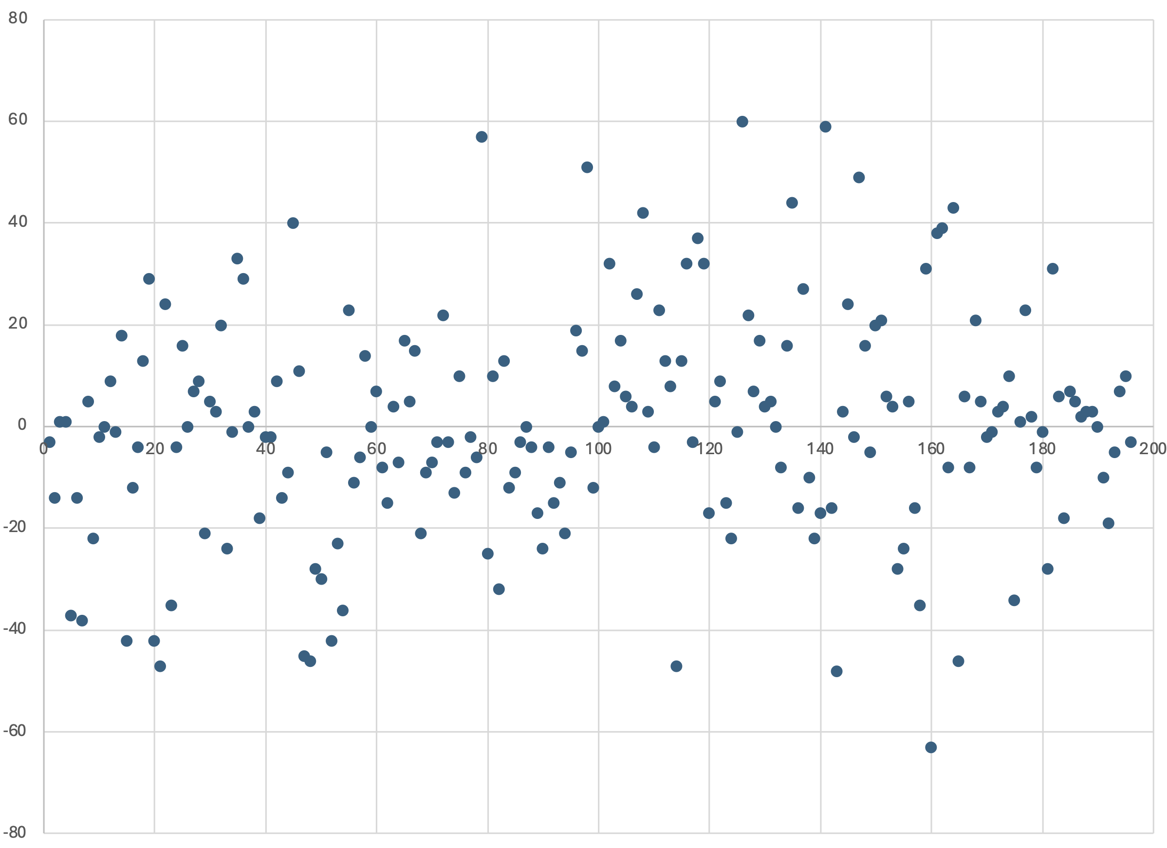
Figure 1: Scatter plot comparing the popularity of Wikidata entities (X-axis) with the prediction error (Y-axis) for the countries population feature.

Appendix B Additional Analysis

Error Analysis

Table 9 presents an error analysis for the same five rankings that were considered in Table 4. Specifically, in Table 9 we focus on the entities where the difference between the predicted ranking position and the position of the entity in the ground truth ranking is highest. On the left, we show entities which are ranked too high (i.e. where the model predicts the entity has the feature to a greater extent than is the case according to the ground truth). On the right, we show entities which are ranked too low. In the case of sweetness, we can see that the model consistently ranks cheeses to high. They are predicted to be in ranking positions 150-250, whereas the ground truth puts them at 500-590. In the case of saltiness, we can see that sweet drinks and pastries are ranked too high. For instance, cola soda is ranked in position 108 whereas the ground truth puts it at 517 (out of 590). Overall, these results suggest that the model struggles with certain food groups. For the features scary, funny and population, clear patterns are harder to detect.

Impact of Entity Popularity

The reliability of LLMs when it comes to modelling entity knowledge has been found to correlate with the popularity of the entities involved Mallen et al. (2023). To analyse this aspect, Figure 1 compares entity popularity with prediction error, for the countries population feature from the WD2 dataset. For this analysis, we have used the pairwise Llama2-13B model that was trained on the WD1-training split. We obtained a ranking of all countries using the SVM method with 20 samples. On the X-axis, the entities are ranked from the most popular to the least popular. On the Y-axis, we show the prediction error for the corresponding entity, measured as the difference between the position of the entity in the predicted ranking and its position in the ground truth ranking. Based on this analysis, no clear correlation between entity popularity and prediction error can be observed.

References

- Abdou et al. (2021) Mostafa Abdou, Artur Kulmizev, Daniel Hershcovich, Stella Frank, Ellie Pavlick, and Anders Søgaard. 2021. Can language models encode perceptual structure without grounding? a case study in color. In Proceedings of the 25th Conference on Computational Natural Language Learning, pages 109–132, Online. Association for Computational Linguistics.
- Aisbett and Gibbon (2001) Janet Aisbett and Greg Gibbon. 2001. A general formulation of conceptual spaces as a meso level representation. Artif. Intell., 133(1-2):189–232.
- Bender and Koller (2020) Emily M. Bender and Alexander Koller. 2020. Climbing towards NLU: On meaning, form, and understanding in the age of data. In Proceedings of the 58th Annual Meeting of the Association for Computational Linguistics, pages 5185–5198, Online. Association for Computational Linguistics.
- Bosselut et al. (2019) Antoine Bosselut, Hannah Rashkin, Maarten Sap, Chaitanya Malaviya, Asli Celikyilmaz, and Yejin Choi. 2019. COMET: Commonsense transformers for automatic knowledge graph construction. In Proceedings of the 57th Annual Meeting of the Association for Computational Linguistics, pages 4762–4779, Florence, Italy. Association for Computational Linguistics.
- Chatterjee et al. (2023) Usashi Chatterjee, Amit Gajbhiye, and Steven Schockaert. 2023. Cabbage sweeter than cake? analysing the potential of large language models for learning conceptual spaces. In Proceedings of the 2023 Conference on Empirical Methods in Natural Language Processing, pages 11836–11842, Singapore. Association for Computational Linguistics.
- Chen and Pu (2012) Li Chen and Pearl Pu. 2012. Critiquing-based recommenders: survey and emerging trends. User Model. User Adapt. Interact., 22(1-2):125–150.
- Cohen et al. (2023) Roi Cohen, Mor Geva, Jonathan Berant, and Amir Globerson. 2023. Crawling the internal knowledge-base of language models. In Findings of the Association for Computational Linguistics: EACL 2023, pages 1856–1869, Dubrovnik, Croatia. Association for Computational Linguistics.
- Derrac and Schockaert (2015) Joaquín Derrac and Steven Schockaert. 2015. Inducing semantic relations from conceptual spaces: A data-driven approach to plausible reasoning. Artif. Intell., 228:66–94.
- Devlin et al. (2019) Jacob Devlin, Ming-Wei Chang, Kenton Lee, and Kristina Toutanova. 2019. BERT: Pre-training of deep bidirectional transformers for language understanding. In Proceedings of the 2019 Conference of the North American Chapter of the Association for Computational Linguistics: Human Language Technologies, Volume 1 (Long and Short Papers), pages 4171–4186, Minneapolis, Minnesota. Association for Computational Linguistics.
- Gärdenfors (2000) Peter Gärdenfors. 2000. Conceptual Spaces - the Geometry of Thought. MIT Press.
- Geng et al. (2022) Shijie Geng, Shuchang Liu, Zuohui Fu, Yingqiang Ge, and Yongfeng Zhang. 2022. Recommendation as language processing (RLP): A unified pretrain, personalized prompt & predict paradigm (P5). In RecSys ’22: Sixteenth ACM Conference on Recommender Systems, Seattle, WA, USA, September 18 - 23, 2022, pages 299–315. ACM.
- Gienapp et al. (2022) Lukas Gienapp, Maik Fröbe, Matthias Hagen, and Martin Potthast. 2022. Sparse pairwise re-ranking with pre-trained transformers. In ICTIR ’22: The 2022 ACM SIGIR International Conference on the Theory of Information Retrieval, Madrid, Spain, July 11 - 12, 2022, pages 72–80. ACM.
- Gordon and Durme (2013) Jonathan Gordon and Benjamin Van Durme. 2013. Reporting bias and knowledge acquisition. In Proceedings of the 2013 workshop on Automated knowledge base construction, AKBC@CIKM 13, San Francisco, California, USA, October 27-28, 2013, pages 25–30. ACM.
- Guo et al. (2022) Qingyu Guo, Fuzhen Zhuang, Chuan Qin, Hengshu Zhu, Xing Xie, Hui Xiong, and Qing He. 2022. A survey on knowledge graph-based recommender systems. IEEE Trans. Knowl. Data Eng., 34(8):3549–3568.
- Gupta et al. (2015) Abhijeet Gupta, Gemma Boleda, Marco Baroni, and Sebastian Padó. 2015. Distributional vectors encode referential attributes. In Proceedings of the 2015 Conference on Empirical Methods in Natural Language Processing, pages 12–21, Lisbon, Portugal. Association for Computational Linguistics.
- Hao et al. (2023) Shibo Hao, Bowen Tan, Kaiwen Tang, Bin Ni, Xiyan Shao, Hengzhe Zhang, Eric Xing, and Zhiting Hu. 2023. BertNet: Harvesting knowledge graphs with arbitrary relations from pretrained language models. In Findings of the Association for Computational Linguistics: ACL 2023, pages 5000–5015, Toronto, Canada. Association for Computational Linguistics.
- Hase et al. (2024) Peter Hase, Mohit Bansal, Peter Clark, and Sarah Wiegreffe. 2024. The unreasonable effectiveness of easy training data for hard tasks. CoRR, abs/2401.06751.
- He et al. (2022) Yuan He, Jiaoyan Chen, Denvar Antonyrajah, and Ian Horrocks. 2022. Bertmap: A bert-based ontology alignment system. In Thirty-Sixth AAAI Conference on Artificial Intelligence, AAAI 2022, Thirty-Fourth Conference on Innovative Applications of Artificial Intelligence, IAAI 2022, The Twelveth Symposium on Educational Advances in Artificial Intelligence, EAAI 2022 Virtual Event, February 22 - March 1, 2022, pages 5684–5691. AAAI Press.
- Huang et al. (2022) James Y. Huang, Bangzheng Li, Jiashu Xu, and Muhao Chen. 2022. Unified semantic typing with meaningful label inference. In Proceedings of the 2022 Conference of the North American Chapter of the Association for Computational Linguistics: Human Language Technologies, pages 2642–2654, Seattle, United States. Association for Computational Linguistics.
- Kotkov et al. (2022) Denis Kotkov, Alan Medlar, Alexandr V. Maslov, Umesh Raj Satyal, Mats Neovius, and Dorota Glowacka. 2022. The tag genome dataset for books. In CHIIR ’22: ACM SIGIR Conference on Human Information Interaction and Retrieval, Regensburg, Germany, March 14 - 18, 2022, pages 353–357. ACM.
- Li et al. (2023) Lei Li, Jingjing Xu, Qingxiu Dong, Ce Zheng, Xu Sun, Lingpeng Kong, and Qi Liu. 2023. Can language models understand physical concepts? In Proceedings of the 2023 Conference on Empirical Methods in Natural Language Processing, pages 11843–11861, Singapore. Association for Computational Linguistics.
- Liu et al. (2022a) Fangyu Liu, Julian Eisenschlos, Jeremy Cole, and Nigel Collier. 2022a. Do ever larger octopi still amplify reporting biases? evidence from judgments of typical colour. In Proceedings of the 2nd Conference of the Asia-Pacific Chapter of the Association for Computational Linguistics and the 12th International Joint Conference on Natural Language Processing (Volume 2: Short Papers), pages 210–220, Online only. Association for Computational Linguistics.
- Liu et al. (2022b) Xiao Liu, Da Yin, Yansong Feng, and Dongyan Zhao. 2022b. Things not written in text: Exploring spatial commonsense from visual signals. In Proceedings of the 60th Annual Meeting of the Association for Computational Linguistics (Volume 1: Long Papers), pages 2365–2376, Dublin, Ireland. Association for Computational Linguistics.
- Mallen et al. (2023) Alex Mallen, Akari Asai, Victor Zhong, Rajarshi Das, Daniel Khashabi, and Hannaneh Hajishirzi. 2023. When not to trust language models: Investigating effectiveness of parametric and non-parametric memories. In Proceedings of the 61st Annual Meeting of the Association for Computational Linguistics (Volume 1: Long Papers), pages 9802–9822, Toronto, Canada. Association for Computational Linguistics.
- Martin et al. (2014) Christophe Martin, Michel Visalli, Christine Lange, Pascal Schlich, and Sylvie Issanchou. 2014. Creation of a food taste database using an in-home “taste” profile method. Food Quality and Preference, 36:70–80.
- Merullo et al. (2023) Jack Merullo, Louis Castricato, Carsten Eickhoff, and Ellie Pavlick. 2023. Linearly mapping from image to text space. In The Eleventh International Conference on Learning Representations, ICLR 2023, Kigali, Rwanda, May 1-5, 2023. OpenReview.net.
- Nogueira et al. (2019) Rodrigo Frassetto Nogueira, Wei Yang, Kyunghyun Cho, and Jimmy Lin. 2019. Multi-stage document ranking with BERT. CoRR, abs/1910.14424.
- Nosofsky et al. (2018) Robert M Nosofsky, Craig A Sanders, Brian J Meagher, and Bruce J Douglas. 2018. Toward the development of a feature-space representation for a complex natural category domain. Behavior Research Methods, 50:530–556.
- Paik et al. (2021) Cory Paik, Stéphane Aroca-Ouellette, Alessandro Roncone, and Katharina Kann. 2021. The World of an Octopus: How Reporting Bias Influences a Language Model’s Perception of Color. In Proceedings of the 2021 Conference on Empirical Methods in Natural Language Processing, pages 823–835, Online and Punta Cana, Dominican Republic. Association for Computational Linguistics.
- Patel and Pavlick (2022) Roma Patel and Ellie Pavlick. 2022. Mapping language models to grounded conceptual spaces. In International Conference on Learning Representations.
- Petroni et al. (2019) Fabio Petroni, Tim Rocktäschel, Sebastian Riedel, Patrick Lewis, Anton Bakhtin, Yuxiang Wu, and Alexander Miller. 2019. Language models as knowledge bases? In Proceedings of the 2019 Conference on Empirical Methods in Natural Language Processing and the 9th International Joint Conference on Natural Language Processing (EMNLP-IJCNLP), pages 2463–2473, Hong Kong, China. Association for Computational Linguistics.
- Qin et al. (2023) Zhen Qin, Rolf Jagerman, Kai Hui, Honglei Zhuang, Junru Wu, Jiaming Shen, Tianqi Liu, Jialu Liu, Donald Metzler, Xuanhui Wang, and Michael Bendersky. 2023. Large language models are effective text rankers with pairwise ranking prompting. CoRR, abs/2306.17563.
- Reinanda et al. (2020) Ridho Reinanda, Edgar Meij, and Maarten de Rijke. 2020. Knowledge graphs: An information retrieval perspective. Found. Trends Inf. Retr., 14(4):289–444.
- Roberts et al. (2020) Adam Roberts, Colin Raffel, and Noam Shazeer. 2020. How much knowledge can you pack into the parameters of a language model? In Proceedings of the 2020 Conference on Empirical Methods in Natural Language Processing (EMNLP), pages 5418–5426, Online. Association for Computational Linguistics.
- Schneider et al. (2022) Phillip Schneider, Tim Schopf, Juraj Vladika, Mikhail Galkin, Elena Simperl, and Florian Matthes. 2022. A decade of knowledge graphs in natural language processing: A survey. In Proceedings of the 2nd Conference of the Asia-Pacific Chapter of the Association for Computational Linguistics and the 12th International Joint Conference on Natural Language Processing (Volume 1: Long Papers), pages 601–614, Online only. Association for Computational Linguistics.
- Søgaard (2023) Anders Søgaard. 2023. Grounding the vector space of an octopus: Word meaning from raw text. Minds Mach., 33(1):33–54.
- Standley et al. (2017) Trevor Standley, Ozan Sener, Dawn Chen, and Silvio Savarese. 2017. image2mass: Estimating the mass of an object from its image. In 1st Annual Conference on Robot Learning, CoRL 2017, Mountain View, California, USA, November 13-15, 2017, Proceedings, volume 78 of Proceedings of Machine Learning Research, pages 324–333. PMLR.
- Sun et al. (2019) Fei Sun, Jun Liu, Jian Wu, Changhua Pei, Xiao Lin, Wenwu Ou, and Peng Jiang. 2019. Bert4rec: Sequential recommendation with bidirectional encoder representations from transformer. In Proceedings of the 28th ACM International Conference on Information and Knowledge Management, CIKM 2019, Beijing, China, November 3-7, 2019, pages 1441–1450. ACM.
- Ushio et al. (2023) Asahi Ushio, José Camacho-Collados, and Steven Schockaert. 2023. A relentless benchmark for modelling graded relations between named entities. CoRR, abs/2305.15002.
- Vig et al. (2012) Jesse Vig, Shilad Sen, and John Riedl. 2012. The tag genome: Encoding community knowledge to support novel interaction. ACM Trans. Interact. Intell. Syst., 2(3):13:1–13:44.
- Vigna (2016) Sebastiano Vigna. 2016. Spectral ranking. Network Science, 4(4):433–445.
- Wauthier et al. (2013) Fabian L. Wauthier, Michael I. Jordan, and Nebojsa Jojic. 2013. Efficient ranking from pairwise comparisons. In Proceedings of the 30th International Conference on Machine Learning, ICML 2013, Atlanta, GA, USA, 16-21 June 2013, volume 28 of JMLR Workshop and Conference Proceedings, pages 109–117. JMLR.org.
- West et al. (2022) Peter West, Chandra Bhagavatula, Jack Hessel, Jena Hwang, Liwei Jiang, Ronan Le Bras, Ximing Lu, Sean Welleck, and Yejin Choi. 2022. Symbolic knowledge distillation: from general language models to commonsense models. In Proceedings of the 2022 Conference of the North American Chapter of the Association for Computational Linguistics: Human Language Technologies, pages 4602–4625, Seattle, United States. Association for Computational Linguistics.
- Yao et al. (2019) Liang Yao, Chengsheng Mao, and Yuan Luo. 2019. KG-BERT: BERT for knowledge graph completion. CoRR, abs/1909.03193.
- Yu et al. (2023) Changlong Yu, Weiqi Wang, Xin Liu, Jiaxin Bai, Yangqiu Song, Zheng Li, Yifan Gao, Tianyu Cao, and Bing Yin. 2023. FolkScope: Intention knowledge graph construction for E-commerce commonsense discovery. In Findings of the Association for Computational Linguistics: ACL 2023, pages 1173–1191, Toronto, Canada. Association for Computational Linguistics.
- Zhu et al. (2024) Jian-Qiao Zhu, Haijiang Yan, and Thomas L. Griffiths. 2024. Recovering mental representations from large language models with markov chain monte carlo.