Iterative Inversion of (ELAA-)MIMO Channels Using Symmetric Rank-$1$ Regularization

Abstract

While iterative matrix inversion methods excel in computational efficiency, memory optimization, and support for parallel and distributed computing when managing large matrices, their limitations are also evident in multiple-input multiple-output (MIMO) fading channels. These methods encounter challenges related to slow convergence and diminished accuracy, especially in ill-conditioned scenarios, hindering their application in future MIMO networks such as extra-large aperture array (ELAA). To address these challenges, this paper proposes a novel matrix regularization method termed symmetric rank-$1$ regularization (SR-$1$R). The proposed method functions by augmenting the channel matrix with a symmetric rank-$1$ matrix, with the primary goal of minimizing the condition number of the resultant regularized matrix. This significantly improves the matrix condition, enabling fast and accurate iterative inversion of the regularized matrix. Then, the inverse of the original channel matrix is obtained by applying the Sherman-Morrison transform on the outcome of iterative inversions. Our eigenvalue analysis unveils the best channel condition that can be achieved by an optimized SR-$1$R matrix. Moreover, a power iteration-assisted (PIA) approach is proposed to find the optimum SR-$1$R matrix without need of eigenvalue decomposition. The proposed approach exhibits logarithmic algorithm-depth in parallel computing for MIMO precoding. Finally, computer simulations demonstrate that SR-$1$R has the potential to reduce iterative iterations by up to $33\%$, while also significantly improve symbol error probability by approximately an order of magnitude.

I Introduction

Iterative matrix inversion methods play a pivotal role in scenarios where direct methods become impractical or computationally expensive. This significance becomes especially pronounced when handling large matrices, as iterative techniques offer superior computational and memory efficiency, enhanced numerical stability, and support for parallel and distributed computing [2, 3, 4, 5]. These attributes distinctly position iterative methods as advantageous over direct inversion techniques. Despite their promise, current iterative methods face difficulties with slow convergence and reduced accuracy in ill-conditioned scenarios. This limitation restricts their potential application in future wireless multi-antenna (i.e., MIMO) networks, particularly evident in the case of extra-large aperture array (ELAA) (see [6, 7, 8] for the concept of ELAA). This is because ELAA-MIMO features significant channel spatial inconsistency on the network side, introducing spatial non-stationarity in the ELAA channel and exacerbating the ill-conditioning of the MIMO channel beyond what is typical in conventional MIMO systems [9, 10, 11, 12, 13, 14, 15, 16]. Notably, these challenges are not unique to iterative matrix inversion methods. Linear system inverse approaches like the Broyden-Fletcher-Goldfarb-Shanno (BFGS) algorithm and sketch-and-projection, sidestepping matrix inversion, also confront similar issues [17, 18, 19, 20].

Basically, the channel condition can be improved by means of matrix regularization, pre-conditioning or a combination of them. The regularized zero-forcing (RZF) stands as a widely used regularization method, yet our research reveals its subpar performance in iterative channel inversion (see Section V). In contrast, pre-conditioning involves multiplying a specialized matrix with the original channel matrix, often formed from a sub-matrix inverse [21, 22, 23, 24]. This approach enhances matrix conditions, leading to improved iterative inversion in numerous classical methods like Jacobi [21], Gauss-Seidel (GS) [22], and symmetric successive over-relaxation (SSOR) [23, 24]. However, simulation results elaborated in Section V unveils their inability to deliver satisfactory performance in ill-conditioned ELAA-MIMO channels.

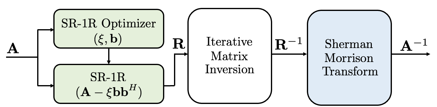
Figure 1: Block diagram of the proposed symmetric rank-$1$ regularization for iterative matrix inversion.

This paper introduces a novel channel matrix regularization approach, termed symmetric rank-$1$ regularization (SR-$1$R). As per the block diagram illustrated in Fig. 1, we consider a positive definite matrix $\mathbf{A}\in\mathbb{C}^{N\times N}$, where $N$ represents the matrix size. Rather than directly computing the inverse matrix $\mathbf{A}^{-1}$, the aim of SR-$1$R is to firstly find the inverse of a rank-$1$ regularized matrix $\mathbf{R}\in\mathbb{C}^{N\times N}$ defined as:

$$\mathbf{R}\triangleq\mathbf{A}-\xi\mathbf{b}\mathbf{b}^{H},$$ (1)

where $\xi\in\mathbb{R}$ is a scaling factor, $\mathbf{b}\in\mathbb{C}^{N\times 1}$ is a unitary vector (i.e., $\|\mathbf{b}\|=1$), $[\cdot]^{H}$ and $\|\cdot\|$ denotes the Hermitian transpose and the Euclidean norm, respectively. Next, Sherman-Morrison transform (see [25]) is applied on $\mathbf{R}^{-1}$, resulting in:

$$\mathbf{A}^{-1}=\mathbf{R}^{-1}-\frac{\xi\mathbf{R}^{-1}\mathbf{b}\mathbf{b}^{H}\mathbf{R}^{-1}}{1+\xi\mathbf{b}^{H}\mathbf{R}^{-1}\mathbf{b}}.$$ (2)

Our research aims to ascertain the existence of $(\xi,\mathbf{b})$ values that could improve the condition of $\mathbf{R}$ compared to $\mathbf{A}$. If such values exist, our goal is to optimize $(\xi,\mathbf{b})$ to maximize the channel condition.

Alongside the novel SR-$1$R concept, major contributions of our research include:

I-1 Feasibility and optimality study of SR-$1$R

Our study, through eigenvalue analysis, reveals the presence of an optimal $(\xi,\mathbf{b})$ combination that maximizes the matrix condition of $\mathbf{R}$. Detailed results and justifications are referred to Section III.

I-2 Practical approaches for optimization

While theoretically, optimal determination of $(\xi,\mathbf{b})$ involves eigenvalue decomposition (EVD) or singular value decomposition (SVD) of $\mathbf{A}$, these methods conflict with the purpose of employing iterative matrix inversion, particularly in wireless MIMO scenarios where direct matrix inversion is unfeasible.

To tackle this challenge, our research reveals that $(\xi,\mathbf{b})$ can be optimally established solely by discerning the largest and smallest eigenvalues of $\mathbf{A}$ and their corresponding eigenvectors. Subsequently, we employ a power iteration technique to compute the largest eigenvalue of $\mathbf{A}$ and a shifted power iteration method to compute the smallest eigenvalue, concurrently obtaining their respective eigenvectors. It is shown that sufficiently accurate estimates of eigenvalues and eigenvectors can be obtained through just two iterations.

I-3 Simulations and Performance Evaluation

The SR-$1$R approach has undergone extensive simulations and performance evaluation across a range of MIMO fading channel types, encompassing identical and independently distributed (i.i.d.) symmetric MIMO Rayleigh channels, i.i.d symmetric MIMO Rician channels, line-of-sight (LoS)-dominated ELAA-MIMO channels, and LoS/non-LoS mixed ELAA-MIMO channels [9]. These channels exhibit diverse and contrasting channel conditions. Our simulation results consistently demonstrate that the SR-$1$R approach substantially enhances the channel conditions in all of these channel models. Thanks to this remarkable advantage, the SR-$1$R-based iterative channel inversion exhibits a significant performance enhancement in MIMO linear precoding, leading to substantial reduction in average symbol-error-rate (SER) by an order of magnitude. Simultaneously, the number of required iterations is generally reduced by more than $4\%$. In the case of the i.i.d. MIMO Rician channel, the reduction in the number of iterations even reaches $33\%$.

The rest of this paper is organized as follows. Section II presents the system model and problem statement. Section III presents the concept of SR-$1$R and the optimality study. Section IV presents practical approaches to attain the SR-$1$R optimality. Section V presents simulation results and performance evaluation. Finally, conclusion and outlook are presented in Section VI.

II System Model, Prior Art, and Problem Analysis

The SR-$1$R approach exhibits broad applicability across various scenarios necessitating iterative matrix inversion. However, our paper specifically concentrates on its implementation within wireless MIMO channel inversion, particularly tailored to MIMO linear precoding technology. This focus is motivated by the prevalent significance of MIMO linear precoding in advanced wireless communication systems, where channel inversion holds critical role for optimizing signal transmission efficiency and reducing interference, making it an ideal area for SR-$1$R exploration.

II-A MIMO Linear Precoding

Consider MIMO downlink communications, where an access point (i.e., the transmitter) equipped with $M$ transmit-antennas sends $N$ independent data streams to $N$ $(\leq M)$ user antennas, respectively. Denote $\mathbf{s}\in\mathbb{C}^{N\times 1}$ as an information-bearing symbol block in the spatial domain. To maintain the orthogonality between data streams, an interference-rejection linear precoder (IR-LP), denoted as $\mathbf{W}\in\mathbb{C}^{M\times N}$, is employed at the transmitter, which yields the transmit symbol block:

$$\mathbf{x}=\mathbf{W}\mathbf{s}.$$ (3)

The symbol block received through the MIMO channel $(\mathbf{H}\in\mathbb{C}^{N\times M})$ is represented by:

$$\mathbf{y}=\sqrt{\mathcal{E}}\mathbf{H}\mathbf{x}+\mathbf{v},$$ (4)

where $\mathbf{y}\in\mathbb{C}^{N\times 1}$ stands for the received block, $\mathcal{E}$ for the transmit power, $\mathbf{v}\sim\mathcal{CN}(\mathbf{0},\sigma_{v}^{2}\mathbf{I}_{N})$ for the additive white Gaussian noise (AWGN), and $\mathbf{I}_{N}$ for the identity matrix with the dimension of $N$.

A commonly employed IR-LP is known as the zero-forcing (ZF) precoder [26], i.e.,

$$\mathbf{W}\triangleq\mathbf{H}^{H}\mathbf{A}^{-1},~{}\mathbf{A}\triangleq\mathbf{H}\mathbf{H}^{H}\in\mathbb{C}^{N\times N},$$ (5)

where the Gram matrix $\mathbf{A}$ is positive definite. Applying (5) into (4) yields

$$\mathbf{y}=\sqrt{\mathcal{E}}\mathbf{s}+\mathbf{v}.$$ (6)

With the ZF precoder, data streams do not interfere with each other and can be decoded separately. On the other hand, the computation of matrix inverse $\mathbf{A}^{-1}$ costs cubic complexity and does not support well the parallel computing technology [27, 28]. This presents a formidable challenge in the design of scalable large-MIMO systems.

In the realm of MIMO, it is important to note that RZF is regarded as a prominent IR-LP approach. However, in this paper, we will explore RZF as a regularization method in Sec. II-B.

II-B Prior Art Analysis

Our analysis of prior art identifies two main categories of iterative solutions to the inversion problem: a) iterative linear system inversion, and b) iterative matrix inversion. This subsection briefly explores both categories, laying the groundwork for advocating the necessity of employing iterative matrix inversion.

II-B1 Iterative linear system inversion

In numerous use cases, the matrix inverse problem can be circumvented by transforming it into a linear system inverse problem. Specifically for the linear ZF precoding problem (5), rather than directly computing $\mathbf{A}^{-1}$, we can find a vector $\overline{\mathbf{x}}\in\mathbb{C}^{N\times 1}$ that is related to $\mathbf{x}$ through the equation: $\mathbf{x}=\mathbf{H}^{H}\overline{\mathbf{x}}$. In line with (5), the goal is to iteratively solve the following equation (e.g., [19, 29, 30]):

$$\mathbf{A}\overline{\mathbf{x}}=\mathbf{s}.$$ (7)

An analogous approach can also be found in the MIMO uplink detection (e.g., [18, 11, 12]). In the context of iterative linear system inversion, two significant issues come to the forefront: 1) the performance of iterative linear system inversion is highly susceptible to the condition of the matrix $\mathbf{A}$. As shown in Section V, when dealing with ELAA-MIMO channels, which are often ill-conditioned, these iterative algorithms are too sub-optimal; 2) some inverse problems, like MIMO non-linear precoding (see [31, 32, 33, 34, 28]) cannot be transformed into the linear system inverse problems. In these cases, matrix inversion becomes a necessary step.

II-B2 Iterative matrix inversion

Various techniques are available for the iterative matrix inversion. Common methods include the Neumann series method [2] and the Schulz method [3]. The Schulz method is also known as the Hotelling-Bodewig algorithm [4] or the Newton iteration [18, 35] in the literature. Additionally, the sketch-and-projection approach has been recently adopted for matrix inversion [5]. Our state-of-the-art analysis concludes that the Neumann series method typically requires more iterations compared to the Schulz method [35]. Furthermore, the performance of the sketch-and-projection method is influenced by the randomness of the sketching process, making it less stable than the Schulz method. Therefore, in this paper, we opt for the Schulz method to evaluate the performance of iterative matrix inversion concerning the condition numbers $\kappa(\mathbf{A})$ or $\kappa(\mathbf{R})$.

Specifically, considering $\mathbf{X}_{i}$ as the output of the $i^{th}$ iteration of iterative matrix inversion, the convergence criterion for an iterative algorithm is represented by the Frobenius norm converging as:

$$\lim_{i\to\infty}\|\mathbf{I}-\mathbf{A}\mathbf{X}_{i}\|_{\mathrm{F}}=0,$$ (8)

i.e., $\mathbf{X}_{\infty}=\mathbf{A}^{-1}$. To achieve this goal, the Schulz method suggests the following iterative process:

$$\mathbf{X}_{i} =\omega\mathbf{A}^{H},~{}i=0$$

$$\mathbf{X}_{i} =2\mathbf{X}_{i-1}-\mathbf{X}_{i-1}\mathbf{A}\mathbf{X}_{i-1},~{}i>0,$$ (9)

where $\omega$ is a scaling factor ensuring the condition

$$\rho(\mathbf{I}-\omega\mathbf{A}\mathbf{A}^{H})<1,$$ (10)

and $\rho(\cdot)$ is the spectrum radius of a matrix.

II-C Research Problem and Analysis

For the iterative matrix inversion, the number of iterations should be minimized while ensuring satisfactory performance, as this is crucial for maximizing computational efficiency and accuracy. The number of iterations is strongly dependent on the condition number $\kappa(\mathbf{A})$. For instance, in the case of a unitary channel matrix with $\kappa(\mathbf{A})=1$, setting $\omega=1$ in (II-B2) immediately yields $\|\mathbf{I}-\mathbf{A}\mathbf{X}_{0}\|_{\mathrm{F}}=0$.

As far as MIMO fading channels are concerned, it is empirically evident that the number of iterations grows rapidly as the condition number $\kappa(\mathbf{A})$ increases.

This challenge is particularly pronounced in the case of ELAA-MIMO channels, which often experience poorer channel conditions compared to traditional MIMO channels due to their network-side spatial channel inconsistency. Hence, there is a pressing need to find an efficient approach to enhance the condition number of ELAA-MIMO channels

The current approaches for improving the condition of the channel matrix mainly involve matrix regularization and preconditioning techniques. A widely recognized matrix regularization method is known as the RZF, which performs the iterative inversion on the regularized matrix

$$\mathbf{R}_{\textsc{rzf}}=(\mathbf{A}+\rm{snr}^{-1}\mathbf{I}),$$ (11)

where $\rm{snr}$ denotes the signal-to-noise ratio (SNR). Our simulation results, presented in Section V, demonstrate that the RZF method generally does not provide satisfactory performance when applied to invert ELAA-MIMO channels. Notably, RZF exhibits particularly poor performance at high SNRs. This is easily understandable because, under high SNRs, $\mathbf{R}_{\textsc{rzf}}$ is almost identical to $\mathbf{A}$.

For the pre-conditioning method, the channel matrix $\mathbf{A}$ is multiplied with a pre-conditioning matrix $\mathbf{P}^{-1}$, which yields

$$\mathbf{R}_{\textsc{pre}}=\mathbf{P}^{-1}\mathbf{A}.$$ (12)

Iterative inversion is performed on $\mathbf{R}_{\textsc{pre}}$, which aims to generate

$$\mathbf{R}_{\textsc{pre}}^{-1}=\mathbf{A}^{-1}\mathbf{P}.$$ (13)

After the iterative inversion, $\mathbf{A}^{-1}$ is computed through $\mathbf{A}^{-1}=\mathbf{R}_{\textsc{pre}}^{-1}\mathbf{P}^{-1}$.

Prior art pre-conditioning methods mainly include the Jacobi pre-conditioning [21], the GS pre-conditioning [22, 19], and the SSOR pre-conditioning [24]. Their major difference lies in the formation of the pre-conditioning matrix $\mathbf{P}$, i.e.,

$$\rm{Jacobi}:\quad \mathbf{P}=\mathbf{D};$$ (14)

$$\rm{GS}:\quad \mathbf{P}=\mathbf{D}+\mathbf{L};$$ (15)

$$\rm{SSOR}:\quad \mathbf{P}=(\mathbf{D}+\mathbf{L})\mathbf{D}^{-1}(\mathbf{D}+\mathbf{L})^{H},$$ (16)

where $\mathbf{D}$ is a diagonal matrix formed by the diagonal of $\mathbf{A}$, and $\mathbf{L}$ is the strict lower triangular part of $\mathbf{A}$. It is perhaps worth noting that inverting a lower-triangular matrix entails a computational complexity that scales quadratically, which keeps both the GS and SSOR approaches within the realm of low complexity methods.

Despite extensive prior research documented in the literature, pre-conditioning approaches have only yielded marginal performance enhancements when dealing with ill-conditioned ELAA-MIMO channels (as detailed in Section V). To further enhance both the performance and convergence in iterative matrix inversion, we introduce the SR-$1$R method.

III SR-$1$R: Feasibility and Optimality Study

The concept of SR-$1$R has already been introduced in Section I, as outlined in Eqn. (1)-(2). In this section, our objective is to address the question of whether there exists $(\xi,\mathbf{b})$ that can lead to:

• $\kappa(\mathbf{R})<\kappa(\mathbf{A})$;

• minimization of $\kappa(\mathbf{R})$.

This question motivates the feasibility and optimality study, relying on the assumption of availability of EVD (or SVD as appropriate). This assumption is reasonable here as it is specifically for feasibility and optimality analysis.

As a quick overview of our finding, upon defining eigenvalues of the positive-definite matrix $\mathbf{A}$ as $(\lambda_{0},\lambda_{1},...,\lambda_{N-1})$, arranged in descent order, our mathematical analysis reveals the existence of $(\xi,\mathbf{b})$ yielding:

$$\min\big{(}\kappa(\mathbf{R})\big{)}=\frac{\lambda_{1}}{\lambda_{N-2}}.$$ (17)

This condition number is smaller than the condition number of $\mathbf{A}$

$$\kappa(\mathbf{A})=\frac{\lambda_{0}}{\lambda_{N-1}},$$ (18)

signifying a notable improvement. Further elaboration and detailed proof of this finding are provided in the subsequent subsections.

III-A Feasibility Study

Similar to $\mathbf{A}$, Eqn. (1) shows that $\mathbf{R}$ is also a symmetric matrix. However, $\mathbf{R}$ may not exhibit positive-definite properties, introducing a degree of complexity into the mathematical analysis of its condition number.

To facilitate our analysis, we express the regularized matrix $\mathbf{R}$ as the following form

$$\mathbf{R}=\mathbf{U}(\mathbf{\Lambda}-\xi\mathbf{p}\mathbf{p}^{H})\mathbf{U}^{H},$$ (19)

where $\mathbf{\Lambda}\triangleq\rm{diag}\{\lambda_{0},\lambda_{1},...,\lambda_{N-1}\}$, $\mathbf{U}\in\mathbb{C}^{N\times N}$ is the unitary matrix coming from the EVD: $\mathbf{A}=\mathbf{U\Lambda U}^{H}$, and $\mathbf{p}\triangleq\mathbf{U}^{H}\mathbf{b}$.

Consider the matrix $\mathbf{\Theta}$ defined as

$$\mathbf{\Theta}\triangleq\mathbf{\Lambda}-\xi\mathbf{p}\mathbf{p}^{H}.$$ (20)

It is worthwhile to note that $\mathbf{\Theta}$ and $\mathbf{R}$ possess identical eigenvalues, and consequently have $\kappa(\mathbf{\Theta})=\kappa(\mathbf{R})$. Hence, our investigation can be directed towards the analysis of $\mathbf{\Theta}$.

In the mathematical literature, (20) is well known as the rank-$1$ modification of symmetric eigenproblem [36, 37]. One of the significant findings from previous research can be summarized as:

Lemma 1 (from [37])

Define the eigenvalues of the rank-$1$ modified symmetric matrix $\mathbf{\Theta}$ as $(\theta_{0},\theta_{1},...,\theta_{N-1})$. When $\xi<0$, $\mathbf{\Theta}$ is a positive-definite matrix whose eigenvalues satisfies the following inequalities

$$\lambda_{0}\leq\theta_{0}\leq\lambda_{0}-\xi,$$

$$\lambda_{n}\leq\theta_{n}\leq\lambda_{n-1},~{}_{n=1,\cdots,N-1}.$$ (21)

When $\xi>0$, the following inequalities are satisfied

$$\lambda_{N-1}-\xi\leq\theta_{N-1}\leq\lambda_{N-1},$$

$$\lambda_{n+1}\leq\theta_{n}\leq\lambda_{n},~{}_{n=0,\cdots,N-2}.$$ (22)

According to Lemma 1, when $\xi<0$, the matrix $\mathbf{\Theta}$ is positive-definite, and its eigenvalues coincide with its singular values. The condition number of $\mathbf{\Theta}$ can be determined using (1), expressed as

$$\kappa(\mathbf{\Theta})=\frac{\theta_{0}}{\theta_{N-1}}\in\left[\frac{\lambda_{0}}{\lambda_{N-2}},\frac{\lambda_{0}-\xi}{\lambda_{N-1}}\right].$$ (23)

However, in this case, it cannot be guaranteed that the inequality $\kappa(\mathbf{\Theta})<\kappa(\mathbf{A})$ holds. Consequently, having $\xi<0$ is not conducive for the SR-$1$R approach.

For the case of $\xi>0$, $\mathbf{\Theta}$ is not necessarily a positive-definite matrix, and thus its eigenvalues do not coincide with its singular values. As per (1), the only inconsistency comes from $\theta_{N-1}$, which can be either positive or negative ($\xi\neq\lambda_{N-1}$). Therefore, the smallest singular value of $\mathbf{\Theta}$, denoted as $\overline{\theta}_{\min}$, is

$$\overline{\theta}_{\min}=\min(|\theta_{N-1}|,\theta_{N-2}),$$ (24)

and the largest singular value of $\mathbf{\Theta}$, denoted as $\overline{\theta}_{\max}$, is

$$\overline{\theta}_{\max}=\max(|\theta_{N-1}|,\theta_{0}),$$ (25)

where $|\cdot|$ stands for the absolute value of a number. Then, the condition number of $\mathbf{\Theta}$ can be expressed as

$$\kappa(\mathbf{\Theta})=\frac{\overline{\theta}_{\max}}{\overline{\theta}_{\min}}=\frac{\max(|\theta_{N-1}|,\theta_{0})}{\min(|\theta_{N-1}|,\theta_{N-2})}.$$ (26)

To analyze (26) more thoroughly, we must rely on the following result:

Theorem 1

When $\mathbf{\Theta}$ is neither positive-definite nor positive semi-definite, there exists a $\xi(>0)$ such that the smallest eigenvalue of $\mathbf{\Theta}$ (i.e., $\theta_{N-1}$) satisfies

$$-\theta_{0}<\theta_{N-1}<-\theta_{N-2}.$$ (27)

Proof:

We prove a sufficient condition of Theorem 1: $\theta_{N-1}$ monotonically decreases from $0$ to $-\infty$ as $\xi$ increases from $\xi^{\bot}$ to $\infty$, where $\xi^{\bot}$ is a positive scalar explained later in (31).

To facilitate our study, define $f(\theta,\xi)$ as

$$f(\theta,\xi)\triangleq\det(\mathbf{\Theta}-\theta\mathbf{I})=\det(\mathbf{\Lambda}-\xi\mathbf{p}\mathbf{p}^{H}-\theta\mathbf{I}),$$ (28)

where $\det(\cdot)$ stands for the determinant of a matrix. $\theta_{N-1}$ is the smallest root of $f(\theta,\xi)=0$.

After some tedious mathematical work, the closed form expression of $f(\theta,\xi)$ is given by

$$f(\theta,\xi) =(-\theta)^{N}$$

$$+ \sum_{n=0}^{N-1}(-\theta)^{N-1-n}\Big{(}e_{n+1}(\mathbf{\Lambda})-\xi\sum_{k=0}^{N-1}e_{n}(\overline{\mathbf{\Lambda}}_{k})|p_{k}|^{2}\Big{)},~{}~{}~{}~{}$$ (29)

where $e_{n+1}(\mathbf{\Lambda})$ stands for the $(n+1)^{th}$ order elementary symmetric function (ESF) formed by $\lambda_{0},\cdots,\lambda_{N-1}$ and $e_{n}(\overline{\mathbf{\Lambda}}_{k})$ for the $n^{th}$ order ESF formed by $\lambda_{0},\cdots,\lambda_{k-1},\lambda_{k+1},\cdots,\lambda_{N-1}$ [38]. Since $\lambda_{n}>0$ $\forall n$, we have $e_{n+1}(\mathbf{\Lambda})>0$ and $e_{n}(\overline{\mathbf{\Lambda}}_{k})>0$ $\forall n,k$.

The proof is divided into three steps. In the first step, we prove

$$\theta_{N-1}<0~{}\mathrm{for}~{}\xi>\xi^{\bot},$$ (30)

where $\xi^{\bot}$ is given by

$$\xi^{\bot}=\frac{e_{N}(\mathbf{\Lambda})}{\sum_{k=0}^{N-1}e_{N-1}(\overline{\mathbf{\Lambda}}_{k})|p_{k}|^{2}}.$$ (31)

Substituting (31) into (III-A) when $\theta=0$ yields $f(0,\xi)=e_{N}(\mathbf{\Lambda})(1-\xi/\xi^{\bot})$. Thus, we have

$$f(0,\xi)<0~{}\mathrm{for}~{}\xi>\xi^{\bot}.$$ (32)

When $\theta\to-\infty$, $f(\theta,\xi)$ is dominated by the term with the highest order:

$$\lim\limits_{\theta\to-\infty}f(\theta,\xi)=\lim\limits_{\theta\to-\infty}(-\theta)^{N}=\infty.$$ (33)

Since $\theta_{N-1}$ is the only root within $(-\infty,\lambda_{N-1})$, it must fall into $(-\infty,0)$ for $\xi>\xi^{\bot}$ according to the intermediate value theorem. (30) is proved.

In the second step, we prove that $\theta_{N-1}$ monotonically decreases with the increase of $\xi$ when $\xi>\xi^{\bot}$, i.e.,

$$\theta_{N-1}^{(2)}<\theta_{N-1}^{(1)}<0~{}\mathrm{for}~{}\xi^{(2)}>\xi^{(1)}>\xi^{\bot}.$$ (34)

This monotonicity can be proved by studying the following partial derivative:

$$\frac{\partial f(\theta,\xi)}{\partial\xi}=\sum_{n=0}^{N-1}(-\theta)^{N-1-n}\Big{(}-\sum_{k=0}^{N-1}e_{n}(\overline{\mathbf{\Lambda}}_{k})|p_{k}|^{2}\Big{)}.$$ (35)

When $\theta<0$, (35) is negative. Since $\theta_{N-1}^{(1)}<0$, the following inequality holds

$$f(\theta_{N-1}^{(1)},\xi^{(2)})<f(\theta_{N-1}^{(1)},\xi^{(1)})=0.$$ (36)

(36) indicates $\theta_{N-1}^{(2)}\in(-\infty,\theta_{N-1}^{(1)})$ according to the intermediate value theorem, and proves (34).

The first two steps prove that $\theta_{N-1}(<0)$ monotonically decreases with the increase of $\xi(>\xi^{\bot})$. In the final step, we prove that

$$\lim\limits_{\xi\to\infty}\theta_{N-1}=-\infty.$$ (37)

Since $\|\mathbf{p}\|=1$, we have

$$\sum_{n=0}^{N-1}\theta_{n}=\mathrm{Tr}(\mathbf{\Theta})=\mathrm{Tr}(\mathbf{\Lambda}-\xi\mathbf{p}\mathbf{p}^{H})=\sum_{n=0}^{N-1}\lambda_{n}-\xi.$$ (38)

The right hand side of (38) tends to $-\infty$ as $\xi\to\infty$. Recall (1) that $\theta_{n,}$ _n=0,⋯,N-2 is bounded. Hence, we must have $\theta_{N-1}\to-\infty$ as $\xi\to\infty$ in the left hand side. (37) is proved.

Therefore, $\theta_{N-1}$ monotonically decreases from $0$ to $-\infty$ as $\xi$ increases from $\xi^{\bot}$ to $\infty$, yielding Theorem 1. ∎

The result (27) immediately leads to the inequality

$$\theta_{0}>|\theta_{N-1}|>\theta_{N-2}.$$ (39)

Applying (39) and (1) into (26) yields

$$\kappa(\mathbf{R})=\kappa(\mathbf{\Theta})<\frac{\theta_{0}}{\theta_{N-2}}\leq\frac{\lambda_{0}}{\lambda_{N-1}}=\kappa(\mathbf{A}).$$ (40)

This intermediate result ensures the feasibility of employing SR-$1$R to improve the matrix condition. Nevertheless, an in-depth study is needed to establish the optimality of SR-$1$R.

III-B Optimality Study

In addition to the upper bound in (40), as per (1), it is evident that $\theta_{0}\geq\lambda_{1}$ and $\theta_{N-2}\leq\lambda_{N-2}$, and (26) yields also the following lower bound

$$\kappa(\mathbf{\Theta})\geq\frac{\lambda_{1}}{\lambda_{N-2}}.$$ (41)

This result indicates the best matrix condition that can be possibly achieved via the SR-$1$R approach.

From a mathematical perspective, determining the optimal configuration of $(\xi,\mathbf{p})$ in a general form is extremely challenging. Nevertheless, we have successfully identified a special case of $(\xi,\mathbf{p})$ that is optimum, achieving the lower bound specified in (41).

In this specific case, the vector $\mathbf{p}$ are configured as:

$$\mathbf{p}=[\alpha,0,...,0,\beta]^{T},\alpha,\beta\neq 0,\alpha^{2}+\beta^{2}=1.$$ (42)

Applying (42) into (20) results in

$$\mathbf{\Theta}=\left[\begin{array}[]{ccccc}\lambda_{0}-\xi\alpha^{2}&0&\cdots&0&-\xi\alpha\beta\\ 0&\lambda_{1}&0&\cdots&0\\ \vdots&\vdots&\ddots&\vdots&\vdots\\ 0&0&\cdots&\lambda_{N-2}&0\\ -\xi\alpha\beta&0&\cdots&0&\lambda_{N-1}-\xi\beta^{2}\end{array}\right]$$ (43)

Immediately, we can identify $(\lambda_{1},\lambda_{2},...,\lambda_{N-2})$ as eigenvalues of $\mathbf{\Theta}$. The remaining two eigenvalues stem from a sub-matrix of $\mathbf{\Theta}$, constituted by:

$$\overline{\mathbf{\Theta}}=\left[\begin{array}[]{cc}\lambda_{0}-\xi\alpha^{2}&-\xi\alpha\beta\\ -\xi\alpha\beta&\lambda_{N-1}-\xi\beta^{2}\end{array}\right],$$ (44)

and satisfy the equation

$$\det(\overline{\mathbf{\Theta}}-\theta\mathbf{I})=0.$$ (45)

The quadratic form of (45) is expressed by

$$\theta^{2}-(\lambda_{0}+\lambda_{N-1}-\xi)\theta$$

$$\quad\quad\quad\quad+\lambda_{0}\lambda_{N-1}-\xi(\alpha^{2}\lambda_{N-1}+\beta^{2}\lambda_{0})=0.$$ (46)

Re-arranging (III-B) as the following form

$$\xi=\frac{(\theta-\lambda_{0})(\theta-\lambda_{N-1})}{\alpha^{2}\lambda_{N-1}+\beta^{2}\lambda_{0}-\theta}.$$ (47)

To achieve the lower bound in (41), we expect one eigenvalue (i.e., $\theta_{0}$) to meet the condition

$$\theta_{0}=\lambda_{1},$$ (48)

while the other (i.e., $\theta_{N-1}$) fulfills the condition

$$|\theta_{N-1}|\geq\lambda_{N-1},$$ (49)

$$|\theta_{N-1}|\leq\lambda_{1}.$$ (50)

Meeting the condition in (49) is relatively straightforward. Therefore, our primary focus in this study will revolve around satisfying conditions (48) and (50).

Applying (48) into (47) yields

$$\xi=\frac{(\lambda_{1}-\lambda_{0})(\lambda_{1}-\lambda_{N-1})}{\alpha^{2}\lambda_{N-1}+\beta^{2}\lambda_{0}-\lambda_{1}}.$$ (51)

Furthermore, the condition (49) is equivalent to: $\theta_{N-1}\leq-\lambda_{N-2}$. It is trivial to justify that $\xi$ is a monotonically decreasing function of $\theta$ within the range of $\theta\in(-\infty,0)$. Therefore, a sufficient condition to satisfy (49) is

$$\xi \geq\frac{(\lambda_{N-2}+\lambda_{0})(\lambda_{N-2}+\lambda_{N-1})}{\alpha^{2}\lambda_{N-1}+\beta^{2}\lambda_{0}+\lambda_{N-2}}$$ (52)

$$>\frac{(\lambda_{N-2}+\lambda_{0})(\lambda_{N-2}+\lambda_{N-1})}{\alpha^{2}\lambda_{0}+\beta^{2}\lambda_{0}+\lambda_{N-2}}$$ (53)

$$>\lambda_{N-2}+\lambda_{N-1}$$ (54)

where the inequality (53) holds due to: $\lambda_{0}>\lambda_{N-1}$.

Substituting (51) into (54) yields

$$\frac{(\lambda_{1}-\lambda_{0})(\lambda_{1}-\lambda_{N-1})}{\alpha^{2}\lambda_{N-1}+\beta^{2}\lambda_{0}-\lambda_{1}}>\lambda_{N-2}+\lambda_{N-1}>0.$$ (55)

Due to $(\lambda_{1}-\lambda_{0})<0$ and $(\lambda_{1}-\lambda_{N-1})>0$, the configuration of $(\alpha,\beta)$ must adhere to:

$$\alpha^{2}\lambda_{N-1}+\beta^{2}\lambda_{0}-\lambda_{1}<0.$$ (56)

Considering (56), solving (55) yields:

$$\beta^{2}>\left(\frac{\lambda_{1}-\lambda_{N-1}}{\lambda_{0}-\lambda_{N-1}}\right)\left(\frac{\lambda_{1}-\lambda_{0}}{\lambda_{N-2}+\lambda_{N-1}}+1\right).$$ (57)

Given that the expression on the right-hand side of (57) is surely smaller than $1$, it is always possible to find a value for $\beta$ that satisfies this inequality. Finally, the feasibility analysis can be concluded as:

Theorem 2

To achieve the lower bound specified in (41), it suffices to simultaneously satisfy the inequalities (54) and (57) for $(\xi,\beta)$.

After determining the value of $\beta$, the vector ($\mathbf{p}$) can be constructed using (42), following which $\mathbf{b}$ is formed as:

$$\mathbf{b}=\mathbf{U}\mathbf{p}.$$ (58)

IV Power Iteration-Assisted Approach for The Implementation of SR-$1$R

The theoretical framework presented in Section III relies on the availability of EVD. As already discussed in Section I, assuming the availability of EVD contradicts the objective of employing iterative matrix inversion. This motivates us to propose a power iteration-assisted (PIA) approach, which can determine $(\xi,\mathbf{b})$ without need of EVD.

IV-A The Proposed PIA Approach

The PIA approach builds upon the principles of Theorem 2, incorporating certain relaxations and approximations. Our key conclusion is stated in the following theorem.

Theorem 3

Consider an ill-conditioned matrix $\mathbf{A}$ with its eigenvalues satisfying $\lambda_{0}\gg\lambda_{N-2}$ and $\lambda_{1}\gg\lambda_{N-2}$. A sufficient condition for $\kappa(\mathbf{\Theta})$ to achieve the lower bound specified in (41) is:

$$\xi=\lambda_{0};$$ (59)

$$\frac{\lambda_{N-2}}{\lambda_{0}}\ll\beta<\frac{\lambda_{1}}{\lambda_{0}}.$$ (60)

Proof:

Theorem 2 indicates that $\xi$ should fulfill the condition (54). Given $\lambda_{0}\gg\lambda_{N-2}$ and $\lambda_{N-2}>\lambda_{N-1}$, setting $\xi$ as specified in (59) is sufficient to guarantee the fulfillment of condition (54). Then, we plug (59) into (III-B) and obtain

$$x^{2}-\lambda_{N-1}x+\beta^{2}\lambda_{0}\lambda_{N-1}-\beta^{2}\lambda_{0}^{2}=0,$$ (61)

where the notation $x$ is utilized in place of $\theta$ to prevent potential confusion.

Solving (61) gives two roots, corresponding to two eigenvalues of $\mathbf{\Theta}$:

$$x_{1}=\frac{1}{2}\left(\lambda_{N-1}+\sqrt{\lambda_{N-1}^{2}+\Delta^{2}}\right),$$ (62)

$$x_{2}=\frac{1}{2}\left(\lambda_{N-1}-\sqrt{\lambda_{N-1}^{2}+\Delta^{2}}\right),$$ (63)

where $\Delta$ is expressed as:

$$\Delta^{2}=4\beta^{2}\lambda_{0}(\lambda_{0}-\lambda_{N-1}).$$ (64)

From (62) and (63), it is straightforward to see: $|x_{2}|<x_{1}$. Given the condition (60), $\lambda_{N-1}$ in (62)-(64) is negligibly small and thus omitted. Then, (62) and (63) can be approximately written as:

$$x_{1}\approx\beta\lambda_{0},~{}x_{2}\approx-\beta\lambda_{0}.$$ (65)

Applying (60) into (65), the following relationship is evident

$$\lambda_{N-2}\ll|x_{2}|<x_{1}<\lambda_{1}.$$ (66)

In this case, $\lambda_{1}$ and $\lambda_{N-2}$ become the maximum and minimum singular values of $\mathbf{\Theta}$, respectively. This immediately leads to the conclusion: $\kappa(\mathbf{R})=\kappa(\mathbf{\Theta})=\lambda_{1}/\lambda_{N-2}$. Theorem 3 is therefore proved. ∎

Theorem 3 is appealing mainly for two reasons: 1) $\xi$ becomes exclusively reliant on $\lambda_{0}$. Given that $\lambda_{0}$ stands as the largest eigenvalue of $\mathbf{A}$, it can be readily acquired using the power iteration algorithm specified in Algorithm 2, eliminating the necessity for EVD computations; 2) the condition (60) offers sufficient flexibility in determining $\beta$. For instance, $\beta$ can be specified as follows:

$$\beta \triangleq\frac{\mathrm{trace}(\mathbf{A})-\lambda_{0}}{(N-1)\lambda_{0}}$$ (67)

$$=\frac{\frac{1}{N-1}\sum_{n=1}^{N-1}\lambda_{n}}{\lambda_{0}}.$$ (68)

The numerator of (68) is the average over eigenvalues $(\lambda_{1},\lambda_{2},...,\lambda_{N-1})$. It is trivial to justify that $\beta$ satisfies the condition (66). Notably, $\beta$ defined in this form only requires the estimation of $\lambda_{0}$.

The last step is to form $\mathbf{b}$. Applying (42) into (58) results in

$$\mathbf{b}=\alpha\mathbf{u}_{0}+\beta\mathbf{u}_{N-1},~{}\alpha^{2}+\beta^{2}=1,$$ (69)

where $\mathbf{u}_{0}$, $\mathbf{u}_{N-1}$ are the $0^{th}$ and $(N-1)^{th}$ column of $\mathbf{U}$, respectively. Since $\mathbf{u}_{0}$ is the eigenvector corresponding to the largest eigenvalue $\lambda_{0}$, it can also be determined through the power iteration algorithm.

Determining $\mathbf{u}_{N-1}$, the eigenvector corresponding to the smallest eigenvalue $\lambda_{N-1}$, poses some difficulty. The most commonly used algorithm is known as the inverse power iteration [39], which applies power iteration on $\mathbf{A}^{-1}$ as $\mathbf{u}_{N-1}$ corresponds to the largest eigenvalue of $\mathbf{A}^{-1}$. However, our primary objective revolves around computing $\mathbf{A}^{-1}$, making its assumed availability impractical.

The other commonly used method is referred to the shifted power iteration, which applies the power iteration algorithm on

$$\mathbf{\Phi}=\mathbf{A}+\gamma\mathbf{I}.$$ (70)

The key is to find a suitable parameter $\gamma$ such that $\mathbf{u}_{0}$ corresponds to the maximum eigenvalue of $\mathbf{\Phi}$. In this paper, we redefine the shifted power iteration as

$$\mathbf{\Phi}=\gamma\mathbf{I}-\mathbf{A},$$ (71)

and specify $\gamma$ as

$$\gamma=\mathrm{trace}(\mathbf{A}).$$ (72)

By this means, eigenvalues of $\mathbf{\Phi}$ are expressed as

$$\phi_{n}=\sum_{k=0}^{N-1}\lambda_{k},~{}k\neq N-1-n.$$ (73)

The largest eigenvalue of $\mathbf{\Phi}$ is $\phi_{N-1}$, which is corresponding to the eigenvector $\mathbf{u}_{N-1}$. Then, applying the power iteration algorithm (Algorithm 2) on $\mathbf{\Phi}$ yields the estimate of $\mathbf{u}_{N-1}$.

Finally, the proposed PIA approach for SR-$1$R implementation is summarized in Algorithm 1.

Algorithm 1 Pseudo code of the PIA for the SR-$1$R

0:  Positive-definite Hermitian matrix $\mathbf{A}$;

0:  $\mathbf{A}^{-1}$;

1:  Feed $\mathbf{A}$ into the power iteration function (Algorithm 2) to acquire the estimate of $\lambda_{0}$ (denoted as $\hat{\lambda}_{0}$) and the estimate of $\mathbf{u}_{0}$ (denoted as $\hat{\mathbf{u}}_{0}$);

2:  Compute $\xi$ and $\beta$ using (59) and (67), respectively.

3:  Construct the matrix $\mathbf{\Phi}$ in form of (71);

4:  Feed $\mathbf{\Phi}$ into Algorithm 2 to acquire the estimate of $\mathbf{u}_{N-1}$ (denoted as $\hat{\mathbf{u}}_{N-1}$);

5:  Compute the vector $\mathbf{b}$ via (69);

6:  Form the matrix $\mathbf{R}$ via (1) and compute $\mathbf{R}^{-1}$ through the Schulz method specified in (II-B2);

7:  Compute $\mathbf{A}^{-1}$ via the Sherman-Morrison transform (2);

8:  return  $\mathbf{A}^{-1}$.

IV-B Convergence of The PIA Approach

The PIA approach heavily depends on employing the power iteration algorithm to derive essential parameters including $\lambda_{0}$, $\mathbf{u}_{0}$, and $\mathbf{u}_{N-1}$. Introducing pseudo code that demonstrates the power iteration algorithm could offer valuable insights to readers interested in understanding our performance analysis. To this end, we provide the power iteration algorithm in (Algorithm 2), where the matrix $\mathbf{A}$ is employed as a showcase. Nevertheless, $\mathbf{A}$ can be easily replaced by any Gram matrix such as $\mathbf{\Phi}$.

Algorithm 2 Pseudo code of the power iteration algorithm

0:  Matrix ($\mathbf{A}$), Tolerance ($\eta$);

0:  The largest eigenvalue ($\lambda_{0}$), the eigenvector $\mathbf{u}_{0}$;

1:  Initialize a random vector $\mathbf{u}$ and $\lambda_{\textsc{old}}=\|\mathbf{u}\|$;

2:  Normalize $\mathbf{u}$: $\mathbf{u}=\mathbf{u}/\|\mathbf{u}\|$;

3:  Compute $\mathbf{v}=\mathbf{A}\mathbf{u}$;

4:  Compute $\lambda=\|\mathbf{v}\|$;

5:  Let $\mathbf{u}=\mathbf{v}/\|\mathbf{v}\|$;

6:  If $|\lambda-\lambda_{\textsc{old}}|<\eta$ then break;

7:  Let $\lambda_{\textsc{old}}=\lambda$ and goto step $3$;

8:  return  $\lambda_{0}=\lambda$, $\mathbf{u}_{0}=\mathbf{u}$.

The convergence behavior of the power iteration algorithm has been studied in the literature [40] as:

$$\lambda\rightarrow\lambda_{0}+\underbrace{\sum_{n=1}^{N-1}\left(\frac{\lambda_{n}}{\lambda_{0}}\right)^{i}c_{n}}_{\triangleq\widetilde{\lambda}(i)},$$ (74)

where $i$ is the number of power iterations, and $c_{n},\forall n,$ are coefficients related to both eigenvectors of $\mathbf{A}$ and the initial vector $\mathbf{u}$. For ill-conditioned systems where $\lambda_{0}$ is dominating (e.g., $\lambda_{0}\gg\lambda_{1}$), the term $\widetilde{\lambda}(i)$ in (74) becomes negligibly small only after a couple of iterations. This is mostly the case for ELAA-MIMO systems.

However, for the matrix $\mathbf{\Phi}$ specified in (71), the convergence behavior becomes

$$\phi\rightarrow\phi_{0}+\underbrace{\sum_{n=1}^{N-1}\left(\frac{\phi_{n}}{\phi_{0}}\right)^{i}c^{\prime}_{n}}_{\triangleq\widetilde{\lambda}(i)},$$ (75)

where $c_{n}^{\prime},\forall n,$ are corresponding coefficients. When the values of $c_{n}^{\prime},\forall n,$ exhibit comparability among themselves, the dominant factor influencing convergence is expressed by

$$\frac{\phi_{1}}{\phi_{0}}=\frac{\lambda_{N-1}+\sum_{k=0}^{N-3}\lambda_{k}}{\lambda_{N-2}+\sum_{k=0}^{N-3}\lambda_{k}}.$$ (76)

Given that the eigenvalues $(\lambda_{N-1},\lambda_{N-2})$ are significantly smaller compared to the sum of the remaining eigenvalues, the ratio specified in (76) is close to $1$. Consequently, this leads to notably slow convergence when determining the eigenvector $\mathbf{u}_{N-1}$. In order to speed up the convergence, an enhanced PIA approach is proposed in Section IV-C.

IV-C Enhanced PIA Approach

The opportunity for convergence acceleration arises from the coefficients $c_{n}^{\prime},\forall n$, in (75). Following the principle of power iteration [40], the coefficients $c_{n}^{\prime},\forall n,$ are related to the matrix $\mathbf{\Phi}$ and the initial vector $\mathbf{u}$. Given that $\mathbf{\Phi}$ and $\mathbf{u}$ are randomly generated and independent of each other, $\mathbf{c}^{\prime}\triangleq(c_{1}^{\prime},c_{2}^{\prime},...,c_{N-1}^{\prime})^{T}$ can be viewed as a randomly generated sequence normalized in the sequence norm.

Define $\mbox{\boldmath$\mathcal{\phi}$}(i)\triangleq(\phi_{1}^{i},\phi_{2}^{i},...,\phi_{N-1}^{i})^{T}/\phi_{0}^{i}$ and represent the term $\widetilde{\lambda}(i)$ in (75) as the following vector form

$$\widetilde{\lambda}(i)=\mbox{\boldmath$\mathcal{\phi}$}^{T}(i)\mathbf{c}^{\prime}.$$ (77)

Given the matrix $\mathbf{\Phi}$, $\mathbf{c}^{\prime}$ is solely dependent on $\mathbf{u}$. When producing $L$ independent generations of $\mathbf{u}$ denoted as $\mathbf{u}_{0},\mathbf{u}_{1},...,\mathbf{u}_{L-1}$, their corresponding vectors $\mathbf{c}_{0}^{\prime},\mathbf{c}_{1}^{\prime},...,\mathbf{c}_{L-1}^{\prime}$ are generated. Then, the enhanced PIA (e-PIA) approach aims at solving the following objective function

$$l^{\star}=\underset{l}{\arg\min}|\mbox{\boldmath$\mathcal{\phi}$}^{T}(i)\mathbf{c}^{\prime}_{l}|,~{}_{l=0,...,L-1}.$$ (78)

This optimization problem can be easily managed via the power iteration algorithm specified in Algorithm 2. For various generations of $\mathbf{u}$ (or equivalently $\mathbf{c}^{\prime}$), the power iteration algorithm can run in parallel. The power iteration process related to $l^{\star}$ will be the first to reach the saturation point $\eta$ as specified in Step 6 of Algorithm 2, and consequently have the convergence accelerated.

Generally, it is mathematically challenging to quantify the gain of convergence acceleration. However, we can find a faster convergence speed that can be achieved when $\mathbf{c}^{\prime}\triangleq(0,0,...,1)^{T}$. In this extreme case, the dominating factor influencing convergence becomes

$$\frac{\phi_{N-1}}{\phi_{0}}=\frac{\lambda_{N-1}+\sum_{k=1}^{N-2}\lambda_{k}}{\lambda_{0}+\sum_{k=1}^{N-2}\lambda_{k}}.$$ (79)

For ill-conditioned systems where $\lambda_{0}$ is the dominant eigenvalue, this factor is significantly smaller than the one outlined in (76).

IV-D Scalability Analysis for SR-$1$R

In this subsection, we analyze the scalability of the SR-$1$R in comparison to the preconditioning techniques, considering both the overall complexity and the algorithm-depth. The algorithm-depth describes the minimum computing steps when employing parallel computing and determines the shortest processing time [41]. We are interested in this measurement as the compatibility to parallel computing is an important benefit of the iterative matrix inversion [1]. We will demonstrate that the PIA and e-PIA also have good parallel computing compatibility.

Before discussing Algorithm 1, we present some basic conclusions of the algorithm-depth when the computing units are assumed sufficient: The multiplication of a matrix/vector by a $N\times 1$ vector yields a depth of $\mathcal{O}(\log_{2}N)$; the summation of $N$ scalars yields a depth of $\mathcal{O}(\log_{2}N)$ (e.g., calculating the trace of a $N\times N$ matrix or the norm of a $N\times 1$ vector) [41].

Then, we analyze the PIA approach (Algorithm 1) step by step.

• Step $1$. Each iteration of Algorithm 2 calculates a matrix-vector multiplication and a norm of a vector, yielding an algorithm-depth of $\mathcal{O}(2\log_{2}N)$. Denote the iteration number to calculate $\hat{\mathbf{u}}_{0}$ by $\tau_{0}$, the total algorithm-depth is $\mathcal{O}(2\tau_{0}\log_{2}N)$. The corresponding complexity is $\mathcal{O}(\tau_{0}(N^{2}+N))$.

• Step $2$. $\xi$ is the direct output of Algorithm 2 in Step $1$. The calculation of $\beta$ requires $\mathrm{Tr}(\mathbf{A})$. This has $\mathcal{O}(\log_{2}N)$ algorithm-depth and $\mathcal{O}(N)$ complexity.

• Step $3$. With $\mathrm{Tr}(\mathbf{A})$ already available in Step $2$, the calculation of $\mathbf{\Phi}$ has $\mathcal{O}(N)$ complexity and negligible depth.

• Step $4$. Denote the iteration number to compute $\hat{\mathbf{u}}_{N-1}$ by $\tau_{N-1}$. The algorithm-depth is $\mathcal{O}(2\tau_{N-1}\log_{2}N)$ and the complexity is $\mathcal{O}(\tau_{N-1}(N^{2}+N))$.

• Step $5$. The summation of two vectors has $\mathcal{O}(N)$ complexity and negligible depth.

• Step $6$. This step belongs to the iterative matrix inversion, and does not count into the regularization. A good regularization/preconditioning technique accelerates this process. This will be discussed in detail in Section V-C Experiment 4.

• Step $7$. The second term of the Sherman-Morrison transform (recall (2)) can be decomposed into three matrix-vector multiplications and a vector-vector outer product. Note the matrix-vector multiplications can be computed in parallel, and the outer product has negligible depth. This yields an algorithm-depth of $\mathcal{O}(\log_{2}N)$. The deduction between the first and second terms has $\mathcal{O}(N^{2})$ complexity and negligible depth. Hence, this step has $\mathcal{O}(\log_{2}N)$ algorithm-depth and $\mathcal{O}(5N^{2})$ complexity in total.

Aggregating the analysis yields an overall complexity of Algorithm 1:

$$\mathcal{O}((\tau_{0}+\tau_{N-1}+5)N^{2}+3N).$$ (80)

Step $1\sim 2$ and Step $3\sim 4$ can be computed in parallel. Hence, the total algorithm-depth is dependent on the maximal iteration number of Step $1\&4$ as given by

$$\tau_{\max}\triangleq\max(\tau_{0},\tau_{N-1}).$$ (81)

Then, the overall algorithm-depth of Algorithm 1 is

$$\mathcal{O}((2\tau_{\max}+2)\log_{2}N).$$ (82)

When employing the e-PIA, additional complexity is introduced and upper bounded by $\mathcal{O}((L-1)\tau_{\max}(N^{2}+N))$. But the algorithm-depth remains the same because different candidates are computed in parallel.

In comparison, the GS and SSOR preconditioning require the inversion of a triangular matrix, i.e., a complexity of $\mathcal{O}(N^{2})$ [11]. This is usually done by the Gauss-Jordan elimination, and constitutes $N$ iterations [42]. Hence, the algorithm-depth is $\mathcal{O}(N)$. Table I compares the algorithm-depths numerically w.r.t. the size $N$ when $\tau_{\max}=1$ (as in Section V), where the PIA/e-PIA approaches show significant advantages to the GS and SSOR when $N>16$.

TABLE I: Comparison of algorithm-depth with baselines

	PIA/e-PIA	GS	SSOR
$N$	$\mathcal{O}((2\tau_{\max}+2)\log_{2}N)$	$\mathcal{O}(N)$	$\mathcal{O}(N)$
$N=16$	$16$	$16$	$16$
$N=64$	$24$	$64$	$64$
$N=128$	$28$	$128$	$128$

V Simulation Results and Discussion

In this section, computer simulations are carried out to demonstrate the performance of both the PIA and e-PIA approaches for the SR-$1$R. As an overview, the results are divided into four experiments (see Section V-C):

• Experiment 1 investigates the condition number improvement of the PIA approach.

• Experiment 2 investigates the improvement of the e-PIA compared to the PIA approach.

• Experiment 3 compares the RZF to the ZF when using iterative linear precoding.

• Experiment 4 compares both the PIA and e-PIA against the baselines in terms of the iteration number and average SER of the iterative linear precoding.

V-A Implementation of the SR-$1$R

Setting the convergence threshold $\eta$ in Algorithm 2 could be difficult in implementation. This is because the $\eta$ could be reached due to bad initialization. The increment of Algorithm 2 is given by

$$\lambda-\lambda_{\textsc{old}}=\sum_{n=1}^{N-1}\Big{(}\frac{\lambda_{n}}{\lambda_{0}}\Big{)}^{i-1}\Big{(}\frac{\lambda_{n}}{\lambda_{0}}-1\Big{)}.$$ (83)

(83) means the increment approaches zero in two cases: when $i\to\infty$, or when $(\lambda_{n})/(\lambda_{0})\approx 1$. When $\mathbf{u}$ is badly initialized, i.e., $\lambda_{n}\approx\lambda_{0}$, it is hard to determine the convergence. This brings troubles to the PIA and e-PIA approaches to calculate $\hat{\mathbf{u}}_{N-1}$ .

To handle this problem, we fix the iteration number of Algorithm 2 in the implementation, i.e., $\tau_{0}=\tau_{N-1}=\tau$. Moreover, to avoid picking the wrong candidate in the e-PIA, each candidate is fed into the iterative matrix inversion to produce an inversion result, denoted by $\mathbf{A}^{-1}_{l}$, _l=0,⋯,L-1. Then, we choose the inversion result that minimizes the residual error as the output of the e-PIA approach:

$$\mathbf{A}^{-1}=\operatorname*{arg\,min}_{\mathbf{A}^{-1}_{l}}\|\mathbf{I}-\mathbf{A}\mathbf{A}^{-1}_{l}\|^{2}_{\mathrm{F}}.$$ (84)

Notably, the algorithm-depth of the e-PIA approach remains logarithmic with this implementation. The computation of each candidate can be parallelized. The calculation of the residual error is a summation of $N^{2}$ scalars, and has an algorithm-depth of $\mathcal{O}(2\log_{2}N)$. The ordering of the residual error has a depth of $\mathcal{O}(\log_{2}L)$ [41]. Therefore, the simulation implementation does not fundamentally change the algorithm-depth in Tab I.

In the implementation of the SR-$1$R, we need to ensure the Schulz method is always convergent. Recall (10) and replace $\mathbf{A}$ with $\mathbf{R}$, we need $\rho(\mathbf{I}-\omega\mathbf{R}\mathbf{R}^{H})<1$. To this end, the Gershgorin circle theorem (see [24]) is employed:

$$\omega_{\mathrm{Ger}}=\big{(}\max_{n}(\sum_{i=0}^{N-1}|\mathbf{R}_{n}^{H}\mathbf{R}_{i}|)\big{)}^{-1},$$ (85)

where $\mathbf{R}_{n}$ stands for the $n^{th}$ column of $\mathbf{R}$.

V-B Baselines and Simulation Setup

We consider three types of baselines for the studies of the SR-$1$R, as shown in Table II. The iterative matrix inversion alone and the preconditioning are included to show the improvement of the SR-$1$R on the condition number (see Experiment 1$\sim$3). In the study of iterative linear precoding, the linear system inverse is also included since it serves the same purpose as iterative matrix inversion (see Experiment 4). Both the BFGS algorithm and the sketch-and-projection have demonstrated remarkable reliability advantage in the recent studies [19, 18, 17, 20].

TABLE II: Simulation Baselines

Iterative Matrix Inversion	Schulz Method [3]
Preconditioning	Jacobi [21]
	GS [22]
	SSOR [23, 24]
Linear System Inverse	BFGS Algorithm [29]
	Sketch-and-Projection [19, 18]

We consider two types of ELAA channel and two types of stationary ill-conditioned channel in the simulation. The channel model in [9] is adopted for the ELAA channel in appreciation of its comprehensive consideration of mixed LoS/non-LoS states, shadowing effects and path-loss. In ELAA systems, we consider the height of users and the base station to be $1.5$ m and $10$ m, respectively.

• LoS-dominated ELAA: The ill condition arises from the correlation of the LoS paths. We consider $M=64$, $N=16$ (single user), and the vertical distance from the user to the ELAA is $40$ m.

• Symmetric Mixed LoS/non-LoS ELAA: The ill condition arises from both the correlation of the LoS paths and the symmetric MIMO size. The MIMO size is configured as : $M=N=128$ ($8$ users with $16$ antennas each), and the vertical distance from users to the ELAA is $40$ m. The users are equally spaced along a parallel line to the base station antenna array with a maximal inter-user distance of $10$ m.

• Symmetric i.i.d. Rayleigh: This type of channel has been widely considered in wireless communication studies. The ill condition arises from the symmetric MIMO size.

• Symmetric i.i.d. Rician: The ill condition arises not only from the symmetric MIMO size but also from the strong LoS correlation.

In the simulation, the wireless channel is normalized ($\|\mathbf{H}\|_{\mathrm{F}}^{2}=N$) to remove the effect of path loss in ELAA channels. The carrier frequency is $3.5$ GHz; the modulation scheme is $256$ QAM; the power iteration number is $\tau=1$.

V-C Simulation Results and Discussion

Experiment 1

This experiment aims to investigate the optimality of the PIA approach for the SR-$1$R compared to the discussion in Section III. Here we consider the ZF precoding, i.e., $\mathbf{A}=\mathbf{H}\mathbf{H}^{H}$. The performance using the RZF will be shown in Experiment 3$\sim$4.

The first thing of interest is the behavior of $\theta_{N-1}$: Theorem 1 expects $\theta_{N-1}\in(-\theta_{0},-\theta_{N-2})$. Since $\theta_{0}$ and $\theta_{N-2}$ change in each realization of the channel, we use the following measurement:

$$\frac{\theta_{N-1}-(-\theta_{N-2})}{(-\theta_{0})-(-\theta_{N-2})}=\frac{\theta_{N-1}+\theta_{N-2}}{-\theta_{0}+\theta_{N-2}}.$$ (86)

(86) falls in $(0,1)$ when $\theta_{N-1}\in(-\theta_{0},-\theta_{N-2})$.

Fig. 2 demonstrates the PDF of (86), where the solid lines stand for the ELAA channels and the dash lines for the stationary channels. It is shown that $\theta_{N-1}$ almost always falls in the expected interval. Only in the LoS-dominated ELAA, $\theta_{N-1}$ slightly exceeds the interval in the left tail for less than $5\%$. Therefore, we can say that the PIA approach successfully fulfills Theorem 1, such that $\kappa(\mathbf{R})=(\theta_{0})/(\theta_{N-2})$.

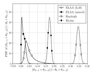
Figure 2: PDF of $(\theta_{N-1}+\theta_{N-2})/(-\theta_{0}+\theta_{N-2})$ for the PIA approach in both ELAA channels and stationary channels.

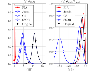
Figure 3: PDF of $(\theta_{0})/(\lambda_{1})$ and $(\theta_{N-2})/(\lambda_{N-2})$ for the e-PIA approach in LoS-dominated ELAA when $M=64$, $N=16$.

Then, we investigate the behavior of $\theta_{0}$ and $\theta_{N-2}$ compared to the optimal performance in Section III-B, i.e., $\theta_{0}=\lambda_{1}$ and $\theta_{N-2}=\lambda_{N-2}$. To this end, we examine the PDF of $(\theta_{0})/(\lambda_{1})$ and $(\theta_{N-2})/(\lambda_{N-2})$ in each wireless channel. In comparison, the behavior of the preconditioning baselines are also demonstrated. Denote the singular values of the preconditioned matrix (i.e., $\mathbf{P}^{-1}\mathbf{A}$) by $\zeta_{n}$, where $\zeta_{0}>\cdots>\zeta_{N-1}$. We have $\kappa(\mathbf{P}^{-1}\mathbf{A})=(\zeta_{0})/(\zeta_{N-1})$. By comparing $(\zeta_{0})/(\lambda_{1})$ to $(\theta_{0})/(\lambda_{1})$ and $(\zeta_{N-1})/(\lambda_{N-2})$ to $(\theta_{N-2})/(\lambda_{N-2})$, we show the difference between the PIA approach and the preconditioning.

As shown in Fig. 3$\sim$6, the black lines named ’Original’ stand for $(\lambda_{0})/(\lambda_{1})$ or $(\lambda_{N-1})/(\lambda_{N-2})$ of $\mathbf{A}$; the red circle-marked lines stand for the PIA approach; the blue lines stand for the preconditioning baselines.

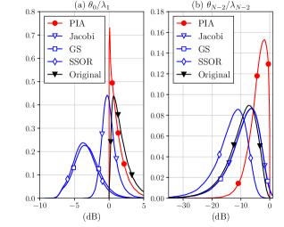
Figure 4: PDF of $(\theta_{0})/(\lambda_{1})$ and $(\theta_{N-2})/(\lambda_{N-2})$ for the e-PIA approach in symmetric mixed LoS/non-LoS ELAA when $M=N=128$.

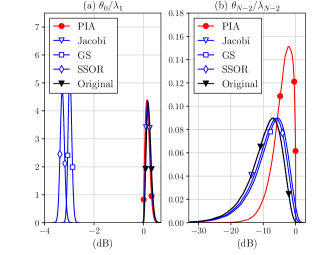
Figure 5: PDF of $(\theta_{0})/(\lambda_{1})$ and $(\theta_{N-2})/(\lambda_{N-2})$ for the e-PIA approach in symmetric i.i.d. Rayleigh channel when $M=N=128$.

Firstly, we discuss $\theta_{0}$. In LoS-dominated ELAA (Fig. 3) and symmetric i.i.d. Rician channel (Fig. 6), we have $\lambda_{0}\gg\lambda_{1}$. In these two cases, $(\theta_{0})/(\lambda_{1})$ is around $1$ dB, while $(\lambda_{0})/(\lambda_{1})$ is usually more than $10$ dB. In comparison, the preconditioning baselines have $(\zeta_{0})/(\lambda_{1})$ around $5$ dB or $10$ dB. This means the PIA approach achieves significant advantage compared to the preconditioning.

In the symmetric mixed LoS/non-LoS ELAA (Fig. 4) and symmetric i.i.d. Rayleigh channel (Fig. 5), $\lambda_{0}$ is not so dominant to $\lambda_{1}$. This limits the possible improvement of the PIA approach. In these two cases, the preconditioning baselines outperforms the PIA approach for around $3\sim 5$ dB, because $\zeta_{0}$ is not bounded by $\lambda_{1}$. Nevertheless, the PIA approach offsets this drawback when we consider $\theta_{N-2}$ later.

Secondly, we discuss $\theta_{N-2}$. In the symmetric mixed LoS/non-LoS ELAA (Fig. 4), the symmetric i.i.d. Rayleigh channel (Fig. 5) and the symmetric i.i.d. Rician channel (Fig. 6), we have $(\lambda_{N-1})/(\lambda_{N-2})$ around $-10$ dB with a left tail lower than $-30$ dB. This is due to the symmetric MIMO size. In these three cases, the PIA approach brings significant improvement: $(\theta_{N-2})/(\lambda_{N-2})$ is around $-3$ dB with a left tail of $-20$ dB. $\theta_{N-2}$ is not so close to $\lambda_{N-2}$ like $\theta_{0}$ to $\lambda_{1}$. This is because $\hat{\mathbf{u}}_{N-1}$ is not well estimated, as expected in Section IV-B. In comparison, the preconditioning baselines hardly brings any improvement. In Fig. 4 and 6, $\zeta_{N-1}$ could be even smaller than $\lambda_{N-1}$ and make the condition number more ill.

In the LoS-dominated ELAA (Fig. 3), we have $\lambda_{N-1}$ close to $\lambda_{N-2}$. In this case, $(\theta_{N-2})/(\lambda_{N-2})$ is slightly better than $(\lambda_{N-1})/(\lambda_{N-2})$. In comparison, the preconditioning baselines make $\zeta_{N-1}$ smaller than $\lambda_{N-1}$.

Overall, the PIA approach has successfully made $\theta_{0}$ close to $\lambda_{1}$, but $\theta_{N-2}$ is not so closed to $\lambda_{N-2}$. This motivates the investigation in Experiment 2.

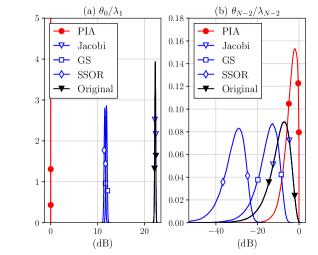
Figure 6: PDF of $(\theta_{0})/(\lambda_{1})$ and $(\theta_{N-2})/(\lambda_{N-2})$ for the e-PIA approach in symmetric i.i.d. Rician channel when $M=N=128$, K-factor$=5$.

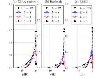
Figure 7: PDF of $(\theta_{N-1})/(\lambda_{N-2})$ of the e-PIA approach w.r.t. the list size $L$ when $M=N=128$ in (a) mixed LoS/non-LoS ELAA ($i=46$); (b) i.i.d. Rayleigh channel ($i=34$); (c) i.i.d. Rician channel ($i=34$).

Experiment 2

This experiment aims to investigate the improvement of the e-PIA approach on $\theta_{N-2}$. Fig. 7 demonstrates the PDF of $(\theta_{N-1})/(\lambda_{N-2})$ w.r.t. the list size $L$ in three cases: the mixed LoS/non-LoS ELAA, i.i.d. Rayleigh fading, and i.i.d. Rician fading. The black dash lines stand for two baselines: using the PIA approach ($L=1$), or using the e-PIA approach with the maximal list size ($L=128$). The blue and red solid lines stand for the e-PIA approach when $L=4$ or $8$, respectively.

It is shown that the e-PIA approach increases the PDF tail of $(\theta_{N-1})/(\lambda_{N-2})$ from more than $-15$ dB to around $-8$ dB. Moreover, the e-PIA approach achieves close performance to using the maximal list size when $L=4$ or $8$. This means the algorithm-depth increased by the e-PIA is not considerable.

Overall, the e-PIA demonstrates significant improvement with a reasonable list size. Later in Experiment 3 and 4, the list size of the e-PIA approach is set as $L=8$.

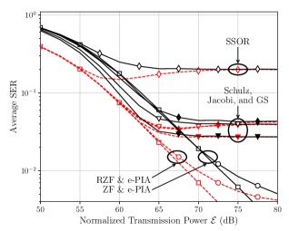
Figure 8: Average SER of the e-PIA ($i=46$), the Schulz method ($i=50$) and the preconditioning baselines ($i=50$) for the RZF and ZF w.r.t. the normalized transmission power $\mathcal{E}$ when $M=N=128$ in mixed LoS/non-LoS ELAA.

Experiment 3

This experiment aims to investigate the behavior of iterative linear precoding with the RZF compared to the ZF. It is expected that the improvement of the RZF on $\kappa(\mathbf{A})$ decreases as the SNR increases, because the regularization term is inversely proportional to the SNR (recall (11)). One may suggest fixing the regularization term of the RZF, but this deprives the RZF of its optimality as a linear precoder.

As shown in Fig. 7, the red dash lines and the black solid lines stand for the case of RZF and ZF, respectively. The RZF improves the average SER of iterative linear precoding for around $4$ dB when $\mathcal{E}=50$ dB, but gradually converges to the ZF performance. This coincides with our expectation.

In addition, two interesting phenomenons are observed. The first is that the preconditioning baselines for ZF sometimes outperforms the exact ZF precoding. This is because of the estimation error of $\mathbf{A}^{-1}$, and this error plays a similar role to the regularization term of the RZF. In contrary, the e-PIA estimates $\mathbf{A}^{-1}$ more accurately, and coincides with the exact ZF precoding when $\mathcal{E}\leq 70$ dB. The second is that the iterative linear precoding for RZF may sometimes outperform its error floor, e.g., the SSOR when $\mathcal{E}=57.5$ dB. The is because of a trade-off here: $\kappa(\mathbf{A})$ is better when $\mathcal{E}$ is smaller, but the SNR is higher when $\mathcal{E}$ is larger. The trade-off yields an optimal SER when $\mathcal{E}$ is moderate. Nevertheless, this optimal SER is close to the error floor, and does not fundamentally change the performance.

Overall, the RZF improves the SER, but does not change our major concern: the error floor of iterative linear precoding. In Experiment 4, the RZF will be employed, and the error floor of the PIA/e-PIA approaches will be compared to the baselines.

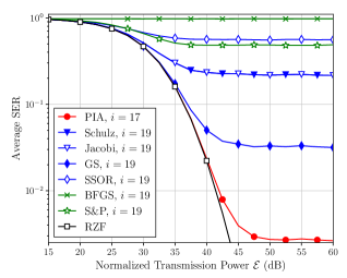
Figure 9: Average SER of the PIA/e-PIA approaches for SR-$1$R in LoS-dominated ELAA when $M=64$, $N=16$.

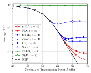
Figure 10: Average SER of the PIA/e-PIA approaches for SR-$1$R in symmetric mixed LoS/non-LoS ELAA when $M=N=128$.

Experiment 4

This experiment aims to investigate the performance of iterative linear precoding using the PIA/e-PIA approaches in terms of iteration number of iterative matrix inversion and average SER. As shown in Fig. 9$\sim$12, the red lines stand for the PIA/e-PIA approaches, the black lines for the exact RZF precoding, the blue lines for the preconditioning baselines, and the green lines for the linear system inverse baselines. The ’S&P’ stands for sketch-and-projection. Since the PIA approach almost achieves the optimal performance of SR-$1$R in the LoS-domianted ELAA (see Fig. 3), the e-PIA approach is not included in Fig. 9.

We first discuss the iteration number (recall $i$ in (II-B2)) of iterative matrix inversion. Compared to the baselines, the PIA approach reduces the iteration number for $4.0\%\sim 25.5\%$, and the e-PIA approach extends this improvement to $8.0\%\sim 33.3\%$. Hence, both the PIA/e-PIA approaches significantly improves the iteration number, and the e-PIA approach shows reasonable improvement compared to the PIA approach.

Then, we evaluate the reliability of iterative linear precoding using the SER in uncoded MIMO systems. When the SER is around $10^{-2}$, the difference of the PIA approach is less than $4$ dB from the exact RZF precoding. The e-PIA approach reduces this difference to less than $2$ dB. In comparison, all baselines fail to reach the SER of $10^{-2}$. Therefore, the PIA/e-PIA approach significantly improves the reliability of the iterative linear precoding in addition to the reduction of iteration number.

In Fig. 10 and 12, the Schulz method alone achieves the best SER among the baselines. This coincides with our observation in Fig. 4 and 6. It shows the preconditioning does not always improve the performance of iterative linear precoding.

In general, the linear system inverse achieves worse performance than the preconditioning. This is because the Schulz method converges in a local-quadratic speed, while the linear system inverse usually converges in a linear speed [5]. Hence, the Schulz method converges faster particularly when the estimation error of the precoded signal becomes stricter, e.g., when the modulation order is higher ($256$ QAM here).

Overall, both the PIA/e-PIA approaches significantly improves the iteration number of iterative matrix inversion and reliability of iterative linear precoding, and the e-PIA approach has reasonable improvement compared to the PIA approach.

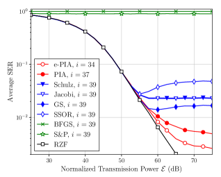
Figure 11: Average SER of the PIA/e-PIA approaches for SR-$1$R in symmetric i.i.d. Rayleigh channel when $M=N=128$.

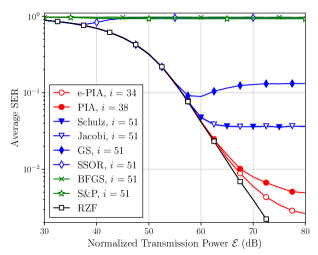
Figure 12: Average SER of the PIA/e-PIA approaches for SR-$1$R in symmetric i.i.d. Rician channel when $M=N=128$, K-factor$=5$.

VI Conclusion

In this paper, we have proposed to regularize the condition number of the channel’s Gram matrix with a symmetric rank-$1$ matrix in (ELAA)-MIMO systems, termed the SR-$1$R. The SR-$1$R can align the largest/smallest eigenvalues to their closest neighbor when the rank-$1$ matrix is formed by their corresponding eigenvectors. To enable the SR-$1$R in real-time signal processing, we have proposed the PIA approach, where the power iteration is employed to estimate these eigenvectors. Moreover, the e-PIA approach has been proposed to enhance the estimation of the eigenvector for the smallest eigenvalue. Both the PIA/e-PIA approaches have good compatibility to parallel computing with logarithmic algorithm-depth.

Simulation results have demonstrated that the PIA approach significantly improves the iteration number of iterative linear precoding for $4\%\sim 25.5\%$ in ELAA channels and stationary channels compared to the preconditioning techniques and linear system inverse; and the e-PIA approach extends the improvement to $8\%\sim 33.3\%$ Moreover, both the PIA/e-PIA approaches substantially improves the average SER for almost an order of magnitude.

References

- [1] J. Wang, Y. Ma, N. Yi, and R. Tafazolli, “Sherman-Morrison regularization for ELAA iterative linear precoding,” in Proc. IEEE Int. Conf. Commun. (ICC), 2023, pp. 3546–3552.
- [2] B. Nagy, M. Elsabrouty, and S. Elramly, “Fast converging weighted Neumann series precoding for massive MIMO systems,” IEEE Wireless Commun. Lett., vol. 7, no. 2, pp. 154–157, Apr. 2018.
- [3] G. Schulz, “Iterative berechung der reziproken matrix,” J. Appl. Math. Mech., vol. 13, no. 1, pp. 57–59, Feb. 1933.
- [4] H. Hotelling, “Some new methods in matrix calculation,” Ann. Math. Statist., vol. 14, no. 1, pp. 1–34, Mar. 1943.
- [5] R. M. Gower, “Sketch and project: Randomized iterative methods for linear systems and inverting matrices,” Ph.D. dissertation, School Math., Univ. Edinburgh, Edinburgh, U.K., 2016.
- [6] E. Björnson, L. Sanguinetti, H. Wymeersch, J. Hoydis, and T. L. Marzetta, “Massive MIMO is a reality–What is next? Five promising research directions for antenna arrays,” Digit. Signal Process., vol. 94, pp. 3–20, Nov. 2019.
- [7] M. Cui, Z. Wu, Y. Lu, X. Wei, and L. Dai, “Near-field MIMO communications for 6G: Fundamentals, challenges, potentials, and future directions,” IEEE Commun. Mag., vol. 61, no. 1, pp. 40–46, Jan. 2023.
- [8] Z. Wu and L. Dai, “Multiple access for near-field communications: SDMA or LDMA?” IEEE J. Sel. Areas Commun., vol. 41, no. 6, pp. 1918–1935, June 2023.
- [9] J. Liu, Y. Ma, and R. Tafazolli, “A spatially non-stationary fading channel model for simulation and (semi-) analytical study of ELAA-MIMO,” IEEE Trans. Wireless Commun., pp. 1–1, Oct. 2023, Early Access.
- [10] J. Liu, Y. Ma, and R. Tafazolli, “Leveraging user-wise SVD for accelerated convergence in iterative ELAA-MIMO detections,” 2023, IEEE Int. Workshop Signal Process. Advances Wireless Commun. (SPAWC).
- [11] J. Liu, Y. Ma, and R. Tafazolli, “Alternative normalized-preconditioning for scalable iterative large-MIMO detection,” 2023, IEEE Global Commun. Conf. (GLOBECOM).
- [12] J. Liu, Y. Ma, and R. Tafazolli, “Achieving maximum-likelihood detection performance with square-order complexity in large quasi-symmetric MIMO systems,” in Proc. IEEE Int. Symp. Inf. Theory (ISIT), 2023.
- [13] J. Wang, Y. Ma, N. Yi, R. Tafazolli, and F. Wang, “Network-ELAA beamforming and coverage analysis for eMBB/URLLC in spatially non-stationary Rician channels,” in Proc. IEEE Int. Conf. Commun. (ICC), 2022, pp. 3508–3513.
- [14] X. Wu, J. Sun, X. Jia, and S. Wang, “Source localization for extremely large-scale antenna arrays with spatial non-stationarity,” in Proc. IEEE Int. Conf. Acoust. Speech Signal Process. (ICASSP), 2023, pp. 1–5.
- [15] E. de Carvalho, A. Ali, A. Amiri, M. Angjelichinoski, and R. W. Heath, “Non-stationarities in extra-large-scale massive MIMO,” IEEE Wireless Commun., vol. 27, no. 4, pp. 74–80, Aug. 2020.
- [16] J. Liu, Y. Ma, J. Wang, N. Yi, R. Tafazolli, S. Xue, and F. Wang, “A non-stationary channel model with correlated NLoS/LoS states for ELAA-mMIMO,” in Proc. IEEE Global Commun. Conf. (GLOBECOM), 2021, pp. 1–6.
- [17] L. Li and J. Hu, “Fast-converging and low-complexity linear massive MIMO detection with L-BFGS method,” IEEE Trans. Veh. Technol., vol. 71, no. 10, pp. 10 656–10 665, Oct. 2022.
- [18] Z. Wang, R. M. Gower, Y. Xia, L. He, and Y. Huang, “Randomized iterative methods for low-complexity large-scale MIMO detection,” IEEE Trans. Signal Process., vol. 70, pp. 2934–2949, June 2022.
- [19] Z. Wang, J. Wang, Z. Gao, Y. Huang, D. W. K. Ng, and L. Hanzo, “Rapidly converging low-complexity iterative transmit precoders for massive MIMO downlink,” IEEE Trans. Commun., pp. 1–1, Aug. 2023.
- [20] Y. Yu, S. Zhang, J. Ying, and P. Wang, “Massive MIMO detection method based on quasi-Newton methods and deep learning,” IEEE Commun. Lett., pp. 1–1, Feb. 2024, Early Access.
- [21] J. Minango and C. de Almeida, “A low-complexity linear precoding algorithm based on Jacobi method for massive MIMO systems,” in Proc. IEEE Veh. Technol. Conf. (VTC-Spring), 2018, pp. 1–5.
- [22] W. Lee, J. Jang, J. Ro, J. Kim, and H. Song, “An efficient modified Gauss Seidel precoder for downlink massive MIMO systems,” IEEE Access, vol. 8, pp. 202 164–202 173, 2020.
- [23] T. Xie, L. Dai, X. Gao, X. Dai, and Y. Zhao, “Low-complexity SSOR-based precoding for massive MIMO systems,” IEEE Commun. Lett., vol. 20, no. 4, pp. 744–747, Apr. 2016.
- [24] Y. Saad, Iterative methods for sparse linear systems, 2nd ed. Society for Industrial and Applied Mathematics, 2003.
- [25] K. B. Petersen and M. S. Pedersen, “The matrix cookbook,” Nov. 2012.
- [26] M. Joham, W. Utschick, and J. A. Nossek, “Linear transmit processing in MIMO communications systems,” IEEE Trans. Signal Process., vol. 53, no. 8, pp. 2700–2712, July 2005.
- [27] A. Kammoun, A. Müller, E. Björnson, and M. Debbah, “Linear precoding based on polynomial expansion: Large-scale multi-cell MIMO systems,” IEEE J. Sel. Top. Signal Process., vol. 8, no. 5, pp. 861–875, Oct. 2014.
- [28] S. Yang and L. Hanzo, “Fifty years of MIMO detection: The road to large-scale MIMOs,” IEEE Commun. Surveys Tuts., vol. 17, no. 4, pp. 1941–1988, Sept. 2015.
- [29] D. Goldfarb, “Modification methods for inverting matrices and solving systems of linear algebraic equations,” Math. Comput., vol. 26, no. 120, pp. 829–852, Oct. 1972.
- [30] L. F. Richardson, “The approximate arithmetical solution by finite differences of physical problems involving differential equations, with an application to the stresses in a masonry dam,” Philos. Trans. Roy. Soc. London. Ser. A, Containing Papers Math. Physical Character, vol. 210, no. 459-470, pp. 307–357, Jan. 1911.
- [31] A. Li, Y. Ma, and R. Tafazolli, “Correlation matching pursuit for MIMO vector perturbation,” 2023, IEEE Global Commun. Conf. (GLOBECOM).
- [32] J. Wang, Y. Ma, N. Yi, R. Tafazolli, and F. Tong, “Constellation-oriented perturbation for scalable-complexity MIMO nonlinear precoding,” in Proc. IEEE Global Commun. Conf. (GLOBECOM), 2022, pp. 2413–2418.
- [33] Y. Ma, A. Yamani, N. Yi, and R. Tafazolli, “Low-complexity MU-MIMO nonlinear precoding using degree-2 sparse vector perturbation,” IEEE J. Sel. Areas Commun., vol. 34, no. 3, pp. 497–509, Feb. 2016.
- [34] B. Hochwald, C. Peel, and A. Swindlehurst, “A vector-perturbation technique for near-capacity multiantenna multiuser communication-Part II: Perturbation,” IEEE Trans. Commun., vol. 53, no. 3, pp. 537–544, Apr. 2005.
- [35] C. Tang, C. Liu, L. Yuan, and Z. Xing, “High precision low complexity matrix inversion based on Newton iteration for data detection in the massive MIMO,” IEEE Commun. Lett., vol. 20, no. 3, pp. 490–493, Mar. 2016.
- [36] G. H. Golub, “Some modified matrix eigenvalue problems,” SIAM Rev., vol. 15, no. 2, pp. 318–334, Apr. 1973.
- [37] M. Gu and S. C. Eisenstat, “A stable and efficient algorithm for the rank-one modification of the symmetric eigenproblem,” SIAM J. Matrix Anal. Appl., vol. 15, no. 4, pp. 1266–1276, Oct. 1994.
- [38] I. Macdonald, Symmetric functions and hall polynomials, 2nd ed. Clarendon Press, 1998.
- [39] R. Arablouei, K. Doğançay, and S. Werner, “Recursive total least-squares algorithm based on inverse power method and dichotomous coordinate-descent iterations,” IEEE Trans. Signal Process., vol. 63, no. 8, pp. 1941–1949, Apr. 2015.
- [40] J. Park, J. Choi, N. Lee, W. Shin, and H. V. Poor, “Rate-splitting multiple access for downlink MIMO: A generalized power iteration approach,” IEEE Trans. Wireless Commun., vol. 22, no. 3, pp. 1588–1603, Mar. 2023.
- [41] A. Grama, A. Gupta, G. Karypis, and V. Kumar, Introduction to Parallel Computing, 2nd ed. Addison-Wesley Publishing Company, 2003.
- [42] J. B. Fraleigh and R. A. Beauregard, Linear algebra, 3rd ed. Addison-Wesley Publishing Company, 1995.