Understanding Oversmoothing in Diffusion-Based GNNs
From the Perspective of Operator Semigroup Theory

Abstract

This paper presents a novel study of the oversmoothing issue in diffusion-based Graph Neural Networks (GNNs). Diverging from extant approaches grounded in random walk analysis or particle systems, we approach this problem through operator semigroup theory. This theoretical framework allows us to rigorously prove that oversmoothing is intrinsically linked to the ergodicity of the diffusion operator. This finding further poses a general and mild ergodicity-breaking condition, encompassing the various specific solutions previously offered, thereby presenting a more universal and theoretically grounded approach to mitigating oversmoothing in diffusion-based GNNs. Additionally, we offer a probabilistic interpretation of our theory, forging a link with prior works and broadening the theoretical horizon. Our experimental results reveal that this ergodicity-breaking term effectively mitigates oversmoothing measured by Dirichlet energy, and simultaneously enhances performance in node classification tasks.

1 Introduction

Graph Neural Networks (GNNs) have emerged as a powerful tool for learning graph-structured data, finding applications in various domains such as materials science (Merchant et al., 2023; Hestroffer et al., 2023), bioinformatics (Zhang et al., 2023b; Gao et al., 2023b; Strokach et al., 2020), and recommendation systems (Zhang et al., 2023a; Gao et al., 2023a). In recent years, continuous GNNs (Xhonneux et al., 2020) are proposed to generalize previous graph neural networks with discrete dynamics to the continuous domain by Neural ODE (Chen et al., 2018). Graph Diffusion Chamberlain et al. (2021b); Song et al. (2022); Choi et al. (2023) further extended the message-passing mechanism in classic GNNs under a partial differential equation (PDE) perspective. These works have made significant progress in terms of interpretability, stability, heterogeneous graphs, and beyond.

Despite these advances, a fundamental challenge of GNNs lies in the phenomenon of oversmoothing (Oono & Suzuki, 2020), where repetitions of message passing may cause node representations to become indistinguishable and thus lose their discriminative power. For GNNs with discrete dynamics, several works (Xu et al., 2018; Zhao & Akoglu, 2020; Chen et al., 2020; Rusch et al., 2023) are proposed to relieve the oversmoothing issues. Additionally, recent works (Rusch et al., 2022; Thorpe et al., 2022; Wang et al., 2023) have verified the existence of oversmoothing in GNNs with continuous dynamics and most of them address this issue by introducing additional terms in graph diffusion equations, such as source term (Thorpe et al., 2022), Allen-Cahn term (Wang et al., 2023), and reaction term (Choi et al., 2023). However, such extra terms to graph diffusion are often under specific physical scenarios without a generic and unified overview, resulting in case-specific solutions with narrow applicability.

In this paper, we propose a unified framework using operator semigroup theory to address this limitation. By viewing node features as solutions to the Cauchy problem associated with linear graph diffusion, we provide an in-depth understanding of the dynamics leading to oversmoothing. Building on this foundation, we propose a general and mild ergodicity-breaking condition, which accommodates specific solutions from previous research and further offers a more universal rule for designing terms to mitigate oversmoothing in diffusion-based GNNs.

Moreover, we supplement our theoretical contributions with a probabilistic interpretation by studying the Markov process in which the generator is a graph diffusion operator, thus establishing a comprehensive link with existing literature. Furthermore, we construct the killing process for graph diffusion which provides an intuitive probabilistic connection for the proposed ergodicity-breaking condition.

Our experimental results confirm the effectiveness of our theoretical results, demonstrating reduced oversmoothing, as evidenced by higher Dirichlet energy, and improved node classification performance.

In summary, this paper makes several key contributions to the study of oversmoothing problem:

• We introduce a comprehensive framework based on operator semigroup theory to analyze the oversmoothing issue in diffusion-based GNNs and provide a clear, theoretical pathway for addressing it.

• Our work proposes an ergodicity-breaking condition that not only addresses the oversmoothing problem but also encompasses several specific extra terms identified in prior works, demonstrating its broad applicability.

• We provide a probabilistic interpretation of our method, thereby establishing a connection with previous theoretical analyses and enriching the overall understanding of diffusion-based GNNs dynamics.

• We substantiate our theoretical results through synthetic and real-world experiments.

1.1 Related Work

Diffusion-based GNNs. Treating GNNs as the discretization of the continuous dynamical system is a rapidly growing sub-field of graph representation learning (Chamberlain et al., 2021b; Chen et al., 2022; Behmanesh et al., 2023; Wu et al., 2023). Since the message passing (MP) mechanism shows an intrinsic link to the diffusion process, several diffusion-based GNNs (Eliasof et al., 2021; Fu et al., 2022; Song et al., 2022) are proposed and conducted using ODE solver (Chen et al., 2018). GRAND (Chamberlain et al., 2021b) parameterizes the underlying graph diffusion process to learn the node representations. BLEND (Chamberlain et al., 2021a) considers graph as the discretization of a manifold and jointly conducts continuous feature learning and topology evolution based on the Beltrami flow.

Oversmoothing. Oversmoothing refers to the effect that node features of graph neural networks (GNNs) tend to become more similar with the increase of the network depth, constraining the model expressive power for many GNNs (Thorpe et al., 2022; Oono & Suzuki, 2020). Many previous GNN models aim at overcoming oversmoothing (Xu et al., 2018; Chen et al., 2020; Zhao & Akoglu, 2020). GRAND++ (Thorpe et al., 2022) alleviates the oversmoothing problem by introducing the source term. Several GNNs quantitatively tackle the oversmoothing problem by analyzing Dirichlet energy (Rusch et al., 2022, 2023). Based on the Allen-Cahn particle system with repulsive force, ACMP (Wang et al., 2023) shows adaption for node classification tasks with high homophily difficulty. GREAD (Choi et al., 2023) introduces the reaction diffusion equation, encompassing different types of popular reaction equations, and empirically mitigating oversmoothing. Our method provides a more general framework and a more theoretically grounded method to address the oversmoothing problem.

1.2 Organization

In Sec.2, we provided a brief overview of graph diffusion and oversmoothing. In Sec.3, we introduced the operator semigroup and generator of graph diffusion, which serve as mathematical tools to describe the dynamics of diffusion-based GNNs. From the perspective of operator semigroups, we investigated oversmoothing in Sec.4. Theorem 4.3 establishes the connection between oversmoothing and the ergodicity of generator. Based on this result, Theorem 4.5 presents a method to address oversmoothing. In Sec.5, we complement the content of Sec.4 with an intuitive probabilistic perspective. Theorem 5.3 shows that the method proposed in Theorem 4.5 has a well-defined probabilistic interpretation.

2 Background

Notations. Let $\mathcal{G}=(\mathcal{V},\mathcal{E})$ be a graph, node be $u\in\mathcal{V}$, edge be $(u,v)\in\mathcal{E}$, $W$ and $D$ be adjacency matrix and degree matrix of graph $\mathcal{G}$ respectively, $\mathcal{N}(u)$ be neighbors of node $u\in\mathcal{V}$. Let $X\in\mathbb{R}^{n\times d}$ be the nodes features, where each row $X(u)\in\mathbb{R}^{d}$ corresponds to the feature of node $u$.

Graph Neural Networks. GNNs have emerged as a powerful framework for learning representations of graph-structured data. MPNN (Gilmer et al., 2017) incorperates two stages: aggregating stage and updating stage. The core idea behind MP is the propagation of information across the graph. Inspired by MPNN, many GNN models typically operate by iteratively aggregating and updating node-level features based on the features of neighboring nodes. GCNs (Kipf & Welling, 2017) and GATs (Velickovic et al., 2017) are two prominent representatives in the field. GCNs leverage graph convolutional layers to capture and model relational information. GATs introduce the attention mechanism, allowing nodes to selectively attend to their neighbors during information propagation.

Graph Diffusion. Neural Ordinary Diffusion Equations (Neural ODEs) (Chen et al., 2018) present an innovative approach in constructing continuous-time neural network, where the derivative of the hidden state is parametrized using the neural networks. Chamberlain et al. (2021b) extends this framework to construct continuous-time Graph Neural Networks (GNNs). Graph diffusion is the process through which features propagate across the nodes of a graph over time. More formally, the graph diffusion on a graph $\mathcal{G}$ is defined as follows:

$$\frac{\partial H(t)}{\partial t}:=[A(H(t))-I]H(t),$$ (1)

$$\frac{\partial h(u,t)}{\partial t}:=\sum_{v\in\mathcal{V}}a(h(u,t),h(v,t))(h(v,t)-h(u,t)),$$ (2)

where $A(H(t))=(a(h(u,t),h(v,t)))_{u,v\in\mathcal{V}}$ is the attention matrix, satisfying the normalization condition: $\sum_{v\in\mathcal{V}}a(h(u,t),h(v,t))=1,\forall u$. When $A(H(t))$ solely relies on initial features, implying $A(H(t))=A$, Eq. (1) assumes the linear form:

$$\frac{\partial h(u,t)}{\partial t}:=\sum_{v\in\mathcal{V}}a(u,v)(h(v,t)-h(u,t)).$$ (3)

Moreover, by introducing a time discretization scheme, we can elucidate the forward propagation of the diffusion equation using the ordinary differential equation (ODE) solver. For instance, employing the Euler’s method with a time step of $\delta$, we arrive at:

$$H(\delta(k+1))-H(\delta k)=\delta(A-I)H(\delta k)$$

It is worth emphasizing that, many existing GNN models can be viewed as realization of the graph diffusion model by setting the feasible step and attention coefficients (Chamberlain et al., 2021b). This linkage allows us to leverage the properties of ODEs to analyze a diverse range of graph neural network models.

In GNNs, oversmoothing problem refers to the phenomenon where node features become excessively similar along with the propagation process. In the context of graph diffusion, the oversmoothing problem can be defined as follows:

Definition 2.1 (The oversmoothing problem ).

There exists a constant vector $b\in\mathbb{R}^{d}$, such that $h(u,t)\rightarrow b$, as $t\rightarrow\infty$, for every $u\in\mathcal{V}$.

3 Operator Semigroup and Generator of Graph Diffusion

In this section, we offer an extensive introduction to pertinent operator semigroup theory and associated theorems. These theoretical concepts are fundamental mathematical tools employed for the comprehensive analysis of the sustained behavior on graphs exhibited by dynamical systems over an extended period.

In the context where $\mathcal{V}=\{1,2,\ldots,n\}$, let $f:\mathcal{V}\rightarrow\mathbb{R}$ be some real-valued functions defined on node set $\mathcal{A}$ and $C(\mathcal{V})$ represent the set of all real-valued function on the node set. The operator is a mapping from function to function. The operator semigroup denoted as $\mathbf{S}=\{S_{t}\}_{t\geq 0}$ comprises a family of operators exhibiting the semigroup property: $S_{r}\circ S_{t}=S_{t}\circ S_{r}=S_{t+r}$, for $t,r\geq 0,$ and $S_{0}$ is an identity operator. Here $\circ$ denotes the composition operation.

Given operator semigroup $S_{t}$, operator

$$\mathcal{L}=\lim\limits_{r\to 0}\frac{1}{r}\left[S_{r}-\mathcal{I}\right]$$ (4)

is called the infinitesimal generator of $\mathbf{S}$, where $\mathcal{I}$ is the identity operator. $\mathcal{L}$ is uniquely determined given semigroup $S_{t}$ .The linearity of the operators $S_{t},t\geq 0$, together with the semigroup property, shows that $\mathcal{L}$ is the derivative of $S_{t}$ at any time $t>0$. for $t,r>0$,

$$\frac{1}{r}\left[S_{t+r}-S_{t}\right]=S_{t}\left(\frac{1}{r}\left[S_{r}-\mathcal{I}\right]\right)=\left(\frac{1}{r}\left[S_{r}-\mathcal{I}\right]\right)S_{t}.$$

Let $r\rightarrow 0$, yielding

$$\frac{\partial S_{t}}{\partial t}=\mathcal{L}S_{t}=S_{t}\mathcal{L}.$$ (5)

Eq. (5) is known as the Fokker-Planck equation.

Remark 3.1.

Conversely, given operator $\mathcal{L}$, the corresponding semigroup denoted as $S_{t}$ can also be uniquely determined from the Fokker-Planck equation.

From the RHS of Eq. (3), we can derive an operator

$$\mathcal{A}f(u):=\sum_{v\in\mathcal{V}}a(u,v)(f(v)-f(u)),$$ (6)

Then operator semigroup of graph diffusion induced by $\mathcal{A}$ can be well defined using Fokker-Plank equation, denoted as $\mathbf{P}=\{P_{t},t\geq 0\}$. The uniqueness of $\mathbf{P}$ is ensured by Remark 3.1. If $f$ represents a $d$-dimensional function, the operator $\mathcal{A}$ remains well-defined. It can be perceived as operating independently on each dimension.

Leveraging the definition of graph diffusion, $\mathbf{P}$ can be shown to hold the following properties:

Proposition 3.2.

$\mathbf{P}=\{P_{t},t\geq 0\}$ satisfies

• $P_{t}1=1$, where $1$ is a d-dimensional constant vector function, where each element is equal to 1.

• If $f\geq 0$, then $P_{t}f\geq 0$.

See proofs in Appendix A.1. Property (i) is commonly known as the Markov property, meaning that the graph diffusion semigroup $P_{t}$ can be classified as a Markov semigroup. Furthermore, $\mathbf{P}$ has a precise probabilistic interpretation, as $P_{t}$ acts as a transition function for a Markov chain for every $t>0$. In the context of graph diffusion, $P_{t}$ represents an $n\times n$ transition probability matrix, where the row sums equal 1 and the transition probabilities between non-adjacent nodes are zero. For a more comprehensively probabilistic interpretation, please refer to Sec. 5.

4 Operator View for Oversmoothing

In this section, we illustrate that the graph diffusion equation (3), can be formulated as the Cauchy problem, and the solution of the graph diffusion equation has an operator semigroup format. We further discern that oversmoothing problem arises from the ergodicity of operators. To elaborate, the hidden layer features $h(u,t)$ converge to a uniform limit as $t\rightarrow\infty$, across all nodes $u\in\mathcal{V}$. To address this issue, we introduce a condition aimed at disrupting ergodicity and hence mitigating the oversmoothing problem, offering a more universal rule for designing terms to mitigate oversmoothing in diffusion-based GNNs.

4.1 Operator Representation of Feature

The dynamic of GRAND is given by the graph diffusion equation (Chamberlain et al., 2021b). Concretely, given the node input features $X(u)=[X_{1}(u),X_{2}(u),\ldots,X_{d}(u)]$, where $u\in\mathcal{V}$, the node features $h(u,t)$ are the solution to the following Cauchy problem

$$\begin{cases}\frac{\partial h_{i}(u,t)}{\partial t}:=\mathcal{A}h_{i}(u,t),\\ h_{i}(u,0)=f_{i}(u).\end{cases}\quad\forall u\in\mathcal{V},$$ (7)

where $f_{i}(u)=X_{i}(u)$ is the initial condition. The Fokker-Planck Equation (5) provides us with the solution to the Cauchy problem, leading to the following theorem:

Theorem 4.1.

Let $\mathbf{P}=\{P_{t}\}_{t\geq 0}$ be the graph diffusion operator semigroup, then the solution to graph diffusion in Cauchy problem form (7) is given by:

$$h_{i}(u,t)=P_{t}f_{i}(u).$$ (8)

The findings stand in one dimension can naturally extend to multiple dimensions, leading to:

$$\begin{cases}h(u,t)=P_{t}f(u),\\ f(u)=X(u),\end{cases}\quad\text{for }u\in\mathcal{V},$$ (9)

The advantage of this form becomes evident in Section 4.2, as it offers an explanation for the oversmoothing problem through ergodicity.

4.2 Ergodicity and Oversmoothing

We say that a measure $\pi$ on measurable space $(\mathcal{V},\mathscr{S})$ is invariant with respect to operator $\mathcal{L}$ if for every bounded measurable function $f$ satisfying

$$\sum_{u\in\mathcal{V}}\mathcal{L}f(u)\pi(u)=0.$$ (10)

We then define the ergodicity of operators as follows:

Definition 4.2 (Ergodicity of operator $\mathcal{L}$).

The operator $\mathcal{L}$ is said to be ergodic if every $f$ such that $\mathcal{L}f=0$ is constant.

Next, we proceed to elaborate in the context of graph diffusion. It can be verified that the generator of graph diffusion $\mathcal{A}$ exhibits ergodicity, leading to the following theorem.

Theorem 4.3.

For a connected and non-bipartite graph $\mathcal{G}$, the operator $\mathcal{A}$ is ergodic.

See proofs in Appendix A.2. From this theorem, one can deduce that the ergodicity of operator is dependent on the topology property of the graph. Notice that $0\leq a(u,v)<1$, from Perron-Frobenius theorem (Theorem 8.4.4 of Horn & Johnson (2012)), the invariant measure $\mu$ of $\mathcal{A}$ exists and is unique (Lemma A.2). Then the ergodicity of operator $\mathcal{A}$ ensures $P_{t}f(u)$ converges to the same constant for every $u\in\mathcal{V}$, as time $t\rightarrow\infty$. This finding is precisely the cause of oversmoothing as different nodes share the same convergence. Under the same assumption in Theorem 4.3, the aforementioned discussion can be summarized into the following theorem.

Theorem 4.4.

Let $P_{t}$ be the operator semigroup with infinitesimal generator $\mathcal{A}$, and $f(u)$ be the initial value mentioned in Eq. (9). then as $t\rightarrow\infty$,

$$P_{t}f(u)\rightarrow\sum_{v\in\mathcal{V}}f(v)\mu(v)$$ (11)

where $\mu$ is invariant for semigroup $\mathbf{P}=\{P_{t}\}_{t\geq 0}$ with generator $\mathcal{A}$.

See proofs in Appendix A.3. Substituting the notation from Eq. (9) in conjunction with Theorem 4.4, we can derive the following convergence:

$$h(u,t)\rightarrow\sum_{v\in\mathcal{V}}X_{v}\mu(v)$$ (12)

This furnishes a fundamental mathematical explanation for the occurrence of oversmoothing in diffusion-based GNNs. The underlying reasons can be attributed to the ergodicity of the operator. Consequently, to mitigate oversmoothing, it is natural to contemplate the disruption of ergodicity, as shown in the subsequent section.

4.3 Ergodicity Breaking Term

We aim to mitigate the issue of oversmoothing by disrupting the ergodicity of the operator. This necessitates a modification of the operator $\mathcal{A}$ as presented in Eq. (6). The central concept underpinning our approach involves introducing an additional term to the operator $\mathcal{A}$, yielding a new operator:

$$\tilde{\mathcal{A}}:=\mathcal{A}+\mathcal{C},$$ (13)

where $\mathcal{C}$ is an ergodicity-breaking term such that $\mathcal{C}f\neq 0$ for all $f$ satisfied $\mathcal{A}f=0$. In the simplest case, we can consider $\mathcal{C}f(u):=c(u)f(u)$, where $c(u)$ is a non-zero bounded function on $\mathcal{V}$. Condition (13) is highly permissive, making it applicable to a wide range of functions.

Theorem 4.5.

The operator $\tilde{\mathcal{A}}$ is non-ergodic.

See proofs in Appendix A.4. By substituting the operator $\mathcal{A}$ with the operator $\tilde{\mathcal{A}}$, we obtain a variation of the diffusion process (3):

$$\frac{\partial h(u,t)}{\partial t}:=\mathcal{A}h(u,t)+\mathcal{C}h(u,t),$$

serving as a framework for designing GNNs to mitigate oversmoothing.

4.4 Connection to Existing Work

Graph diffusion with ergodicity-breaking term $\mathcal{C}$ is an explanatory framework for many existing diffusion-based GNNs that have been proven effective in addressing the oversmoothing problem. In previous attempts to mitigate the oversmoothing issue in diffusion-based GNNs, researchers have proposed several approaches. Chamberlain et al. (2021b) adds a source term in the graph diffusion equation, while Wang et al. (2023) alleviates the issue of oversmoothing by introducing an Allen-Cahn term. Based on the reaction-diffusion equations, Choi et al. (2023) introduces the reaction term $r(H(t))$, encompassing the forms of the previous two approaches.

In comparison to the aforementioned methods (Thorpe et al., 2022; Choi et al., 2023; Wang et al., 2023), our framework offers a more rigorous theoretical foundation and provides the genetic condition to address oversmoothing. Then the three methods mentioned earlier, which address the oversmoothing issue by incorporating additional terms, can be viewed as specific cases of our approach.

5 Probability View

In this section, we aim to zoom into the oversmoothing of diffusion-based GNNs from a probabilistic perspective, which provides a probabilistic interpretation of the functional analysis findings in Sec.4. Firstly, we establish a connection between the node features $h(u,t)$ and continuous time Markov chains on the graph. Secondly, we study the oversmoothing of diffusion-based GNNs through the ergodicity of Markov chains. Lastly, we show the inherent relationship between the ergodicity-breaking term and the killing process.

5.1 Markov Chain on Graph with Generator $\mathcal{A}$

Given a Markov process denoted as $\xi$ characterized by its state space $E$ and a transition kernel denoted as $p(t,x,\mathrm{d}y)$, we can naturally establish a Markov semigroup as follows:

$$P_{t}f(x):=\int_{E}f(y)p(t,x,\mathrm{d}y)=\mathbb{E}^{x}[f(\xi_{t})],$$

where $\mathbb{E}^{x}[\cdot]=\mathbb{E}[\cdot|\xi_{0}=x]$ represents the expectation operator under the probability measure $p(\cdot,x,\mathrm{d}y)$. The generator of the Markov process $\xi$ can be obtained via Equation (5). Conversely, in accordance with the Kolmogorov theorem (Theorem 2.11 of (Ge & Blumenthal, 2011)), there exists a Markov process given its transition function and initial distribution. In this subsection, commencing from the generator $\mathcal{A}$ of graph diffusion, we formulate the corresponding process denoted as $\mathbf{X}$, which serves as a representation for the node features $H(t)$ on the graph.

Let $(\Omega,\mathscr{F},\mathbb{P})$ be a probability space and $\mathbf{Y}=\{\mathbf{Y}_{n}\}_{n\in\mathbb{N}}$ be a Markov chain with state space $(\mathcal{V},\mathscr{S})$ such that

$$\mathbb{P}(\mathbf{Y}_{n+1}=v|\mathbf{Y}_{n}=u)=a(u,v).$$

The jumping times are defined as:

$$J_{n}:=\displaystyle\sum_{k=1}^{n}\frac{1}{1-a(\mathbf{Y}_{k-1},\mathbf{Y}_{k-1})}\zeta_{k},\;n=1,2,\ldots$$

where $\zeta_{k},\;k=1,2,\ldots,n$ is a sequence of independent exponentially distributed random variables of parameter $1$.

Next, we introduce the right-continuous process $\mathbf{X}:[0,\infty)\times\Omega\rightarrow X$ defined as:

$$\mathbf{X}_{t}:=\mathbf{Y}_{n},\;\text{if}\;t\in[J_{n},J_{n+1}).$$ (14)

which is generated by $\mathcal{A}$ with the transition function denoted as ${p(t,u,v)=e^{t\mathcal{A}}\mathbf{1}{v}(u)}{t\geq 0}$, where $\mathbf{1}{v}(u)$ represents the indicator function.

In Sec.4.1, we have represented the node features $H(t)$ of diffusion-based GNNs in the form of an operator semigroup $\mathbf{P}$. The following theorem demonstrates that the node features can be further expressed as conditional expectations of $\mathbf{X}$.

Theorem 5.1.

Let $\mathbf{X}$ defined in (14) be a continuous time Markov chain with generator $\mathcal{A}$, then

$$h_{i}(u,t)=\mathbb{E}^{u}[f_{i}(\mathbf{X}_{t})]$$ (15)

is the solution of Cauchy problem (7).

See proofs in Appendix B.1. Theorem 5.1 is a variation of the well-known Feynman-Kac formula in stochastic analysis, which establishes a connection between a class of partial differential equations and stochastic differential equations (Freidlin, 1985). Based on the connection between the node feature $H(t)$ and the Markov chain $\mathbf{X}$, we can analyze the dynamics of diffusion-based GNNs by studying the properties of $\mathbf{X}$.

5.2 Limiting Distribution of $\mathbf{X}$

Studying the transition function $P(t)$ of continuous-time Markov chains with a finite state space is an important research aspect in the field of Markov chains. The oversmoothing problem pertains to the asymptotic convergence property of node features as the model depth increases. In this subsection, we aim to analyze the dynamics of the node feature $h(u,t)$ by examining the transition function $P(t)$.

Theorem 5.2.

If $\mathcal{G}$ is a finite connected graph, then for continuous time Markov chain $\mathbf{X}$ with generator $\mathcal{A}$, there exists a unique limiting probability measure $\mu$ over $\mathcal{V}$ such that

$$p(t,u,v)\rightarrow\mu(v),\quad t\rightarrow\infty.$$ (16)

See proofs in Appendix B.2. The limit of probability measure $\mu$ in Eq.(16) is indeed an invariant measure of the generator $\mathcal{A}$. Due to its uniqueness, Theorem 5.2 shares the same measure $\mu$ as defined in Eq.(11). Theorem 5.2 further reflects the limiting states of the transition semigroup $\mathbf{P}=\{P_{t},t\geq 0\}$ corresponding to the generator $\mathcal{A}$. Combining with Theorem 5.1, we have

$$h_{i}(u,t) =\mathbb{E}^{u}[f_{i}(\mathbf{X}_{t})]=\sum_{v\in\mathcal{V}}f_{i}(v)p(t,u,v)$$

$$\rightarrow\sum_{v\in\mathcal{V}}X_{i}(v)\mu(v)\;\;\text{as}\;\;t\rightarrow\infty,$$

showing that as the Markov chain transitions, each node feature tends to the average over the entire state space $\mathcal{V}$ of the input $X$. The uniqueness of such a limiting distribution stated in Theorem 5.2 indicates that each node feature will converge to the same value, providing the probabilistic interpretation to the oversmoothing issue in diffusion-based GNNs.

5.3 Killing Process

In Sec. 4.3, we introduced the ergodicity breaking term $\mathcal{C}$ to mitigate the oversmoothing issue. In this subsection, we proceed with the assumption that $\mathcal{C}f(u):=c(u)f(u)$, where $c(u)\leq 0$. We shall delve into the study of the stochastic process with the generator $\tilde{\mathcal{A}}$ and provide a probabilistic interpretation of the ergodicity-breaking term.

We consider the killing process, which has a state space denoted as $\tilde{\mathcal{V}}:=\mathcal{V}\cup{\partial}$, derived from $\mathbf{X}$ as defined in Eq.(14):

$$\tilde{\mathbf{X}}{t}:=\begin{cases}\mathbf{X}{t},\quad t<\tau\\ \partial,\quad t\geq\tau\end{cases}$$ (17)

Here, $\tau$ is a stopping time, and $\partial$ signifies the dead state. We define the function $c(u)$ as:

$$c(u):=-\lim\limits_{t\rightarrow 0^{+}}\frac{1}{t}\mathbb{P}(\tau\leq t|\mathbf{X}_{0}=u)$$ (18)

The probability $\mathbb{P}(\tau\leq t|\mathbf{X}_{0}=u)$ represents the likelihood of being terminated, starting from state $u$ within the time interval $(0,t]$. Consequently, $c(u)$ can be comprehended as the negative of the killing rate. The following theorem asserts that the Markov process corresponding to the generator $\tilde{\mathcal{A}}=\mathcal{A}+c(u)$ indeed matches the killing process $\tilde{\mathbf{X}}$ defined in Eq. (17):

Theorem 5.3.

The killing process $\tilde{\mathbf{X}}$ is a Markov process with a generator $\tilde{\mathcal{A}}=\mathcal{A}+c(u)$.

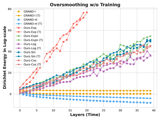
(a) Effects of Training on Oversmoothing

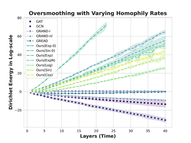
(b) Effects of Homophily on Oversmoothing

Figure 1: The left figure presents a comparative analysis of the Dirichlet energy for several diffusion-based GNNs, including GRAND-l, GRAND-nl, and Ours (Exp, Expn, Log, Sin, Cos), with (T) and without training, over increasing network depths; The right figure displays the effects of homophily level on oversmoothing. Error bands represent the variance in Dirichlet energy across different homophily levels, indicating each model’s sensitivity to homophily.

See proofs in Appendix B.3. In reference to Section 5.2, it has been established that the Markov process denoted as $\mathbf{X}$, characterized by the generator $\mathcal{A}$, will ultimately attain ergodicity across the entire state space. The probability measure $\mu(u)$, representing the likelihood of being in state $u\in\mathcal{V}$, remains unchanged, thereby causing different node features to converge towards a common value, which results in the oversmoothing phenomenon. However, the killing process $\tilde{\mathbf{X}}$ follows a distinct trajectory, as it transitions into a non-operational state, known as the “dead state,” after an unpredictable duration $\tau$. This behavior prevents it from achieving ergodicity throughout the state space and impedes the convergence of node features. It is worth noting that a similar concept is employed in the gating mechanisms frequently utilized in the field of deep learning. In fact, Rusch et al. (2023) has applied this gating mechanism to effectively address the oversmoothing problem.

5.4 Connection to Existing Work

In the context of discrete Graph Neural Networks (GNNs), the process of feature propagation can be intuitively likened to a random walk occurring on the graph structure. Zhao et al. (2022) conducted an extensive investigation into the oversmoothing problem prevalent in classical GNN models like GCN and GAT. This analysis was conducted using discrete-time Markov chains on graphs. Additionally, Thorpe et al. (2022) delved into the oversmoothing issue within the GRAND framework, employing discrete-time random walks for their study.

The probabilistic interpretation presented in this section can be seen as a broader extension of the insights derived from the discrete setting. Our research endeavors further delve into continuous-time Markov processes, with a particular emphasis on exploring the intricate relationships between stochastic processes, operator semigroups, and graph diffusion equations.

6 Experimental Verification

This section presents empirical experiments designed to validate the theoretical analysis of the oversmoothing problem in graph diffusion. Our objectives are twofold: (1) Verification of oversmoothing: We empirically demonstrate the oversmoothing phenomenon in certain graph diffusion structures as theorized, alongside testing a proposed method aimed at mitigating this issue in scenarios both with and without training, and across datasets characterized by differing levels of homophily; (2) Comparative Performance Analysis: The proposed method is evaluated against standard baselines in node classification benchmarks to illustrate its effectiveness in improving performance.

6.1 Specification on Ergodicity Breaking Terms

Following Theorem 4.5, we propose the following ergodicity breaking terms $\mathcal{C}$ w.r.t. the elementary function based on the attention matrix $A$:

• Negative exponential: $e^{-A}=\sum_{n=0}^{\infty}\frac{(-1)^{n}}{n!}A^{n}$;

• Exponential: $e^{A}=\sum_{n=0}^{\infty}\frac{1}{n!}A^{n}$;

• Logarithm: $\log{(I+A)}=\sum_{n=1}^{\infty}\frac{(-1)^{n-1}}{n}A^{n}$;

• Sine: $\sin{A}=\sum_{n=0}^{\infty}\frac{(-1)^{n}}{(2n+1)!}A^{2n+1}$;

• Cosine: $\cos{A}=\sum_{n=0}^{\infty}\frac{(-1)^{n}}{(2n)!}A^{2n}$.

In the implementation level, we truncate the series by $N\in\mathbb{N}^{+}$, resulting breaking terms with different orders.

Table 1: Node-classification results. Top three models are coloured by First, Second, Third

	Texas	Wisconsin	Cornell	Film	Squirrel	Chameleon	Citeseer	Pubmed	Cora
Hom level	0.11	0.21	0.30	0.22	0.22	0.23	0.74	0.80	0.81
PairNorm	$60.27\pm 4.34$	$48.43\pm 6.14$	$58.92\pm 3.15$	$27.40\pm 1.24$	$50.44\pm 2.04$	$62.74\pm 2.82$	$73.59\pm 1.47$	$87.53\pm 0.44$	$85.79\pm 1.01$
GraphSAGE	$82.43\pm 6.14$	$81.18\pm 5.56$	$75.95\pm 5.01$	$34.23\pm 0.99$	$41.61\pm 0.74$	$58.73\pm 1.68$	$76.04\pm 1.30$	$88.45\pm 0.50$	$86.90\pm 1.04$
GCN	$55.14\pm 5.16$	$51.76\pm 3.06$	$60.54\pm 5.30$	$27.32\pm 1.10$	$53.43\pm 2.01$	$64.82\pm 2.24$	$76.50\pm 1.36$	$88.42\pm 0.50$	$86.98\pm 1.27$
GAT	$52.16\pm 6.63$	$49.41\pm 4.09$	$61.89\pm 5.05$	$27.44\pm 0.89$	$40.72\pm 1.55$	$60.26\pm 2.50$	$76.55\pm 1.23$	$87.30\pm 1.10$	$86.33\pm 0.48$
CGNN	$71.35\pm 4.05$	$74.31\pm 7.26$	$66.22\pm 7.69$	$35.95\pm 0.86$	$29.24\pm 1.09$	$46.89\pm 1.66$	${\color[rgb]{0,0,0}76.91\pm 1.81}$	$87.70\pm 0.49$	$87.10\pm 1.35$
GRAND	$75.68\pm 7.25$	$79.41\pm 3.64$	$74.59\pm 4.04$	$35.62\pm 1.01$	$40.05\pm 1.50$	$54.67\pm 2.54$	$76.46\pm 1.77$	$89.02\pm 0.51$	$87.36\pm 0.96$
Sheaf	${85.40\pm 6.07}$	${\color[rgb]{1,0,0}89.41\pm 4.74}$	${\color[rgb]{1,0,0}84.86\pm 4.71}$	${\color[rgb]{1,0,0}37.81\pm 1.15}$	${\color[rgb]{0,0,0}56.34\pm 1.32}$	$67.71\pm 1.22$	$76.70\pm 1.57$	$89.49\pm 0.40$	$86.90\pm 1.13$
GRAFF	$84.32\pm 5.51$	${\color[rgb]{0,0,0}85.68\pm 3.40}$	$71.08\pm 3.64$	$35.55\pm 1.20$	${\color[rgb]{0,0,1}57.60\pm 1.42}$	${\color[rgb]{0,0,0}68.75\pm 1.83}$	${75.27\pm 1.45}$	${89.60\pm 0.40}$	${87.66\pm 0.97}$
GREAD	${84.59\pm 4.53}$	$85.29\pm 4.49$	$73.78\pm 4.53$	$37.59\pm 1.06$	${\color[rgb]{1,0,0}58.62\pm 1.08}$	${\color[rgb]{0,0,1}70.00\pm 1.70}$	$77.09\pm 1.78$	${\color[rgb]{0,0,0}90.01\pm 0.42}$	${\color[rgb]{0,0,0}88.16\pm 0.81}$
Ours-Expn	${\color[rgb]{1,0,0}88.65\pm 2.64}$	${\color[rgb]{0,0,1}88.82\pm 3.62}$	${\color[rgb]{0,0,0}76.48\pm 2.71}$	${\color[rgb]{0,0,1}37.79\pm 0.86}$	${\color[rgb]{0,0,0}50.83\pm 1.69}$	${\color[rgb]{0,0,0}69.74\pm 1.26}$	${\color[rgb]{1,0,0}77.48\pm 1.26}$	${\color[rgb]{1,0,0}90.08\pm 0.49}$	${\color[rgb]{0,0,1}88.31\pm 0.85}$
Ours-Exp	${\color[rgb]{0,0,0}84.06\pm 4.59}$	${\color[rgb]{1,.5,0}87.64\pm 3.51}$	${\color[rgb]{0,0,0}77.57\pm 3.83}$	${\color[rgb]{0,0,0}37.37\pm 1.17}$	${\color[rgb]{0,0,0}50.03\pm 1.90}$	${\color[rgb]{0,0,0}69.41\pm 1.15}$	${\color[rgb]{0,0,0}76.75\pm 1.76}$	${\color[rgb]{0,0,0}89.92\pm 0.37}$	${\color[rgb]{0,0,0}87.97\pm 1.09}$
Ours-Log	${\color[rgb]{0,0,1}87.03\pm 5.24}$	${\color[rgb]{0,0,0}86.67\pm 2.60}$	${\color[rgb]{0,0,1}78.11\pm 3.90}$	${\color[rgb]{0,0,0}37.55\pm 0.80}$	${\color[rgb]{0,0,0}54.75\pm 1.57}$	${\color[rgb]{1,.5,0}70.75\pm 1.39}$	${\color[rgb]{0,0,0}77.07\pm 1.60}$	${\color[rgb]{0,0,1}90.02\pm 0.38}$	${\color[rgb]{0,0,0}88.07\pm 1.24}$
Ours-Sin	${\color[rgb]{0,0,0}85.41\pm 5.94}$	${\color[rgb]{0,0,0}87.26\pm 5.21}$	${\color[rgb]{1,.5,0}77.84\pm 3.15}$	${\color[rgb]{0,0,0}37.64\pm 0.89}$	${\color[rgb]{1,.5,0}56.35\pm 1.89}$	${\color[rgb]{1,0,0}70.88\pm 1.58}$	${\color[rgb]{1,.5,0}77.13\pm 0.97}$	${\color[rgb]{1,.5,0}89.98\pm 0.45}$	${\color[rgb]{1,.5,0}88.21\pm 0.94}$
Ours-Cos	${\color[rgb]{1,.5,0}86.21\pm 5.20}$	${\color[rgb]{0,0,0}85.69\pm 4.21}$	${\color[rgb]{0,0,0}77.57\pm 1.73}$	${\color[rgb]{1,.5,0}37.75\pm 0.89}$	${\color[rgb]{0,0,0}52.44\pm 0.81}$	${\color[rgb]{0,0,0}68.18\pm 1.69}$	${\color[rgb]{0,0,1}77.21\pm 1.81}$	${\color[rgb]{0,0,0}89.94\pm 0.39}$	${\color[rgb]{1,0,0}88.33\pm 0.61}$

6.2 Oversmoothing Validation

We first empirically validate the oversmoothing phenomenon as posited in our theoretical analysis. Dirichlet energy is utilized as the primary metric for this purpose, defining as:

$$E\left(H,A\right)=\frac{1}{N}\sum_{u\in\mathcal{V}}\sum_{v\in\mathcal{N}(u)}a(u,v)\left\|h_{u}-h_{v}\right\|^{2}.$$

We adopt the synthetic Cora (Zhu et al., 2020) dataset for our experiments. To contextualize our findings, we compare the following models: GCN (Kipf & Welling, 2017), GAT (Velickovic et al., 2017), GRAND (Chamberlain et al., 2021b), GREAD (Choi et al., 2023) and ergodicity-breaking terms in Sec. 6.1, denoting as Ours-Exp, Ours-ExpN, Ours-Log, Ours-Sin, Ours-Cos. Detailed configurations and further results are in Appendix C.1.

The experimental findings delve into several critical aspects of oversmoothing issues that have been less emphasized in prior research:
Question: Does the training process influence oversmoothing effects?
Answer: Figure 1(a) shows that the training process does not significantly impact the oversmoothing effects in various graph neural network models. Both trained and untrained versions of models such as GRAND-l, GRAND-nl, and the graph diffusion model with ergodicity-breaking terms (Ours-Exp, Ours-ExpN, Ours-Log, Ours-Sin, Ours-Cos) demonstrate similar trends in Dirichlet energy as the network depth increases. This consistency across models, regardless of their training status, suggests that oversmoothing is predominantly a function of the model’s inherent architecture rather than its training.

Question: What’s the impact of varying levels of homophily on oversmoothing?
Answer: Figure 1(b)’s error bands, which illustrate the variance due to different homophily levels, show that some models are more sensitive to homophily changes than others. For instance, models like GAT and GCN, with wider error bands, indicate a higher sensitivity to homophily levels, implying that their performance in managing oversmoothing varies more significantly with changes in homophily. Conversely, certain models from the ‘Ours’ series, characterized by narrower error bands, demonstrate greater stability against oversmoothing across varying homophily levels. This highlights that while some GNN models are robust against homophily variations, others may require careful consideration of the dataset’s homophily characteristics for optimal performance.

6.3 Node Classification

Datasets. We evaluate the performance of our proposed method in comparison with existing GNN architectures. The focus is on both heterophilic and homophilic graph datasets to showcase the model’s versatility and robustness across diverse real-world scenarios. For heterophilic datasets, we utilize six datasets known for their low homophily ratios as identified in (Pei et al., 2020), including Chameleon and Squirrel (Rozemberczki et al., 2021), Film (Tang et al., 2009), Texas, Wisconsin, and Cornell datasets from the WebKB collection. For homophilic datasets, we employ Cora (McCallum et al., 2000), CiteSeer (Sen et al., 2008) and PubMed (Yang et al., 2016). For data splits, we adopt the methodology from (Pei et al., 2020), ensuring consistency and comparability in our evaluations. The performance is gauged in terms of accuracy, with both mean and standard deviation reported. Each experiment is conducted over 10 fixed train/validation/test splits to ensure the reliability and reproducibility of results.

Baselines. Our model is benchmarked against a comprehensive set of GNN architectures, encompassing both traditional models: GCN (Kipf & Welling, 2017), GAT (Velickovic et al., 2017) and GraphSage (Hamilton et al., 2017), and recent ODE-based models: Continuous Graph Neural Networks (CGNN) (Xhonneux et al., 2020), GRAND (Chamberlain et al., 2021b), Sheaf (Bodnar et al., 2022), GRAFF (Di Giovanni et al., 2022) and GREAD (Choi et al., 2023).

Our Method We use the ergodicity breaking terms in Sec. 6.1 with specific truncated orders $N$ and different ODE block, detailed optimal configurations are in Appendix C.2.

Results. The data presented in Table 1 illuminates the comparative efficacy of diverse graph neural network models when applied to datasets characterized by varying degrees of homophily. Notably, the diffusion-based models, augmented with our proposed ergodicity breaking terms, demonstrate remarkable robustness and adaptability, emerging as the top-performing models on 5 out of 9 datasets. Furthermore, they secure the second position on 7 out of 9 datasets, consistently achieving top-three performance overall. Particularly noteworthy is their exceptional performance on datasets with a high homophily level, such as Citeseer, Pubmed, and Cora, as well as on the Texas dataset, which exhibits the lowest level of homophily. The ‘Ours’ suite of models demonstrates commendable performance by attaining the highest ranks across all these datasets. The ‘Ours’ suite of models demonstrates commendable performance by attaining the highest ranks across all these datasets.

7 Conclusions

This paper presents a unified framework rooted in operator semigroup theory to address oversmoothing in diffusion-based GNNs. Grounded in this framework, the introduced versatile ergodicity-breaking condition can incorporate previous research and offer universal guidance for countering oversmoothing. Empirical validation demonstrates its effectiveness in enhancing node classification performance. Our probabilistic interpretation establishes a vital connection with existing literature and enhances the comprehensiveness of our approach.

Broader Impact

Our contributions to the field of diffusion-based Graph Neural Networks (GNNs) have broad implications for both theoretical research and practical applications in data science and artificial intelligence. By introducing a novel framework grounded in operator semigroup theory, we address the pervasive issue of oversmoothing, thereby enhancing the effectiveness and interpretability of GNNs. The introduction of an ergodicity-breaking condition, validated by both synthetic and real-world data, extends the utility of GNNs beyond traditional boundaries, offering new avenues for analysis and application. Our probabilistic interpretation further bridges theoretical gaps, fostering a deeper understanding of GNN dynamics. This work not only advances the state-of-the-art in GNN methodologies but also expands their applicability in solving complex networked problems, marking a significant step forward in the development of more robust and versatile AI systems.

Appendix A Proofs for Sec. 3 and 4

A.1 Proof of Proposition 3.2

Semigroup $P_{t}$ induced by the operator $\mathcal{A}$ satisfies: $\frac{\partial P_{t}}{\partial t}=\mathcal{A}P_{t}=P_{t}\mathcal{A},$ then it can be expressed as: $P_{t}=e^{t\mathcal{A}}.$ For $f:\mathcal{V}\rightarrow\mathcal{R}^{n}$, we define $Q=A-I$, then $P_{t}f=e^{t\mathcal{A}}f=e^{tQ}f$. Since A is normalized, $Q=(q_{uv})_{u,v\in\mathcal{V}}$ is a Q-matrix satisfying the following conditions: (i) $0\leq-q_{ii}<\infty$ for all $i$; (ii) $q_{ij}\geq 0$ for all $i\neq j$; (iii) $\sum_{j\in I}q_{ij}=0$ for all $i$. We state a lemma without proof, which describes the relationship between $Q$ and operator $P_{t}$:

Lemma A.1 (Theorem 2.1.2 of (Norris, 1998) ).

A matrix $Q$ on a finite set is a $Q$-matrix if and only if $P_{t}=e^{tQ}$ is a stochastic matrix for all $t\geq 0$.

Proof of proposition 3.2.

Lemma A.1 demonstrated that $P_{t}$ is a stochastic matrix adhere to: $0\leq p_{ij}<\infty$ , $\sum_{j\in I}p_{ij}=1$ for all $i$, leading to (i) and (ii). ∎

A.2 Proof of Theorem 4.3

Lemma A.2.

Measure $\mu$ with respect to operator $\mathcal{A}$ is an positive eigenvector of the transpose of $A=(a(u,v))_{u,v\in\mathcal{V}}$ with eigenvalue 1.

Proof.

Suppose $\mu$ is an eigenvector of $A^{T}$ with eigenvalue 1, then $A^{T}\mu=\mu$ and $\mu(v)=\sum_{u}a(u,v)\mu(u)$

$$\sum_{u\in\mathcal{V}}\mathcal{A}f(u)\mu(u) =\sum_{u}\sum_{v}a(u,v)(f(v)-f(u))\mu(u)$$

$$=\sum_{u}\sum_{v}a(u,v)f(v)\mu(u)-\sum_{u}f(u)\mu(u)$$

$$=\sum_{v}\sum_{u}a(u,v)\mu(u)f(v)-\sum_{u}f(u)\mu(u)$$

$$=\sum_{v}f(v)\mu(v)-\sum_{u}f(u)\mu(u)$$

$$=0.$$

This proves $\mu$ is invariant with respect to operator $\mathcal{A}$. And positivity of $\mu$ is ensured by the Perron-Frobenius theorem. ∎

We first consider operator $\mathcal{A}$ define in Eq.(6) is self-adjoint, that is, $\mathcal{A}$ is equal to its adjoint operator $\mathcal{A}^{*}$. To be specific, $\langle\mathcal{A}f,g\rangle=\langle f,\mathcal{A}g\rangle$, for every $f,g\in C(\mathcal{V})$, where inner product $\langle f,g\rangle:=\int_{\mathcal{V}}fg\mathrm{d}\mu$.

Proof of Theorem 4.3.

Since $\mathcal{G}$ is a connected graph, then $A=(a(u,v))_{u,v\in\mathcal{V}}$ is irreducible, that is, for every pair of vertices $(u,v)\in\mathcal{V}\times\mathcal{V}$, there exists a path $(u=u_{0},u_{1},\ldots,u_{k-1},u_{k}=v)$ in $\mathcal{V}$, such that for $i=0,1,\ldots,k-1$, $a(u_{i},u_{i+1})>0$. Equivalently, $A$ is not similar via a permutation to a block upper triangular matrix.

From Perron-Frobenius theorem for irreducible matrices, we know that the maximal eigenvalue $\lambda_{0}=0$ of $\mathcal{A}$ is unique (algebra multiplicity is $1$) and the geometric multiplicity of $\lambda_{0}$ is $1$, that is, the corresponding normalized eigenfunction of $\lambda_{0}$ is unique, noted as $f$. Consider

$$\langle\mathcal{A}f,f\rangle =\sum_{u\in\mathcal{V}}\left[\sum_{v\in\mathcal{V}}a(u,v)(f(v)-f(u))\right]f(u)\mu(u)$$

$$=\frac{1}{2}\left[\sum_{u\in\mathcal{V}}\sum_{v\in\mathcal{V}}a(u,v)(f(v)-f(u))f(u)\mu(u)+\sum_{v\in\mathcal{V}}\sum_{u\in\mathcal{V}}a(v,u)(f(u)-f(v))f(v)\mu(v)\right]$$

$$=\frac{1}{2}\sum_{u\in\mathcal{V}}\sum_{v\in\mathcal{V}}a(u,v)\left[(f(v)-f(u))f(u)+(f(u)-f(v))f(v)\right]\mu(u)$$

$$=-\frac{1}{2}\sum_{u\in\mathcal{V}}\sum_{v\in\mathcal{V}}a(u,v)(f(u)-f(v))^{2}\mu(u),$$

$f$ is the corresponding normalized eigenfunction of $\lambda_{0}=0$, that is, $\mathcal{A}f=0$, then $\langle\mathcal{A}f,f\rangle=0$. Therefore

$$f(u)=f(v):=c,\quad\forall u,v\in\mathcal{V}.$$

Notice the uniqueness of $f$, operator $\mathcal{A}$ is ergodic. ∎

A.3 Proof of Theorem 4.4

Proof.

Since operator $\mathcal{A}$ is self-adjoint, consider the spectral decomposition of the generator $\mathcal{A}$

$$\mathcal{A}f=\sum_{k=0}^{N}\lambda_{k}E_{\lambda_{k}}f=\sum_{k=0}^{N}\lambda_{k}f_{\lambda_{k}}e_{\lambda_{k}},$$

where $\lambda_{k},k=0,1,\ldots,N$ are the eigenvalues of $\mathcal{A}$, $e_{\lambda_{k}}$ are corresponding normalized eigenfunctions of $\lambda_{k}$, $E_{\lambda_{k}}$ are corresponding projection operators of $\lambda_{k}$, and $f_{\lambda_{k}}$ is the projection of $f$ related to $e_{\lambda_{k}}$ . For $t\geq 0$,

$$P_{t}f=e^{t\mathcal{A}}f=\sum_{k=0}^{N}e^{\lambda_{k}t}f_{\lambda_{k}}e_{\lambda_{k}}.$$

Since graph $\mathcal{G}$ is connected, Perron-Frobenius theorem implies that eigenvalues of $\mathcal{A}$ satisfy $0=\lambda_{0}>\lambda_{1},\ldots,\lambda_{N}$. As $t\rightarrow\infty$,

$$P_{t}f(u)\rightarrow f_{\lambda_{0}}e_{\lambda_{0}}.$$

Since operator $\mathcal{A}$ is ergodic, $f_{\lambda_{0}}e_{\lambda_{0}}$ is a constant. Notice

$$\mathcal{A}(\sum_{u\in\mathcal{V}}f(u)\mu(u))=\sum_{u\in\mathcal{V}}\mathcal{A}f(u)\mu(u)=0,$$

therefore $f_{\lambda_{0}}e_{\lambda_{0}}=\sum_{u\in\mathcal{V}}f(u)\mu(u).$ ∎

Since $P_{t}f$ converges to the eigenspace corresponding to the eigenvalue $\lambda_{0}=0$, once the generator is not ergodic, the projection of function $f\in\mathscr{L}^{2}(\mathcal{V},\mu)$ onto the eigenspace corresponding to the eigenvalue $0$ is not constant. Therefore, $\lim\limits_{t\rightarrow\infty}P_{t}f$ is not constant. That means not oversmoothing.

If $A$ is not symmetric, while for every pair of vertices $(u,v)\in\mathcal{V}\times\mathcal{V}$,

$$\mu(u)a(u,v)=\mu(v)a(v,u),$$

which is so called detailed balance condition, we say $\mu$ is reversible. We can simply symmetrize $A$ by

$$\tilde{a}(u,v):=\sqrt{\mu(u)}a(u,v)\frac{1}{\sqrt{\mu(v)}}.$$

Consider the symmertrized operator $\tilde{\mathcal{A}}$ satisfying : $\tilde{\mathcal{A}}f(u)=\sum_{v\in\mathcal{V}}\tilde{a}(u,v)(f(v)-f(u))$, we can obtain similar conclusions.

A.4 Proof of Theorem 4.5

Proof.

Let $f_{c}\in\mathscr{L}^{2}(\mathcal{V},\mu)$ such that

$$(\mathcal{A}+\mathcal{C})f_{c}(u)=\sum_{v\in\mathcal{V}}a(u,v)(f_{c}(v)-f_{c}(u))+\mathcal{C}f_{c}(u)=0.$$

We assume that $\mathcal{A}+\mathcal{C}$ is ergodic, that is, $f_{c}$ is a constant. Let $f_{c}(u)=b$, for all $u\in\mathcal{V}$. Then

$$(\mathcal{A}+c)f_{c}(u)=\sum_{v\in\mathcal{V}}a(u,v)(b-b)+\mathcal{C}b=\mathcal{C}b.$$

Since $\mathcal{A}b=\sum_{v\in\mathcal{V}}a(u,v)(b-b)=0$, $\mathcal{C}b\neq 0$. It is contradict to $(\mathcal{A}+\mathcal{C})f_{c}(u)=0$. Therefore $\mathcal{A}+\mathcal{C}$ is not ergodic.

∎

Appendix B Proofs for Sec. 5

B.1 Proof of Theorem 5.1

Proof.

From the definition of generator,

$$\mathcal{A}h_{i}(u,t) =\lim\limits_{r\rightarrow 0^{+}}\frac{P_{r}h_{i}(u,t)-h_{i}(u,t)}{r}$$

$$=\lim\limits_{r\rightarrow 0^{+}}\frac{\mathbb{E}^{u}[h_{i}(\mathbf{X}_{r},t)]-h_{i}(u,t)}{r}$$

$$=\lim\limits_{r\rightarrow 0^{+}}\frac{\mathbb{E}^{u}[\mathbb{E}^{\mathbf{X}_{r}}[f_{i}(\mathbf{X}_{t})]]-\mathbb{E}^{u}[f_{i}(\mathbf{X}_{t})]}{r}.$$

Let $\{\mathscr{F}_{t}\}$ be the right continuous $\sigma$-algebra filtration with respect to which $\mathbf{X}_{t}$ is adapted. From Chapman–Kolmogorov equation (or Markov property),

$$\mathbb{E}^{\mathbf{X}_{r}}[f_{i}(\mathbf{X}_{t})]=\mathbb{E}^{u}[f_{i}(\mathbf{X}_{t+r})|\mathscr{F}_{r}].$$

Then,

$$\mathcal{A}h_{i}(u,t) =\lim\limits_{r\rightarrow 0^{+}}\frac{\mathbb{E}^{u}[\mathbb{E}^{u}[f_{i}(\mathbf{X}_{t+r})|\mathscr{F}_{r}]]-\mathbb{E}^{u}[f_{i}(\mathbf{X}_{t})]}{r}$$

$$=\lim\limits_{r\rightarrow 0^{+}}\frac{\mathbb{E}^{u}[f_{i}(\mathbf{X}_{t+r})]-\mathbb{E}^{u}[f_{i}(\mathbf{X}_{t})]}{r}$$

$$=\lim\limits_{r\rightarrow 0^{+}}\frac{h_{i}(u,t+r)-h_{i}(u,t)}{r}$$

$$=\frac{\partial h_{i}(u,t)}{\partial t}.$$

Further, $\mathbb{E}^{u}[f_{i}(\mathbf{X}_{0})]=f_{i}(u)=h_{i}(u,0)$. Therefore, $\mathbb{E}^{u}[f_{i}(\mathbf{X}_{t})]$ is the solution of Cauchy problem ((7)). ∎

B.2 Proof of Theorem 5.2

Proof.

Fix $h>0$ and consider the h-skeleton $\mathbf{Z}_{n}:=\mathbf{X}_{nh}$ of $\mathbf{X}$. Since

$$\mathbb{P}(\mathbf{Z}_{n+1}=u_{n+1}|\mathbf{Z}_{0}=u_{0},\ldots,\mathbf{Z}_{n}=u_{n})=p(h,u_{n},u_{n+1}),$$

h-skeleton chain $\mathbf{Z}_{n}$ is discrete time Markov chain with transition matrix $P(h)$. Since $\mathcal{G}$ is a finite connected graph, for all $u,v\in\mathcal{V}$, there exists some $t$, such that $p(t,u,v)>0$. Therefore $\mathbf{Z}_{n}$ is irreducible and aperiodic. From classic result of discrete time Markov chain(Norris, 1998), there exists a unique invariant measure $\mu$, for all $u,v\in\mathcal{V}$

$$p(nh,u,v)\rightarrow\mu(v),\quad n\rightarrow\infty.$$

For fixed state $u$,

$$|p(t+h,u,v)-p(t,u,v)| =|\sum_{k\in\mathcal{V}}p(h,u,k)p(t,k,v)-p(t,u,v)|$$

$$=|\sum_{k\neq u}p(h,u,k)p(t,k,v)-(1-p(h,u,u))p(t,u,v)|$$

$$\leq 1-p(h,u,u)\leq\mathbb{P}(J_{1}\leq h|\mathbf{X}_{0}=u)=1-e^{h\cdot(a(u,u)-1)}.$$

so given $\epsilon>0$ we can find $h>0$ such that

$$|p(t+h,u,v)-p(t,u,v)|\leq 1-e^{s\cdot(a(u,u)-1)}<\frac{\epsilon}{2},\quad 0\leq s\leq h$$

and find $N\in\mathbb{N}$ such that

$$|p(nh,u,v)-\mu(v)|<\frac{\epsilon}{2},\quad n>N.$$

For $t>Nh$ we have $nh\leq t<(n+1)h$ for some $n>N$ and

$$|p(t,u,v)-\mu(v)|\leq|p(t,u,v)-p(nh,u,v)|+|p(nh,u,v)-\mu(v)|<\epsilon.$$

Hence

$$p(t,u,v)\rightarrow\mu(v),\quad t\rightarrow\infty.$$

∎

B.3 Proof of Theorem 5.3

Proof.

We first show that $\tilde{\mathbf{X}}$ is a Markov process. For all $u\in\mathcal{V}$,

$$\mathbb{P}(\tilde{\mathbf{X}}_{t+s}=u\;|\;\mathscr{F}_{s}) =\mathbb{P}(\mathbf{X}_{t+s}=u,\tau>t+s\;|\;\mathscr{F}_{s})$$

$$=\mathbb{P}(\mathbf{X}_{t+s}=u,\tau>t+s\;|\;\mathbf{X}_{s})\mathbf{1}_{\tilde{\mathbf{X}}_{s}\neq\partial}$$

$$=\mathbb{P}(\tilde{\mathbf{X}}_{t+s}=u\;|\;\tilde{\mathbf{X}}_{s})\mathbf{1}_{\tilde{\mathbf{X}}_{s}\neq\partial}.$$

On the other hand,

$$\mathbb{P}(\tilde{\mathbf{X}}_{t+s}=\partial\;|\;\mathscr{F}_{s}) =\mathbb{P}(\tau\leq t+s\;|\;\mathscr{F}_{s})$$

$$=\mathbb{P}(\tau\leq s\;|\;\mathscr{F}_{s})+\mathbb{P}(s<\tau\leq t+s\;|\;\mathscr{F}_{s})$$

$$=\mathbf{1}_{\tau\leq s}+\mathbb{P}(s<\tau\leq t+s\;|\;\mathscr{F}_{s})$$

$$=\mathbf{1}_{\tilde{\mathbf{X}}_{s}=\partial}+\mathbb{P}(s<\tau\leq t+s\;|\;\tilde{\mathbf{X}}_{s})\mathbf{1}_{\tilde{\mathbf{X}}_{s}\neq\partial}$$

$$=\mathbf{1}_{\tilde{\mathbf{X}}_{s}=\partial}+\mathbb{P}(\tilde{\mathbf{X}}_{t+s}=\partial\;|\;\tilde{\mathbf{X}}_{s})\mathbf{1}_{\tilde{\mathbf{X}}_{s}\neq\partial}$$

$$=\mathbb{P}(\tilde{\mathbf{X}}_{t+s}=\partial\;|\;\tilde{\mathbf{X}}_{s}).$$

Thus $\tilde{\mathbf{X}}$ is a Markov process. Moreover, since $\mathcal{V}$ is finite, $\tilde{\mathbf{X}}$ is a strong Markov process. We next calculate the generators of $\tilde{\mathbf{X}}$. We need the following lemma:

Lemma B.1 (The Feynman-Kac formula, Theorem 8.2.1 of Oksendal (2013)).

Let $f\in C_{0}^{2}(\mathbb{R}^{n})$ and $q\in C(\mathbb{R}^{n})$. Assume that $q$ is lower bounded. Put

$$v(t,x)=\mathbb{E}^{x}\left[\exp\left(-\int_{0}^{t}q(\xi_{s})\mathrm{d}s\right)f(\xi_{t})\right].$$

Then

$$\frac{\partial v}{\partial t}=Av-qv,\quad v(0,x)=f(x),\quad t>0,\;x\in\mathbb{R}^{n},$$

where $A$ is generator of diffusion process $\xi$.

For bounded continuous functions $f$,

$$\mathbb{E}^{u}[f(\tilde{\mathbf{X}}_{t})]=\mathbb{E}^{u}[f(\mathbf{X}_{t})\cdot\mathbf{1}_{[0,\tau)}(t)]=\mathbb{E}^{u}[f(\mathbf{X}_{t})\cdot e^{\int_{0}^{t}c(\mathbf{X}_{s})\mathrm{d}s}],$$

where $c(u)=-\lim\limits_{t\rightarrow 0^{+}}\frac{1}{t}\mathbb{P}(\tau\leq t|\mathbf{X}_{0}=u)$. Then, by lemma B.1,

$$\lim_{t\rightarrow 0^{+}}\frac{\mathbb{E}^{u}[f(\tilde{\mathbf{X}}_{t})]-f(u)}{t}=\mathcal{A}f(u)+c(u)f(u).$$

That is, the generator of $\tilde{\mathbf{X}}$ is

$$\tilde{\mathcal{A}}=\mathcal{A}+c(u).$$

∎

Appendix C Experimental Details and Further Results

C.1 Configurations and Results for Oversmoothing

Synthetic Cora Dataset The Synthetic Cora dataset, as introduced by Zhu et al. (2020), is a variant of the well-known Cora dataset tailored for graph neural network (GNN) experiments. This dataset is characterized by its homophily index, which ranges from 0 to 1. Homophily in this context refers to the tendency of nodes in the graph to be connected to other nodes with similar features or labels. A homophily index of 0 indicates no homophily (i.e., connections are completely independent of node labels), while an index of 1 signifies perfect homophily (i.e., nodes are only connected to others with the same label). This range allows for controlled experiments to understand the behavior of GNNs under varying degrees of homophily, which is crucial for assessing the robustness and adaptability of different models. We provide the detailed information of the synthetic Cora networks in Table 2.

Table 2: Detailed characteristics of the Synthetic Cora dataset across various homophily levels. Each homophily level maintains identical counts of features (1,433), nodes (1,480), edges (5,936), and classes (5), ensuring consistent structural properties while varying node similarity.

Homophily	Avg. Degree	Max. Degree	Min. Degree
0.0	3.98	84.33	1.67
0.1	3.98	71.33	2.00
0.2	3.98	73.33	1.67
0.3	3.98	70.00	2.00
0.4	3.98	77.67	2.00
0.5	3.98	76.33	2.00
0.6	3.98	76.00	1.67
0.7	3.98	67.67	2.00
0.8	3.98	58.00	1.67
0.9	3.98	58.00	1.67
1.0	3.98	51.00	2.00

Configurations For Figure 1 and Further Results For all ergodicity-breaking terms, we use a first-order truncation for ergodicity-breaking terms within our proposed models: Ours-Exp, Ours-ExpN, Ours-Log, Ours-Sin, and Ours-Cos. We further show the comprehensive results of oversmoothing with different homophily levels and ergodicity-breaking orders in Figure 2.

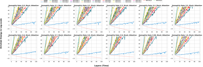
(a) Dirichlet Energy Demonstration For Attention Block With Training

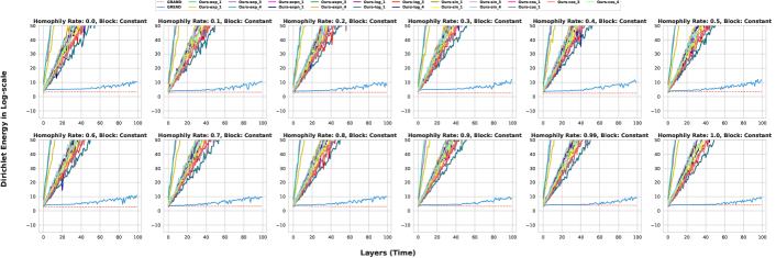
(b) Dirichlet Energy Demonstration For Constant Block With Training

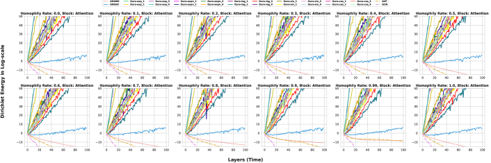
(c) Dirichlet Energy Demonstration For Attention Block Without Training

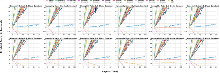
(d) Dirichlet Energy Demonstration For Constant Block Without Training

Figure 2: Comprehensive Demonstration of the Dirichlet energy for extensive diffusion-based GNNs, including GRAND-l, GRAND-nl, and our method (Exp, Expn, Log, Sin, Cos) with different orders {1,2,3,4} over increasing network depths and homophily levels on synthetic Cora dataset.

C.2 Configurations for Node Classification Tasks

All experiments reported in this work were conducted within a uniform computational environment to ensure reproducibility and consistency of results. The specifications of the environment are as follows: Operating System: Ubuntu 18.04 LTS; Programming Language: Python 3.10.4; Deep Learning Framework: PyTorch 2.0.1; Graph Neural Network Library: PyTorch Geometric 2.4.0; Differential Equation Solver: TorchDiffEq 0.2.3; GPU Computing: CUDA 11.7; Processor: AMD EPYC 7542 32-Core Processor; Graphics Card: NVIDIA RTX 3090.

The ergodicity-breaking terms introduced in Sec. 6.3 were configured with specific truncated orders N. The optimal hyperparameters for each term were meticulously tuned based on the performance of the GREAD (Choi et al., 2023). The optimal configurations are systematically listed in Tables 3-7. Each table corresponds to one of the ergodicity-breaking terms and includes the tuned parameters.

Table 3: Best hyperparameters of Exponential Ergodicity Breaking Terms

Hyperparameters	Texas	Wisconsin	Cornell	Film	Squirrel	Chameleon	Cora	Citeseer	PubMed
Order	1	1	2	2	1	3	2	1	2
Block	Attention	Constant	Constant	Constant	Constant	1	1	2	3
$\alpha$	SC	SC	SC	VC	VC	VC	SC	VC	SC
$\beta$	SC	SC	SC	VC	VC	VC	SC	SC	VC
learning rate	0.0100	0.0154	0.0082	0.0079	0.0171	0.0068	0.0105	0.0024	0.0108
weight decay	0.0247	0.0090	0.0280	0.0014	0.0000	0.0060	0.0146	0.0005
input dropout	0.47	0.54	0.49	0.42	0.52	0.68	0.53	0.50	0.36
dropout	0.48	0.48	0.32	0.65	0.09	0.05	0.45	0.47	0.26
dim(H)	256	256	64	64	128	256	128	256	128
step size $\tau$	1.0	0.24	0.25	0.1	0.72	1.72	0.5	0.45	0.1
time $T$	1.461	1.85	0.115	0.2	5.725	1.91	3.575	2.28	1
ODE solver	Euler	Euler	RK4	Euler	Euler	Euler	RK4	Euler	RK4

Table 4: Best hyperparameters of Negative exponential Ergodicity Breaking Term

Hyperparameters	Texas	Wisconsin	Cornell	Film	Squirrel	Chameleon	Cora	Citeseer	PubMed
Order	1	1	2	3	1	3	1	3	1
Block	Attention	Attention	Attention	Attention	Constant	1	1	2	3
$\alpha$	SC	SC	VC	VC	VC	VC	SC	VC	SC
$\beta$	SC	VC	VC	SC	VC	VC	SC	VC	VC
learning rate	0.0100	0.0154	0.0082	0.0079	0.0171	0.0068	0.0105	0.0024	0.0108
weight decay	0.0247	0.0090	0.0280	0.0014	0.0000	0.0060	0.0146	0.0005
input dropout	0.47	0.54	0.49	0.42	0.52	0.68	0.53	0.50	0.36
dropout	0.48	0.48	0.32	0.65	0.09	0.05	0.45	0.47	0.26
dim(H)	64	256	64	32	256	256	128	128	64
step size $\tau$	1.0	0.2	0.2	0.1	0.94	1.66	0.25	0.5	0.8
time $T$	1.461	1.6	0.135	0.35	5.9	1.9	3.49	2.38	1.74
ODE solver	Euler	RK4	RK4	Euler	Euler	RK4	RK4	Euler	RK4

Table 5: Best hyperparameters of Logarithm Ergodicity Breaking Term

Hyperparameters	Texas	Wisconsin	Cornell	Film	Squirrel	Chameleon	Cora	Citeseer	PubMed
Order	2	2	3	1	1	1	2	2	2
Block	Constant	Constant	Constant	Constant	Constant	1	1	2	3
$\alpha$	SC	SC	SC	VC	VC	VC	VC	VC	SC
$\beta$	SC	SC	VC	VC	VC	VC	SC	VC	SC
learning rate	0.0100	0.0154	0.0082	0.0079	0.0171	0.0068	0.0105	0.0024	0.0108
weight decay	0.0247	0.0090	0.0280	0.0014	0.0000	0.0060	0.0146	0.0005
input dropout	0.47	0.54	0.49	0.42	0.52	0.68	0.53	0.50	0.36
dropout	0.48	0.48	0.32	0.65	0.09	0.05	0.45	0.47	0.26
dim(H)	64	128	256	32	128	256	64	64	128
step size $\tau$	1.0	0.22	0.24	0.16	0.8	1.62	0.5	0.45	0.8
time $T$	1.461	1.8	0.13	0.45	5.925	1.99	3.79	2.26	1.74
ODE solver	Euler	RK4	Euler	RK4	Euler	Euler	RK4	Euler	RK4

Table 6: Best hyperparameters of Sine Ergodicity Breaking Term

Hyperparameters	Texas	Wisconsin	Cornell	Film	Squirrel	Chameleon	Cora	Citeseer	PubMed
Order	3	3	3	1	1	1	1	2	3
Block	Constant	Attention	Constant	Attention	Constant	1	1	2	3
$\alpha$	SC	SC	VC	SC	SC	VC	VC	VC	SC
$\beta$	VC	VC	VC	VC	VC	VC	SC	VC	VC
learning rate	0.0100	0.0154	0.0082	0.0079	0.0171	0.0068	0.0105	0.0024	0.0108
weight decay	0.0247	0.0090	0.0280	0.0014	0.0000	0.0060	0.0146	0.0005
input dropout	0.47	0.54	0.49	0.42	0.52	0.68	0.53	0.50	0.36
dropout	0.48	0.48	0.32	0.65	0.09	0.05	0.45	0.47	0.26
dim(H)	32	64	32	128	128	256	128	256	256
step size $\tau$	1.0	0.22	0.21	0.16	0.98	1.66	0.5	0.45	0.8
time $T$	1.461	1.875	0.125	0.3	5.925	1.99	3.57	2.24	1.74
ODE solver	Euler	Euler	Euler	RK4	Euler	Euler	RK4	Euler	RK4

Table 7: Best hyperparameters of Cosine Ergodicity Breaking Term

Hyperparameters	Texas	Wisconsin	Cornell	Film	Squirrel	Chameleon	Cora	Citeseer	PubMed
Order	1	1	2	2	1	3	1	2	3
Block	Attention	Attention	Attention	Attention	Constant	1	1	2	3
$\alpha$	SC	SC	VC	VC	SC	SC	VC	VC	VC
$\beta$	VC	SC	VC	SC	VC	VC	VC	VC	SC
learning rate	0.0100	0.0154	0.0082	0.0079	0.0171	0.0068	0.0105	0.0024	0.0108
weight decay	0.0247	0.0090	0.0280	0.0014	0.0000	0.0060	0.0146	0.0005
input dropout	0.47	0.54	0.49	0.42	0.52	0.68	0.53	0.50	0.36
dropout	0.48	0.48	0.32	0.65	0.09	0.05	0.45	0.47	0.26
dim(H)	64	64	32	64	128	256	128	256	64
step size $\tau$	1.0	0.26	0.16	0.1	0.98	1.74	0.25	0.5	0.8
time $T$	1.44	1.625	0.12	0.125	5.625	1.71	3.98	2.24	1.74
ODE solver	Euler	RK4	RK4	RK4	Euler	RK4	Euler	RK4	RK4

References

- Behmanesh et al. (2023) Behmanesh, M., Krahn, M., and Ovsjanikov, M. TIDE: time derivative diffusion for deep learning on graphs. In International Conference on Machine Learning, ICML 2023, 23-29 July 2023, Honolulu, Hawaii, USA, volume 202 of Proceedings of Machine Learning Research, pp. 2015–2030. PMLR, 2023.
- Bodnar et al. (2022) Bodnar, C., Di Giovanni, F., Chamberlain, B., Liò, P., and Bronstein, M. Neural sheaf diffusion: A topological perspective on heterophily and oversmoothing in gnns. Advances in Neural Information Processing Systems, 35:18527–18541, 2022.
- Chamberlain et al. (2021a) Chamberlain, B., Rowbottom, J., Eynard, D., Giovanni, F. D., Dong, X., and Bronstein, M. M. Beltrami flow and neural diffusion on graphs. In Advances in Neural Information Processing Systems 34: Annual Conference on Neural Information Processing Systems 2021, NeurIPS 2021, December 6-14, 2021, virtual, pp. 1594–1609, 2021a.
- Chamberlain et al. (2021b) Chamberlain, B., Rowbottom, J., Gorinova, M. I., Bronstein, M., Webb, S., and Rossi, E. Grand: Graph neural diffusion. In International Conference on Machine Learning, pp. 1407–1418. PMLR, 2021b.
- Chen et al. (2020) Chen, M., Wei, Z., Huang, Z., Ding, B., and Li, Y. Simple and deep graph convolutional networks. In Proceedings of the 37th International Conference on Machine Learning, ICML 2020, 13-18 July 2020, Virtual Event, volume 119 of Proceedings of Machine Learning Research, pp. 1725–1735. PMLR, 2020. URL http://proceedings.mlr.press/v119/chen20v.html.
- Chen et al. (2022) Chen, Q., Wang, Y., Wang, Y., Yang, J., and Lin, Z. Optimization-induced graph implicit nonlinear diffusion. In International Conference on Machine Learning, ICML 2022, 17-23 July 2022, Baltimore, Maryland, USA, volume 162 of Proceedings of Machine Learning Research, pp. 3648–3661. PMLR, 2022.
- Chen et al. (2018) Chen, R. T., Rubanova, Y., Bettencourt, J., and Duvenaud, D. K. Neural ordinary differential equations. Advances in neural information processing systems, 31, 2018.
- Choi et al. (2023) Choi, J., Hong, S., Park, N., and Cho, S.-B. Gread: Graph neural reaction-diffusion networks. In International Conference on Machine Learning, pp. 5722–5747. PMLR, 2023.
- Di Giovanni et al. (2022) Di Giovanni, F., Rowbottom, J., Chamberlain, B. P., Markovich, T., and Bronstein, M. M. Graph neural networks as gradient flows. arXiv preprint arXiv:2206.10991, 2022.
- Eliasof et al. (2021) Eliasof, M., Haber, E., and Treister, E. PDE-GCN: novel architectures for graph neural networks motivated by partial differential equations. In Advances in Neural Information Processing Systems 34: Annual Conference on Neural Information Processing Systems 2021, NeurIPS 2021, December 6-14, 2021, virtual, pp. 3836–3849, 2021.
- Freidlin (1985) Freidlin, M. I. Functional integration and partial differential equations. Number 109. Princeton university press, 1985.
- Fu et al. (2022) Fu, G., Zhao, P., and Bian, Y. p-laplacian based graph neural networks. In Chaudhuri, K., Jegelka, S., Song, L., Szepesvári, C., Niu, G., and Sabato, S. (eds.), International Conference on Machine Learning, ICML 2022, 17-23 July 2022, Baltimore, Maryland, USA, volume 162 of Proceedings of Machine Learning Research, pp. 6878–6917. PMLR, 2022. URL https://proceedings.mlr.press/v162/fu22e.html.
- Gao et al. (2023a) Gao, C., Zheng, Y., Li, N., Li, Y., Qin, Y., Piao, J., Quan, Y., Chang, J., Jin, D., He, X., et al. A survey of graph neural networks for recommender systems: Challenges, methods, and directions. ACM Transactions on Recommender Systems, 1(1):1–51, 2023a.
- Gao et al. (2023b) Gao, Z., Jiang, C., Zhang, J., Jiang, X., Li, L., Zhao, P., Yang, H., Huang, Y., and Li, J. Hierarchical graph learning for protein–protein interaction. Nature Communications, 14(1):1093, 2023b.
- Ge & Blumenthal (2011) Ge, P. and Blumenthal, R. M. Markov processes and potential theory: Markov Processes and Potential Theory. Academic press, 2011.
- Gilmer et al. (2017) Gilmer, J., Schoenholz, S. S., Riley, P. F., Vinyals, O., and Dahl, G. E. Neural message passing for quantum chemistry. In International conference on machine learning, pp. 1263–1272. PMLR, 2017.
- Hamilton et al. (2017) Hamilton, W., Ying, Z., and Leskovec, J. Inductive representation learning on large graphs. Advances in neural information processing systems, 30, 2017.
- Hestroffer et al. (2023) Hestroffer, J. M., Charpagne, M.-A., Latypov, M. I., and Beyerlein, I. J. Graph neural networks for efficient learning of mechanical properties of polycrystals. Computational Materials Science, 217:111894, 2023.
- Horn & Johnson (2012) Horn, R. A. and Johnson, C. R. Matrix analysis. Cambridge university press, 2012.
- Kipf & Welling (2017) Kipf, T. N. and Welling, M. Semi-supervised classification with graph convolutional networks. In 5th International Conference on Learning Representations, ICLR 2017, Toulon, France, April 24-26, 2017, Conference Track Proceedings. OpenReview.net, 2017. URL https://openreview.net/forum?id=SJU4ayYgl.
- Langley (2000) Langley, P. Crafting papers on machine learning. In Langley, P. (ed.), Proceedings of the 17th International Conference on Machine Learning (ICML 2000), pp. 1207–1216, Stanford, CA, 2000. Morgan Kaufmann.
- McCallum et al. (2000) McCallum, A. K., Nigam, K., Rennie, J., and Seymore, K. Automating the construction of internet portals with machine learning. Information Retrieval, 3:127–163, 2000.
- Merchant et al. (2023) Merchant, A., Batzner, S., Schoenholz, S. S., Aykol, M., Cheon, G., and Cubuk, E. D. Scaling deep learning for materials discovery. Nature, pp. 1–6, 2023.
- Norris (1998) Norris, J. R. Markov chains. Number 2. Cambridge university press, 1998.
- Oksendal (2013) Oksendal, B. Stochastic differential equations: an introduction with applications. Springer Science & Business Media, 2013.
- Oono & Suzuki (2020) Oono, K. and Suzuki, T. Graph neural networks exponentially lose expressive power for node classification. In 8th International Conference on Learning Representations, ICLR 2020, Addis Ababa, Ethiopia, April 26-30, 2020. OpenReview.net, 2020. URL https://openreview.net/forum?id=S1ldO2EFPr.
- Pei et al. (2020) Pei, H., Wei, B., Chang, K. C., Lei, Y., and Yang, B. Geom-gcn: Geometric graph convolutional networks. In 8th International Conference on Learning Representations, ICLR 2020, Addis Ababa, Ethiopia, April 26-30, 2020. OpenReview.net, 2020. URL https://openreview.net/forum?id=S1e2agrFvS.
- Rozemberczki et al. (2021) Rozemberczki, B., Allen, C., and Sarkar, R. Multi-scale attributed node embedding. Journal of Complex Networks, 9(2):cnab014, 2021.
- Rusch et al. (2022) Rusch, T. K., Chamberlain, B., Rowbottom, J., Mishra, S., and Bronstein, M. M. Graph-coupled oscillator networks. In Chaudhuri, K., Jegelka, S., Song, L., Szepesvári, C., Niu, G., and Sabato, S. (eds.), International Conference on Machine Learning, ICML 2022, 17-23 July 2022, Baltimore, Maryland, USA, volume 162 of Proceedings of Machine Learning Research, pp. 18888–18909. PMLR, 2022. URL https://proceedings.mlr.press/v162/rusch22a.html.
- Rusch et al. (2023) Rusch, T. K., Chamberlain, B. P., Mahoney, M. W., Bronstein, M. M., and Mishra, S. Gradient gating for deep multi-rate learning on graphs. In The Eleventh International Conference on Learning Representations, 2023.
- Sen et al. (2008) Sen, P., Namata, G., Bilgic, M., Getoor, L., Galligher, B., and Eliassi-Rad, T. Collective classification in network data. AI magazine, 29(3):93–93, 2008.
- Song et al. (2022) Song, Y., Kang, Q., Wang, S., Zhao, K., and Tay, W. P. On the robustness of graph neural diffusion to topology perturbations. Advances in Neural Information Processing Systems, 35:6384–6396, 2022.
- Strokach et al. (2020) Strokach, A., Becerra, D., Corbi-Verge, C., Perez-Riba, A., and Kim, P. M. Fast and flexible protein design using deep graph neural networks. Cell systems, 11(4):402–411, 2020.
- Tang et al. (2009) Tang, J., Sun, J., Wang, C., and Yang, Z. Social influence analysis in large-scale networks. In Proceedings of the 15th ACM SIGKDD international conference on Knowledge discovery and data mining, pp. 807–816, 2009.
- Thorpe et al. (2022) Thorpe, M., Nguyen, T. M., Xia, H., Strohmer, T., Bertozzi, A., Osher, S., and Wang, B. Grand++: Graph neural diffusion with a source term. In International Conference on Learning Representation (ICLR), 2022.
- Velickovic et al. (2017) Velickovic, P., Cucurull, G., Casanova, A., Romero, A., Liò, P., and Bengio, Y. Graph attention networks. CoRR, abs/1710.10903, 2017. URL http://arxiv.org/abs/1710.10903.
- Wang et al. (2023) Wang, Y., Yi, K., Liu, X., Wang, Y. G., and Jin, S. Acmp: Allen-cahn message passing with attractive and repulsive forces for graph neural networks. In The Eleventh International Conference on Learning Representations, 2023.
- Wu et al. (2023) Wu, Q., Yang, C., Zhao, W., He, Y., Wipf, D., and Yan, J. Difformer: Scalable (graph) transformers induced by energy constrained diffusion. In The Eleventh International Conference on Learning Representations, ICLR 2023, Kigali, Rwanda, May 1-5, 2023. OpenReview.net, 2023. URL https://openreview.net/pdf?id=j6zUzrapY3L.
- Xhonneux et al. (2020) Xhonneux, L.-P., Qu, M., and Tang, J. Continuous graph neural networks. In International Conference on Machine Learning, pp. 10432–10441. PMLR, 2020.
- Xu et al. (2018) Xu, K., Li, C., Tian, Y., Sonobe, T., Kawarabayashi, K., and Jegelka, S. Representation learning on graphs with jumping knowledge networks. In Dy, J. G. and Krause, A. (eds.), Proceedings of the 35th International Conference on Machine Learning, ICML 2018, Stockholmsmässan, Stockholm, Sweden, July 10-15, 2018, volume 80 of Proceedings of Machine Learning Research, pp. 5449–5458. PMLR, 2018. URL http://proceedings.mlr.press/v80/xu18c.html.
- Yang et al. (2016) Yang, Z., Cohen, W., and Salakhudinov, R. Revisiting semi-supervised learning with graph embeddings. In International conference on machine learning, pp. 40–48. PMLR, 2016.
- Zhang et al. (2023a) Zhang, Y., Wu, L., Shen, Q., Pang, Y., Wei, Z., Xu, F., Chang, E., and Long, B. Graph learning augmented heterogeneous graph neural network for social recommendation. ACM Transactions on Recommender Systems, 1(4):1–22, 2023a.
- Zhang et al. (2023b) Zhang, Z., Xu, M., Jamasb, A. R., Chenthamarakshan, V., Lozano, A., Das, P., and Tang, J. Protein representation learning by geometric structure pretraining. In International Conference on Learning Representations, 2023b.
- Zhao & Akoglu (2020) Zhao, L. and Akoglu, L. Pairnorm: Tackling oversmoothing in gnns. In 8th International Conference on Learning Representations, ICLR 2020, Addis Ababa, Ethiopia, April 26-30, 2020. OpenReview.net, 2020. URL https://openreview.net/forum?id=rkecl1rtwB.
- Zhao et al. (2022) Zhao, W., Wang, C., Han, C., and Guo, T. Analysis of graph neural networks with theory of markov chains. CoRR, abs/2211.06605, 2022. doi: 10.48550/ARXIV.2211.06605. URL https://doi.org/10.48550/arXiv.2211.06605.
- Zhu et al. (2020) Zhu, J., Yan, Y., Zhao, L., Heimann, M., Akoglu, L., and Koutra, D. Beyond homophily in graph neural networks: Current limitations and effective designs. Advances in neural information processing systems, 33:7793–7804, 2020.