Scaling Limit of Kuramoto Model on Random Geometric Graphs

Francisco Cirelli Departamento de Matemática Facultad de Ciencias Exactas y Naturales Universidad de Buenos Aires Buenos Aires, Argentina franciscocirelli@gmail.com Pablo Groisman Departamento de Matemática Facultad de Ciencias Exactas y Naturales Universidad de Buenos Aires IMAS-UBA-CONICET Buenos Aires, Argentina pgroisma@dm.uba.ar Ruojun Huang Fachbereich Mathematik und Informatik Universität Münster Einsteinstr. 62, Münster 48149, Germany. ruojun.huang@uni-muenster.de  and  Hernán Vivas Centro Marplatense de Investigaciones Matemáticas/Conicet Deán Funes 3350, 7600, Mar del Plata, Argentina havivas@mdp.edu.ar
Abstract.

We consider the Kuramoto model on a graph with nodes given by $n$ i.i.d. points uniformly distributed on the $d$ dimensional torus. Two nodes are declared neighbors if they are at distance less than $\epsilon$. We prove a scaling limit for this model in compact time intervals as $n\to\infty$ and $\epsilon\to 0$ such that $\epsilon^{d+2}n/\log n\to\infty$. The limiting object is given by the heat equation. On the one hand this shows that the nonlinearity given by the sine function disappears under this scaling and on the other hand, provides evidence that stable equilibria of the Kuramoto model on these graphs are, as $n\to\infty$, in correspondance with those of the heat equation, which are explicit and given by twisted states. In view of this, we conjecture the existence of twisted stable equilibria with high probability as $n\to\infty$.

Key words and phrases:
interacting dynamical systems; scaling limit; Kuramoto model; random geometric graphs
1991 Mathematics Subject Classification:
Primary 34C15; Secondary 05C80, 34D06

1. Introduction

Phase synchronization of systems of coupled oscillators is a phenomenon that has attracted the mathematical and scientific community for centuries, both because of its intrinsic mathematical interest [9, 24, 6, 11] and since it appears in a wide range of physical and biological models [27, 40, 2, 8, 4, 13, 34, 35].

One of the most popular models for describing synchronization of a system of coupled oscillators is the Kuramoto model. Given a graph $G=(V,E)$, the Kuramoto model determined by $G$ is the following ODE system

(1.1) $$\frac{d}{dt}\theta_{i}=\omega_{i}+\sum_{i,j}w_{ij}\sin(\theta_{j}-\theta_{i}),\quad i\in V.$$

Here $\theta_{i}$ represents the phase of the $i$-th oscillator, $\omega_{i}$ its natural frequency and the nonnegative weights $w_{ij}$, that verify $w_{ij}>0\Leftrightarrow\{i,j\}\in E$, account for the strength of the coupling between two connected oscillators.

With origins in the study of chemical reactions and the behavior of biological populations with oscillatory features [19, 18], the Kuramoto model has proved to be applicable in the description of phenomena in areas as varied as neuroscience [12, 7]; superconductors theory [37]; the beating rhythm of pacemaker cells in human hearts [32] and the spontaneous flashing of populations of fireflies [27]. The reader is referred to the surveys [14, 2, 33, 35] and the references therein for a more complete picture of the advances on the topic.

The model has been studied both by means of rigorous mathematical proofs and heuristics arguments and simulations in different families of graphs.

1.1. Some background on scaling limits for the Kuramoto model

A particularly interesting problem is to understand the behavior of the system as the size of the graph goes to infinity, usually referred as the scaling limit. This has been carried out for graphons [24, 21, 22, 23], Erdős-Rényi graphs [24, 20, 17], small-world and power-law graphs [23, 24].

The Kuramoto model in random geometric graphs has been studied in [1, 36]. In [1] the authors are interested in the optimization landscape of the energy function determined by (1.2) rather than the scaling limit of the solution. They also work on a different regime: in their setting the graphs are constructed on the sphere $\mathbb{S}^{d-1}$ rather than in the torus and $d\to\infty$ as $n\to\infty$. In that context, they obtain guarantees for global spontaneous synchronization (i.e. the global minimum $\theta_{1}=\theta_{2}=\cdots=\theta_{n}$ is the unique local minima of the energy). This is pretty different from our situation as we will see. In [36] the setting is similar to ours but restricted to dimension one. In that case the authors prove the existence of twisted states of arbitrary order as $n\to\infty$ with high probability.

From a different perspective, the scaling limit of the empirical measure (i.e. considering the proportion of oscillators at each state instead of the state of each oscillator) has been largely studied, from the seminal phenomenological work of Ott and Antonsen [30, 31] to the rigorous mathematical proofs [11, 10, 5, 29, 28] among others.

A different type of scaling limit has been studied in [16]. In that work the size of the graph is fixed but the connections are random and time-dependent (i.e., edges appear and disappear in a random way as time evolves). The authors obtain a deterministic behavior as the rate of change of the connections goes to infinity. This kind of scaling is usually called averaging principle.

The goal of this work is to study the scaling limit of (1.1) in random geometric graphs as the size of the graph goes to infinity, which is not contained in all the previously mentioned works.

In our setting, the nodes of the graphs are contained in Euclidean space and the neighboring structure is given by geometric considerations in such a way that the dimension of the space and the distribution of the points are crucial to determine the scaling limit of the model.

1.2. Proposed model and main results

Given any positive integer $n$ and $\epsilon=\epsilon(n)\in(0,1)$, let $V=\{x_{1},...,x_{n}\}$ be a set of $n$ independent and identically distributed (i.i.d.) uniform points in $\mathbb{T}^{d}=(\mathbb{R}/2\pi\mathbb{Z})^{d}$, the $d$-dimensional torus of side length $2\pi$, $d\geq 1$. When $d=1$ we write $\mathbb{T}^{1}=\mathbb{T}$.

Denote with $\sigma_{d}$ the volume of a unit ball in $\mathbb{R}^{d}$, and let $K:\mathbb{R}^{d}\to\mathbb{R}$ be a given non-negative, radially symmetric function with compact support in the closure of the unit ball $\mathbb{B}(0,1)$ such that $K(z)>0$ for every $z\in\mathbb{B}(0,1)$ and

$$\int_{\mathbb{R}^{d}}K(z)dz=1.$$

We denote

$$\kappa:=\|K\|_{\infty},\qquad\kappa_{2}:=\frac{1}{\sigma_{d}}\int|z|^{2}K(z)\,dz.$$

When evaluating $K$ at $x\in(a\mathbb{T})^{d}$, $a>0$, we identify $x$ with a vector $\widetilde{x}$ in $\mathbb{R}^{d}$ in a natural way.

We consider the Kuramoto model on a weighted graph $G=(V,E)$, where $\{x_{i},x_{j}\}\in E\Leftrightarrow|x_{i}-x_{j}|<\epsilon$. The weights are given by $w_{ij}=K\left(\epsilon^{-1}(x_{j}-x_{i})\right)$. Let $u^{n}\colon[0,\infty)\times V\to\mathbb{R}$ be the unique solution to a system of $n$ Kuramoto equations

(1.2) $\displaystyle\begin{cases}\displaystyle{\frac{d}{dt}}u^{n}(t,x_{i})=\displaystyle{\frac{1}{\epsilon^{2}N_{i}}}\sum_{j=1}^{n}\sin\left(u^{n}(t,x_{j})-u^{n}(t,x_{i})\right)K\left(\epsilon^{-1}(x_{j}-x_{i})\right),\\ u^{n}(0,x_{i})=u^{n}_{0}(x_{i}),\quad\quad i=1,2,...,n.\end{cases}$

In the particular instance when $K$ is the indicator function of the unit ball we get unitary weight with points at distance smaller than $\epsilon$ and zero otherwise. The random integer $N_{i}$ denotes the cardinality of the set of neighbors of $x_{i}$, that we call

$$\mathcal{N}(i):=\{j\colon|x_{j}-x_{i}|<\epsilon\}\subset\{1,2,...,n\}\backslash\{i\}.$$

The sine function in (1.2) can be replaced by an odd $2\pi$-periodic smooth function $J$ with Taylor expansion $J(x)=J^{\prime}(0)x+o(x^{2})$, with $J^{\prime}(0)>0$. In that case it can be assumed without loss of generality that $J^{\prime}(0)=1$.

We are interested in the Kuramoto model in graphs with this structure on the one hand since they are ubiquitous when modelling interacting oscillators with spatial structure, and on the other hand because they form a large family of model networks with persistent behavior (robust to small perturbations) for which we expect to have twisted states as stable equilibria. For us, a twisted state is an equilibrium solution of (1.2) for which the vector $(k_{1},\dots,k_{d})$ defined in (1.6) below is not null.

We remark that spatial structure and local interactions have been shown to be crucial for the emergence of patterns in this kind of synchronized systems for chemical reactions [39], behavior of pacemaker cells in human hearts [32] and the spontaneous flashing of populations of fireflies [27].

Twisted states have been identified in particular classes of graphs as explicit particular equilibria of (1.2). They have been shown to be stable equilibria in rings in which each node is connected to its $k$ nearest neighbors on each side [38], in Cayley graphs and in random graphs with a particular structure [25]. In all these cases, graph symmetries (which are lacking in our model) are exploited to obtain the twisted states.

For $k\in\mathbb{Z}$ and $1\leq\ell\leq d$ we call $e_{\ell}$ the $\ell$-th canonical vector and consider the functions $u_{k,\ell}\colon\mathbb{T}^{d}\to\mathbb{T}$ given by,

(1.3) $\displaystyle u_{k,\ell}(x)=kx\cdot e_{\ell}.$

We are thinking of twisted states as stable equilibria that are close in some sense to (or that can be put in correspondence with) the functions $u_{k,\ell}$. We remark that we are considering functions that take values in $\mathbb{T}$ rather than $\mathbb{R}$. As a consequence, these functions are stable equilibrium solutions of the heat equation

(1.4) $$\left\{\begin{array}[]{rcl}\displaystyle{\frac{d}{dt}}u(t,x)&=&\displaystyle{\frac{\kappa_{2}}{2}}\Delta u(t,x),\\ \\ u(0,x)&=&u_{0}(x),\end{array}\right.$$

see [38, 26, 25, 23]111Even if these references do not deal with the heat equation but rather with different versions of the Kuramoto model, the stability analysis for (1.4) is similar and even simpler since it is a linear equation and the Fourier series can be explicitly computed.. We will call them continuous twisted states; these are all the equilibiria of (1.4).

Twisted states are expected to be robust and persistent in several contexts (since they can be observed in nature), but situations in which they can be computed explicitly (and hence proving their existence) are not. In our model, we expect to have twisted states as a generic property, i.e. we expect them to exist with high probability as $n\to\infty$ and to persist if one adds or removes one or a finite number of points; or if one applies small perturbations to the points in a generic way.

Although the existence of such steady-states cannot be deduced directly from our arguments, we think that our results provide evidence of their ubiquity as a robust phenomenon.

Twisted states and their stability have also been studied in small-world networks [23] and in the continuum limit [26] among others.

We will work under the following assumption.

Condition 1.1.

$\epsilon\to 0$ as $n\to\infty$ and

$$\liminf_{n\to\infty}\frac{\epsilon^{d+2}n}{\log n}=\infty.$$

This is contained in what is usually called the sparse regime. We think this is not the optimal rate to obtain our results. We expect them to hold up to the rate

$$\liminf_{n\to\infty}\frac{\epsilon^{d}n}{\log n}=\infty,$$

which is (up to logarithmic factors) the connectivity threshold and also guarantees that the degree of each node goes to infinity faster than $\log n$. If $\epsilon\to 0$ at an even smaller rate, different behaviors are expected depending on the rate of convergence. It is a very interesting problem to obtain such behaviors. Note that since $n\epsilon^{d}\to\infty$, we have

$$\mathbb{P}\left(N_{i}=\frac{\sigma_{d}\epsilon^{d}n}{(2\pi)^{d}}\left(1+o(1)\right),\,i=1,2,...,n\right)\to 1.$$

In fact, by Bernstein’s inequality and union bound, we have that

(1.5) $\displaystyle\mathbb{P}\left(\sup_{i=1}^{n}\left|N_{i}-\frac{\sigma_{d}\epsilon^{d}n}{(2\pi)^{d}}\right|>\lambda\right)\leq 2n\exp\left\{-\frac{2\lambda^{2}}{\frac{\sigma_{d}\epsilon^{d}n}{(2\pi)^{d}}+\frac{\lambda}{3}}\right\},\quad\lambda>0,$

which implies the previous statement.

We remark that any continuous function $v\colon\mathbb{T}^{d}\to\mathbb{T}$ can be identified with a unique function $\tilde{v}\colon\mathbb{R}^{d}\to\mathbb{R}$ that verifies for some $(k_{1},\dots,k_{d})\in\mathbb{Z}^{d}$

(1.6) $\displaystyle\tilde{v}(x+2\pi e_{\ell})=\tilde{v}(x)+2\pi k_{\ell},\quad\text{ for every }1\leq\ell\leq d\text{ and }x\in\mathbb{R}^{d}.$

Moreover, since solutions of (1.4) are regular we have that for any solution $u$ of (1.4), the constants $(k_{1},\dots,k_{d})$ are time-independent and determined by the initial condition. By means of this identification, we can compare solutions of (1.2) with solutions of (1.4) and that is the purpose of our main theorem below. Denote $\|u^{n}_{0}-u_{0}\|_{\infty}=\sup_{i=1}^{n}|u^{n}_{0}(x_{i})-u_{0}(x_{i})|$.

Theorem 1.2.

Let $T>0$, $u^{n}$ be a solution of (1.2) and $u$ a solution of (1.4) with Lipschitz initial condition $u_{0}$. Assume Condtion 1.1 holds and

$$\sum_{n}\mathbb{P}\left(\|u^{n}_{0}-u_{0}\|_{\infty}>\delta\right)<\infty$$

for every $\delta>0$ small enough. Then,

$$\lim_{n\to\infty}\sup_{t\in[0,T]}\sup_{i=1}^{n}|u^{n}(t,x_{i})-u(t,x_{i})|=0,\quad\text{almost surely.}$$
Proof.

The proof is a consequence of Proposition 2.5 and Proposition 3.1 below. ∎

As a consequence we obtain evidence of the existence of patterns. In particular, we prove that the system (1.2) remains close to a continuous twisted state for times as large as we want by taking $n$ large enough (depending on the time interval and with high probability).

Corollary 1.3.

Fix any $k\in\mathbb{Z}$ and $1\leq\ell\leq d$. Let $\mathcal{A}_{k,\ell}$ denote the domain of attraction, with respect to $L^{\infty}$-norm, of the continuous twisted state $u_{k,\ell}$ for the heat equation (1.4), and consider any $u_{0}\in\mathcal{A}_{k,\ell}$. For any $\eta>0$ there exists $T_{0}=T_{0}(\eta,u_{0})<\infty$ such that for any $T\geq T_{0}$, the solution $u^{n}$ of the Kuramoto equation with initial condition $u_{0}$ satisfies

$$\limsup_{n\to\infty}\left\{\sup_{i=1}^{n}|u^{n}(T,x_{i})-u_{k,\ell}(x_{i})|\right\}<\eta,\quad a.s.$$
Proof.

Since $u_{0}\in\mathcal{A}_{k,\ell}$, the solution of the heat equation $\bar{u}(t)=u(t,\cdot)$ with initial condition $u_{0}$ converges as $t\to\infty$ to the continuous twisted state $u_{k,\ell}$, in $L^{\infty}(\mathbb{T}^{d})$. Given any $\eta>0$, we can choose $T_{0}=T_{0}(\eta,u_{0})$ large enough such that $\|\bar{u}(T)-u_{k,\ell}\|_{L^{\infty}}<\eta$ for all $T\geq T_{0}$. By Theorem 1.2, for any $T\geq T_{0}$ and solution of the Kuramoto equation $u^{n}$ starting at $u_{0}$, we have that

$\displaystyle\limsup_{n\to\infty}\left\{\sup_{i=1}^{n}|u^{n}(T,x_{i})-u_{k,\ell}(x_{i})|\right\}$
$\displaystyle\leq\limsup_{n\to\infty}\sup_{t\in[0,T]}\left\{\sup_{i=1}^{n}|u^{n}(t,x_{i})-\bar{u}(t,x_{i})|\right\}+\|\bar{u}(T)-u_{k,\ell}\|_{L^{\infty}}<\eta,$

almost surely. ∎

We conjecture that with high probability (as $n\to\infty$) for each $k,\ell$ there is a stable equilibrium of (1.2) which is close to $u_{k,\ell}$. We are not able to prove this, but Theorem 1.2 can be seen as evidence to support this conjecture. This conjecture has been partially proved in dimension $d=1$ in [36].

Finally, we point out that some minor changes in our proofs lead to a result analogous to Theorem 1.2 for a system of the form

$$\displaystyle{\frac{d}{dt}}u^{n}(t,x_{i})=f(u_{n}(t,x_{i}),t,x_{i})+\displaystyle{\frac{1}{\epsilon^{2}N_{i}}}\sum_{j=1}^{n}\sin\left(u^{n}(t,x_{j})-u^{n}(t,x_{i})\right)K\left(\epsilon^{-1}(x_{j}-x_{i})\right)$$

and limiting equation

$$\displaystyle{\frac{d}{dt}}u(t,x)=f(u(t,x),t,x)+\displaystyle{\frac{\kappa_{2}}{2}}\Delta u(t,x).$$

The assumptions needed for the arguments to work are that $f$ is uniformly (in $(t,x)$) Lipschitz continuous and nondecreasing in the $u$ variable and continuous in $t$ and $x$.

Our strategy of proof is similar in spirit to that of [24] in the sense that we also consider an intermediate equation which is deterministic and behaves like solutions of (1.2) on average (see (2.1)). Then we compare this intermediate solution on the one hand with the solution of (1.2) (i.e we show that random solutions are close to their averaged equation) and on the other hand with the limiting heat equation to conclude the proof. Our averaging procedure and the way in which these two steps are carried differ largely from [24]. For example, the average in [24] is respect to the randomness (i.e. taking expectation) while ours is in space.

The paper is organized as follows: in Section 2 we prove the necessary results for the intermediate equation (2.1), namely existence and uniqueness of solutions, a comparison principle, a uniform Lipschitz estimate and uniform convergence of solutions to solutions of the heat equation; in Section 3 we prove the uniform convergence of solutions of the microscopic model to solutions of the integral equation (2.1) almost surely, which concludes the proof of Theorem 1.2; in Section 4 we discuss the relation of our results with the possible existence of twisted states. We also show some simulations to support our conjecture (in addition to our Corollary 1.3) and to illustrate the main result.

2. The integral equation

In this section we focus on solutions $u^{I}:[0,\infty)\times\mathbb{T}^{d}\to\mathbb{R}$ to the auxiliary integral equation

(2.1) $\displaystyle\begin{cases}\displaystyle{\frac{d}{dt}}u^{I}(t,x)=\frac{1}{\sigma_{d}\epsilon^{d+2}}\int_{\mathbb{T}^{d}}\sin\left(u^{I}(t,y)-u^{I}(t,x)\right)K\left(\frac{y-x}{\epsilon}\right)dy,\\[10.0pt] u^{I}|_{t=0}=u_{0},\end{cases}$

with $K$ defined as in Section 1. Remark that $u^{I}$ depends on $\epsilon$ although it is not written explicitly. We will prove:

  1. (1)

    existence and uniqueness of solutions for $u_{0}\in L^{1}(\mathbb{T}^{d})$;

  2. (2)

    comparison principles;

  3. (3)

    a Lipschitz estimate uniform in $\epsilon$ (assuming $u_{0}$ is Lipschitz);

  4. (4)

    uniform convergence of solutions of (2.1) to solutions of the heat equation (1.4) as $\epsilon\to 0$.

2.1. Existence

The following proposition gives existence and uniqueness of solutions to (2.1). The proof is essentially the same as in the linear case (see e.g. [3]) but we include it for completeness and because there are some minor changes. We will follow a fixed point procedure; let us integrate (2.1) with respect to time to get

(2.2) $$u^{I}(t,x)=u_{0}(x)+\frac{1}{\sigma_{d}\epsilon^{d+2}}\int_{0}^{t}\int_{\mathbb{T}^{d}}\sin\left(u^{I}(s,y)-u^{I}(s,x)\right)K\left(\frac{y-x}{\epsilon}\right)dy\>ds.$$

We see that finding a solution of the integral equation (2.1) is equivalent to finding $u^{I}\in C\left([0,\infty);L^{1}(\mathbb{T}^{d})\right)$ satisfying (2.2).

Proposition 2.1.

Given $u_{0}\in L^{1}(\mathbb{T}^{d})$ there exists a unique $u^{I}\in C\left([0,\infty);L^{1}(\mathbb{T}^{d})\right)$ satisfying (2.2) and hence a unique solution of (2.1).

Proof.

Solutions of (2.2) are fixed points of the operator

$$F_{u_{0}}(u^{I})(t,x)=u_{0}(x)+\frac{1}{\sigma_{d}\epsilon^{d+2}}\int_{0}^{t}\int_{\mathbb{T}^{d}}\sin\left(u^{I}(s,y)-u^{I}(s,x)\right)K\left(\frac{y-x}{\epsilon}\right)dy\>ds.$$

For a fixed positive $T$ (to be chosen later) we consider the Banach space

$$\mathcal{X}_{T}:=C\left([0,T];L^{1}(\mathbb{T}^{d})\right)$$

with the supremum norm

$$\|u^{I}\|_{\mathcal{X}_{T}}:=\max_{t\in[0,T]}\|u^{I}(t,\cdot)\|_{L^{1}(\mathbb{T}^{d})}.$$

We want to apply Banach’s fixed point theorem ([15, p.534]) to $F_{u_{0}}$ in $\mathcal{X}_{T}$. We must check:

  1. (1)

    $F_{u_{0}}(\mathcal{X}_{T})\subset\mathcal{X}_{T}$;

  2. (2)

    $F_{u_{0}}$ is a contraction, i.e. there exists $\nu\in(0,1)$ such that

    (2.3) $$\|F_{u_{0}}(u^{I})-F_{u_{0}}(v)\|_{\mathcal{X}_{T}}\leq\nu\|u^{I}-v\|_{\mathcal{X}_{T}}$$

    for all $u^{I},v\in\mathcal{X}_{T}$.

Claim: for $u_{0},v_{0}\in L^{1}(\mathbb{T}^{d})$ there exists a constant $C=C(\kappa,d,\epsilon)>0$ such that

(2.4) $$\|F_{u_{0}}(u^{I})-F_{v_{0}}(v)\|_{\mathcal{X}_{T}}\leq CT\|u^{I}-v\|_{\mathcal{X}_{T}}+\|u_{0}-v_{0}\|_{L^{1}(\mathbb{T}^{d})}$$

for any $u^{I},v\in\mathcal{X}_{T}$.

To prove the claim we start by computing, using the mean value theorem,

$\displaystyle|F_{u_{0}}(u^{I})(t,x)-F_{v_{0}}(v)(t,x)|$
$\displaystyle\leq|u_{0}(x)-v_{0}(x)|$
$\displaystyle+\frac{1}{\sigma_{d}\epsilon^{d+2}}\int_{0}^{t}\int_{\mathbb{T}^{d}}\left|\sin\left(u^{I}(s,y)-u^{I}(s,x)\right)-\sin\left(v(s,y)-v(s,x)\right)\right|K\left(\frac{y-x}{\epsilon}\right)dy\>ds$
$\displaystyle\leq|u_{0}(x)-v_{0}(x)|$
$\displaystyle+\frac{1}{\sigma_{d}\epsilon^{d+2}}\int_{0}^{t}\int_{\mathbb{T}^{d}}\left(|u^{I}(s,y)-v(s,y)|+|u^{I}(s,x)-v(s,x)|\right)K\left(\frac{y-x}{\epsilon}\right)dy\>ds.$

Integrating this expression with respect to $x$ and taking the supremum over $t\leq T$ we get (2.4).

With the aid of (2.4) we can prove $(1)$-$(2)$ above. Indeed, letting $v_{0},v\equiv 0$ we immediately get $F_{u_{0}}(u^{I})\in\mathcal{X}_{T}$ for $u^{I}\in\mathcal{X}_{T}$. As for (2.3), if $u_{0}\equiv v_{0}$ in (2.4) we find that for $u^{I},v\in\mathcal{X}_{T}$

$$\|F_{u_{0}}(u^{I})-F_{u_{0}}(v)\|_{\mathcal{X}_{T}}\leq CT\|u^{I}-v\|_{\mathcal{X}_{T}}$$

so we may choose $T$ so that $\nu:=CT<1$ and we are done.

Now Banach’s fixed point theorem gives existence in $[0,T]$; however, since the constant $C$ does not depend on $T$, we can iterate the existence result for $u_{0}(x)=u^{I}(T,x)$ and iteratively get a solution in $[0,\infty)$. ∎

2.2. Comparison Principle and Lipschitz Estimate

This section is devoted to the proof of a comparison principle for (2.1) and the consequential uniform Lipschitz estimate. It will be useful to write the integral operator in an alternative form using the change of variables $z=\frac{x-y}{\epsilon}$,

$$\int_{\mathbb{T}^{d}}\sin\left(u^{I}(t,y)-u^{I}(t,x)\right)K\left(\frac{y-x}{\epsilon}\right)dy=\epsilon^{d}\int_{\epsilon^{-1}(\mathbb{T}^{d}-x)}\sin\left(u^{I}(t,x+\epsilon z)-u^{I}(t,x)\right)K\left(z\right)dz.$$

(Recall $K(z)=K(-z)$). We start with the comparison principle.

Lemma 2.2.

Let $\Psi(\cdot)$ be a continuous function satisfying $0<c_{0}\leq\Psi(x)\leq 1$ and $u^{I}$ and $v$ satisfy

(2.5) $\displaystyle\frac{d}{dt}u^{I}-\frac{1}{\sigma_{d}\epsilon^{2}}\int_{\mathbb{T}^{d}}\Psi(x)\left(u^{I}(t,x+\epsilon z)-u^{I}(t,x)\right)K\left(z\right)dz$ $\displaystyle\geq\frac{d}{dt}v-\frac{1}{\sigma_{d}\epsilon^{2}}\int_{\mathbb{T}^{d}}\Psi(x)\left(v(t,x+\epsilon z)-v(t,x)\right)K\left(z\right)dz$
(2.6) $\displaystyle u^{I}|_{t=0}$ $\displaystyle\geq v|_{t=0}.$

Then,

$$u^{I}(t,x)\geq v(t,x),\>t\geq 0,x\in\mathbb{T}^{d}.$$
Proof.

Assume that the conclusion of the lemma fails to hold, i.e. there exists $(t_{0},x_{0})$ such that

$$u^{I}(t_{0},x_{0})<v(t_{0},x_{0}).$$

We may assume that such a point is a minimum point for $u^{I}-v$. Notice in particular that $t_{0}>0$ so that

$$\frac{d}{dt}(u^{I}-v)(t_{0},x_{0})\geq\frac{1}{\sigma_{d}\epsilon^{2}}\int_{\mathbb{T}^{d}}\Psi(x_{0})\left((u^{I}-v)(t_{0},x_{0}+\epsilon z)-(u^{I}-v)(t_{0},x_{0})\right)K\left(z\right)dz.$$

But

$$\frac{1}{\sigma_{d}\epsilon^{2}}\int_{\mathbb{T}^{d}}\Psi(x_{0})\left((u^{I}-v)(t_{0},x_{0}+\epsilon z)-(u^{I}-v)(t_{0},x_{0})\right)K\left(z\right)dz>0$$

and

$$\frac{d}{dt}(u^{I}-v)(t_{0},x_{0})=0,$$

thus we have a contradiction. ∎

From Lemma 2.2 we can deduce a Lipschitz estimate; note that the constant is dependent on $T$ but independent of $\epsilon$. Recall that

$$\|f\|_{\rm Lip}:=\sup_{|h|\neq 0}\frac{|f(x+h)-f(x)|}{|h|}.$$
Lemma 2.3.

There exist $\epsilon_{0}$ and $C_{T}=C_{T}(\epsilon_{0})>0$ such that if $\epsilon<\epsilon_{0}$, $u^{I}$ is a solution of (2.1) and $u_{0}$ is Lipschitz continuous then for every $0\leq t\leq T$,

$$\|u^{I}(t,\cdot)\|_{\rm Lip}\leq C_{T}.$$
Proof.

Fix $h\in\mathbb{T}^{d}$ and consider $w_{h}(t,x):=u^{I}(t,x+h)-u^{I}(t,x)$. Using (2.1) we have that $w_{h}$ satisfies

$\displaystyle\frac{d}{dt}w_{h}$ $\displaystyle=\frac{1}{\sigma_{d}\epsilon^{2}}\int_{\epsilon^{-1}(\mathbb{T}^{d}-x)}\left(\sin\left(u^{I}(t,x+h+\epsilon z)-u^{I}(t,x+h)\right)-\sin\left(u^{I}(t,x+\epsilon z)-u^{I}(t,x)\right)K\left(z\right)\right)\>dz$

with $w_{h}|_{t=0}=u_{0}(x+h)-u_{0}(x)$. Note that we can rewrite

$$\sin\left(u^{I}(t,x+h+\epsilon z)-u^{I}(t,x+h)\right)-\sin\left(u^{I}(t,x+\epsilon z)-u^{I}(t,x)\right)=\Psi(x)(w_{h}(t,x+\epsilon z)-w_{h}(t,x))$$

with

$$\Psi(x):=\int_{0}^{1}\cos\left(s(u^{I}(t,x+h+\epsilon z)-u^{I}(t,x+h))+(1-s)(u^{I}(t,x+\epsilon z)-u^{I}(t,x))\right)\>ds.$$

For some large constant $M$ (to be specified), let us define a time

$\displaystyle\tau_{M}:=\inf\big{\{}t\geq 0:\|w_{h}(t,\cdot)\|_{L^{\infty}(\mathbb{T}^{d})}\geq M\big{\}}.$

For any $t\in[0,\tau_{M})$, by taking $\epsilon$ small enough (for instance $\epsilon<\pi/(4M)$), we can ensure that $\Psi(x)\geq c_{0}>0$ for some constant $c_{0}$. We next use the following barrier,

$$\bar{w}(t,x):=t|h|\|u_{0}\|_{\rm Lip}.$$

The function $\bar{w}$ satisfies

$$\frac{d}{dt}\bar{w}-\frac{1}{\sigma_{d}\epsilon^{2}}\int_{\mathbb{T}^{d}}\Psi(x)\left(\bar{w}(x+\epsilon z)-\bar{w}(x)\right)K\left(z\right)dz=|h|\|u_{0}\|_{\rm Lip}>0$$

and

$$\frac{d}{dt}w_{h}-\frac{1}{\sigma_{d}\epsilon^{2}}\int_{\mathbb{T}^{d}}\Psi\left(x\right)\left(w_{h}(x+\epsilon z)-w_{h}(x)\right)K\left(z\right)dz=0.$$

Also, $\bar{w}|_{t=0}\geq w_{h}|_{t=0}$. Hence, Lemma 2.2 gives that

(2.7) $\displaystyle w_{h}(t,x)\leq t|h|\|u_{0}\|_{\rm Lip},\quad t\in[0,\tau_{M}).$

Choosing $M=2T|h|\|u_{0}\|_{\rm Lip}$ then ensures that $\tau_{M}>T$, and hence (2.7) holds for any $t\in[0,T]$. An analogous reasoning for $-w$ gives

$$\frac{|w_{h}(t,x)|}{|h|}\leq t\|u_{0}\|_{\rm Lip},\quad t\in[0,T],$$

and hence the desired result with $C_{T}:=T\|u_{0}\|_{\rm Lip}$. ∎

Remark 2.4.

The uniform Lipschitz estimate in Lemma 2.3 will be used in Section 3, but we point out that is not needed for the proof of convergence of solutions of the integral equation to solutions of the heat equation.

2.3. Convergence to solutions of the heat equation

Next we show that solutions to the integral equation (2.1) converge to solutions of the heat equation (1.4) as $\epsilon\to 0$. Notice that we are assuming the same initial condition for the heat and integral equations.

Proposition 2.5.

Let $u$ be the solution of (1.4) and $u^{I}$ the solution of (2.1). Then for any $T>0$ there exists $C=C(T)>0$ and $\epsilon_{0}\in(0,1)$ such that for $\epsilon<\epsilon_{0}$

$$\sup_{t\in[0,T]}\|u^{I}-u\|_{L^{\infty}(\mathbb{T}^{d})}\leq C\epsilon^{\alpha}.$$

Before entering to the prove of Proposition 2.5, we show pointwise convergence of the integral operator to the Laplacian.

Lemma 2.6.

Let $v\in C^{2,\alpha}$ at $x$ for some $\alpha\in(0,1)$, then

$$\frac{1}{\sigma_{d}\epsilon^{d+2}}\int_{\mathbb{T}^{d}}\sin\left(v(y)-v(x)\right)K\left(\frac{y-x}{\epsilon}\right)dy=\frac{\kappa_{2}}{2}\Delta v(x)+o(\epsilon^{\alpha}),\text{ as }\epsilon\rightarrow 0.$$
Proof.

Recall that

$$\sin t=t+E(t)$$

where the error is a third order polynomial in $t$ so that

$\displaystyle\frac{1}{\sigma_{d}\epsilon^{d+2}}\int_{\mathbb{T}^{d}}\sin\left(v(y)-v(x)\right)K\left(\frac{y-x}{\epsilon}\right)dy$ $\displaystyle=\frac{1}{\sigma_{d}\epsilon^{d+2}}\int_{\mathbb{T}^{d}}\left(v(y)-v(x)\right)K\left(\frac{y-x}{\epsilon}\right)dy$
$\displaystyle+\frac{1}{\sigma_{d}\epsilon^{d+2}}\int_{\mathbb{T}^{d}}E\left(v(y)-v(x)\right)K\left(\frac{y-x}{\epsilon}\right)dy$
$\displaystyle=:(A)+(B).$

Regarding the first term, we have that

$$v(y)-v(x)=Dv(x)\cdot(y-x)+\frac{1}{2}D^{2}v(x)(y-x)\cdot(y-x)+o(|x-y|^{2+\alpha})\text{ as }|x-y|\rightarrow 0.$$

so, taking into account that $K\left(\frac{y-x}{\epsilon}\right)$ is supported in $B(x,\epsilon)$,

$\displaystyle(A)$ $\displaystyle=\frac{1}{\sigma_{d}\epsilon^{d+2}}\int_{B(x,\epsilon)}Dv(x)\cdot(y-x)K\left(\frac{y-x}{\epsilon}\right)dy$
$\displaystyle+\frac{1}{\sigma_{d}\epsilon^{d+2}}\int_{B(x,\epsilon)}\frac{1}{2}D^{2}v(x)(y-x)\cdot(y-x)K\left(\frac{y-x}{\epsilon}\right)dy+o(\epsilon^{\alpha})$

as $\epsilon\rightarrow 0$. By symmetry of the integrands

$$\int_{B(x,\epsilon)}Dv(x)\cdot(y-x)K\left(\frac{y-x}{\epsilon}\right)dy=0,\quad\int_{B(x,\epsilon)}D_{ij}v(x)(y-x)_{i}(y-x)_{j}K\left(\frac{y-x}{\epsilon}\right)dy=0,$$

and

$$\int_{B(x,\epsilon)}\sum_{i}D_{ii}v(x)(y-x)^{2}_{i}K\left(\frac{y-x}{\epsilon}\right)dy=\kappa_{2}\sigma_{d}\epsilon^{d+2}\Delta v(x).$$

Furthermore, again using the Taylor expansion we get $(B)=o(\epsilon)$ and the desired result follows.

We are ready to prove the convergence of $u^{I}$ to $u$.

Proof of Proposition 2.5.

Let $w^{\epsilon}:=u^{I}-u$. Then

$$\frac{d}{dt}w^{\epsilon}=\frac{1}{\sigma_{d}\epsilon^{d+2}}\int_{\mathbb{T}^{d}}\left(\sin\left(u^{I}(t,y)-u^{I}(t,x)\right)-\sin\left(u(t,y)-u(t,x)\right)\right)K\left(\frac{y-x}{\epsilon}\right)dy+E_{\epsilon}(u)$$

where

(2.8) $$E_{\epsilon}(u):=\frac{1}{\sigma_{d}\epsilon^{d+2}}\int_{\mathbb{T}^{d}}\sin\left(u(t,y)-u(t,x)\right)K\left(\frac{y-x}{\epsilon}\right)dy-\frac{1}{2}\kappa_{2}\Delta u(x)=o(\epsilon^{\alpha}),\text{ as }\epsilon\rightarrow 0$$

thanks to Lemma 2.6. Now,

$$\sin\left(u^{I}(t,y)-u^{I}(t,x)\right)-\sin\left(u(t,y)-u(t,x)\right)=\cos(\xi)\left(w^{\epsilon}(t,y)-w^{\epsilon}(t,x)\right)$$

where $\xi$ is a point between $u^{I}(t,y)-u^{I}(t,x)$ and $u(t,y)-u(t,x)$. Notice that $\xi$ can be chosen in such a way that is a continuous function uniformly close to 00 (by making $\epsilon$ small enough).

We want to get a bound on $w^{\epsilon}$. Let

$$\bar{w}:=C_{1}t\epsilon^{\alpha}+C_{2}\epsilon$$

so that

$$\frac{d}{dt}\bar{w}-\frac{1}{\sigma_{d}\epsilon^{d+2}}\int_{\mathbb{T}^{d}}\int_{\mathbb{T}^{d}}\cos\left(\xi\right)\left(\bar{w}(t,y)-\bar{w}(t,x)\right)K\left(\frac{y-x}{\epsilon}\right)dy=C_{1}\epsilon^{\alpha}.$$

Thanks to (2.8) we can choose $C_{1}$ large enough such that $\bar{w}$ and $w^{\epsilon}$ satisfy (2.5) in Lemma 2.2 and choosing $C_{2}$ large enough we can also get (2.6). Then, the maximum principle yields

$$u^{I}-u=w^{\epsilon}\leq C_{1}t\epsilon^{\alpha}+C_{2}\epsilon$$

for all $t>0$. An analogous reasoning with $-w^{\epsilon}$ gives the lower bound and hence proves the result. ∎

3. Comparison between microscopic model and integral equation

In this section we prove the convergence of solutions to the discrete model (1.2) to solutions of the integral equation (2.1). This, combined with the results of the previous section, gives the proof of Theorem 1.2.

Proposition 3.1.

Let $n\in\mathbb{N}$ and $V=\{x_{1},...,x_{n}\}$ be a sample of i.i.d. points with uniform distribution in $\mathbb{T}^{d}$, $d\geq 1$ and assume $\epsilon=\epsilon(n)$ satisfies Condition 1.1. Assume also

$$\sum_{n}\mathbb{P}\left(\|u^{n}_{0}-u_{0}\|_{\infty}>\delta\right)<\infty$$

for any $\delta>0$.

If $u^{n}$ is the solution of (1.2), $u^{I}$ is the solution of (2.1) and $u_{0}$ is Lipschitz continuous, we have that

$$\lim_{n\to\infty}\left\|u^{n}-u^{I}\right\|_{L^{\infty}([0,T]\times V)}=0,\quad a.s.$$

We first state a discrete maximum principle similar to, but more specialized than, Lemma 2.2.

Lemma 3.2.

Fix $n\in\mathbb{N}$. Let $a:[0,\infty)\times V^{2}\to\mathbb{R}_{\geq 0}$ satisfy $a(t,i,j)>0$ whenever $j\in\mathcal{N}(i)$, for all $t>0$, and $u,v:[0,\infty)\times V\to\mathbb{R}$ satisfy

$\displaystyle\frac{d}{dt}u(t,x_{i})-\sum_{j\in\mathcal{N}(i)}a(t,i,j)\left(u(t,x_{j})-u(t,x_{i})\right)$ $\displaystyle>\frac{d}{dt}v(t,x_{i})-\sum_{j\in\mathcal{N}(i)}a(t,i,j)\left(v(t,x_{j})-v(t,x_{i})\right)$
$\displaystyle u|_{t=0}(x_{i})$ $\displaystyle\geq v|_{t=0}(x_{i}),\quad\text{for any }i\in V.$

Then, we have that

$\displaystyle u(t,x_{i})\geq v(t,x_{i}),\quad\forall t\geq 0,\;i\in V.$
Proof.

We denote $w(t,x):=u(t,x)-v(t,x)$. The hypothesis can be rewritten as

(3.1) $\displaystyle\frac{d}{dt}w(t,x_{i})>\sum_{j\in\mathcal{N}(i)}a(t,i,j)\left(w(t,x_{j})-w(t,x_{i})\right)$

for every $i\in V$. Assume the conclusion is false, namely $\inf_{t>0,i\in V}w(t,x_{i})<0$. Since $w(0,x_{i})\geq 0$ for all $i\in V$, there exists a time $t_{*}$ which is the first time $w(t,x_{i})<0$ for some $i$, i.e.

$$t_{*}:=\inf\Big{\{}t\geq 0:\min_{i\in V}w(t,x_{i})<0\Big{\}}.$$

The index $i$ that achieves this first crossing may be non-unique, in which case we take an arbitrary one, call it $i_{*}$. On the one hand, we must have that $(d/dt)w(t_{*},x_{i_{*}})\leq 0$, and on the other hand, $w(t_{*},x_{i_{*}})=\min_{j\in V}w(t_{*},x_{j})$, therefore with $a(t_{*},i_{*},j)>0$ for any $j\in\mathcal{N}(i_{*})$, we have that

$$\sum_{j\in\mathcal{N}(i_{*})}a(t_{*},i_{*},j)\left(w(t_{*},x_{j})-w(t_{*},x_{i_{*}})\right)\geq 0.$$

This is in contradiction with (3.1) at $t=t_{*}$, $i=i_{*}$. ∎

Fix $T$ finite. Let us denote the difference we want to estimate

$\displaystyle e_{n}(t,x):=u^{n}(t,x)-u^{I}(t,x).$

Then, for every $x_{i}\in V$, we have that

$\displaystyle\frac{d}{dt}e_{n}(t,x_{i})$ $\displaystyle=\frac{1}{\epsilon^{2}N_{i}}\sum_{j=1}^{n}\left[\sin\left(u^{n}(t,x_{j})-u^{n}(t,x_{i})\right)-\sin\left(u^{I}(t,x_{j})-u^{I}(t,x_{i})\right)\right]K\left(\epsilon^{-1}(y-x_{i})\right)$
$\displaystyle\qquad+\Bigg{[}\frac{1}{\epsilon^{2}N_{i}}\sum_{j=1}^{n}\sin\left(u^{I}(t,x_{j})-u^{I}(t,x_{i})\right)K\left(\epsilon^{-1}(x_{j}-x_{i})\right)$
$\displaystyle\qquad-\frac{1}{\sigma_{d}\epsilon^{d+2}}\int_{\mathbb{T}^{d}}\sin\left((u^{I}(t,y)-u^{I}(t,x_{i})\right)K\left(\epsilon^{-1}(y-x_{i})\right)dy\Bigg{]}$
(3.2) $\displaystyle=:A(t,i)+B(t,i).$

Our main task is to analyse the two difference terms marked as $A(t,i)$ and $B(t,i)$.

Lemma 3.3.

For every $T<\infty$ there exist constants $C,C^{\prime}\in(0,\infty)$ such that for any $\delta>0$, $n\in\mathbb{N}$ and $\epsilon\in(0,1)$ we have that

$\displaystyle\mathbb{P}\left(\sup_{i=1}^{n}\sup_{t\in[0,T]}|B(t,i)|\geq\delta\right)\leq Cn^{3}\big{(}e^{-C^{\prime}\epsilon^{d+2}n\delta^{2}}+e^{-C^{\prime}\epsilon^{d}n}\big{)}.$
Proof.

Recall that $\mathcal{N}(i)\subset\{1,...,n\}\backslash\{i\}$ denotes the set of those random points $x_{j}$, $j\neq i$ that are within Euclidean distance $\epsilon$ from $x_{i}$, and that $N_{i}=|\mathcal{N}(i)|$ denotes its cardinality. For every fixed $i$, we introduce the new variables

$$z^{i}_{j}:=\frac{x_{j}-x_{i}}{\epsilon},\quad j\neq i,$$

which take values in a torus $(\epsilon^{-1}\mathbb{T})^{d}$ of size $\epsilon^{-1}$ centered at the origin. Given $x_{i}$, each $x_{j}$ can be naturally identified with a $z^{i}_{j}$, and all the $z^{i}_{j}$, $j\in\mathcal{N}(i)$ lie in the unit ball $\mathbb{B}(0,1)$. Conditional on $x_{i}$, by independence, all the $z^{i}_{j}$, $j\neq i$ are i.i.d. uniformly distributed in the torus $(\epsilon^{-1}\mathbb{T})^{d}$, and furthermore, conditional on $x_{i}$ and the set of indices $\mathcal{N}(i)$, all the $z^{i}_{j}$, $j\in\mathcal{N}(i)$ are i.i.d. uniformly distributed in the unit ball $\mathbb{B}(0,1)$. Indeed, since the support of $K(\cdot)$ is the whole unit ball, knowing $j\in\mathcal{N}(i)$ reveals no more information other than $|x_{j}-x_{i}|\leq\epsilon$.

For every fixed $t$ and conditional on $x_{i}$ and $\mathcal{N}(i)$, the variables

(3.3) $\displaystyle\xi_{j}^{i}(t)$ $\displaystyle:=\sin\left(u^{I}(x_{j},t)-u^{I}(x_{i},t)\right)K\left(\epsilon^{-1}(x_{j}-x_{i})\right)$
$\displaystyle=\sin\left(u^{I}(x_{i}+\epsilon z^{i}_{j},t)-u^{I}(x_{i},t)\right)K(z^{i}_{j}),\quad\quad\quad j\in\mathcal{N}(i)$

are thus i.i.d. By the mean value theorem and Lemma 2.3, their absolute values are a.s. bounded by

(3.4) $\displaystyle|\xi_{j}^{i}(t)|\leq|u^{I}(x_{i}+\epsilon z^{i}_{j},t)-u^{I}(x_{i},t)|\leq C_{T}\epsilon|z_{j}^{i}|\leq C_{T}\epsilon,$

where we used that $|\sin x|\leq|x|$ and $z_{j}^{i}$ supported in $\mathbb{B}(0,1)$. Further, since the conditional density of $z^{i}_{j}$, $j\in\mathcal{N}(i)$ is $1/\sigma_{d}$, we have that

$\displaystyle\mathbb{E}\left(\xi_{j}^{i}(t)\,|\,x_{i},\mathcal{N}(i)\right)$ $\displaystyle=\frac{1}{\sigma_{d}}\int_{\mathbb{B}(0,1)}\sin\left(u^{I}(x_{i}+\epsilon z,t)-u^{I}(x_{i},t)\right)K(z)dy.$
$\displaystyle=\frac{1}{\sigma_{d}\epsilon^{d}}\int_{\mathbb{T}^{d}}\sin\left(u^{I}(y,t)-u^{I}(x_{i},t)\right)K\left(\epsilon^{-1}(y-x_{i})\right)dy.$

By union bound and Hoeffding’s inequality with (3.4), for fixed $t\in[0,T]$ and $\delta>0$, we have that

(3.5) $\displaystyle\mathbb{P}\left(\sup_{i=1}^{n}\left|\frac{1}{\epsilon^{2}N_{i}}\sum_{j\in\mathcal{N}(i)}\xi_{j}^{i}(t)-\frac{1}{\sigma_{d}\epsilon^{d+2}}\int_{\mathbb{T}^{d}}\sin\left((u^{I}(t,y)-u^{I}(t,x_{i})\right)K\left({\epsilon}^{-1}{(y-x_{i})}\right)dy\right|\geq\delta\right)$
$\displaystyle\leq\sum_{i=1}^{n}\mathbb{P}\left(\left|\frac{1}{\epsilon^{2}N_{i}}\sum_{j\in\mathcal{N}(i)}\xi_{j}^{i}(t)-\frac{1}{\epsilon^{2}}\mathbb{E}\left(\xi_{j}^{i}(t)\,|\,x_{i},\mathcal{N}(i)\right)\right|\geq\delta\right)$
$\displaystyle=\sum_{i=1}^{n}\mathbb{E}\left[\mathbb{P}\left(\left|\sum_{j\in\mathcal{N}(i)}\xi_{j}^{i}(t)-N_{i}\mathbb{E}\left(\xi_{j}^{i}(t)\,|\,x_{i},\mathcal{N}(i)\right)\right|\geq\epsilon^{2}N_{i}\delta\,\Big{|}\,x_{i},\mathcal{N}(i)\right)\right]$
$\displaystyle\leq 2\sum_{i=1}^{n}\mathbb{E}\left[e^{-\frac{2(\epsilon^{2}N_{i}\delta)^{2}}{CN_{i}\epsilon^{2}}}\right]=2\sum_{i=1}^{n}\mathbb{E}\left[e^{-C^{\prime}\epsilon^{2}N_{i}\delta^{2}}\right]$
$\displaystyle\leq Cne^{-C^{\prime}\epsilon^{d+2}n\delta^{2}}+Cne^{-C^{\prime}\epsilon^{d}n},$

where the last step is due to our control on $N_{i}$, namely (1.5) applied with $\lambda=\frac{\sigma_{d}\epsilon^{d}n}{2(2\pi)^{d}}$, and $C,C^{\prime}$ are finite constants depending only on $T,d$ that in the sequel may change from line to line. Clearly, the regime of $\epsilon$ in Condition 1.1 renders the last expression summable in $n$, for every fixed $\delta>0$.

We want to move a step further and obtain uniformity in $t\in[0,T]$. We first observe that by (2.1), the time derivative of $u^{I}$ admits a crude bound of $C\epsilon^{-1}$. Indeed, by Lemma 2.3 and the mean value theorem,

$\displaystyle\left|\displaystyle{\frac{d}{dt}}u^{I}(t,x)\right|$ $\displaystyle\leq\displaystyle{\frac{1}{\sigma_{d}\epsilon^{d+2}}}\int_{\mathbb{T}^{d}}\left|\sin\left(u^{I}(t,y)-u^{I}(t,x)\right)\right|K\left(\epsilon^{-1}(y-x)\right)dy$
$\displaystyle\leq\displaystyle{\frac{1}{\sigma_{d}\epsilon^{d+2}}}\int_{\mathbb{T}^{d}}\left|u^{I}(t,y)-u^{I}(t,x)\right|K\left(\epsilon^{-1}(y-x)\right)dy$
$\displaystyle\leq C_{T}\epsilon^{-1},$

where $\int K=1$ is used. Now we divide the time interval $[0,T]$ into $M:=\lceil T\epsilon^{-4}\rceil$ sub-intervals of length $\leq\epsilon^{4}$, i.e. $0=t_{0}<t_{1}<...<t_{M}=T$ such that $t_{k+1}-t_{k}\leq\epsilon^{4}$, $k=0,1,...,M$. For any $x$, $k$ and $t\in[t_{k},t_{k+1}]$, we have that

$$|u^{I}(t,x)-u^{I}(t_{k},x)|\leq C_{T}\epsilon^{-1}|t-t_{k}|\leq C\epsilon^{3}.$$

Hence, by the mean value theorem, a.s. for every $t\in[t_{k},t_{k+1}]$ we have that

$\displaystyle\sup_{k=1}^{M}\sup_{i=1}^{n}\left|\frac{1}{N_{i}}\sum_{j\in\mathcal{N}(i)}\sin\left(u^{I}(t,x_{j})-u^{I}(t,x_{i})\right)-\frac{1}{N_{i}}\sum_{j\in\mathcal{N}(i)}\sin\left(u^{I}(t_{k},x_{j})-u^{I}(t_{k},x_{i})\right)\right|$
$\displaystyle\leq\sup_{k=1}^{M}\sup_{i=1}^{n}\sup_{j\in\mathcal{N}(i)}\left|\sin\left(u^{I}(t,x_{j})-u^{I}(t,x_{i})\right)-\sin\left(u^{I}(t_{k},x_{j})-u^{I}(t_{k},x_{i})\right)\right|$
$\displaystyle\leq\sup_{k=1}^{M}\sup_{i=1}^{n}\sup_{j\in\mathcal{N}(i)}|u^{I}(t,x_{j})-u^{I}(t_{k},x_{j})|+|u^{I}(t,x_{i})-u^{I}(t_{k},x_{i})|$
$\displaystyle\leq C\epsilon^{3}.$

Similarly, a.s. for every $t\in[t_{k},t_{k+1}]$ we also have that

$\displaystyle\sup_{k=1}^{M}\sup_{i=1}^{n}\left|\displaystyle{\frac{1}{\sigma_{d}\epsilon^{d}}}\int_{\mathbb{T}^{d}}\left|\sin\left(u^{I}(t,y)-u^{I}(t,x_{i})\right)\right|K\left(\epsilon^{-1}(y-x)\right)dy\right.$
$\displaystyle\qquad\quad\quad\quad\left.-\displaystyle{\frac{1}{\sigma_{d}\epsilon^{d}}}\int_{\mathbb{T}^{d}}\left|\sin\left(u^{I}(t_{k},y)-u^{I}(t_{k},x_{i})\right)\right|K\left(\epsilon^{-1}(y-x_{i})\right)dy\right|$
$\displaystyle\leq\|K\|_{\infty}\sup_{k=1}^{M}\sup_{i=1}^{n}\sup_{y:|y-x_{i}|\leq\epsilon}\left|\sin\left(u^{I}(t,y)-u^{I}(t,x_{i})\right)-\sin\left(u^{I}(t_{k},y)-u^{I}(t_{k},x_{i})\right)\right|$
$\displaystyle\leq C\epsilon^{3}.$

Now, for every $t\in[0,T]$, there exists a unique $k\in\{0,1,..,M\}$ such that $t\in[t_{k},t_{k+1}]$, and by the triangle inequality and the preceding two estimates

$\displaystyle\Big{|}\frac{1}{\epsilon^{2}N_{i}}\sum_{j\in\mathcal{N}(i)}\xi_{j}^{i}(t)-\frac{1}{\sigma_{d}\epsilon^{d+2}}\int\sin\left(u^{I}(t,y)-u^{I}(t,x_{i})\right)K\left(\epsilon^{-1}(y-x)\right)dy\Big{|}$
$\displaystyle\leq\Big{|}\frac{1}{\epsilon^{2}N_{i}}\sum_{j\in\mathcal{N}(i)}\xi_{j}^{i}(t_{k})-\frac{1}{\sigma_{d}\epsilon^{d+2}}\int\sin\left(u^{I}(t_{k},y)-u^{I}(t_{k},x_{i})\right)K\left(\epsilon^{-1}(y-x)\right)dy\Big{|}+C\epsilon,$

where we used the shorthand notation (3.3) of $\xi_{j}^{i}$. Hence, we can revise our previous bound (3.5) as follows: given any $\delta>0$ and every $i$,

$\displaystyle\mathbb{P}\Big{(}\sup_{t\in[0,T]}\Big{|}\frac{1}{\epsilon^{2}N_{i}}\sum_{j\in\mathcal{N}(i)}\xi_{j}^{i}(t)-\frac{1}{\sigma_{d}\epsilon^{d+2}}\int\sin\left(u^{I}(t,y)-u^{I}(t,x_{i})\right)K\left(\epsilon^{-1}(y-x)\right)dy\Big{|}\geq\delta\Big{)}$
$\displaystyle\leq\mathbb{P}\Big{(}\exists k_{*}=1,...,M\text{ s.t. }\Big{|}\frac{1}{\epsilon^{2}N_{i}}\sum_{j\in\mathcal{N}(i)}\xi_{j}^{i}(t_{k_{*}})$
$\displaystyle\quad\quad\quad\quad\quad\quad\quad-\frac{1}{\sigma_{d}\epsilon^{d+2}}\int\sin\left(u^{I}(t_{k_{*}},y)-u^{I}(t_{k_{*}},x_{i})\right)K\left(\epsilon^{-1}(y-x)\right)dy\Big{|}\geq\delta-C\epsilon\Big{)}$
$\displaystyle\leq\sum_{k=1}^{M}\mathbb{P}\Big{(}\sup_{t\in[0,T]}\Big{|}\frac{1}{\epsilon^{2}N_{i}}\sum_{j\in\mathcal{N}(i)}\xi_{j}^{i}(t_{k})$
$\displaystyle\quad\quad\quad\quad\quad\quad\quad-\frac{1}{\sigma_{d}\epsilon^{d+2}}\int\sin\left(u^{I}(t_{k},y)-u^{I}(t_{k},x_{i})\right)K\left(\epsilon^{-1}(y-x)\right)dy\Big{|}\geq\delta-C\epsilon\Big{)}.$

Note that for $\epsilon$ small enough, $\delta-C\epsilon>\delta/2$, and by Condition 1.1,

$$M=\lceil T\epsilon^{-4}\rceil\leq Tn^{\frac{4}{d+2}},$$

applying our previous bound (3.5) for fixed $t=t_{k}$, $k=1,2,...,M$ here, we deduce that

$\displaystyle\mathbb{P}\Big{(}\sup_{i=1}^{n}\sup_{t\in[0,T]}\Big{|}\frac{1}{\epsilon^{2}N_{i}}\sum_{j\in\mathcal{N}(i)}\xi_{j}^{i}(t)-\frac{1}{\sigma_{d}\epsilon^{d+2}}\int\sin\left(u^{I}(y,t)-u^{I}(x_{i},t)\right)K\left(\epsilon^{-1}(y-x)\right)dy\Big{|}\geq\delta\Big{)}$
$\displaystyle\leq Cnn^{\frac{4}{d+2}}\big{(}e^{-C^{\prime}\epsilon^{d+2}n\delta^{2}}+e^{-C^{\prime}\epsilon^{d}n}\big{)}.$

Note that under Condition 1.1, $e^{-C^{\prime}\epsilon^{d+2}n\delta^{2}}$ and $e^{-C^{\prime}\epsilon^{d}n}$ decay faster than any polynomial in $n$, hence the preceding display is still summable in $n$, for every fixed $\delta$. This completes the proof of Lemma 3.3. ∎

Proof of Proposition 3.1.

Recall the term $A(t,i)$ in (3.2). By the mean value theorem, we have that

$\displaystyle\sin\left(u^{n}(t,x_{j})-u^{n}(t,x_{i})\right)-\sin\left(u^{I}(t,x_{j})-u^{I}(t,x_{i})\right)$
$\displaystyle=\cos\left[\beta\left(u^{n}(t,x_{j})-u^{n}(t,x_{i})\right)+(1-\beta)\left(u^{I}(t,x_{j})-u^{I}(t,x_{i})\right)\right]\left(e_{n}(t,x_{j})-e_{n}(t,x_{i})\right)$
$\displaystyle=:\cos\left(\Xi(i,j,t)\right)\left(e_{n}(t,x_{j})-e_{n}(t,x_{i})\right)$

for some $\beta\in(0,1)$ and we have denoted

$\displaystyle\Xi(i,j,t)$ $\displaystyle:=\beta\left(u^{n}(t,x_{j})-u^{n}(t,x_{i})\right)+(1-\beta)\left(u^{I}(t,x_{j})-u^{I}(t,x_{i})\right)$
$\displaystyle=\beta\left(e_{n}(t,x_{j})-e_{n}(t,x_{i})\right)+\left(u^{I}(t,x_{j})-u^{I}(t,x_{i})\right),$

where we recall

$\displaystyle e_{n}(t,x):=u^{n}(t,x)-u^{I}(t,x).$

Define the random time

$\displaystyle\tau_{n}:=\inf\Big{\{}t\geq 0:\sup_{i=1}^{n}|e_{n}(t,x_{i})|\geq\pi/8\Big{\}}.$

By Lemma 2.3, $|u^{I}(t,x_{j})-u^{I}(t,x_{i})|\leq C_{T}|x_{j}-x_{i}|\leq C_{T}\epsilon$ for $j\in\mathcal{N}(i)$. Taking $\epsilon$ small enough (i.e. $n$ large enough, since $\epsilon\to 0$ as $n\to\infty$), we have that

$\displaystyle\sup_{i=1}^{n}\sup_{j\in\mathcal{N}(i)}\sup_{t\in[0,\tau_{n}]}\left|\Xi(i,j,t)\right|\leq\pi/4,$

(note that $e_{n}(t,x)$ is continuous in $t$ hence the end point $\tau_{n}$ can be included) and hence we have

(3.6) $\displaystyle\sup_{i=1}^{n}\sup_{j\in\mathcal{N}(i)}\sup_{t\in[0,\tau_{n}]}\cos\left(\Xi(i,j,t)\right)\geq 1/\sqrt{2}.$

The whole expression in (3.2) for $t\in[0,T]$ can be written and bounded as

$\displaystyle\frac{d}{dt}e_{n}(t,x_{i})=A(t,i)+B(t,i)$
(3.7) $\displaystyle<\frac{1}{\epsilon^{2}N_{i}}\sum_{j\in\mathcal{N}(i)}\cos\left(\Xi(i,j,t)\right)K\left(\epsilon^{-1}(x_{j}-x_{i})\right)\left(e_{n}(t,x_{j})-e_{n}(t,x_{i})\right)+\sup_{i=1}^{n}\sup_{s\in[0,T]}|B(s,i)|+\epsilon,$

where the first term on the right hand side is a discrete second-order divergence form operator with positive coefficients (due to (3.6) and $K(\cdot)>0$ in its support), and we have added an $\epsilon$ to maintain a strict inequality, since we will apply the maximum principle Lemma 3.2 to it. Denote

$$\zeta_{n}(t):=t\sup_{i=1}^{n}\sup_{s\in[0,T]}|B(s,i)|+\epsilon t+\|u^{n}_{0}-u_{0}\|_{\infty},$$

where $u^{n}_{0}$ is the initial condition for the Kuramoto equation, and $u_{0}$ the initial condition for the integral equation.

By Lemma 3.2 applied to (3) (taking there $u(t,x)=\zeta_{n}(t)$ and $v(t,x)=e_{n}(t,x)$, with $u(0)\geq v(0)$ satisfied), we conclude that for any $t\in[0,\tau_{n}\wedge T]$,

$\displaystyle\sup_{i=1}^{n}e_{n}(t,x_{i})\leq\zeta_{n}(T).$

Analogous arguments applied to $-e_{n}(t,x_{i})$, $t\in[0,\tau_{n}\wedge T]$ yields the same inequality for $-e_{n}(t,x_{i})$, hence we have that

(3.8) $\displaystyle\sup_{i=1}^{n}|e_{n}(t,x_{i})|\leq\zeta_{n}(T),\quad t\in[0,\tau_{n}\wedge T].$

By Lemma 3.3 and (3.8), we have that for any $\delta>0$,

$\displaystyle\mathbb{P}\Big{(}\sup_{t\in[0,T\wedge\tau_{n}]}\sup_{i=1}^{n}|e_{n}(t,x_{i})|>\delta\Big{)}$ $\displaystyle\leq\mathbb{P}\Big{(}\sup_{i=1}^{n}\sup_{t\in[0,T]}|B(t,i)|>\delta/2\Big{)}+\mathbb{P}\left(\|u^{n}_{0}-u_{0}\|_{\infty}+\epsilon T>\delta/2\right)$
(3.9) $\displaystyle\leq Cn^{3}\left(e^{-C^{\prime}\epsilon^{d+2}n\delta^{2}}+e^{-C^{\prime}\epsilon^{d}n}\right)+\mathbb{P}\left(\|u^{n}_{0}-u_{0}\|_{\infty}>\delta/4\right),$

upon considering $\epsilon$ small enough. Further, considering only $\delta<\pi/16$, we have that

$\displaystyle\mathbb{P}(\tau_{n}\leq T)\leq\mathbb{P}\Big{(}\sup_{t\in[0,T\wedge\tau_{n}]}\sup_{i=1}^{n}|e_{n}(t,x_{i})|\geq\pi/16\Big{)}\leq\mathbb{P}\Big{(}\sup_{t\in[0,T\wedge\tau_{n}]}\sup_{i=1}^{n}|e_{n}(t,x_{i})|>\delta\Big{)}.$

Hence by (3), for such $\delta$,

$\displaystyle\mathbb{P}\Big{(}\sup_{t\in[0,T]}\sup_{i=1}^{n}|e_{n}(t,x_{i})|>\delta\Big{)}$
$\displaystyle=\mathbb{P}\Big{(}\sup_{t\in[0,T\wedge\tau_{n}]}\sup_{i=1}^{n}|e_{n}(t,x_{i})|>\delta;\,T<\tau_{n}\Big{)}+\mathbb{P}\Big{(}\sup_{t\in[0,T]}\sup_{i=1}^{n}|e_{n}(t,x_{i})|>\delta;\,\tau_{n}\leq T\Big{)}$
$\displaystyle\leq\mathbb{P}\Big{(}\sup_{t\in[0,T\wedge\tau_{n}]}\sup_{i=1}^{n}|e_{n}(t,x_{i})|>\delta\Big{)}+\mathbb{P}(\tau_{n}\leq T)$
(3.10) $\displaystyle\leq Cn^{3}\left(e^{-C^{\prime}\epsilon^{d+2}n\delta^{2}}+e^{-C^{\prime}\epsilon^{d}n}\right)+2\mathbb{P}\left(\|u^{n}_{0}-u_{0}\|_{\infty}>\delta/4\right).$

Since the last expression is summable in $n$ for every fixed $\delta$, by the Borel-Cantelli lemma,

$$\mathbb{P}\Big{(}\sup_{t\in[0,T]}\sup_{i=1}^{n}|e_{n}(t,x_{i})|>\delta,\,\text{i.o.}\Big{)}=0,$$

where i.o. means infinitely often in $n$. Since the events $\mathsf{A}_{\delta}:=\big{\{}\sup_{t\in[0,T]}\sup_{i=1}^{n}|e_{n}(t,x_{i})|>\delta,\,\text{i.o.}\big{\}}$ are nested in $\delta$ and non-decreasing as $\delta\downarrow 0$, we conclude that

$$\mathbb{P}\Big{(}\limsup_{n\to\infty}\sup_{t\in[0,T]}\sup_{i=1}^{n}|e_{n}(t,x_{i})|>0\Big{)}\leq\mathbb{P}(\cup_{\delta>0}\mathsf{A}_{\delta})=\lim_{\delta\downarrow 0}\mathbb{P}(\mathsf{A}_{\delta})=0.$$

This completes the proof of Proposition 3.1 and Theorem 1.2.

4. Simulations

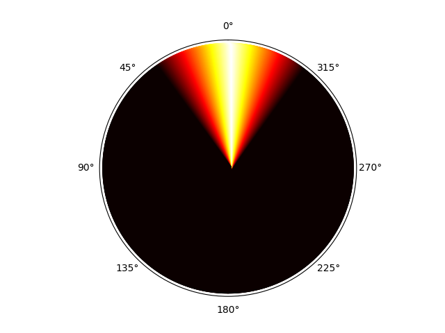
We illustrate our results with some simulations with different initial conditions. We sample $n=2000$ independent uniform point in $\mathbb{T}^{2}$ and we construct the random geometric graph with $\epsilon_{n}=.25$. In Figure 1 we show the results representing the points in $[0,2\pi]^{2}$ and in Figure 2 we show them embedded in $\mathbb{R}^{3}$. In both cases we consider solutions of (1.2) with initial conditions $u_{0}$ as displayed in the leftmost column of both Figure 1 and Figure 2. Observe that all of them represent stable equilibria for the heat equation (1.4). In view of this fact and Theorem 1.2 we expect the solutions of the Kuramoto model (1.2) to remain close to these initial conditions at least in finite time intervals (and arguably for all times). In each figure, each row represents a different initial condition. Different columns represents different moments in time. The first column always represents $t=0$. To improve visualization and to emphasize the twisted states we show $u^{n}(\cdot,t)+t$ instead of $u^{n}(\cdot,t)$ (which corresponds to $\omega=1$ in (1.1)). Figure 3 shows the color representation of each phase $\theta\in\mathbb{S}^{1}$. Videos of these solutions in motion and the code used to generate them can be found in https://github.com/FranCire/TorusKuramoto.

Initial
condition Planar Representation
$u_{0}=x\cdot e_{1}$ [Uncaptioned image] [Uncaptioned image] [Uncaptioned image]
$t=0$ $t=5$ $t=11$
$u_{0}=x\cdot e_{2}$ [Uncaptioned image] [Uncaptioned image] [Uncaptioned image]
$t=0$ $t=2$ $t=11$
$u_{0}=2x\cdot e_{1}$ [Uncaptioned image] [Uncaptioned image] [Uncaptioned image]
$t=0$ $t=5$ $t=14$
$u_{0}=x\cdot(1,1)$ [Uncaptioned image] [Uncaptioned image] [Uncaptioned image]
$t=0$ $t=5$ $t=11$
Figure 1. Planar Representation
Initial
condition 3D Representation
$u_{0}=x\cdot e_{1}$ [Uncaptioned image] [Uncaptioned image] [Uncaptioned image]
$t=0$ $t=5$ $t=11$
$u_{0}=x\cdot e_{2}$ [Uncaptioned image] [Uncaptioned image] [Uncaptioned image]
$t=0$ $t=2$ $t=11$
$u_{0}=2x\cdot e_{1}$ [Uncaptioned image] [Uncaptioned image] [Uncaptioned image]
$t=0$ $t=5$ $t=14$
$u_{0}=x\cdot(1,1)$ [Uncaptioned image] [Uncaptioned image] [Uncaptioned image]
$t=0$ $t=5$ $t=11$
Figure 2. 3D Representation
Refer to caption
Figure 3. Color Palette

Acknowledgments. Pablo Groisman and Hernán Vivas are partially supported by CONICET Grant PIP 2021 11220200102825CO and PICT 2021-00113 from Agencia I+D.

Pablo Groisman is partially supported by UBACyT Grant 20020190100293BA.

Ruojun Huang was supported in part by the Deutsche Forschungsgemeinschaft under Germany’s Excellence Strategy EXC 2044-390685587, Mathematics Münster: dynamics-geometry-structure.

References

  • [1] Pedro Abdalla, Afonso S. Bandeira, and Clara Invernizzi. Guarantees for spontaneous synchronization on random geometric graphs, 2022.
  • [2] J.A. Acebrón, L.L. Bonilla, C.J.P. Vicente, F. Ritort, and R. Spigler. The kuramoto model: A simple paradigm for synchronization phenomena. Reviews of Modern Physics, 77(1):137–185, 2005.
  • [3] Fuensanta Andreu-Vaillo, José M. Mazón, Julio D. Rossi, and J. Julián Toledo-Melero. Nonlocal diffusion problems, volume 165 of Math. Surv. Monogr. Providence, RI: American Mathematical Society (AMS); Madrid: Real Sociedad Matemática Española, 2010.
  • [4] Alex Arenas, Albert Díaz-Guilera, Jurgen Kurths, Yamir Moreno, and Changsong Zhou. Synchronization in complex networks. Phys. Rep., 469(3):93–153, 2008.
  • [5] Rangel Baldasso, Roberto I Oliveira, Alan Pereira, and Guilherme Reis. Large deviations for marked sparse random graphs with applications to interacting diffusions. Preprint, arXiv:2204.08789, 2022.
  • [6] Lorenzo Bertini, Giambattista Giacomin, and Christophe Poquet. Synchronization and random long time dynamics for mean-field plane rotators. Probab. Theory Related Fields, 160(3-4):593–653, 2014.
  • [7] M. Breakspear, S. Heitmann, and A. Daffertshofer. Generative models of cortical oscillations: Neurobiological implications of the kuramoto model. Frontiers in Human Neuroscience, 4, 2010.
  • [8] F. Bullo. Lectures on Network Systems. Kindle Direct Publishing, 1.6 edition, 2022.
  • [9] Hayato Chiba and Georgi S. Medvedev. The mean field analysis of the Kuramoto model on graphs I. The mean field equation and transition point formulas. Discrete Contin. Dyn. Syst., 39(1):131–155, 2019.
  • [10] Fabio Coppini. Long time dynamics for interacting oscillators on graphs. Ann. Appl. Probab., 32(1):360–391, 2022.
  • [11] Fabio Coppini, Helge Dietert, and Giambattista Giacomin. A law of large numbers and large deviations for interacting diffusions on Erdös-Rényi graphs. Stoch. Dyn., 20(2):2050010, 19, 2020.
  • [12] D. Cumin and C. P. Unsworth. Generalising the Kuramoto model for the study of neuronal synchronisation in the brain. Phys. D, 226(2):181–196, 2007.
  • [13] Florian Dörfler and Francesco Bullo. Synchronization in complex networks of phase oscillators: a survey. Automatica J. IFAC, 50(6):1539–1564, 2014.
  • [14] Florian Dörfler, Michael Chertkov, and Francesco Bullo. Synchronization in complex oscillator networks and smart grids. Proc. Natl. Acad. Sci. USA, 110(6):2005–2010, 2013.
  • [15] Lawrence C Evans. Partial differential equations, volume 19. American Mathematical Society, 2022.
  • [16] Pablo Groisman, Ruojun Huang, and Hernán Vivas. The Kuramoto model on dynamic random graphs. Nonlinearity, 36(11):6177–6198, 2023.
  • [17] Martin Kassabov, Steven H. Strogatz, and Alex Townsend. A global synchronization theorem for oscillators on a random graph. Chaos, 32(9):Paper No. 093119, 10, 2022.
  • [18] Y. Kuramoto. Chemical oscillations, waves, and turbulence. volume 19 of Springer Series in Synergetics, pages viii+156. Springer-Verlag, Berlin, 1984.
  • [19] Yoshiki Kuramoto. Self-entrainment of a population of coupled non-linear oscillators. In International Symposium on Mathematical Problems in Theoretical Physics (Kyoto Univ., Kyoto, 1975), pages 420–422. Lecture Notes in Phys., 39, 1975.
  • [20] Shuyang Ling, Ruitu Xu, and Afonso S. Bandeira. On the landscape of synchronization networks: a perspective from nonconvex optimization. SIAM J. Optim., 29(3):1879–1907, 2019.
  • [21] Georgi S. Medvedev. The nonlinear heat equation on dense graphs and graph limits. SIAM J. Math. Anal., 46(4):2743–2766, 2014.
  • [22] Georgi S. Medvedev. The nonlinear heat equation on $W$-random graphs. Arch. Ration. Mech. Anal., 212(3):781–803, 2014.
  • [23] Georgi S. Medvedev. Small-world networks of Kuramoto oscillators. Phys. D, 266:13–22, 2014.
  • [24] Georgi S. Medvedev. The continuum limit of the Kuramoto model on sparse random graphs. Commun. Math. Sci., 17(4):883–898, 2019.
  • [25] Georgi S. Medvedev and Xuezhi Tang. Stability of twisted states in the Kuramoto model on Cayley and random graphs. J. Nonlinear Sci., 25(6):1169–1208, 2015.
  • [26] Georgi S. Medvedev and J. Douglas Wright. Stability of twisted states in the continuum Kuramoto model. SIAM J. Appl. Dyn. Syst., 16(1):188–203, 2017.
  • [27] Renato E. Mirollo and Steven H. Strogatz. Synchronization of pulse-coupled biological oscillators. SIAM J. Appl. Math., 50(6):1645–1662, 1990.
  • [28] Roberto I. Oliveira and Guilherme H. Reis. Interacting diffusions on random graphs with diverging average degrees: hydrodynamics and large deviations. J. Stat. Phys., 176(5):1057–1087, 2019.
  • [29] Roberto I. Oliveira, Guilherme H. Reis, and Lucas M. Stolerman. Interacting diffusions on sparse graphs: hydrodynamics from local weak limits. Electron. J. Probab., 25:35, 2020. Id/No 110.
  • [30] Edward Ott and Thomas M. Antonsen. Low dimensional behavior of large systems of globally coupled oscillators. Chaos, 18(3):037113, 6, 2008.
  • [31] Edward Ott and Thomas M. Antonsen. Long time evolution of phase oscillator systems. Chaos, 19(2):023117, 5, 2009.
  • [32] Charles S Peskin. Mathematical aspects of heart physiology. Courant Inst. Math, 1975.
  • [33] Francisco A. Rodrigues, Thomas K. DM. Peron, Peng Ji, and Jürgen Kurths. The Kuramoto model in complex networks. Phys. Rep., 610:1–98, 2016.
  • [34] Steven Strogatz. Sync: The emerging science of spontaneous order. Penguin UK, 2004.
  • [35] Steven H. Strogatz. From Kuramoto to Crawford: exploring the onset of synchronization in populations of coupled oscillators. Phys. D, 143(1-4):1–20, 2000. Bifurcations, patterns and symmetry.
  • [36] Cecilia De Vita, Julián Fernández Bonder, and Pablo Groisman. The energy landscape of the kuramoto model in one-dimensional random geometric graphs with a hole, 2024.
  • [37] K. Wiesenfeld, P. Colet, and S.H. Strogatz. Synchronization transitions in a disordered josephson series array. Physical Review Letters, 76(3):404–407, 1996.
  • [38] Daniel A. Wiley, Steven H. Strogatz, and Michelle Girvan. The size of the sync basin. Chaos, 16(1):015103, 8, 2006.
  • [39] Arthur T Winfree and Steven H Strogatz. Organizing centres for three-dimensional chemical waves. Nature, 311(5987):611–615, 1984.
  • [40] A.T. Winfree. Biological rhythms and the behavior of populations of coupled oscillators. Journal of Theoretical Biology, 16(1):15–42, 1967.