Curve fitting on a quantum annealer for an advanced navigation method

Abstract

We explore the applicability of quantum annealing to the approximation task of curve fitting. To this end, we consider a function that shall approximate a given set of data points and is written as a finite linear combination of standardized functions, e.g., orthogonal polynomials. Consequently, the decision variables subject to optimization are the coefficients of that expansion. Although this task can be accomplished classically, it can also be formulated as a quadratic unconstrained binary optimization problem, which is suited to be solved with quantum annealing. Given the size of the problem stays below a certain threshold, we find that quantum annealing yields comparable results to the classical solution. Regarding a real-word use case, we discuss the problem to find an optimized speed profile for a vessel using the framework of dynamic programming and outline how the aforementioned approximation task can be put into play.

I Introduction

In 2020, the International Maritime Organization issued a recommendation to navigate just in time such that fuel consumption is minimized while arrival at the destination is guaranteed to be on time [1]. In this case, the approximation corresponds to an optimal speed profile for a vessel along a given trajectory in the sense that fuel consumption is minimized while arrival at the destination is guaranteed to be just in time. The given task is in fact an element of variational calculus and functional analysis. If one discretizes the problem in an attempt to generate a discrete sequence of speed values to support those objectives, one quickly ends up in the domain of dynamic programming and finds the Bellman equation to be a highly valuable tool [2, 3, 4, 5, 6, 7, 8, 9, 10].

Using dynamic programming to address large real-world use cases numerically necessitates a discretization of the problem’s state space. As a consequence, this entails an error in the accuracy of the so-called value function, which is the solution of the Bellman equation, and it is common practice to employ approximation techniques; see, e.g., Refs. [10, 11] and references therein.

One of the most fundamental approximation tasks is curve fitting, where a function is sought that approximates a given set of data, i.e., the difference between the observed data and the approximation shall become minimal. In this work, we formulate the task of curve fitting as a quadratic unconstrained binary optimization (QUBO) problem [12, 13] that is in principle suited to be solved with quantum computing—particularly quantum annealing [14, 15, 16, 17, 18, 19, 20, 21, 22, 23, 24, 25, 26, 27].

Furthermore, in this context we discuss the task of finding an optimized speed profile for a vessel in the sense of minimal fuel consumption while arriving just in time using the framework of dynamic programming. Having the voyage of a vessel in mind, it might very well be the case that finding an optimized speed profile requires a lot of support points in order to densly discretize the state space, especially as soon as the latter becomes high-dimensional, and approximations are practically inevitable. Here, we use the QUBO formulation of curve fitting solved on a quantum annealer to approximate the value function with respect to its dependency on the state space variable.

With quantum computing currently being an emerging technology still in its infancy, we do not expect to outperform a conventional computer. Particularly in view of the fact that the only current commercially available quantum annealing devices manufactured by D-Wave [28, 29, 30, 31, 32, 33, 34, 35, 36, 24, 37] are not full-fledged enough yet, and it is a priori not clear whether their use will result in practical advantages for a specific problem [38, 26, 39, 27].

Nevertheless, in our opinion it is worth to explore to what extent quantum annealing can be applied to real-world use cases that arise in an application- and industry-focused environment (see Ref. [27] for an overview) and to judge the quality of the solutions compared to classical methods. The present work lies within that scope.

The remainder of this article is organized as follows. In Section II, we formulate curve fitting as a QUBO and present our numerical results in Section III. After that, Section IV focuses on finding an optimized speed profile using dynamic programming, and we finally conclude in Section V.

II Curve fitting as a QUBO

Let $X,Y\subset\mathbb{R}$, $n\in\mathbb{N}$, and $\{(x_{i},y_{i})\}_{i=0}^{n-1}\subset X\times Y$ the observed data points. The task is to find an optimal fit function $f^{\ast}\colon X\to Y$ in the sense that the sum of squares of the differences between the observed data $y_{i}$ and approximated values $f^{\ast}(x_{i})$ is minimized (method of least squares) [40]. With $\mathcal{F}$ denoting a suitable function space, we are concerned with the optimization problem

$$\begin{dcases}\min_{f\in\mathcal{F}}Z(f)\,,\\ Z(f)=\sum_{i=0}^{n-1}(y_{i}-f(x_{i}))^{2}\,.\end{dcases}$$ (1)

With this problem definition, the best fit is thus given by $f^{\ast}=\operatorname*{arg\,min}_{f\in\mathcal{F}}Z(f)$. For example, if $f(x)=a_{0}+a_{1}x$ with optimization parameters $a_{0},a_{1}\in\mathbb{R}$, the minimization task 1 corresponds to simple linear regression.

Here, we allow for a more general expression for $f$ and express it as a finite linear combination of standardized functions $\{\phi_{j}\colon X\to Y\}_{j=0}^{m-1}\subset\mathcal{F}$, $m\in\mathbb{N}$, i.e.,

$$f(x)=\sum_{j=0}^{m-1}c_{j}\phi_{j}(x)\,.$$ (2)

For example, such expansions are frequently employed within a certain area of high-energy physics where they aid to handle the numerical complexity of the occurring equations [41, 42]. Two customary choices for $\phi_{j}$ are:

• orthogonal polynomials such as Chebyshev polynomials. The first kind of the latter, $T_{j}$, are defined via the recurrence relation

  $$T_{j}(x)=2xT_{j-1}(x)-T_{j-2}(x)$$ (3)

  for $j\geq 2$ with $T_{1}(x)=x$ and $T_{0}(x)=1$ [43];

• triangular functions $\Lambda_{j}$ that yield a piecewise-linear approximation. They are defined with respect to supporting points $\tilde{x}_{0}<\dotso<\tilde{x}_{m-1}$, $m>2$, with $\tilde{x}_{0}=x_{0}$ and $\tilde{x}_{m-1}=x_{n-1}$ according to

  $$\Lambda_{j}(x)=\begin{dcases}\frac{x-\tilde{x}_{j-1}}{\tilde{x}_{j}-\tilde{x}_{j-1}}&\text{if\leavevmode\nobreak\ }x\in[\tilde{x}_{j-1},\tilde{x}_{j})\,,\\[2.5pt] \frac{\tilde{x}_{j+1}-x}{\tilde{x}_{j+1}-\tilde{x}_{j}}&\text{if\leavevmode\nobreak\ }x\in[\tilde{x}_{j},\tilde{x}_{j+1})\,,\\[2.5pt] 0&\text{otherwise}\,,\end{dcases}$$ (4)

  where it is understood that only the first (second) branch defines the nonzero values of the last (first) triangular function $\Lambda_{j=m-1}$ ($\Lambda_{j=0}$).

II.1 Classical solution

We aim to determine the expansion coefficients $c_{j}$ in Eq. 2 according to the least-squares principle as given by the optimization problem 1. With the abbreviations (where $j,k=0,\dotsc,m-1$)

$$b_{j} =\sum_{i=0}^{n-1}y_{i}\phi_{j}(x_{i})\,,$$ (5)

$$W_{jk} =\sum_{i=0}^{n-1}\phi_{j}(x_{i})\phi_{k}(x_{i})\,,$$ (6)

vectors $c=[c_{0},\dotsc,c_{m-1}]^{\top}\in\mathbb{R}^{m}$, $b=[b_{0},\dotsc,b_{m-1}]^{\top}\in\mathbb{R}^{m}$, and the symmetric matrix $W\in\mathbb{R}^{m\times m}$ with entries $W_{jk}$, the optimization problem upon inserting Eq. 2 into 1 now reads

$$\begin{dcases}\min_{c\in\mathbb{R}^{m}}Z(c)\,,\\ Z(c)=c^{\top}Wc-2c^{\top}b\,.\end{dcases}$$ (7)

The optimal weight coefficients $c^{\ast}$ thus follow from

$$\nabla Z(c^{\ast})=2\,(Wc^{\ast}-b)\stackrel{{\scriptstyle!}}{{=}}0$$ (8)

and are explicitly given by

$$c^{\ast}=W^{-1}b$$ (9)

provided $W$ is invertible. If this is not the case, in practice one could resort to its Moore–Penrose pseudoinverse [44].

II.2 Quantum annealing-oriented approach

Starting from the objective function as given in 7 in its expanded form

$$Z(c)=\sum_{j=0}^{m-1}\sum_{k=0}^{m-1}c_{j}W_{jk}c_{k}-2\sum_{j=0}^{m-1}c_{j}b_{j}\,,$$ (10)

we have a quadratic function in the components of $c$. With each component of the latter being a real number, it can be written as a difference of two positive real numbers, i.e., $c_{j}=c_{j}^{+}-c_{j}^{-}$ with $c_{j}^{\pm}\in\mathbb{R}_{\geq 0}$. Now, in order to express the optimization problem 7 as a QUBO, whose decision variables’ domain is the binary set $\{0,1\}$, we decompose $c_{j}^{\pm}$ into powers of two, i.e., write them in binary form. This yields the following expression for the expansion coefficients:

$$c_{j}=\sum_{r=0}^{L+U}2^{r-L}\hskip 0.83344pt\bigl{(}\psi_{jr}^{+}-\psi_{jr}^{-}\bigr{)}\,,$$ (11)

where $L,U\in\mathbb{N}$ are appropriate lower and upper bounds for the binary representation of the expansion coefficients, respectively. $L$ defines the precision with which the decimal places of a real number are represented in a binary expansion. The coefficients $\psi_{jr}^{\pm}\in\{0,1\}$ are then the new decision variables represented by the qubits states of a quantum annealing device.

Here, we tacitly assume that there exists a precision goal that is suitable for all $c_{j}$. In other words, though $L$ and $U$ are (most likely) different for different sets of the underlying to-be-approximated data, they are assumed to be independent of $j$.

Inserting Eq. 11 into 10 yields an objective function depending on $\psi^{\pm}=[\psi_{00}^{\pm},\psi_{01}^{\pm},\dotsc]^{\top}\in\{0,1\}^{m(L+U+1)}$, i.e., on all coefficients of the binary representation of the expansion coefficients; to wit

$$Z(\psi^{\pm}) =\sum_{j=0}^{m-1}\sum_{k=0}^{m-1}\sum_{r=0}^{L+U}\sum_{s=0}^{L+U}2^{r+s-2L}W_{jk}$$

$$\phantom{=\;}\times\bigl{(}\psi_{jr}^{+}\psi_{ks}^{+}+\psi_{jr}^{-}\psi_{ks}^{-}-\psi_{jr}^{+}\psi_{ks}^{-}-\psi_{jr}^{-}\psi_{ks}^{+}\bigr{)}$$

$$\phantom{=\;}-\sum_{j=0}^{m-1}\sum_{r=0}^{L+U}2^{r-L+1}b_{j}\hskip 0.83344pt\bigl{(}\psi_{jr}^{+}-\psi_{jr}^{-}\bigr{)}\,.$$ (12)

With $d=L+U+1$, this equation can be written as

$$Z(\psi^{\pm}) =\sum_{p=0}^{md-1}\sum_{q=0}^{md-1}\bigl{(}\psi_{p}^{+}\psi_{q}^{+}+\psi_{p}^{-}\psi_{q}^{-}$$

$$\phantom{=\;}-\psi_{p}^{+}\psi_{q}^{-}-\psi_{p}^{-}\psi_{q}^{+}\bigr{)}\hskip 0.83344ptW_{pq}^{\prime}$$

$$\phantom{=\;}-\sum_{p=0}^{md-1}\bigl{(}\psi_{p}^{+}-\psi_{p}^{-}\bigr{)}\hskip 0.83344ptb_{p}^{\prime}\,,$$ (13)

where $\psi_{p}^{\pm}=\psi_{\hat{p}\tilde{p}}^{\pm}$, $b_{p}^{\prime}=2^{\tilde{p}-L+1}b_{\hat{p}}$, and $W_{pq}^{\prime}=2^{\tilde{p}+\tilde{q}-2L}W_{\hat{p}\hat{q}}$ with $\hat{p}=\lfloor\hskip 0.83344ptp/d\rfloor$ and $\tilde{p}=p\bmod d$ (analogously for $q$). $b_{p}^{\prime}$ and $W_{pq}^{\prime}$ are the entries of the quantities $b^{\prime}\in\mathbb{R}^{md}$ and $W^{\prime}\in\mathbb{R}^{(md)\times(md)}$, respectively.

Now, in order to cast the objective function 13 into the canonical QUBO form, we introduce the quantities (using block-matrix notation)

$$\psi =\biggl{[}\hskip 0.83344pt\begin{matrix}\psi^{+}\\[2.5pt] \psi^{-}\end{matrix}\hskip 0.83344pt\biggr{]}\in\{0,1\}^{2md}\,,$$ (14)

$$b^{\prime\prime} =\biggl{[}\hskip 0.83344pt\begin{matrix}b^{\prime}\\[2.5pt] -b^{\prime}\end{matrix}\hskip 0.83344pt\biggr{]}\in\mathbb{R}^{2md}\,,$$ (15)

$$W^{\prime\prime} =\biggl{[}\hskip 0.83344pt\begin{matrix}W^{\prime}&-2\hskip 0.83344ptW^{\prime}\hskip 0.83344pt\\[2.5pt] 0&W^{\prime}\end{matrix}\hskip 0.83344pt\biggr{]}\in\mathbb{R}^{(2md)\times(2md)}\,,$$ (16)

which allows us to write the objective function in a rather compact form:

$$Z(\psi)=\psi^{\top}W^{\prime\prime}\psi-\psi^{\top}b^{\prime\prime}\,.$$ (17)

Furthermore, since $\psi$ is a binary vector, its entries are idempotent, $(\psi_{p}^{\pm})^{2}=\psi_{p}^{\pm}$ for all $p$, and the linear term in Eq. 17 can be written as a contribution that is subtracted from the diagonal elements of $W^{\prime\prime}$. Thus, our final expression for the least-squares optimization problem 1 written as a QUBO reads

$$\begin{dcases}\min_{\psi\in\{0,1\}^{2md}}Z(\psi)\,,\\ Z(\psi)=\psi^{\top}Q\hskip 0.83344pt\psi\end{dcases}$$ (18)

with $Q=W^{\prime\prime}-\operatorname{diag}(b_{0}^{\prime\prime},b_{1}^{\prime\prime},\dotsc)\in\mathbb{R}^{(2md)\times(2md)}$. Apparently, the number of required qubits depends only on the number of standardized functions $m$ and the precision of the binary decomposition of the expansion coefficients characterized by $L$ and $U$.

III Numerical results

In the following, we present and discuss our numerical results of the curve fitting task by means of a QUBO problem as described above.

Since we shall compare results obtained on a classical computer using a tabu search [45, 46, 47] with results from a D-Wave quantum annealing device, we briefly sketch how the latter works (see, e.g., Refs. [36, 24, 37, 48] and references therein for more details). In very short: inspired by adiabatic quantum computing [25], quantum annealing as implemented by D-Wave is a heuristic method to find the ground state of an Ising spin model [49, 50]. For a system of spins $s=(s_{0},\dotsc,s_{N-1})\in\{-1,1\}^{N}$, $N\in\mathbb{N}$, the ground state is a spin configuration that globally minimizes the objective function

$$Z_{\textup{Ising}}(s)=\sum_{i=0}^{N-1}\sum_{j=i+1}^{N-1}J_{ij}s_{i}s_{j}+\sum_{i=0}^{N-1}h_{i}s_{i}\,,$$ (19)

where $J_{ij}$ and $h_{i}$ denote the nearest-neighbor interaction between the $i\hskip 0.83344pt$^th and $j\hskip 0.83344pt$^th spin (coupling strength) and an external magnetic field acting on the $i\hskip 0.83344pt$^th spin (qubit bias), respectively.

The connection to the corresponding QUBO model with objective function $Z_{\textup{QUBO}}(z)=z^{\top}R\hskip 0.83344ptz$ with $z\in\{0,1\}^{N}$ and an upper-triangular matrix $R\in\mathbb{R}^{N\times N}$ is established by $s_{i}=2z_{i}-1$. The off- and on-diagonal entries of $R$ are mapped onto the coupling strengths and qubit biases, respectively. It is straightforward to show that the Ising and QUBO objective functions differ only by an additive constant, $Z_{\textup{Ising}}(s)=Z_{\textup{QUBO}}(z)+\textup{const.}$, i.e., the solution of a given QUBO problem can be equivalently obtained by finding a ground state of an Ising model.

III.1 Linear regression

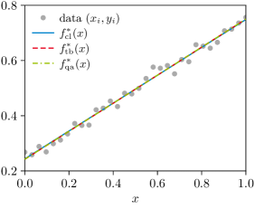
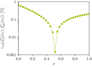
Figure 1: Left: data (gray dots) together with optimal regression lines obtained classically ($f_{\textup{cl}}^{\ast}$, solid blue) and by a QUBO solved with tabu search ($f_{\textup{tb}}^{\ast}$, dashed red) as well as quantum annealing ($f_{\textup{qa}}^{\ast}$, dash-dotted green). Right: relative error between the classical and quantum annealing solution.

We proceed with our numerical investigations and begin with the simple yet important case of linear regression. To this end, we choose $n=32$ and consider the mock data ($i=0,\dotsc,n-1$)

$$x_{i}=\frac{i}{n-1}\,,\qquad y_{i}=\frac{1}{2}x_{i}+\frac{1}{4}+\textup{noise}\,,$$ (20)

where the ordinate values are distorted by artificial noise. At each $y_{i}$, it is a sample drawn from a normal distribution centered about zero with a standard deviation of $0.02$.

Regarding the expansion $f(x)=\sum_{j=0}^{m-1}c_{j}\phi_{j}(x)$ of the fit function, linear regression corresponds to $m=2$ and $\phi_{0}(x)=1$, $\phi_{1}(x)=x$ such that $f(x)=c_{0}+c_{1}x$ with regression parameters $c_{0}$ and $c_{1}$. For the corresponding QUBO problem, we choose $L=7$ and $U=1$, which is sufficient for the expected order of magnitude of the regression parameters. Since the latter are expected to be positive, the general QUBO problem of size $(2md)\times(2md)$ can be reduced to $(md)\times(md)$, yielding a matrix of size $18\times 18$ for this problem.

In the left diagram of Fig. 1, we show the data as given in Eq. 20 (gray dots) together with the optimal regression lines $f^{\ast}(x)=c_{0}^{\ast}+c_{1}^{\ast}x$ with optimal coefficients $c_{0}^{\ast}$ and $c_{1}^{\ast}$ obtained classically (solid blue), i.e., according to Section II.1 (specifically, using Eq. 9), and by solving the corresponding QUBO formulation via tabu search on a conventional computer (dashed red) as well as through quantum annealing on a D-Wave device (dash-dotted green). Comparing the three solutions, we find that the results for the regression lines agree up to the second decimal point. Moreover, the solution obtained via tabu search is also found by quantum annealing, their results are identical. In order to gauge the quality of the quantum annealing solution, in the right diagram of Fig. 1 we show the relative error

$$\varepsilon_{\textup{rel}}(a,b)=\frac{\lvert a-b\rvert}{\max\{\lvert a\rvert,\delta\}}\qquad(a,b\in\mathbb{R},\,\delta>0)$$ (21)

between the regression lines obtained classically and through quantum annealing. It is below one percent for all abscissae of the data. For the sake of completeness, in Tab. 1 we show the results for the optimal regression parameters.

Thus, in the case of linear regression, our results show that formulating curve fitting as a QUBO problem indeed works and yields a solution on-par with the classical one. They also suggest that quantum annealing in its current state is (within limits) able to deliver promising and practically usable results for this continuous problem.

	$c_{0}^{\ast}$	$c_{1}^{\ast}$
Classical solution	$0.24377$	$0.50474$
Quantum annealing	$0.24219$	$0.50781$
$\varepsilon_{\textup{rel}}$ [%]	$0.65$	$0.61$

Table 1: Optimal regression parameters obtained classically and via quantum annealing.

III.2 Piecewise-linear approximation

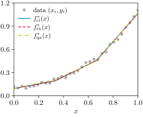
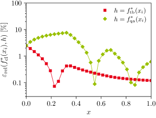
Figure 2: Left: data (gray dots) together with optimal piecewise-linear approximations obtained classically ($f_{\textup{cl}}^{\ast}$, solid blue) and by a QUBO solved with tabu search ($f_{\textup{tb}}^{\ast}$, dashed red) as well as quantum annealing ($f_{\textup{qa}}^{\ast}$, dash-dotted green). Right: relative errors between the classical solution and the tabu search as well as quantum annealing solutions.

We continue with an example where linear regression is not appropriate. Inspired by observations we have made during the analysis of fuel-consumption data of a container vessel, we now consider the data

$$x_{i}=\frac{i}{n-1}\,,\qquad y_{i}=\frac{1}{4}x_{i}+\frac{3}{4}x_{i}^{3}+\frac{1}{10}+\textup{noise}\,,$$ (22)

again with $n=32$, and the noise are samples drawn from a normal distribution. These data points shall be approximated by a piecewise linear function. To this end, we choose $m=4$ and use triangular functions for the function expansion, $\phi_{j}=\Lambda_{j}$ (see Eq. 4); their supporting points $\tilde{x}_{0},\dotsc,\tilde{x}_{3}$ are linearly distributed over the abscissa interval $[0,1]$. For the QUBO problem, we choose $L=8$ and $U=1$.

In the left diagram of Fig. 2, we display the optimal fit $f^{\ast}(x)=c_{0}^{\ast}\Lambda_{0}(x)+\dotso+c_{3}^{\ast}\Lambda_{3}(x)$ obtained classically according to Eq. 9 (solid blue) and by solving the QUBO via tabu search (dashed red) as well as quantum annealing (dash-dotted green). Compared to linear regression, the tabu solution is again not distinguishable from the classical one by the eye while the quantum annealing solution shows slight deviations. However, the latter are rather small, and although the QUBO matrix is more than twice as large ($40\times 40$) as for linear regression, the overall fit quality of the quantum solution is still satisfying. This is also reflected in the relative errors between the classical and QUBO solutions that are below ten percent across the whole abscissa range (right diagram of Fig. 2). In Tab. 2, we show the results for the optimal coefficients.

	$c_{0}^{\ast}$	$c_{1}^{\ast}$	$c_{2}^{\ast}$	$c_{3}^{\ast}$
Classical	$0.09149$	$0.19231$	$0.45782$	$1.06377$
Quantum	$0.09375$	$0.20703$	$0.44922$	$1.07031$
$\varepsilon_{\textup{rel}}$ [%]	$2.47$	$7.65$	$1.88$	$0.61$

Table 2: Optimal coefficients of the individual triangular functions obtained classically and via quantum annealing.

III.3 Chebyshev polynomials

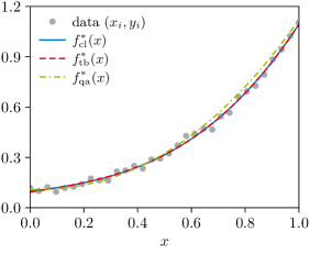
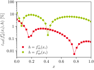
Figure 3: Left: data (gray dots) together with optimal Chebyshev approximations obtained classically ($f_{\textup{cl}}^{\ast}$, solid blue) and by a QUBO solved with tabu search ($f_{\textup{tb}}^{\ast}$, dashed red) as well as quantum annealing ($f_{\textup{qa}}^{\ast}$, dash-dotted green). Right: relative errors between the classical solution and the tabu search as well as quantum annealing solutions.

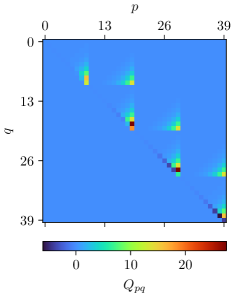
Figure 4: Heat map plots of the QUBO matrices $Q$ of the piecewise-linear approximation (left) and Chebyshev polynomial approximation (right) as discussed in Sections III.2 and III.3, respectively. Here, we display the upper-triangularized versions of these matrices since every QUBO problem can be written in a way such that $Q$ is an upper-triangular matrix.

Last, we use Chebyshev polynomials of the first kind for fitting the data described in Eq. 21, $\phi_{j}=T_{j}$ (see Eq. 3), again with $m=4$. Thus, the fit function reads explicitly

$$f(x)=c_{0}+c_{1}x+c_{2}\hskip 0.83344pt(2x^{2}-1)+c_{3}\hskip 0.83344pt(4x^{3}-3x)\,.$$ (23)

For the corresponding QUBO formulation, we use the same precision as before ($L=8$ and $U=1$).

As apparent from the results shown in Fig. 3, the tabu solution of the QUBO problem is again practically identical to the classical one. On the other hand, the quantum solution now shows visible deviations in form of under- and overshooting with respect to the tabu and classical solutions. The corresponding relative error is about ten percent while the one for the tabu solution is roughly one magnitude smaller.

Thus, even though the QUBO matrix is of the same size as for the piecewise-linear approximation and constructed from the same underlying set of data points, the resulting quantum annealing solution for the Chebyshev approximation is of lower quality than the one for a piecewise-linear curve fitting using triangular functions. We find that this is also the case if we change the precision of the binary decomposition of the expansion coefficients (see Eq. 11) by varying $L$ and/or $U$, i.e., for smaller or larger QUBO matrices, and we were not able to find a quantum annealing solution with the same quality as the ones for linear regression and piecewise-linear approximation. From our point of view though, the quantum result shown in Fig. 3 is still reasonable.

Alas, for a QUBO matrix with a size of about $60\times 60$ and larger, we were not able to find a satisfying solution for the Chebyshev approximation through quantum annealing at all, while a high-quality solution can still be found via tabu search. For the said size of the QUBO problem, finding a satisfying piecewise-linear approximation solely using quantum annealing (i.e., with a relative error of about ten percent compared to the tabu solution) is also rather difficult. From our point of view, this seems to hint toward the limitations of the current quantum annealing hardware for this problem.

More precisely, the QUBO problem, which can be seen as a graph with logical qubits representing nodes that are connected by edges with weights given by the matrix elements of the QUBO matrix, needs to be mapped onto the so-called working graph of the quantum annealing device. Therefore, one might need several physical qubits to represent one logical qubit. Particularly for large and densly-connected QUBO problems, this could yield an Ising model that exhibits a complicated low-energy landscape where the ground state is difficult to access. This would explain why we were not successful in obtaining a feasible Chebyshev approximation as soon as its QUBO matrix is larger than the above mentioned size of about $60\times 60$ because the matrix is, as apparent from the right diagram of Fig. 4, indeed relatively highly connected.

The amount of nonvanishing off-diagonal elements of the QUBO matrix for least-squares curve fitting is solely determined by the standardized functions $\phi_{j}$ (keeping the underlying to-be-approximated data fixed); see Eq. 6. More precisely, in case of the Chebyshev approximation we deal with polynomials $T_{j}$ whose support are the whole real line,

$$\operatorname{supp}(T_{j})=\mathbb{R}$$ (24)

for all $j$. Therefore, the resulting QUBO problem corresponds to a rather highly connected graph, and the matrix has many nonzero elements even far off the diagonal; see the right diagram of Fig. 4 for a graphical depiction. On the other hand, the QUBO matrix for a piecewise-linear approximation is always a band matrix, see the left diagram of Fig. 4, because the triangular functions $\Lambda_{j}$ have compact support,

$$\operatorname{supp}(\Lambda_{j})=\begin{cases}[\tilde{x}_{0},\tilde{x}_{1}]&\text{if\leavevmode\nobreak\ }j=0\,,\\[2.5pt] [\tilde{x}_{m-2},\tilde{x}_{m-1}]&\text{if\leavevmode\nobreak\ }j=m-1\,,\\[2.5pt] [\tilde{x}_{j-1},\tilde{x}_{j+1}]&\text{otherwise}\,.\end{cases}$$ (25)

In our opinion, this explains why

• we are unsuccessful in finding a satisfying quantum annealing solution for the Chebyshev approximation for QUBO matrices larger than a certain size;

• the Chebyshev solution is less accurate compared to the piecewise-linear approximation for feasible cases of the size of the QUBO problem.

Furthermore, another obstacle might be the order of magnitude of the elements of the QUBO matrix. These have to be mapped onto the coupling strengths and qubit biases of the Ising model, which are constrained by the physical limits of the quantum annealing hardware, i.e., the available ranges of couplings and biases as well as their coarseness. As a consequence, it might be the case that a complicated low-energy landscape cannot be “scanned” accurate enough by the current quantum annealing devices. Unfortunately, the actual values of these matrix elements are determined by the to-be-approximated data and the employed standardized functions $\phi_{j}$ and thus cannot be freely adjusted or altered.

Finally, we would like to emphasize that by solving the QUBO problems for piecewise-linear and Chebyshev approximations using a heuristic technique, e.g., tabu search or simulated annealing, we (almost) always find a solution practically on-par with the classical one—even for sizes of the QUBO matrix for which the quantum annealing solution turned out to be unpractical. Thus, we are confident that a next-generation quantum annealing device will be capable of solving these larger QUBO problems in the future.

IV Speed profile optimization with dynamic programming

In this section, we touch upon a real-world use case, with which we are currently concerned, where curve fitting can come in handy. Namely, a cargo vessel’s voyage under the constraint of minimal fuel consumption while arriving at the destination at the requested time of arrival. Phrased differently, the aim is to find an optimized speed profile that minimizes fuel costs while arriving just in time. From our point of view, this task lends itself to be solved within the framework of dynamic programming [2, 3, 4]; see, e.g., Refs. [5, 6, 7, 8, 9, 10] for comprehensive overviews. Work in that direction has been done regarding the optimal control of sailboats [51, 52, 53]. To our knowledge, however, dynamic programming is not used for maritime just-in-time navigation of cargo vessels yet, and we would like to leverage its use.

IV.1 General formalism

More formally speaking, we consider a deterministic Markov decision process that starts at time $t=0$ and terminates at $t=T$, where the time evolution is discrete in terms of integer time steps: $t=0,\dotsc,T$. The process is characterized by sets $X_{t}\subset\mathbb{R}^{k}$ and $U_{t}\subset\mathbb{R}^{l}$, where $k,l\in\mathbb{N}$, that contain all states the process can be in and all actions that can be performed in order to change the current state, respectively, at time step $t$.

The dynamics of the decision process, i.e., how the next state $x_{t+1}\in X_{t+1}$ is obtained from the previous one $x_{t}\in X_{t}$ by performing a certain action $u_{t}\in U_{t}$, are governed by a transition function $\Gamma_{t}\colon X_{t}\times U_{t}\to X_{t+1}$; that is,

$$x_{t+1}=\Gamma_{t}(x_{t},u_{t})\,.$$ (26)

The immediate costs that occur if the action $u_{t}$ is performed while being in state $x_{t}$ are given by a cost function $C_{t}\colon X_{t}\times U_{t}\to\mathbb{R}$. This motivates the definition of a value function $V_{t}\colon X_{t}\times U_{t}\times\dotso\times U_{T-1}\to\mathbb{R}$, which is given by

$$V_{t}(x_{t},u_{t},\dotsc,u_{T-1})=\sum_{s=t}^{T-1}C_{s}(x_{s},u_{s})+D(x_{T})\,,$$ (27)

where $D\colon X_{T}\to\mathbb{R}$ encodes terminal costs that occur at the end of the process. The value function is a measure for how cost-effectively the decision process has been if started at time step $t$ with initial state $x_{t}$ and running until the end by virtue of a given sequence of actions $u_{t},\dotsc,u_{T-1}$. The states $x_{t+1},\dotsc,x_{T}$ in Eq. 27 are generated according to the temporal evolution defined by the process’ dynamics 26.

The goal is to find optimal actions $u_{t}^{\ast},\dotsc,u_{T-1}^{\ast}$ that minimize the cost function for a given initial state. Consequently, these optimal actions, which can be regarded as a recipe how to operate the process such that minimal total costs incur, are encoded in the optimal value function $V_{t}^{\ast}\colon X_{t}\to\mathbb{R}$, which reads

$$V_{t}^{\ast}(x_{t})=\min_{\begin{subarray}{c}u_{s}\in U_{s}\\ s=t,\dotsc,T-1\end{subarray}}V_{t}(x_{t},u_{t},\dotsc,u_{T-1})\,.$$ (28)

For any given initial state, it yields the optimal remaining costs; usually, one is interested in $V_{0}^{\ast}$, i.e., the total optimal costs for the whole process. Now, it can be shown that $V_{t}^{\ast}$ obeys the so-called Bellman equation [2, 3, 4, 5], which lies at the heart of the dynamic programming paradigm and plays an important role in the field of reinforcement learning [9, 10]. It relates the optimal value function at different time steps in a recursive manner and is given by

$$V_{t}^{\ast}(x_{t})=\min_{u_{t}\in U_{t}}\bigl{\{}C_{t}(x_{t},u_{t})+V_{t+1}^{\ast}(x_{t+1})\bigr{\}}$$ (29)

for $t=0,\dotsc,T-1$ and all $x_{t}\in X_{t}$ with $x_{t+1}=\Gamma_{t}(x_{t},u_{t})$ and boundary condition $V_{T}^{\ast}(x_{T})=D(x_{T})$.

Solving the recursively-coupled set of equations is a nontrivial task. Fortunately, the Bellman equation suggests a practical algorithm to obtain the globally optimal solution. Typically, one is interested in the optimal control $u_{0}^{\ast},\dotsc,u_{T-1}^{\ast}$ of the whole process. The solution strategy consists of a backward (value) and forward (policy) iteration; see, e.g., Ref. [6]. First, one computes the function values of the optimal value function starting from the last time step and then moving sequentially backward in time, i.e., for all $t=T,\dotsc,0$ and for all states $x_{t}\in X_{t}$, the values $V_{t}^{\ast}(x_{t})$ are computed according to Eq. 29. Second, the optimal actions are obtained via

$$u_{t}^{\ast}=\operatorname*{arg\,min}_{u_{t}\in U_{t}}\bigl{\{}C_{t}(x_{t}^{\ast},u_{t})+V_{t+1}^{\ast}(\Gamma_{t}(x_{t}^{\ast},u_{t}))\bigr{\}}$$ (30)

with $x_{t+1}^{\ast}=\Gamma_{t}(x_{t}^{\ast},u_{t}^{\ast})$ and initial state $x_{0}=x_{0}^{\ast}$ for $t=0,\dotsc,T-1$, i.e., forward in time.

IV.2 Toward an optimized speed profile

In principle, the Bellman equation as given in Eq. 29 can be used right away to compute an optimized speed profile. The mapping onto that task is, for example, accomplished by the following setup:

• the trajectory of the vessel is fixed and covers a certain distance of $\ell$ nautical miles;

• $X_{t}$ contains all feasible positions of the vessel on the trajectory (i.e., the distances traveled since departure at time $t=0$) and environmental aspects like weather, currents, and forecasts at time $t$;

• $U_{t}$ contains all feasible speeds (through water) of the vessel at time $t$;

• $C_{t}(x_{t},u_{t})$ are the fuel costs that arise if the vessel moves with speed $u_{t}$ while being at position $x_{t}$ at time $t$;

• $\Gamma_{t}(x_{t},u_{t})$ describes how a speed of $u_{t}$ while being at position $x_{t}$ at time $t$ translates into a change in position to $x_{t+1}$.

Given that all of the above are available, particularly the cost and transition functions for arbitrary $x_{t}$ and $u_{t}$, solving the Bellman equation yields optimal speeds and positions $u_{0}^{\ast},\dotsc,u_{T-1}^{\ast}$ and $x_{0}^{\ast},\dotsc,x_{T}^{\ast}$, respectively, on the trajectory that globally minimize the value function, i.e., provide the optimal operating scenario for just-in-time arrival at minimal fuel consumption.

IV.3 Proof of principle

As a proof of principle, in the following we investigate a simple implementation of what we described above in the previous subsection. We set

$$X_{t},U_{t} \subset\mathbb{R}\,,$$ (31)

$$C_{t}(x_{t},u_{t}) =\biggl{(}\frac{u_{t}-w(x_{t})}{v_{\textup{max}}}\biggr{)}^{2}\,,$$ (32)

$$x_{t+1} =\Gamma_{t}(x_{t},u_{t})=x_{t}+u_{t}-w(x_{t})\,,$$ (33)

$$D(x_{T}) =\alpha\,\Bigl{(}1-\frac{x_{T}}{\ell}\Bigr{)}^{2}+1$$ (34)

for all $t$. Here, $w\colon X_{t}\to\mathbb{R}$ denotes the magnitude of the projected sea current with respect to the direction of travel at position $x_{t}$ on the trajectory, $v_{\textup{max}}$ represents the maximal possible speed through water, and $\alpha\in\mathbb{R}_{>0}$ is a numerical parameter to fine-tune the terminal costs.

Upon inserting these definitions into Eq. 27 and writing the final state as $x_{T}=x_{0}+\sum_{t=0}^{T-1}(u_{t}-w(x_{t}))$, which follows directly from Eq. 33, the value function for the whole process reads

$$V_{0}(x_{0},u_{0},\dotsc,u_{T-1}) =\frac{1}{v_{\textup{max}}^{2}}\sum_{t=0}^{T-1}(u_{t}-w(x_{t}))^{2}$$

$$\phantom{=\;}+\frac{\alpha}{\ell}\biggl{[}\ell-x_{0}-\sum_{t=0}^{T-1}(u_{t}-w(x_{t}))\biggr{]}^{2}$$

$$\phantom{=\;}+1\,.$$ (35)

Without loss of generality (and for numerical convenience), we assume that the sets of states and actions $X_{t}$ and $U_{t}$, respectively, are the same for every time step, i.e., independent of $t$. It is then straightforward to find the optimal actions, which are the roots of $\nabla_{u}V_{0}$ (for fixed $x_{0}$). Regarding the gradient of the value function, we find

$$\frac{\partial V_{0}}{\partial u_{t}} =\frac{2u_{t}}{v_{\textup{max}}^{2}}-\frac{2\alpha}{\ell^{2}}\biggl{[}\ell-x_{0}-\sum_{s=0}^{T-1}(u_{s}-w(x_{s}))\biggr{]}\,.$$ (36)

Now, we shall solve this optimization problem by numerically solving the Bellman equation 29 and subsequently using Eq. 30 to find the optimal actions. For the sake of simplicity, we set $w(x_{t})=0$ for all $x_{t}\in X_{t}$ and all $t$, and consider a voyage with $\ell=100$, $v_{\textup{max}}=50$, and $T=4$. Neglecting phases of (de)acceleration and without currents, the optimal solution is obviously $u_{0}^{\ast}=\dotso=u_{3}^{\ast}=25$, i.e., moving (trivially) with constant velocity. Approaching this problem in terms of the value function 34, we find from $\nabla_{u}V_{0}=0$ (see Eq. 36) the analytical solution

$$u_{t}^{\ast}=\frac{\ell}{T+\ell^{2}/(\alpha v_{\textup{max}}^{2})}$$ (37)

for all $t=0,\dotsc,3$. As expected, this analytical solution describes a constant time-independent velocity, which consistently coincides with the optimal solution in the limit $\alpha\to\infty$, i.e., for infinite terminal costs. This analytical solution (with finite $\alpha$) shall serve for comparison with results from solving the Bellman equation numerically.

In the course of that, the traditional/naive approach discretizes the state space. Hence, after the value iteration, the resulting optimal value function $V_{t}^{\ast}$ is defined only on that discrete state space grid. Consequently, this poses constraints on the possible discretizations of the action space for the policy iteration 30 because for a given $x_{t}$, $u_{t}$ must be chosen such that $x_{t+1}=\Gamma_{t}(x_{t},u_{t})$ lies on the state space grid, too, or the off-grid result $\Gamma_{t}(x_{t},u_{t})$ has to be “snapped” onto the nearest grid point. Both approaches induce a discretization error that manifests in the final (pseudo-)optimal policy. The in that way obtained optimal policy most likely differs from the true, globally-optimal solution—it is only optimal with respect to the discretization of the state space. In our case, this would result in a pseudo-optimal speed profile different from the analyical solution 37.

In principle, this issue can be mitigated by using a sufficiently dense state space grid. In our opinion, however, this is not feasible for many real-world use cases due to limitations in CPU hours and/or memory. At this point, curve fitting comes in handy. Following Ref. [10], we approximate the optimal value function in the Bellman equation for each time step separately by a linear combination of standardized functions. This is a promising approach because the optimal value function is expected to be continuous in the state variable. More precisely, for each $t$ we write

$$\hat{V}_{t}^{\ast}(x_{t})=\sum_{j=0}^{m-1}c_{j}^{(t)}\phi_{j}(x_{t})$$ (38)

with $m\in\mathbb{N}$, and $\phi_{j}\colon X_{t}\to\mathbb{R}$ denote suitable standardized (basis) functions. Here, we used the circumflex notation to indicate that the optimal value function is approximated, and the superscript of the expansion coefficients emphasizes that there is a separate approximation for each time step.

The value iteration takes the same form as before (see Section IV.1) but with the subtle yet important difference, that the optimal value function is approximated at every time step. Starting from the end of the horizon and moving backward in time, the approximation at time step $t$ is then used for $t-1$. We start at the finite horizon with the boundary condition $\hat{V}_{T}^{\ast}(x_{T})=D(x_{T})$ and then proceed backward with

$$\hat{V}_{t}^{\ast}(x_{t})=\min_{u_{t}\in U_{t}}\bigl{\{}C_{t}(x_{t},u_{t})+\hat{V}_{t+1}^{\ast}(x_{t+1})\bigr{\}}$$ (39)

for $t=T-1,\dotsc,0$. Here, it is worth to empasize that at every time step, this value iteration uses only a subset of the state space due to the involved approximation, which allows for an efficient treatment of large state spaces. In the literature, this idea is also known as fitted value iteration [10]. Eventually, the resulting sequence $\hat{V}_{T}^{\ast},\dotsc,\hat{V}_{0}^{\ast}$ of optimal approximated value functions is used in the usual policy iteration 30. Since these optimal value functions are now available for (in principle) arbitrary state space variables thanks to the continuous (yet fitted) nature of Eq. 38, the restrictions for the discretization of the action space are greatly relaxed.

For example, here in our specific setup, a rather fine-grained discretization of the action space could be employed in order to get close to the analytical solution. Of course, the above explained technique of a fitted value iteration applies generally to many dynamic programming problems [10] and is not restricted to our problem of an optimized speed profile.

Finally, we would like to present our numercial results. We solve the Bellman equation with its ingredients given in Eqs. 31, 32, 33 and 34. Again, we neglect currents and set $\ell=100$, $v_{\textup{max}}=50$, $T=4$, and $\alpha=1000$. The analytical solution according to Eq. 37 is therefore given by $u_{0}^{\ast}=\dotso=u_{3}^{\ast}=24.975$, which is the optimal solution for our choice of $\alpha$. The Bellman equation is solved grid-based as well as with approximating the optimal value function in the sense of a fitted value iteration. For the latter, the approximation task—which is in this case nothing but curve fitting—is accomplished classically as well as using the QUBO formulation of Section II.2 solved on a quantum annealer. We employ triangular functions for the expansion 38, $\phi_{j}=\Lambda_{j}$ (see Eq. 4), with $m=5$ and $L=5$, $U=1$ for the QUBO.

	$u_{0}^{\ast}$	$u_{1}^{\ast}$	$u_{2}^{\ast}$	$u_{3}^{\ast}$	$V_{0}^{\ast}(x_{0})$
Analytical	$24.975$	$24.975$	$24.975$	$24.975$	$1.999001$
Grid	$24.747$	$24.243$	$25.253$	$25.654$	$1.999453$
Classical	$25$	$25$	$25$	$24.90$	$1.999004$
Quantum	$25$	$25$	$25$	$24.90$	$1.999004$

Table 3: Optimal policies and their respective total costs for different solution strategies with penalty parameter $\alpha=1000$.

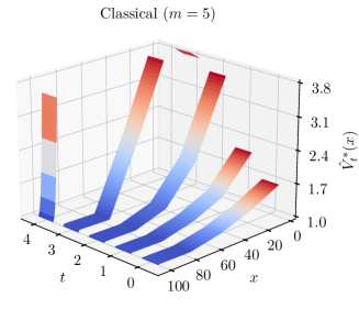
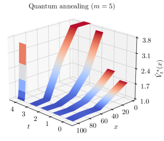
Figure 5: Approximated optimal value functions for each time step with the underlying approximation task of curve fitting for the fitted value iteration accomplished classically (left) and by virtue of quantum annealing.

In Tab. 3, we display our results for the optimal policies obtain by means of the different solution strategies. We find that the grid-based solution is indeed less optimal than the analytical one, which is caused, as explained earlier, by the discretization and forcing off-grid values onto on-grid ones. On the other hand, the solutions using a fitted value iteration are nearly identical with the analytical solution, which is the optimal one for $\alpha=1000$. Moreover, using a QUBO solved on a quantum annealer for the curve fitting in course of the value function approximation yields the same optimal policy than carrying out the fitting classically. Also, on the level of the individual optimal expansion coefficients $c_{j}^{\ast}$ at each nontrivial time step, shown in Tab. 4, we find that quantum annealing delivers, within limits, promising and practically useable results. The difference compared to the classically obtained coefficients is around/below ten percent. For the sake of a visual grasp, in the left (right) diagram of Fig. 5 we display the approximated optimal value function at each time step with the underlying curve fitting done classically (with quantum annealing).

$t=3$	$c_{0}^{\ast}$	$c_{1}^{\ast}$	$c_{2}^{\ast}$	$c_{3}^{\ast}$	$c_{4}^{\ast}$
Classical	$3.826$	$4.370$	$2.601$	$1.025$	$1.047$
Quantum	$3.936$	$3.969$	$2.781$	$0.969$	$1.125$
$\varepsilon_{\textup{rel}}$ [%]	$2.88$	$9.18$	$6.92$	$5.46$	$7.45$

$t=2$	$c_{0}^{\ast}$	$c_{1}^{\ast}$	$c_{2}^{\ast}$	$c_{3}^{\ast}$	$c_{4}^{\ast}$
Classical	$3.608$	$2.009$	$1.228$	$1.011$	$1.022$
Quantum	$3.875$	$1.969$	$1.156$	$1.031$	$1.031$
$\varepsilon_{\textup{rel}}$ [%]	$7.40$	$1.99$	$5.86$	$1.98$	$0.88$

$t=1$	$c_{0}^{\ast}$	$c_{1}^{\ast}$	$c_{2}^{\ast}$	$c_{3}^{\ast}$	$c_{4}^{\ast}$
Classical	$2.164$	$1.445$	$1.164$	$1.002$	$1.015$
Quantum	$2.000$	$1.344$	$1.156$	$1.031$	$0.938$
$\varepsilon_{\textup{rel}}$ [%]	$7.58$	$6.99$	$0.69$	$2.89$	$7.59$

$t=0$	$c_{0}^{\ast}$	$c_{1}^{\ast}$	$c_{2}^{\ast}$	$c_{3}^{\ast}$	$c_{4}^{\ast}$
Classical	$1.675$	$1.353$	$1.125$	$0.997$	$1.011$
Quantum	$1.563$	$1.344$	$1.156$	$1.063$	$0.969$
$\varepsilon_{\textup{rel}}$ [%]	$6.69$	$0.67$	$2.76$	$6.62$	$4.15$

Table 4: Expansion coefficients of the approximated optimal value function obtained classically and via quantum annealing.

V Summary and conclusions

Finding optimal speed profiles is an optimization problem that grows exponentially in time. Dynamic programming tames the combinatorial explosion of trajectories by solving the problem backward in time. The state-dependent optimal value function as a solution of the Bellman equation solves the problem linearly in the number of time steps but it requires a grid-based exploration of the entire state space. If the dimension of the latter is high, the well-known phenomena of “curse of dimensionality” poses a severe obstacle, particularly for large real-world use cases. An approximation of the optimal value function and thus its continuous representation mitigates the rounding error that occurs in the discrete grid-based setup.

Such approximations can often be reduced to curve fitting in one dimension. In this work, we formulated least-squares curve fitting, where we allowed for a rather general approximator in form of a finite linear combination of standardized (basis) functions, as a QUBO that is suited to be solved with quantum annealing. For simple functions/data points, we found that quantum annealing in its current state is in principle able to deliver comparable results to a classical computer. However, regardless of the choice of basis functions, curve fitting tasks that result in a QUBO size larger than about $60\times 60$ (i.e., with about 60 logical variables or more) cannot be solved accurate enough on a D-Wave annealer yet. The reason for that is the difficult low-energy landscape of the resulting Ising Hamiltonian.

In general, optimization problems formulated in terms of a QUBO can be modified by fine-tuning the penalty coefficients of the constraints in order to manipulate these landscapes in a proper way [54]. In our case, however, such an approach is not possible because the values of the QUBO matrix entries are solely fixed by the to-be-approximated data and the basis functions used for the approximator. Furthermore, the embedding of a floating point number on a quantum annealer might also contribute to an already complicated low-energy landscape.

Though quantum annealing devices promise a large number of qubits, attention should be paid to how many direct connections exist between the physical qubits. If one needs many interconnected variables, logical qubits must be created from several physical ones. We found that basis functions with support on the whole real line, e.g., all polynomials, result in a highly-connected QUBO matrix that is difficult to embed into the working graph of the annealer. However, we are confident that this issue will vanish eventually in the near future because of the advances in the ongoing development of quantum annealing hardware.

Nevertheless, the quantum annealing-oriented curve fitting principally works. Toward a real-word use case, it is for example possible to solve problems—albeit still in an exploratory fashion—within the topic of just-in-time navigation using that approach for approximating the value function in the Bellman equation of dynamic programming.

As a final remark, there are many other ways to approximate functions using a quantum computer. A promising approach is described in Ref. [55], which employs parameterized quantum circuits on a gate-based quantum computer using partial Fourier series. This seems to work with fewer qubits but the training process is significantly different. There are also ways to fit curves on a photonic quantum computer, see, e.g., Ref. [56]. There, the approximator is a variational quantum circuit built as an continuous-variable architecture that encodes quantum information in continuous degrees of freedom.