Causal Graph Discovery with Retrieval-Augmented Generation based Large Language Models

Abstract

Causal graph recovery is essential in the field of causal inference. Traditional methods are typically knowledge-based or statistical estimation-based, which are limited by data collection biases and individuals’ knowledge about factors affecting the relations between variables of interests. The advance of large language models (LLMs) provides opportunities to address these problems. We propose a novel method that utilizes the extensive knowledge contained within a large corpus of scientific literature to deduce causal relationships in general causal graph recovery tasks. This method leverages Retrieval Augmented-Generation (RAG) based LLMs to systematically analyze and extract pertinent information from a comprehensive collection of research papers. Our method first retrieves relevant text chunks from the aggregated literature. Then, the LLM is tasked with identifying and labelling potential associations between factors. Finally, we give a method to aggregate the associational relationships to build a causal graph. We demonstrate our method is able to construct high quality causal graphs on the well-known SACHS dataset solely from literature.

Causal Graph Discovery with Retrieval-Augmented Generation based Large Language Models

Yuzhe Zhang¹                        Yipeng Zhang^*$\dagger$1                        Yidong Gan^{$*$1,2 1}Data61, CSIRO ²University of Sydney ³University of New South Wales Sydney, Australia                        Lina Yao^$\dagger$1,3                        Chen Wang^$\dagger$1

1 Introduction

Estimating causal effect between variables from observational data is fundamental to problems in many domains including medical science Höfler (2005), social science Angrist et al. (1996), and economics Imbens and Rubin (2015); Yao et al. (2021). It enables reliable decision-making from complex data with entangled associations.

There are two main frameworks for causal inference: the potential outcome framework Rubin (1974) and the structural causal model (SCM) Pearl (1995). Directed Graphical Causal Models (DGCMs) Pearl (2000); Spirtes et al. (2001) is a powerful SCM method for representing and analyzing the causal relationships among factors. Causal graphs, which are integral to DGCMs, visually depict the hypothesized causal connections between nodes (factors) with directed edges.

Causal graph recovery Spirtes and Glymour (1991) usually seeks information from domain knowledge or data to uncover the structure of causal graphs. The task is often done through Causal Discovery (CD) Glymour et al. (2019) methods using a statistical estimation-based approach through observational data analysis when interventions or randomized experiments are not viable. Various algorithms along this line Spirtes et al. (2001); Chickering (2002); Shimizu et al. (2006); Sanchez-Romero et al. (2018) utilize statistical tests to assess associational relationships between factors as evidence to infer causal connections. Consequently, the reliability of these algorithms is affected by the quality of data, which can be compromised by issues such as measurement error Zhang et al. (2017) and selection bias Bareinboim et al. (2014). Furthermore, the unmeasured confounders and assumptions underlying the construction of causal models, such as the Gaussian data distributions, may not reflect the complexity of real-world scenarios. These shortcomings contribute to the susceptibility of CD methods to biases arising from both the data collection process and the model assumptions, underscoring the need for careful consideration and validation of the methods used in causal inference.

Recently, to mitigate the limitations of data quality in statistical estimation-based causal graph recovery tasks, Large Language Models (LLMs) Zhao et al. (2023) have been employed for causal graph recovery Zhou et al. (2023) in two main ways: directly outputting causal graphs or assisting in refining causal graphs generated by statistical or ML-based solutions. A straightforward method directly queries LLMs about every possible pair of factors Choi et al. (2022); Long et al. (2022); Kıcıman et al. (2023) to recover causal graphs. To solve the high complexity issue, Jiralerspong et al. (2024) proposed a breadth-first search approach to reduce the number of required queries. However, such methods require LLMs to have extensive background knowledge and robust causal reasoning skills, which are still being critically assessed Zečević et al. (2023). Alternatively, Vashishtha et al. (2023); Ban et al. (2023) employ LLMs to inject domain causal knowledge into statistical estimation-based methods, yet similar issues exist with these methods.

To address these challenges, we propose to recover causal connections by information extracted from a knowledge base containing related literature that contains valuable insight hidden in datasets about associational/causal relationships among variables. By leveraging LLMs to accomplish the information extraction from large document databases, we introduce the LLM Assisted Causal Recovery (LACR) method, which harnesses the collective insights from a large corpus of scientific literature. Instead of relying on LLMs’ causal reasoning capability, our approach leverages the Retrieval Augmented Generation (RAG) Lewis et al. (2020); Borgeaud et al. (2022) of LLMs to systematically analyze and extract relevant information from a comprehensive collection of research papers. Since the quality of the causal relationships existing in the literature varies, we utilize LLMs to extract associational relationships from related scientific literature, which are further used to induce causal relationships. Moreover, LACR is purely data-driven: we do not rely on task-specific knowledge for document retrieval or prompt design, and therefore, it can serve as a causal graph recovery tool for generic tasks.

LACR first retrieves relevant text chunks from the aggregated literature, and then, the LLM is tasked with identifying and reasoning the associational relationships between factors. Subsequently, we construct a causal graph where each node is a factor and each edge represents a causal connection between two factors. The causal connection is derived from associations identified by the LLM.

This methodology provides a more structured and less biased approach to inferring causal relationships, as it is grounded in a broader evidentiary base and subject to systematic validation. The robustness of our solution is further enhanced by the selection of a compatible knowledge base to the LLM that reduces the uncertainty of associational relation extraction from the LLM.

In summary, LACR shows a significant advancement in the causal graph recovery tasks, offering a method that is both grounded in scientific evidence and less susceptible to the biases that have historically challenged this area of research. We validate our method against the well-established SACHS dataset Sachs et al. (2005) and conduct a comparative analysis with existing statistical estimation-based CD algorithms, demonstrating its efficacy in general causal graph recovery tasks.

Our Contributions:

$\bullet$ We introduce a novel LLM-based causal graph recovery framework that leverages the extraction of associational relations from the scientific literature to reduce the bias inherent in traditional statistical estimation-based causal graph recovery methods.

$\bullet$ We give a generic LLM prompt structure to extract associational relations without relying on domain knowledge, instead, the domain knowledge is dynamically retrieved through RAG to form the context of LLM queries. We also apply self-consistency techniques when prompting the LLM to reduce the uncertainty in causal graph recovery.

$\bullet$ We conduct a comprehensive experimental evaluation of our framework using a real-world dataset under various parameter settings. Our approach outperforms baselines in terms of accuracy and reliability. Based on these experimental results, we offer insights and discuss potential strategies for further enhancing the efficacy of our solution.

2 Background

In this section, we introduce the preliminaries of the directed graphical causal models (DGCM) and causal graph recovery problems.

2.1 Directed Graphical Causal Models

A Directed Graphical Causal Model (DGCM) is a tuple $M=\langle G,P\rangle$. In the model, $G=\langle V,E\rangle$ is a Directed Acyclic Graph (DAG), also known as a causal graph, where the set of nodes $V=\{v_{1},\cdots,v_{n}\}$ represents random variables (with $|V|=n$), and $E\subseteq\{(v_{i},v_{j})\mid v_{i},v_{j}\in V\}$ is a set of directed edges that encode causal relationships. The joint probability distribution of all variables is denoted by $P$. Given a directed graph $G$, let $\ell=(v_{j_{1}},v_{j_{2}},\cdots,v_{j_{m}})$ denote a path, which is a sequence of distinct nodes, such that for each $i\in{1,2,\cdots,m-1}$, either $(v_{j_{i}},v_{j_{i+1}})\in E$ or $(v_{j_{i+1}},v_{j_{i}})\in E$. The subscript $i$ is the position of the node within $\ell$, and $m$ is the length of $\ell$.

A causal graph recovery task is to recover the directed graph $G$ given the set of variables $V$ with or without the joint probability distribution $P$. The feasibility of causal recovery tasks is usually subject to constraints and assumptions. As follows, we introduce the constraints and assumptions, based on which we design our method.

Constraints of causal graphs.

A causal graph subjects to a series of constraints. Especially, the directed edges specify the causal relationships between variables. Given $v_{i},v_{j}\in V$, if $(v_{i},v_{j})\in E$, $v_{i}$ is a direct cause of $v_{j}$. That is, fixing the other variables constant, varying the value of $v_{i}$ triggers a change of $v_{j}$’s value correspondingly, but not vice versa. This causal relationship thus entails the associational relationship between the variables, i.e., their marginal probability distributions $P(v_{i})$ and $P(v_{j})$ are correlated, which does not have the direction attribute. Notice that two variables can be associated even though they do not have direct causal relationship between each other. Typical examples are that the two variables have an indirect causal relationship through other variables, or they share the same parent node in $G$, which is usually called confounding in causal inference. See an example illustrating how we can induce associational relationships from a causal graph in Appendix A.1.

The structure of a causal graph should imply a conditional associational relationship between variables by a graphical constraint called d-separation Pearl (2000).

Definition 2.1 (d-separation)

A set of variables $S\subset V$ blocks a path $\ell$ if (i) $\ell$ contains at least one arrow-emitting variable belonging to $S$, or (ii) $\ell$ contains at least one collision variable ($v_{i}$ is a collision variable if $(v_{j_{i-1}},v_{j_{i}}),(v_{j_{i+1}},v_{j_{i}})\in E$, where $v_{j_{i-1}},v_{j_{i}}$, and $v_{j_{i+1}}$ are three adjacent nodes on $\ell$) that does not belong to $S$ and has no descendant belonging to $S$. If $S$ blocks all paths from variable $v_{i}$ to variable $v_{j}$, $S$ is said to d-separate $v_{i}$ and $v_{j}$. Then, $v_{i}$ and $v_{j}$ are independent conditioned on $S$.

Assumptions of causal graphs

The Markov property of the causal graph interprets that d-separation in causal graphs indicates conditional independence between variables. This is a necessary assumption based on which the DGCM works.

Assumption 2.2 (Causal Markov Assumption)

In each DGCM, each variable is independent of its non-descendants conditioned on its parents in the causal graph.

Practically, the joint probability distribution may contain additional independent information that is not induced by the d-separation constraints. Due to the sake of DGCM’s validation, we assume that there is no such additional independency information, formalized as the following assumption.

Assumption 2.3 (Causal Faithfulness Assumption)

In each DGCM, there is no additional conditional independence other than those entailed by the d-separation.

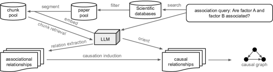
Figure 1: The work flow of LACR.

3 Methodology

Based on the above definitions of causal graphs, we are ready to introduce our solution. Traditional data-driven methodologies for causal graph recovery typically hinge on statistical estimation-based approaches. Based on Assumption 2.2 and Assumption 2.3, for each variable pair, such approaches rely on data to search variable sets that can d-separate (Definition 2.1) the pair, or in other words, whether the association between the pair can be blocked by other variables, to recover causal connections. However, they face challenges due to strict assumptions, data demands, and biases from confounding and measurement errors (See Appendix A.2 for a biased causal estimation example). These issues can compromise the accuracy of inferred causal relationships. To address these challenges, in this section, we propose the LLM Assisted Causal Discovery (LACR) method, leveraging a vast array of research literature to overcome the limitations of individual studies. The work flow of LACR is shown in Figure 1. LACR integrates diverse evidence and methodologies to verify the blockability of the association between each pair of variables, to form a more reliable causal graph.

In the following, we first introduce how to extract associational relationships from the literature and then verify the blockability of the extracted associational relationships to induce causal relationships.

3.1 Extract Association

With the above target to extract the association between each variable pair indicated in documents and verify its blockability, we instruct LLM to verify not only whether each pair of variables are associated, but also the association type that has different blokability. By the intuition of d-separation, we divide the association between two variables $v_{i}$ and $v_{j}$ into the following three types:

1. Independent: The absence of reported associations in the literature, or evidence of non-existence of association implies independence between the two variables.

2. Indirect Associated: A reported association which is triggered or linked by other variables in the literature implies indirect association between the two variables.

3. Direct Associated: A reported association that always exist even though we control any other variables constant in the literature implies direct association between the two variables.

We then design an association context (see the original prompt in Appendix A.6) as part of the query prompt for the LLM to understand the intuition of each of the above association types, as well as their common representation in the literature. Thereafter, for each pair of variables $v_{i}$ and $v_{j}$, we let LLM to read each retrieved document $c$ (see Section 3.3.1 for details of document retrieval), and verify the association between $v_{i}$ and $v_{j}$ (denoted by $R_{ij}$) (see Section 3.3.2 for details of querying LLM) as one of the following options and give additional information when applicable:

1. Independent: Chunk $c$ suggests that $v_{i}$ and $v_{j}$ are independent. We denote this association type as $R_{c}=\perp$).

2. Indirectly Associated: Chunk $c$ suggests that $v_{i}$ and $v_{j}$ are indirectly associated through one or more intermediary variables. When LLM selects this option, it is also instructed to give a list of the intermediary variables $INT$. This association type is denoted as $R_{c}=\mathsf{IA}(INT)$.

3. Directly Associated: Chunk $c$ suggests that $v_{i}$ and $v_{j}$ are directly associated, denoted as $R_{c}=\mathsf{A}$.

4. Unknown: Chunk $c$ does not provide clear information about the relationship, denoted as $R_{c}=\mathsf{U}$.

3.2 From Association To Causation: Causation Verification

Now, we are ready to recover the edges of the causal graph. Based on Assumption 2.2 and Assumption 2.3, we can induce that there is a causal link between a pair of variables if not all association between the pair can be blocked by other variables (Definition 2.1). Apparently, each association type that we defined in Section 3.1 has a deterministic blokability. Independence indicates that no association exists, or equivalently in terms of blokability, it indicates any association between the pair can be blocked. Direct association indicates that the extracted association cannot be blocked. However, from indirect association, we cannot deterministically infer whether the association between the pair of variables can be blocked or not. This is because an extracted indirect association cannot indicate the non-existence of direct association, even though an indirect association can be blocked.

1:  $G\leftarrow(V,E)$ where $E=\emptyset$

2:  for $(v_{i},v_{j})\in V\times V$ where $i\neq j$ do

3:     $chunks\leftarrow ChunkRetrieval((v_{i},v_{j}))$

4:     $d_{ij}\leftarrow 0$; $count_{ij}\leftarrow 0$

5:     for all $c\in chunks$ do

6:        if $R_{c}=\perp$ then

7:           $d_{ij}=d_{ij}-1$; $count_{ij}=count_{ij}+1$

8:        if $R_{c}=\mathsf{A}$ then

9:           $d_{ij}=d_{ij}+1$; $count_{ij}=count_{ij}+1$

10:        if $R_{c}=\mathsf{IA}(INT)$ and $|INT|==1$ then

11:           $v_{n}\leftarrow INT$

12:           $d_{i}=d_{in}+1$; $count_{in}=count_{in}+1$

13:           $d_{nj}=d_{nj}+1$; $count_{nj}=count_{nj}+1$

14:  for $(v_{i},v_{j})\in V\times V$ where $i\neq j$ do

15:     if $d_{ij}>0$ and $count_{ij}>=3$ then

16:        $E\leftarrow E\cup\{(v_{i},v_{j})\}$

17:  return $G$

Algorithm 1 Causation Existence Verification

Notice that direct association and independence are two conflicting association types in terms of blockability, but indirect association is not. Therefore, we use a voting process (Algorithm 1) to aggregate all chunks’ opinions for each variable pair and decide the existence of a causal link.

As we do not consider the causal direction in Algorithm 1, each pair of variables are symmetric, i.e., for $v_{i},v_{j}$, $d_{ij}=d_{ji}$ and $count_{ij}=count_{ji}$. For each variable pair, we first retrieve a limited number of the most relevant chunks by function $ChunkRetrieval$ (Line 3, see function details in Section 3.3.1). Then, if the chunk’s opinion is independent, it casts ballot $-1$, i.e., the association is blockable, in terms of the existence of a causal link between the pair (Lines 6-7); and if direct association, it casts $+1$, i.e., the association is non-blockable, (Lines 8-9). If the chunk indicates indirect association and there is only one intermediary variable $v_{n}$, it indicates that each of the pair of variables has a direct association with the intermediary , and thus, it casts $+1$ for both pairs $(v_{i},v_{n})$ and $(v_{n},v_{j})$ (Lines 10-13). We show more details of querying LLM association types in Section 3.3.2. Finally, we build an edge for each pair if the majority of chunks are supporting the non-blockable association and there are more than $3$ chunks providing evidence (Lines 14-16). Notice that the final decision is slightly biased towards $-1$, since the condition that direct association holds is strict.

3.3 Method Details

3.3.1 $ChunkRetrival$ in Algorithm 1

Document Pool Construction.

The Chunk Retrieval comprises two main steps: 1) an extensive scientific paper search to create a comprehensive literature pool; and 2) the chunk pool construction by chunking papers and filtering relevant chunks for efficient retrieval. Details are as follows:

1. We conduct a thorough search for each pair of variables $v_{i},v_{j}\in V$ in public databases using the query "[the name of $v_{i}$] and [the name of $v_{j}$]" to compile a literature pool that encompasses a broad spectrum of research findings, aiming to reduce data bias.

2. Papers are divided into chunks, which are then filtered to retain only those containing at least two variables’ names, ensuring relevance to our queries. These chunks are stored in a vector database to facilitate efficient retrieval for large variable sets. This ready-to-use vector store can enhance the efficiency of the following pairwise queries, especially when $|V|$ is large.

Chunk Selection.

For each variable pair $v_{i}$ and $v_{j}$, we query the LLM with "Are [the name of $v_{i}$] and [the name of $v_{j}$] associated?" using a subset of documents from our chunk pool. We employ an ensemble retriever that combines keyword-based and semantic-based methods to identify the most relevant chunks for each query. Chunks are ranked using the weighted reciprocal rank fusion algorithm, and we select a predetermined number of top chunks for further analysis. To ensure relevance, we discard any chunks that do not contain both variables in the query. This retrieval process is crucial for identifying chunks that provide evidence for the associational relationships between variable pairs

3.3.2 Query LLM

After retrieving the most relevant chunks from the chunk pool, we are ready to query LLM the associational relationship between the variable pair based on each retrieved document. As mentioned in Section 3.1, LLM needs to infer the relationship from one of four options. Specifically, LLM is tasked to recongnize the association type of pairs based on either LLM’s background knowledge (background-based), or the retrieved documents (document-based) by the following steps: Step 1. For each query based on either information resource, we ask LLM to first read the [association context] with a general [example] (see prompt and example details in Appendix A.6) to make LLM understand the intuition and typical representation of each association type defined in Section 3.1.
Step 2. For document-based queries, we ask LLM to read one of the [retrieved documents], but for background-based queries, we ask LLM to refer to its training data.
Step 3. Based on the above context, we ask LLM a question: “Are $v_{i}$ and $v_{j}$ associated? If yes, are they directly associated or indirectly associated?”, explain the reason, and specify the evidence shown in the document for document-based queries.
Step 4. We ask LLM to read its answer, explanation, and evidence, to ensure that its answer aligns with the [association context].
Step 5. We ask LLM to choose the final answer from “direct association”, “indirect association”, and “independent”. If the answer is “indirect association”, we ask LLM to list all intermediary variables that give rise to the association.

3.4 Causation Orientation

Now, we have linked each pair of variables that has a causal relationship, and hereby, we will decide the direction of each recovered causal link. For each variable pair $v_{i}$ and $v_{j}$, we use a similar strategy for the orienting process in the following steps:
Step 1. We ask LLM to read the [causal direction context] (see details in Appendix A.6) to make LLM understand the intuition of causal direction.
Step 2. For document-based queries, we ask LLM to read one of the [retrieved documents], but for background-based queries, we ask LLM to refer to its training data.
Step 3. Based on the above context, we let LLM answer the question: “Is $v_{i}$ a cause of $v_{j}$, or $v_{j}$ a cause of $v_{i}$?", explain the reason, and specify the evidence shown in the document for document-based queries.
Step 4. We ask LLM to read its answer, explanation, and evidence, to ensure that its answer aligns with the [causal direction context].
Step 5. Ask LLM to choose the final answer from “$v_{i}$ is a cause of $v_{j}$” and “$v_{j}$ is a cause of $v_{i}$”.
For each edge, we aggregate each chunk’s opinion ($v_{i}\rightarrow v_{j}$ or $v_{i}\leftarrow v_{j}$) by a similar strategy in Algorithm 1, and decide the direction of each edge.

4 Experiments

In this section, we first introduce the ground truth datasets and how we collect three research literature pools. Then we introduce the settings of our solution and baselines. Finally, we evaluate the pruning and orienting results, respectively.

4.1 Experiment Data

4.1.1 Ground Truth Datasets

In our study, we conducted experiments utilizing two ground truth causal graphs, SACHS and BIOLOGIST, representing causal protein-signaling networks derived from Sachs et al. (2005). SACHS was constructed by incorporating biological domain knowledge to revise the causal graph output by the application of Bayesian network analysis to multivariate flow cytometry data. BIOLOGIST corresponds to a consensus causal graph, which is widely accepted by the biological research community as a current representation of protein-signaling interactions. Both of them contain the same 11 variables (proteins).

4.1.2 Research Literature Pools

In our experiment, we prepare three literature pools, namely the PubMed, the Sachs, and the Full, for our solution LACR.

1. PubMed (P): We collected 340 abstracts and 177 full papers from official APIs of the medical science research database PubMed PubMed and PubMed Central Central .
2. Sachs (S): The papers in this pool are manually downloaded. A part of the papers are the reference papers of Sachs et al. (2005). However, the reference papers cannot cover all variables in $V$, and hence, we manually search and download additional papers to cover all variables in $V$. In total, this pool contains 38 papers, and half of them are the reference papers of Sachs et al. (2005).
3. Full (F): To construct this literature pool, for each pair of variables $v_{i},v_{j}\in V$, we search “$v_{i}$ and $v_{j}$” on PubMed, and manually download the top 5 English papers. Note that there might be overlapped papers in the search results of different variable pairs, and thus the total number of papers is fewer than 275.

Notice that Sachs may present selection bias in the paper retrieving process. However, this does not necessarily do harm to our result, since this kind of literature pool can be seen as a systematic literature review, which represents the state of the art of the task. We may reduce the noise of the input for LACR by using such literature pools.

4.2 Our Solution

LLM and Embedding.

The LLM we use is Google’s Gemini Pro. The ensemble retriever is constructed based on two distinct text representation models with equal weighting: BGE Xiao et al. (2023) for the dense representation, and Okapi BM25 Robertson et al. (2009) for the sparse representation. The embedded chunks were stored and indexed in a Chroma vector store. We set the chunk sizes of 1000 tokens with overlapping sizes of 150 tokens.

Query strategies.

We use two strategies to query LLM the association types:
1. Single query (SQ): For each chunk, we only query LLM once, with setting the temperature to $0$.
2. Multiple queries (MQ): We set LLM’s temperature to $0.2$ to allow a mild level of randomness. Then, for each chunk, we first query LLM three times, and select the association type with the most support. If there is a tie, we conduct one more query until the tie is broken. If the final decision is an indirect association, we only list the intermediary variables that are at least extracted twice. This technique enables self-consistency check Wang et al. (2022) for uncertain reduction.

Compared Methods.

We compare LACR with two statistic-based CD methods, Sachs and FASK.

LACR has adjustable implementation by the combination of three distinct literature pools (P, S, and F), and two query strategies (MQ and SQ). We denote a specific implementation as "Pools(Aggregation)." For example, P(SQ) employs literature pool P with the single query aggregation method, whereas F+P+S(MQ) represents a comprehensive LACR configuration that integrates all three literature pools and utilizes the multiple queries aggregation method.

Sachs (Sachs et al. (2005)) employs a Bayesian optimization to process 5400 data records for the 11 variables in $V$, by iterating the optimization for 500 DAGs. They include edges that appear in at least 85% DAGs.

The FASK method, detailed in Ramsey and Andrews (2018), implements the Fast Adjacency Skewness (FASK) algorithm Sanchez-Romero et al. (2018) to process a larger dataset containing 7,466 records, which includes nine additional variables, referred to as interventional variables). Due to the inability to replicate the exact results from from Ramsey and Andrews (2018), we illustrate the result of our implementation as "FASK", and the original result reported from Ramsey and Andrews (2018) as "FASK(report)."

Evaluation Metrics

We separately measure the performances of the pruning and the orienting, by using the same metrics in Ramsey and Andrews (2018). In the pruning process, we count the true positive ($\mathsf{TP}$) as the number of edges that are in both the evaluated graph and the ground truth graph. Similarly, we assess false positives ($\mathsf{FP}$), and false negatives ($\mathsf{FN}$). Then, we calculate adjacency precision (AP) as $\frac{\mathsf{TP}}{\mathsf{TP}+\mathsf{FP}}$ and adjacency recall (AR) as $\frac{\mathsf{TP}}{\mathsf{TP}+\mathsf{FN}}$, reflecting the accuracy and completeness of edge recovery, respectively. Based on the AP and AR, we also compute the F1 score. Additionally, we measure the number of different edges (DE), given by $\mathsf{FP}+\mathsf{FN}$, to quantify the total error in edge identification.

For the orienting process, we compute the metrics slightly differently. For each edge in the output causal graph, we consider it a true positive ($\mathsf{TP}$) edge if it is in the ground truth causal graph and has the same direction, otherwise, it is a false positive ($\mathsf{FP}$) edge. Then, we compute the AP, AR and the F1 score for each output causal graph based on this revised counting method.

4.3 Evaluation

Model	SACHS			BIOLOGIST
	AP(%)	AR(%)	F1(%)	AP(%)	AR(%)	F1(%)
Sachs	88.24	83.33	85.71	76.47	81.25	78.79
FASK	64.71	61.11	62.86	58.82	62.50	60.61
FASK (report)	73.68	77.78	75.68	63.16	75.00	68.57
P(SQ)	37.84	77.78	50.91	35.14	81.25	49.06
P(MQ)	81.25	72.22	76.47	75.00	75.00	75.00
P+S(SQ)	52.00	72.22	60.47	48.00	75.00	58.54
P+S(MQ)	83.33	55.56	66.67	75.00	56.25	64.29
P+S+F(SQ)	52.63	55.56	54.05	47.37	56.25	51.43
P+S+F(MQ)	43.75	77.78	56.00	40.62	81.25	54.17

Table 1: Comparative analysis of causal graph recovery. Overall highest performances and LACR’s highest performances are emphasized in bold.

Model	SACHS	BIOLOGIST
Sachs	5	7
FASK	13	13
FASK(report)	9	11
P(SQ)	27	27
P(MQ)	8	8
P+S(SQ)	17	17
P+S(MQ)	10	10
F(SQ)	19	17
F(MQ)	17	15
F+P+S(SQ)	17	17
F+P+S(MQ)	22	22

Table 2: Comparison of the total number of different edges in causal graph recovery. Two overall lowest DE are emphasized in bold.

4.3.1 Causation Existence Verification

In this section, we compare the experimental results of various CD methods against two types of ground truth datasets and illustrate the result in Table 1.

To Sachs’ truth (SACHS).

From the experimental results with SACHS ground truth, we illustrate four observations. First, Sachs’s method achieves the highest performance in AP, AR and F1, with values of 88.24%, 83.33% and 85.71%, respectively. This may be attributed to the method’s optimization process being tailored to the characteristics of the dataset it was originally designed to analyze.

Second, our solutions utilizing MQ consistently outperform SQ counterparts in F1. This suggests that aggregating information from multiple queries can lead to more robust decision making, as it allows for the integration of diverse perspectives and reduces the likelihood of relying on potentially anomalous results from a single query.

Third, a large literature pool does not necessarily provide a better performance. In fact, the opposite is often true. A possible reason is that the PubMed pool is classical and was used in the training of LLMs, which provides LLMs with a better understanding. Consequently, the model may be better equipped to extract relevant information and make accurate predictions when drawing from this familiar dataset.

Last, among all LACR models, P(MQ) stands out with the best performance, surpassing all the other baselines except for the Sachs model. This superior performance can potentially be attributed to the aforementioned familiarity of the language model with the PubMed pool, and MQ further enhances this success by increasing the chances of generating correct answers.

To biological truth (BIOLOGIST).

In this part, we evaluate the experimental results using the BIOLOGIST causal graph as the ground truth. We have the following observations.

First, in terms of the F1 score, Sachs’ method still outputs the best result, with AP 76.47%, AR 81.25%, and F1 score 78.79%. LACR’s P(MQ) model follows, reaching the values of AP, AR, and F1 scores of 75%, 75%, and 75%, respectively. All metrics of LACR’s P(MQ) result consistently surpass FASK, except an equal AR to the reported FASK. This suggests that the combination of a well-curated literature pool and the multiple queries strategy is highly effective in accurately capturing causal connections as validated by both computational and biological expertise.

Second, the multiple queries (MQ) strategy outperforms their single query (SQ) counterparts by an average of 11.48%. It implies that extracting information from various sources produces a more accurate and reliable causal model.

Third, comparing the evaluations to SACHS and to BIOLOGIST, LACR exhibits stability. Two reported baseline methods’ results experience a decline on all metrics, however, in contrast, LACR’s P(MQ) model shows slight improvement on AR and consistent DE. This shows that, by leveraging the aggregated knowledge, our solutions have the potential to be better positioned to align with the domain expert understanding of causal relationships, leading to a stable performance compared to baselines that may not utilize such a knowledge-driven framework.

4.3.2 Orienting Evaluation (BIOLOGIST)

With each of the above generated undirected graphs (the pool and query strategy used to generate each undirected graph is specified in column “Model” in Table 3 and Table 4), we ask LLM to orient each edge based on retrieved chunks from different pool combinations with the (MQ) strategy. We present the experimental results against the SACHS (Table 3) and the BIOLOGIST (Table 4) causal graphs.

To SACHS

First, as for F1 score, the best models are Sachs (first, F1 score 82.35%), reported FASK (second, F1 score 71.79%), and LACR’s P(MQ) using P+S and P+S+F (third, F1 score 68.75%). Notice that after orientation, the reported FASK exceeds LACR’s P(MQ) because of its accurate causal direction determination.

Second, observe that all models’ performance weakens, however, especially, LACR’s average performance mostly reduces, with a high variance. This indicates that LACR’s extracted causal information’s quality considerably varies.

To BIOLOGIST

First, the Sachs model still stands out with the highest F1 score of 75%, followed by P(MQ) using P+S and P+S+F as the orientation literature pools (F1 score 70.97%).

Second, consistent with the trend observed in the causation existence verification results, model P(MQ)’s performance metrics (using P+S and P+S+F) based on the BIOLOGIST ground truth are stable, with a slight improvement on the F1 scores, compared to the results against the SACHS ground truth (Table 3). This improvement suggests that our methods are more closely aligned with the expert knowledge and consensus represented in the BIOLOGIST dataset, which may contribute to enhanced performance.

Overall, when comparing the performance across the three literature pools in both Tables 3 and 4, we find that all three exhibit similar effectiveness in guiding the LLMs to predict edge orientations. However, the pool combining P+S shows a slight edge, outperforming the other two pools. It might be due to the complementary strengths of the combined literature sources. Together they provide a more holistic view of the domain knowledge required for causal inference.

Model	Pool	Precision(%)	Recall(%)	F1(%)
Sachs	-	82.35	82.35	82.35
FASK		52.94	56.25	54.55
FASK (report)		66.67	77.78	71.79
P(SQ)	P	10.81	50.00	17.78
P(MQ)		50.00	61.54	55.17
P+S(SQ)		24.00	54.55	33.33
P+S(MQ)		50.00	42.86	46.15
P+S+F(SQ)		10.53	20.00	13.79
P+S+F(MQ)		18.75	60.00	28.57
P(SQ)	P+S	10.81	50.00	17.78
P(MQ)		68.75	68.75	68.75
P+S(SQ)		44.00	68.75	53.66
P+S(MQ)		66.67	50.00	57.14
P+S+F(SQ)		36.84	46.67	41.18
P+S+F(MQ)		18.75	60.00	28.57
P(SQ)	P+S+F	13.51	55.56	21.74
P(MQ)		68.75	68.75	68.75
P+S(SQ)		24.00	54.55	33.33
P+S(MQ)		50.00	42.86	46.15
P+S+F(SQ)		26.32	38.46	31.25
P+S+F(MQ)		28.12	69.23	40.00

Table 3: Comparative analysis of the performance in orienting predictions by causal graph recovery methods: Sachs’s Model, FASK, and LACR, comparing to the SACHS causal graph.

Model	Pool	Precision(%)	Recall(%)	F1(%)
Sachs	-	70.59	80.00	75.00
FASK		47.06	57.14	51.61
FASK (report)		57.14	75.00	64.86
P(SQ)	P	8.11	50.00	13.95
P(MQ)		43.75	63.64	51.85
P+S(SQ)		24.00	60.00	34.29
P+S(MQ)		50.00	46.15	48.00
P+S+F(SQ)		10.53	22.22	14.29
P+S+F(MQ)		18.75	66.67	29.27
P(SQ)	P+S	10.81	57.14	18.18
P(MQ)		68.75	73.33	70.97
P+S(SQ)		44.00	73.33	55.00
P+S(MQ)		66.67	53.33	59.26
P+S+F(SQ)		31.58	46.15	37.50
P+S+F(MQ)		15.62	62.50	25.00
P(SQ)	P+S+F	10.81	57.14	18.18
P(MQ)		68.75	73.33	70.97
P+S(SQ)		20.00	55.56	29.41
P+S(MQ)		50.00	46.15	48.00
P+S+F(SQ)		21.05	36.36	26.67
P+S+F(MQ)		25.00	72.73	37.21

Table 4: Comparative analysis of the performance in orienting predictions by causal graph recovery methods: Sachs’s Model, FASK, and LACR, comparing to the BIOLOGIST causal graph.

4.4 Discussion

Declined performance from causation existence verification to causation orientation.

Though both tasks employ RAG to extract relationships from scientific literature, the causation existence verification (Section 4.3.1) extracts association relationships which has an overall higher accuracy and simplicity, comparing to the causal relationships that need complex inferences. Therefore, in the causation existence verification task, our method produces results close to statistical estimation-based CD methods, on average, and outperforms existing CD methods by taking proper inputs.

However, though our orientation method utilizes RAG to extract causal relationships from literature, it still relies on LLM’s causal reasoning capability, similar to existing LLM-based methods. This further indicates that LLM may not be well equipped with such reasoning capability.

Why does a larger literature pool negatively impact performance?

The negative impact of a larger literature pool on model performance is likely due to the following: Firstly, LLMs are often trained on well-known datasets such as PubMed, leading to better locating of information when paragraphs from these sources are used as the context. Other manually curated pools may contain papers not seen in model training, which results in higher uncertainty in relation extraction. Secondly, our approach incorporates the latest chemical and biological research, which might include findings not present in the SACHS and BIOLOGIST datasets, which are dated back to 2005.

5 Limitations

The first limitation is the dependency on the LLM, especially the relation extraction. While our results are promising, the performance of LACR could potentially be enhanced by further fine-tuning the LLMs with a comprehensive literature poolWadhwa et al. (2023). Another limitation is the method for orienting causal connections. In our current approach, we solely rely on the LLM for orientation. The reliability of this process could be improved by integrating established CD algorithms, such as the PC algorithm Spirtes et al. (2001), to analyze the associational relations extracted by the LLM.

6 Conclusion

In this work, we introduced the LLM Assisted Causal Recovery (LACR) method for causal graph recovery. By integrating the LLM and scientific literature pools, LACR has shown a potential to overcome the limitations inherent in traditional statistical estimation-based methodologies. We conducted experiments using real-world data against two broad consensus causal graphs. LACR not only showed its superiority in both graphs but particularly outperformed all baseline statistical estimation-based methods in the consensus graphs validated by domain experts. This demonstrated that by enhancing LLMs with relevant literature, LACR can achieve the causal reasoning capability comparable to that of experts in this field.

Appendix A Appendix

A.1 An Example of Inducing Association From A Causal Graph

Based on Assumption 2.2 and Assumption 2.3, given a causal graph, for each pair of factors $v_{i},v_{j}\in V$, we can induce their associational relation (conditioned on other factors) as follows.

For factors $v_{i}$ and $v_{j}$:
1. if there is no undirected path between them, then, they are statistically independent;
2. if there is only an undirected path between them and there is at least one collider on the path, then, the two factors are statistically independent;
3. if there is at least one undirected path between them, and no node on the path is a collider, then, the two factors are statistically associated;
4. there is an edge between them if and only if they are statistically associated conditioned on any factor set $S\subseteq V\setminus\{v_{i},v_{j}\}$.

We illustrate the above associational relation in Example A.1.

Figure 2: The causal graph of $A$, $B$, $C$, $D$ and $E$ in Example A.1.

Example A.1

Consider $5$ variables of which the causal graph is given in Figure 2.

There are two undirected paths between $A$ and $B$, i.e., $(A,D,B)$ and $(A,C,B)$, and we will discuss two cases where the direct path $(A,B)$ exists or not. First observe that there is no path between $E$ and any other variables, and therefore, we have that $E$ is independent from any other variables. If paths $(A,B)$ and $(A,D,B)$ do not exist, we have that variables $A$ and $B$ are independent from each other because the change of either variable will not cause any corresponding change of the other variable as $C$ is a collider.

Since there is no collider on path $(A,D,B)$, variables $A$ and $B$ are statistically associated. However, if conditioned on $D$, $A$ and $B$ are independent, we can conclude that there is no direct path (or edge) between $A$ and $B$. In this case, $\{D\}$ d-separates $A$ and $B$ (Definition 2.1). On the other hand, if $A$ and $B$ are still associated conditioned on $D$, there is a direct path between $A$ and $B$.

A.2 A Motivation for LACR: Selection Bias in CD Methods

Average treatment effect

Average treatment effect (ATE) is a frequently used measure of causation between two variables, the treatment $T\in V$ and the outcome $Y\in V$. Hereby, we consider binary treatment and outcome, i.e., $T\in\{0,1\}$ and $Y=\{0,1\}$. Intuitively, $T=1$ or $0$ indicates whether treatment is administered or not, and similarly, $Y=1$ or $0$ indicates whether an effect is observed or not. Given a causal graph, to obtain an appropriate ATE, we need to balance the effect of covariates on both the treatment and the outcome. The following Back-door criterion Pearl (2000) can be used to select such a set of covariates.

Definition A.2 (Back-door path)

Given $G=\langle V,E\rangle$, a back-door path $\ell_{b}$ from $T\in V$ to $Y\in V$ is a path $\ell_{b}=(T,v_{i_{1}},\cdots,v_{i_{k}},Y)$ that satisfies $(v_{i_{1}},T)\in E$.

A set $S$ of variables is admissible to obtain an appropriate ATE if the following conditions hold: 1) No element of S is a descendant of the treatment; and 2) The elements of $S$ block all “back-door” paths from the treatment to the outcome, i.e., all paths that end with an arrow pointing to the treatment.

Definition A.3 (Back-door criterion)

Given $G=\langle V,E\rangle$, a set $S\subseteq V$ satisfies the back-door criterion relative to a pair of variables $(T,Y)\in V$ if: (1) $\forall v\in S,v\text{ is not a descendant of }T$; (2) $S$ blocks every back-door path $\ell_{b}$ from $T$ to $Y$.

Then, for a set of covariates $S=\{s_{1},\cdots,s_{k}\}$ that satisfies the back-door criterion, we have that the ATE is:

$$\begin{split}ATE=&\sum_{s_{1},\cdots,s_{k}}P(s_{1},\cdots,s_{k})\\ &\left(P(Y=1\mid s_{1},\cdots,s_{k},do(T=1))\right.\\ &\quad\left.-P(Y=1\mid s_{1},\cdots,s_{k},do(T=0))\right)\end{split}$$ (1)

where $do(T)$ is intervention operator, i.e., enforce $T$ to be a specific value.

As follows, we show an example of data-driven methods’ vulnerability to a type of data bias, the so-called selection bias Bareinboim et al. (2014).

Figure 3: Causal graphs in Example A.4: left-the truth causal graph; right-recovered causal graph by the biased data.

Example A.4

Consider that we would like to investigate whether human gender ($G\in\{0,1\}$) is a cause of positive detection of a disease ($D\in\{0,1\}$), where human age ($A\in\mathbb{Z}_{\geq 0}$) is a covariate. Let $p_{G}$, $p_{A}$, and $p_{D}$ be the probability distribution of $G$, $A$, and $D$, respectively, and assume that the true causal graph of $X$, $Y$, and $Z$ is depicted as the left figure in Figure 3.

Generally speaking, human age and gender are associated because female has a longer average lifespan. Assuming that this association is only significant for $A\geq 60$, i.e., for the younger population than 60 years old, we cannot observe significant difference between the population of male and female.

Now we need to estimate the ATE of $G$ on $D$ by a dataset $D$, where in each sample of $D$, the value of $A$ is fewer than $60$. Then, by statistical test, we have that $G$ and $A$ are statistically independent from each other. Therefore, the recovered causal graph is depicted as the right figure in Figure 3.

Then, by dataset $D$, we estimate the ATE of $G$ on $D$ based on the biased causal graph as

$$\begin{split}\hat{ATE}=&P(d=1\mid do(g=1))-\\ &P(d=1\mid do(g=0)).\end{split}$$ (2)

However, based on the true causal graph, we should estimate the ATE of $G$ on $D$ as

$$\begin{split}\hat{ATE}^{*}=\sum_{a}p(a)(P(d=1\mid a,do(g=1))\\ -P(d=1\mid a,do(g=0))).\end{split}$$ (3)

We usually yield different values by Equation 2 and Equation 3.

A.3 Additional Experiment Details

The biological classic signaling network (Figure 4), Sachs’ truth causal graph (Figure 5) in Sachs et al. (2005).

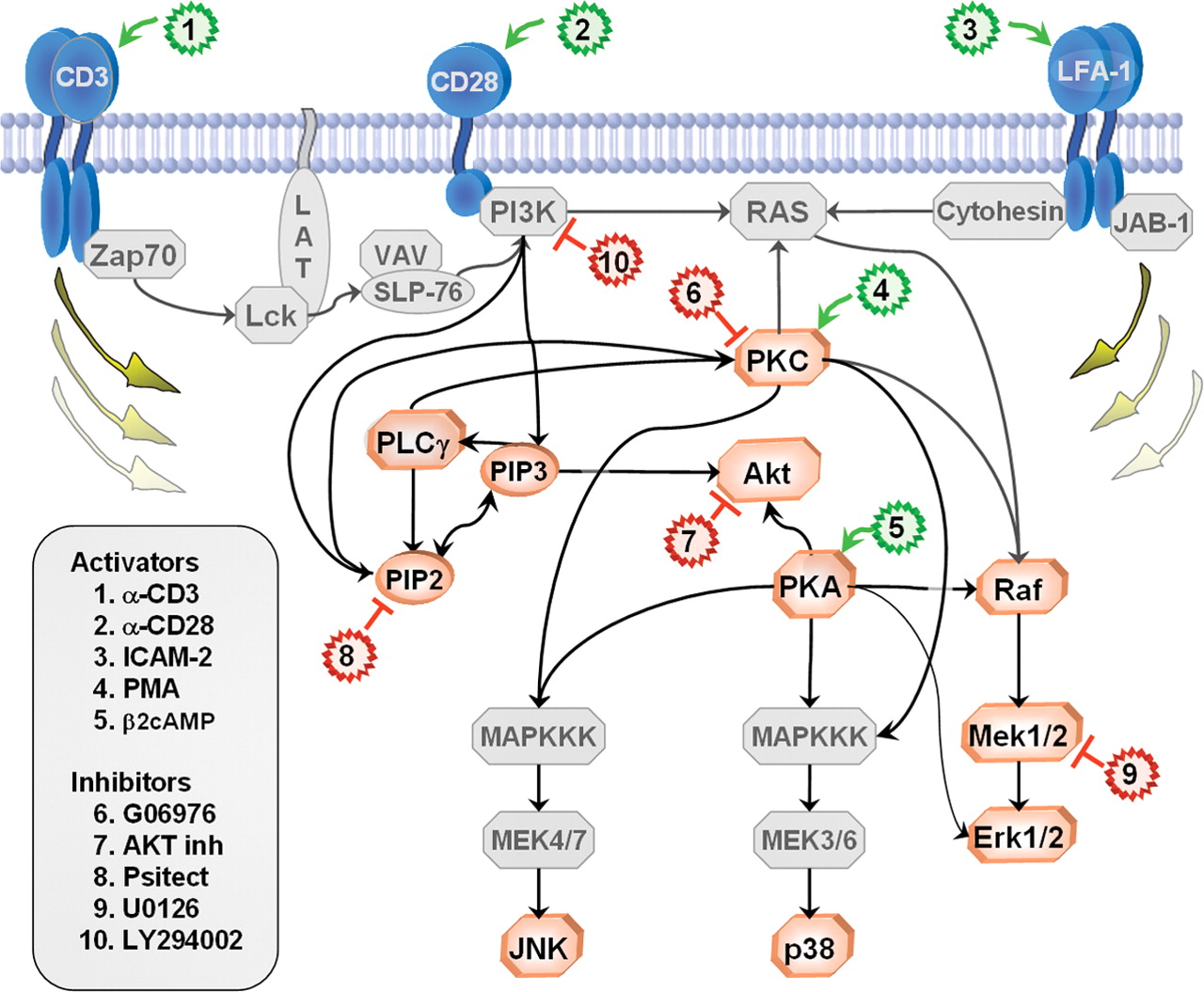
Figure 4: Biologists’ view of the causal protein-signaling graph.

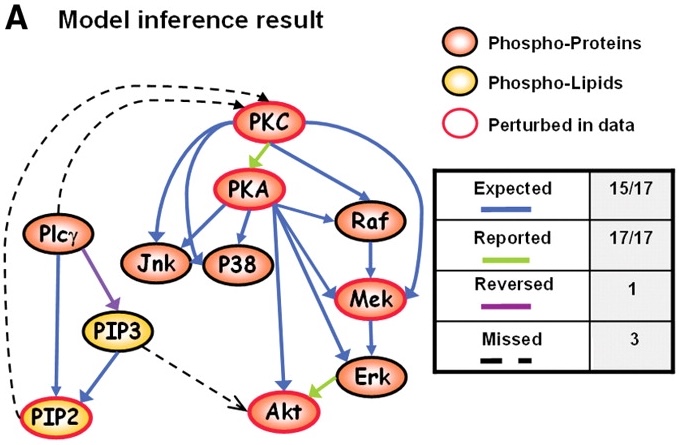
Figure 5: Sachs et al.’s view of the causal protein-signaling graph.

A.4 Additional Experimental Result

A.5 Causal Graphs

Causal graphs recovered by LACR with different combinations of input literature pools (PubMed, Sachs, and Full) and query strategies (SQ and MQ).

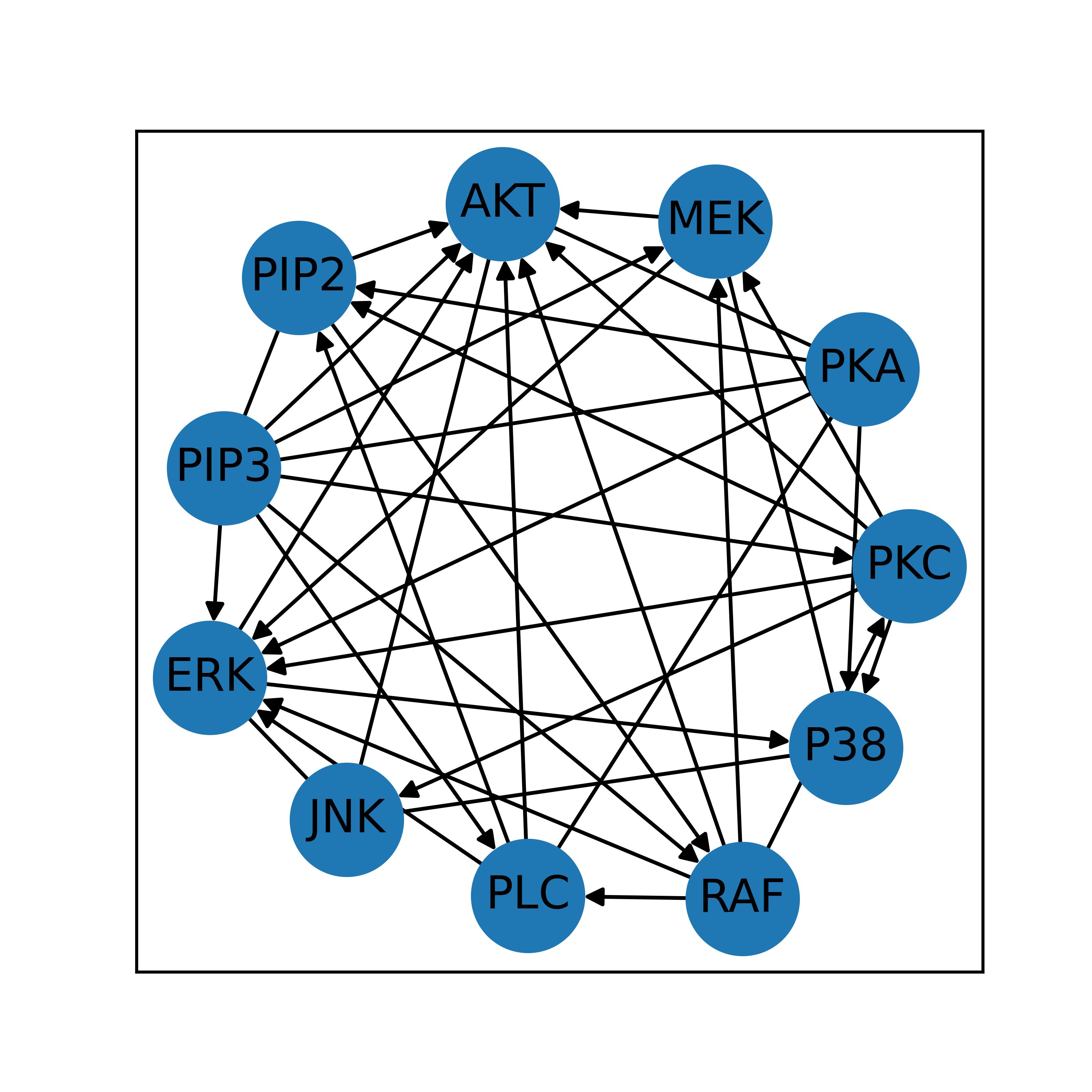
Figure 6: Causal graph recovered by LACR using PubMed(SQ) with PubMed(MQ) as the orienting query pool.

Figure 7: Causal graph recovered by LACR using PubMed(SQ) with PubMed+Sachs(MQ) as the orienting query pool.

Figure 8: Causal graph recovered by LACR using PubMed(SQ) with PubMed+Sachs+Full(MQ) as the orienting query pool.

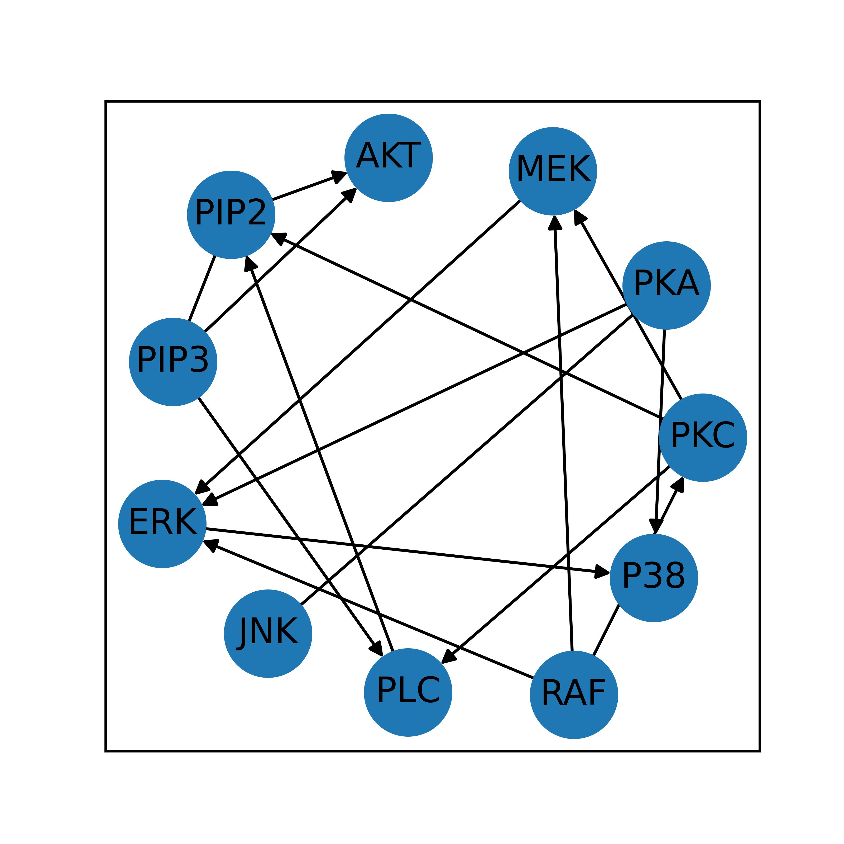
Figure 9: Causal graph recovered by LACR using PubMed(MQ) with PubMed(MQ) as the orienting query pool.

Figure 10: Causal graph recovered by LACR using PubMed(MQ) with PubMed+Sachs(MQ) as the orienting query pool.

Figure 11: Causal graph recovered by LACR using PubMed(MQ) with PubMed+Sachs+Full(MQ) as the orienting query pool.

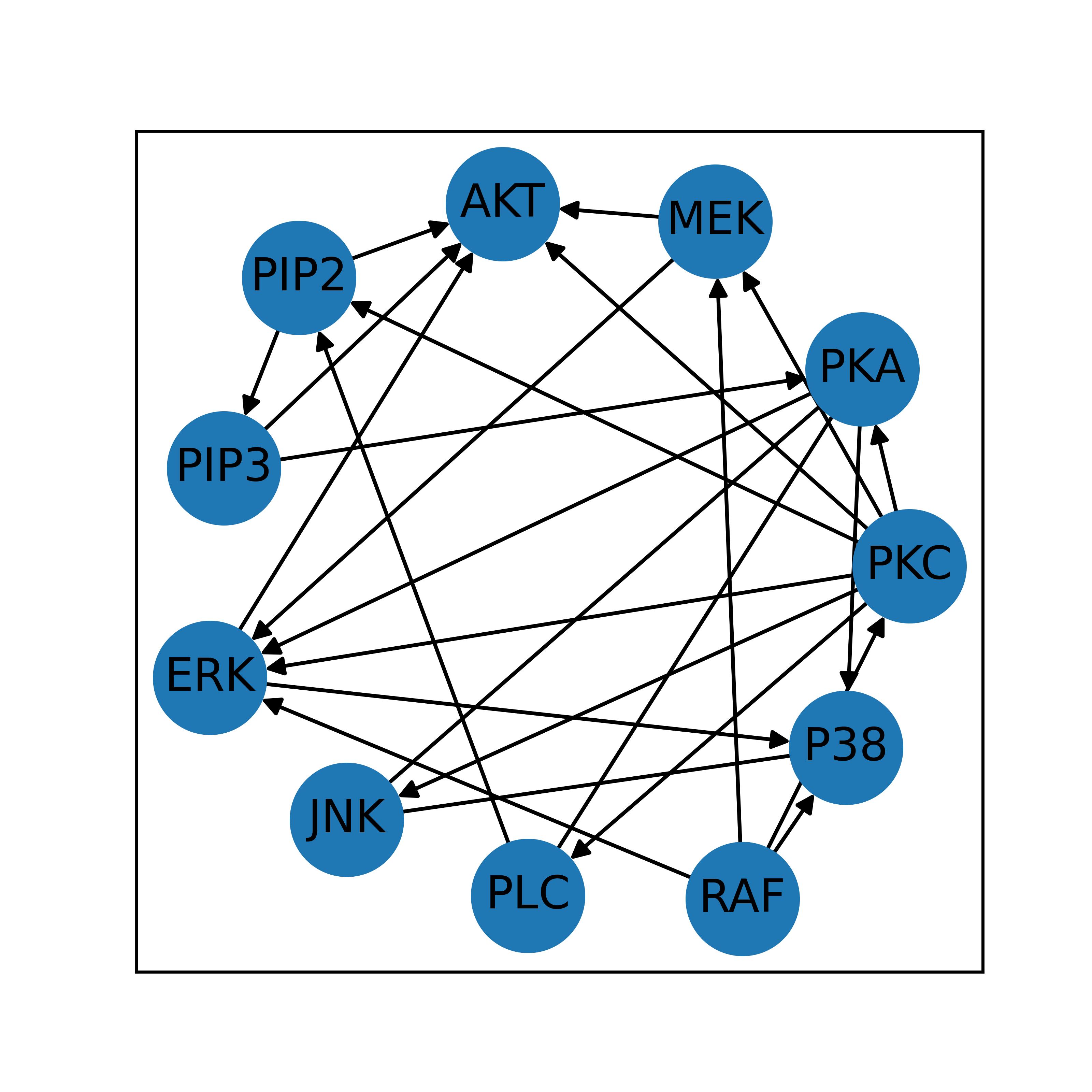
Figure 12: Causal graph recovered by LACR using PubMed+Sachs(SQ) with PubMed(MQ) as the orienting query pool.

Figure 13: Causal graph recovered by LACR using PubMed+Sachs(SQ) with PubMed+Sachs(MQ) as the orienting query pool.

Figure 14: Causal graph recovered by LACR using PubMed+Sachs(SQ) with PubMed+Sachs+Full(MQ) as the orienting query pool.

Figure 15: Causal graph recovered by LACR using PubMed+Sachs(MQ) with PubMed(MQ) as the orienting query pool.

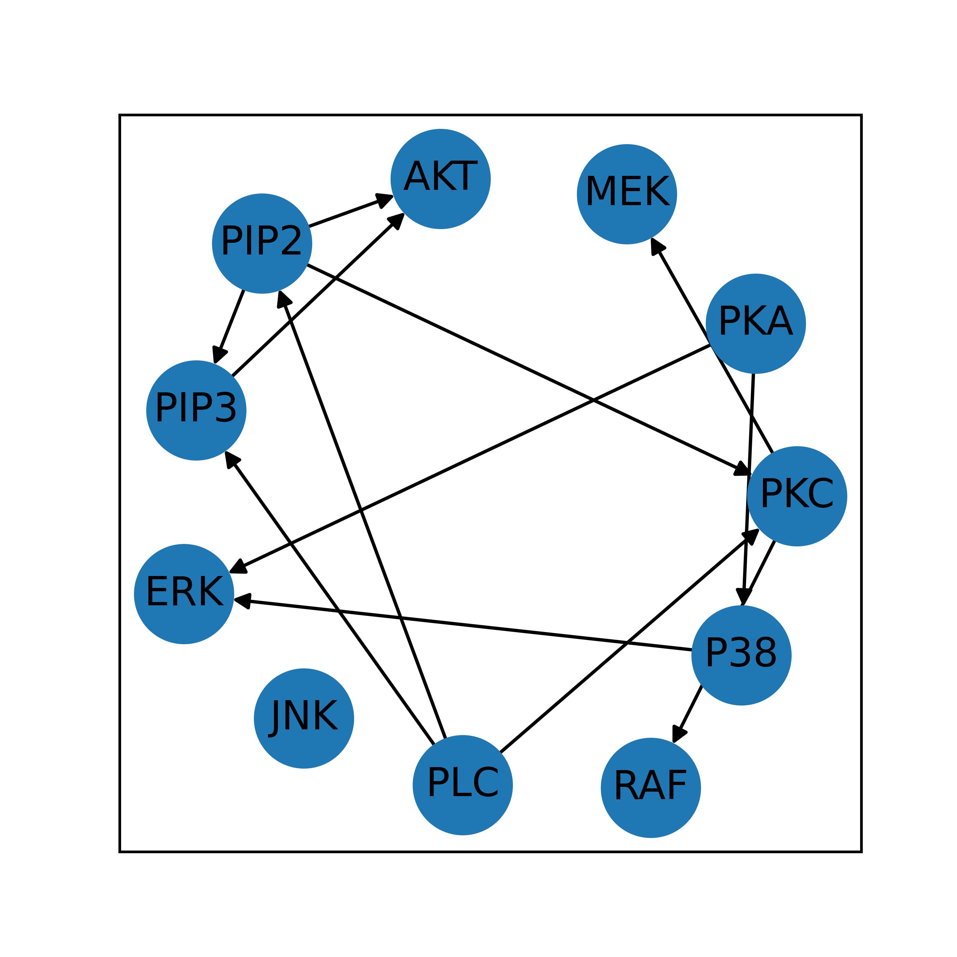
Figure 16: Causal graph recovered by LACR using PubMed+Sachs(MQ) with PubMed+Sachs(MQ) as the orienting query pool.

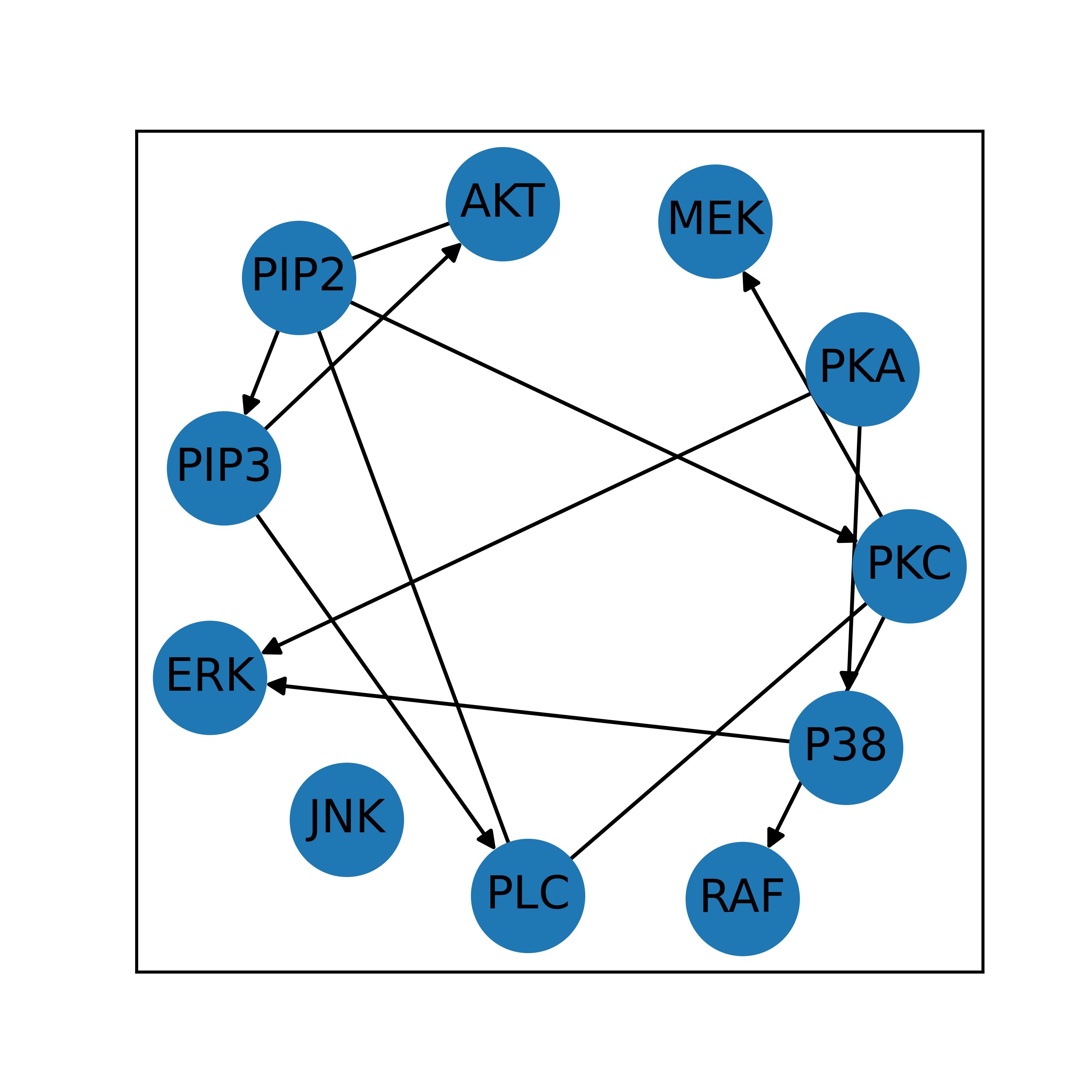
Figure 17: Causal graph recovered by LACR using PubMed+Sachs(MQ) with PubMed+Sachs+Full(MQ) as the orienting query pool.

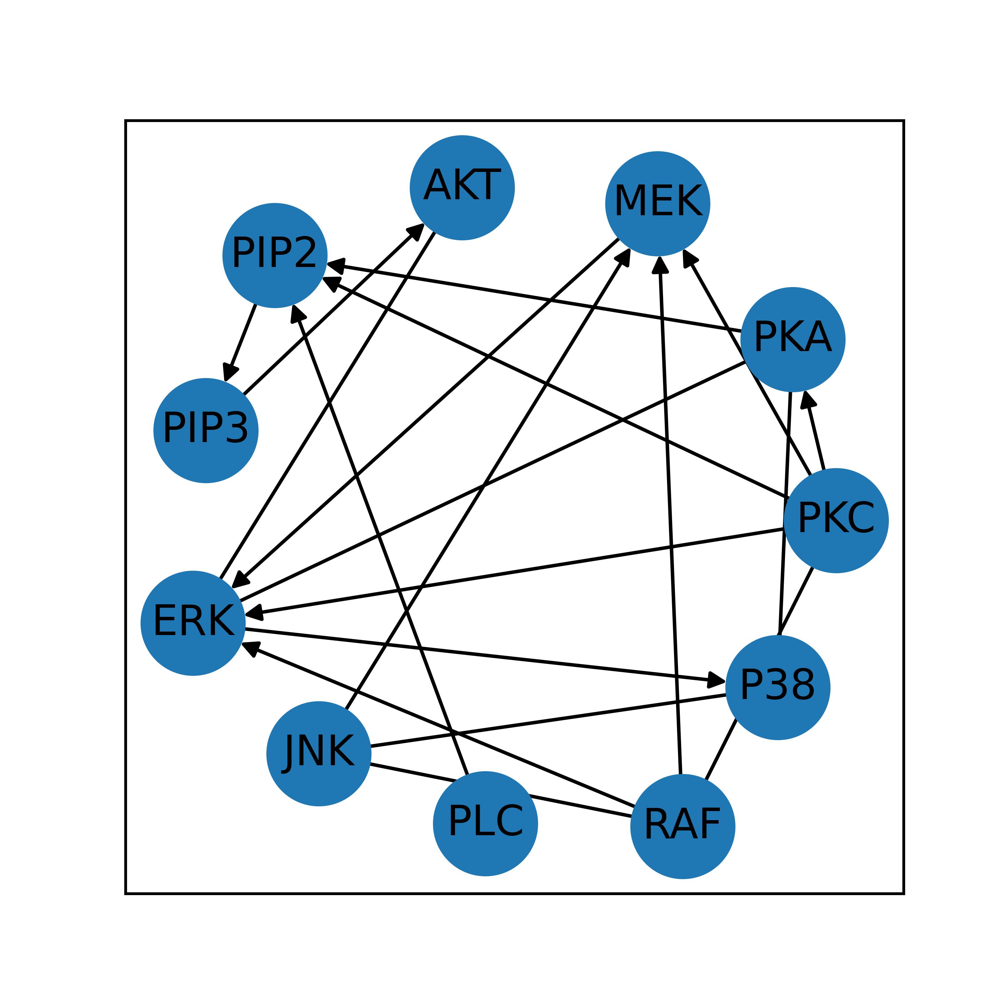
Figure 18: Causal graph recovered by LACR using PubMed+Sachs+Full(SQ) with PubMed(MQ) as the orienting query pool.

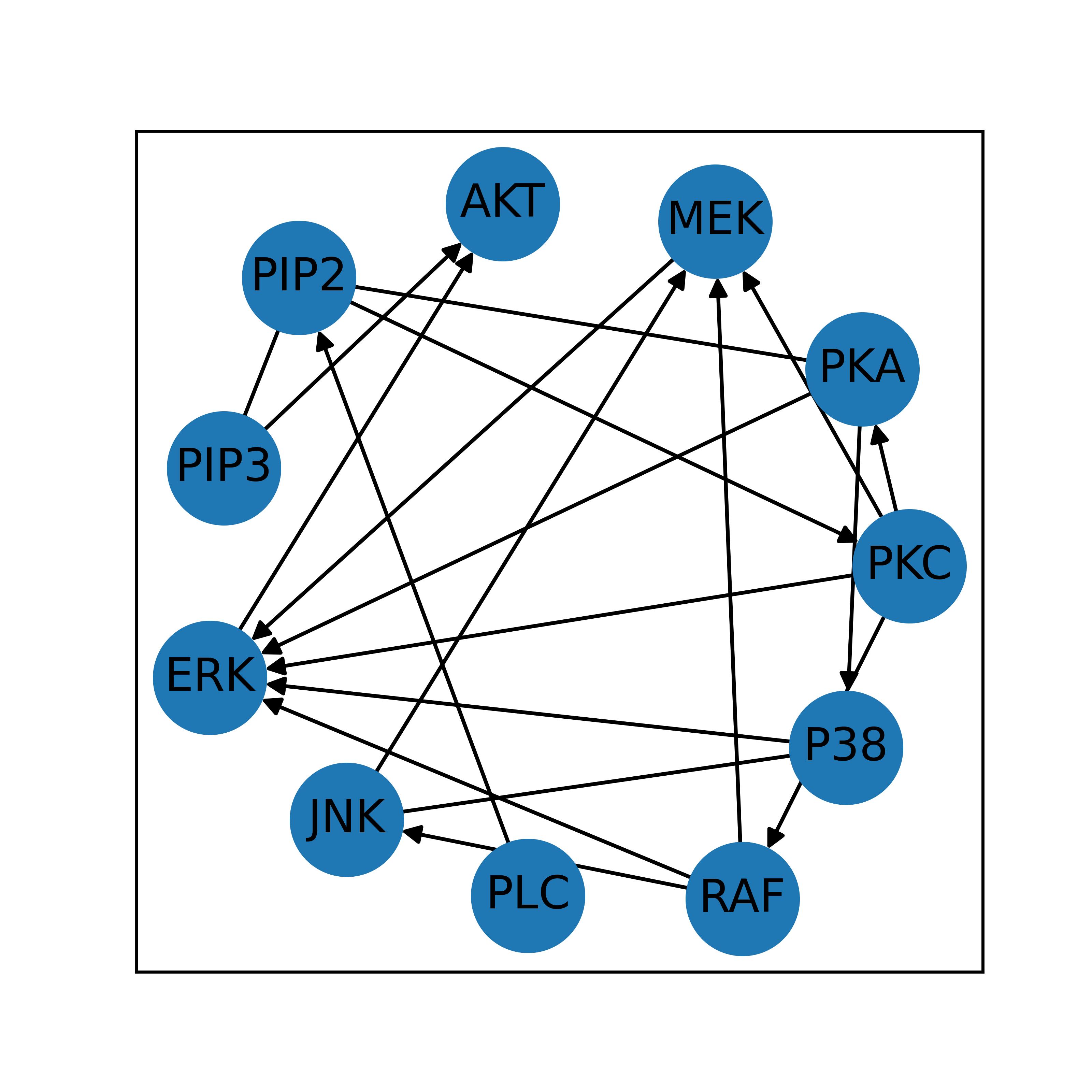
Figure 19: Causal graph recovered by LACR using PubMed+Sachs+Full(SQ) with PubMed+Sachs(MQ) as the orienting query pool.

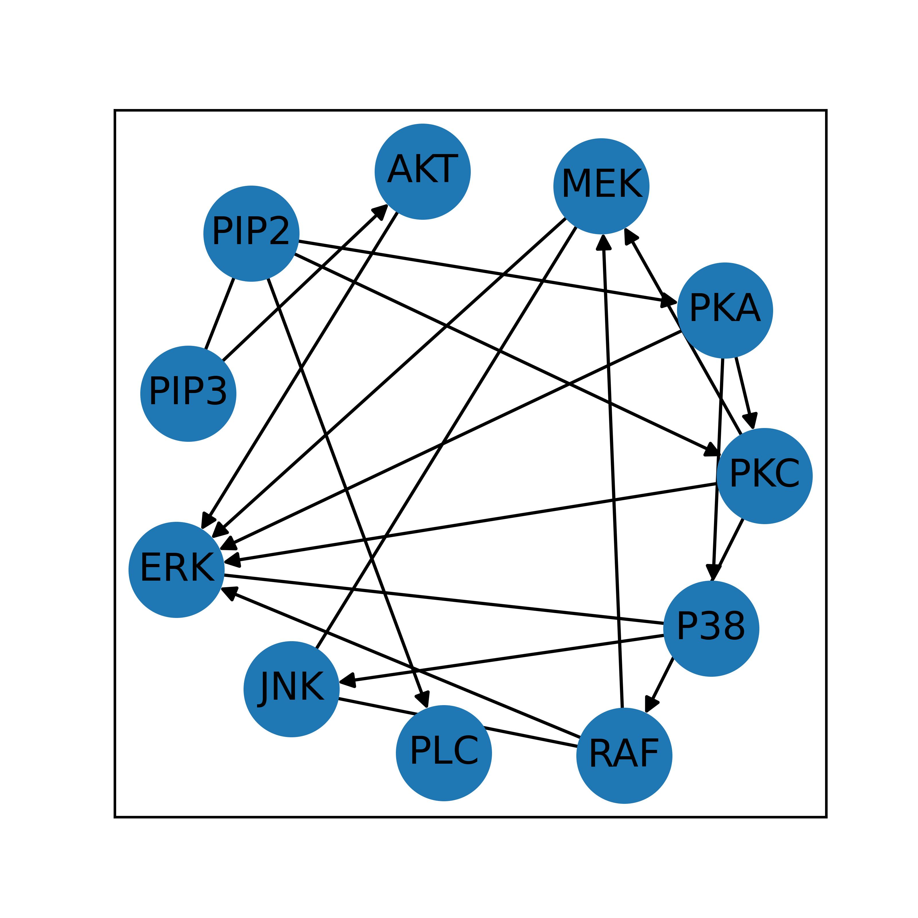
Figure 20: Causal graph recovered by LACR using PubMed+Sachs+Full(SQ) with PubMed+Sachs+Full(MQ) as the orienting query pool.

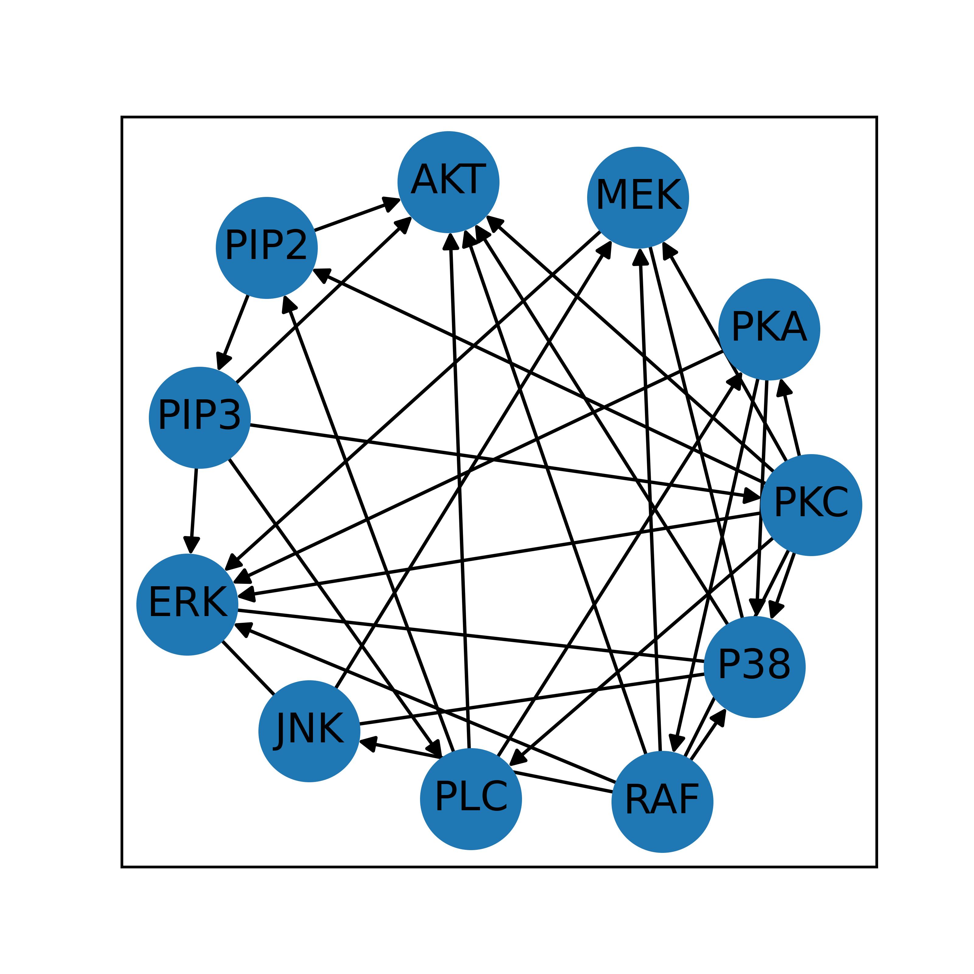
Figure 21: Causal graph recovered by LACR using PubMed+Sachs+Full(MQ) with PubMed(MQ) as the orienting query pool.

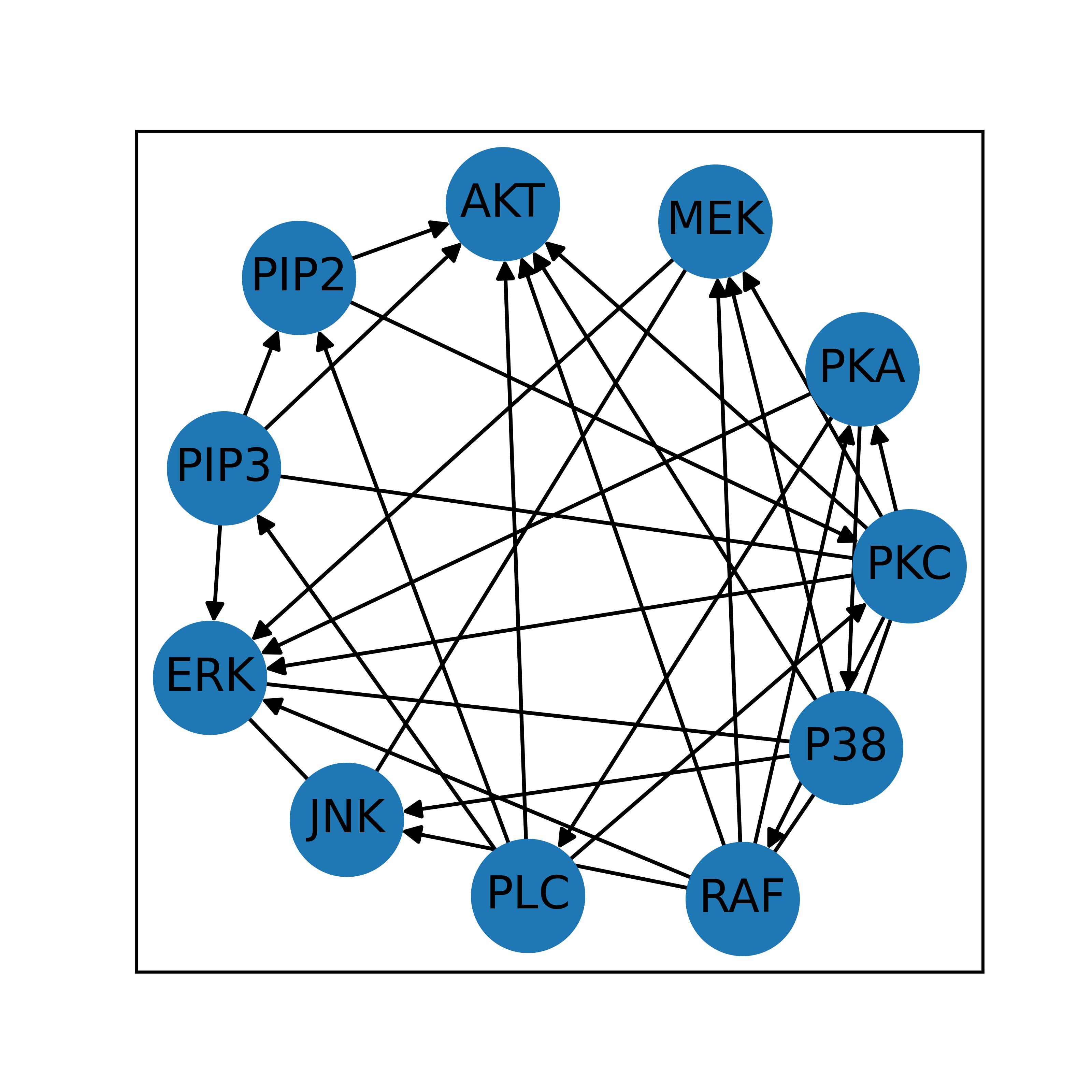
Figure 22: Causal graph recovered by LACR using PubMed+Sachs+Full(MQ) with PubMed+Sachs(MQ) as the orienting query pool.

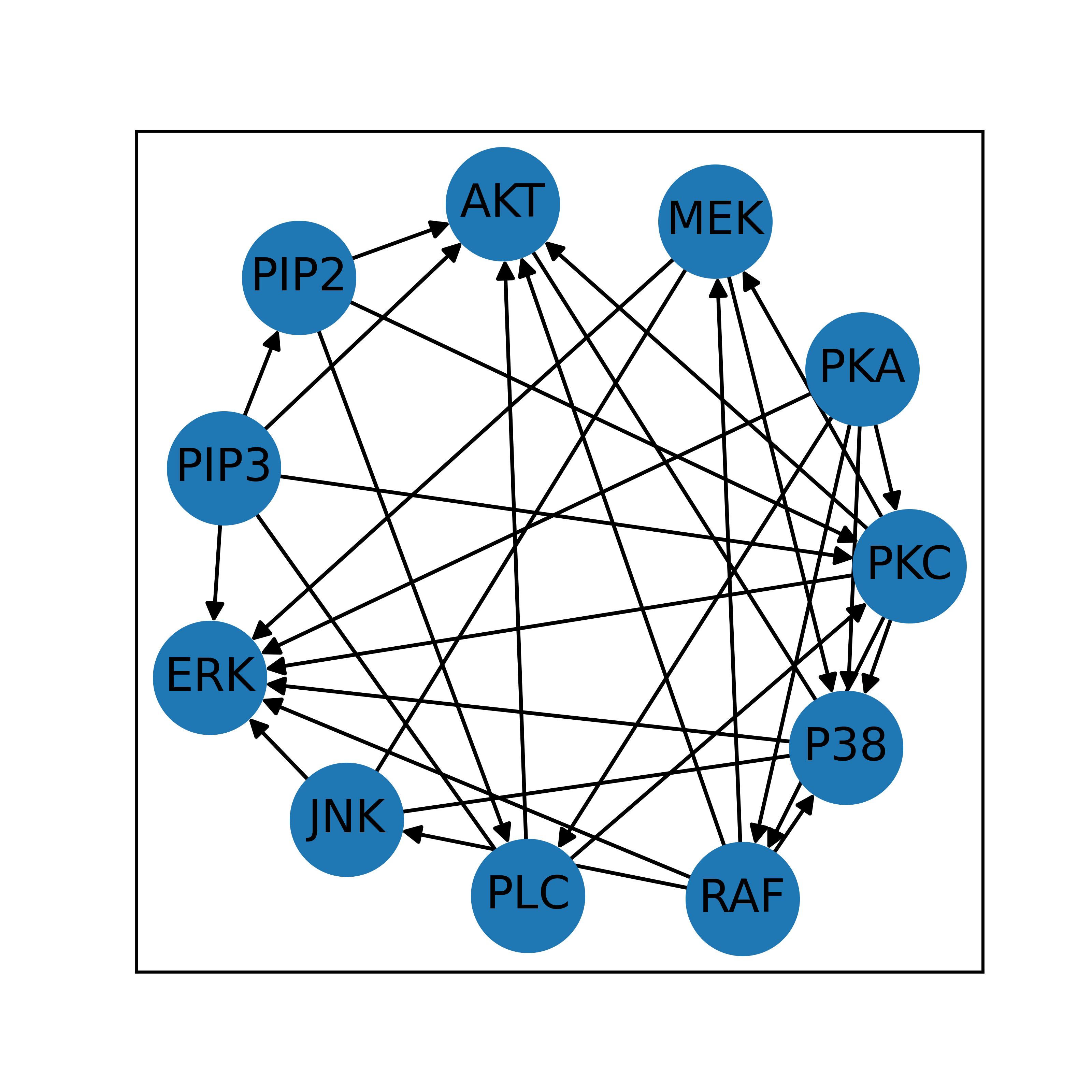
Figure 23: Causal graph recovered by LACR using PubMed+Sachs+Full(MQ) with PubMed+Sachs+Full(MQ) as the orienting query pool.

A.6 Prompts

Original prompts are described in Section 3.3.2. Section A.6.1 is the prompt to query LLM’s background knowledge. Section A.6.2 is the prompt to use LLM to extract associational relationships from retrieved chunks. Then, in Section A.6.3 and Section A.6.4, we give the prompts for the RAG-based orientation (Section 3.4) from LLM’s background knowledge and retrieved chunks.

A.6.1 Query LLM Associational Relationships (Background-Based Query)

⬇

As a scientific researcher, your task is to use your background knowledge to determine the association between two factors. Follow these steps:

1. Read the ’Context Information’ section (delimited by triple dollar signs) to understand the meaning of ’Association’.

2. Enhance your understanding by reading the ’Examples’ section.

3. Think step by step. With your background knowledge, write your thoughts regarding the given question, then select your answer from the multiple-choice options.

4. Before you respond, ensure your thoughts and answer align with all the information in the ’Context Information’ section.

5. Respond according to the expected format (delimited by triple backticks).

Context Information:

$$$

Consider two factors - A and B:

1. A and B are not associated if and only if A does not influence B and B does not influence A.

2. If either factor influences the other, then they are associated.

3. The fact that A does not influence B does not necessarily mean that B does not influence A.

4. You should never assume or infer that A and B are not associated unless this is explicitly stated in a document. It is possible that their relationship may sometimes be unknown.

5. Direct association refers to a scenario where one variable directly affects another without any intermediary variables.

6. Indirect association occurs when the effect of one variable on another is transmitted through one or more intermediary variables.

Consider there are factors other than A and B:

1. When a third factor, C, influences both A and B directly, then A and B are associated indirectly through C. If C only has an impact on one of the factors (A or B), then it is unknown if A or B are associated.

2. When both A and B influences C, it doesn’t mean that A and B are associated.

3. When A influences B, which in turn influences a third factor, C, then A and C are indirectly associated.

$$$

Examples:

Factor A: The quality of school facilities (e.g., libraries, sports fields)

Factor B: The effectiveness of the teaching methods

Factor C: Student academic performance

Factor D: If student likes to play game

Factor E: Student’s study time

In this example, the relationships are:

1. B directly affects C (Direct Association): The effectiveness of the teaching methods (Factor B) directly influences student academic performance (Factor C) without any other intemediatory factor.

2. D indirectly affects C via E (Indirect Association): When a student enjoys playing games (Factor D), it might reduce their available study time (Factor E), potentially impacting their academic performance (Factor C).

3. B does not affect A (Independent): The quality of school facilities (Factor A) is independent of the teaching methods (Factor B). The way teachers impart education doesn’t necessarily change or improve the physical resources like libraries or sports facilities.

4. Unknown if A affects C (Unknown): It’s uncertain whether the quality of school facilities (Factor A) has a direct impact on student academic performance (Factor C). While better facilities might provide a more conducive learning environment, their direct influence on academic performance isn’t clearly established in this scenario.

Question: What is relationship between {factorA} and {factorB}?

Expected Response Format:

“‘

Thoughts:

[Write your thoughts on the question]

Answer:

(A) Direct association

(B) Indirect association

(C) Independent

(D) Unknown

Intermediary Factors:

[Skip this if you did not choose B above. Otherwise list all factors involved in this indirect association relationship, each separated by a comma]

“‘

A.6.2 Query LLM Associational Relationships (Document-Based Query)

⬇

As a scientific researcher, your task is to analyse a document to determine the association between two factors. This is part of a controlled experiment; therefore, you should rely solely on the information provided in the document, not your background knowledge. Follow these steps:

1. Read the ’Context Information’ section (delimited by triple dollar signs) to understand the background of your task.

2. Enhance your understanding by reading the ’Examples’ section.

3. Read the given document thoroughly.

4. Think step by step. Write your thoughts regarding the given question, then select your answer from the multiple-choice options.

5. Before you respond, ensure your thoughts and answer align with all the information in the ’Context Information’ section.

6. Respond according to the expected format (delimited by triple backticks).

Context Information:

$$$

Consider two factors - A and B:

1. A and B are not associated if and only if A does not influence B and B does not influence A.

2. If either factor influences the other, then they are associated.

3. The fact that A does not influence B does not necessarily mean that B does not influence A.

4. You should never assume or infer that A and B are not associated unless this is explicitly stated in a document. It is possible that their relationship may sometimes be unknown.

5. Direct association refers to a scenario where one variable directly affects another without any intermediary variables.

6. Indirect association occurs when the effect of one variable on another is transmitted through one or more intermediary variables.

Consider there are factors other than A and B:

1. When a third factor, C, influences both A and B directly, then A and B are associated indirectly through C. If C only has an impact on one of the factors (A or B), then it is unknown if A or B are associated.

2. When both A and B influences C, it doesn’t mean that A and B are associated.

3. When A influences B, which in turn influences a third factor, C, then A and C are indirectly associated.

$$$

Examples:

Factor A: The quality of school facilities (e.g., libraries, sports fields)

Factor B: The effectiveness of the teaching methods

Factor C: Student academic performance

Factor D: If student likes to play game

Factor E: Student’s study time

In this example, the relationships are:

1. B directly affects C (Direct Association): The effectiveness of the teaching methods (Factor B) directly influences student academic performance (Factor C) without any other intermediary factor.

2. D indirectly affects C via E (Indirect Association): When a student enjoys playing games (Factor D), it might reduce their available study time (Factor E), potentially impacting their academic performance (Factor C).

3. B does not affect A (Independent): The quality of school facilities (Factor A) is independent of the teaching methods (Factor B). The way teachers impart education doesn’t necessarily change or improve the physical resources like libraries or sports facilities.

4. Unknown if A affects C (Unknown): It’s uncertain whether the quality of school facilities (Factor A) has a direct impact on student academic performance (Factor C). While better facilities might provide a more conducive learning environment, their direct influence on academic performance isn’t clearly established in this scenario.

Document:

{document}

Question: What is relationship between {factorA} and {factorB}?

Expected Response Format:

“‘

Document Identifier: XXX

Thoughts:

[Write your thoughts on the question after reading the document]

Answer:

(A) Direct association

(B) Indirect association

(C) Independent

(D) Unknown

Reference:

[Skip this if you chose option D above. Otherwise, provide a supporting sentence from the document for your choice]

Intermediary Factors:

[Skip this if you did not choose B above. Otherwise list all factors involved in this indirect association relationship, each separated by a comma]

“‘

A.6.3 Query LLM to orient causal relationships (Background-Based Query)

⬇

As a scientific researcher, your task is to use your background knowledge to determine the causal relationship between two factors. Follow these steps:

1. Read the ’Context Information’ section (delimited by triple dollar signs) to understand the meaning of ’Causality’.

2. Enhance your understanding by reading the ’Examples’ section.

3. Think step by step. With your background knowledge, write your thoughts regarding the given question, then select your answer from the multiple-choice options.

4. Before you respond, ensure your thoughts and answer align with all the information in the ’Context Information’ section.

5. Respond according to the expected format (delimited by triple backticks).

Context Information:

$$$

Consider two factors - A and B:

1. A is a direct cause of B if A directly influences B or A directly activates B.

2. If A is not a cause of B, it does not mean that B is not a cause of A.

3. If A only influences B through other intermediary factors, then A is not a cause of B.

$$$

Examples:

Factor A: The effectiveness of the teaching methods

Factor B: Student academic performance

In this example, the relationships are:

1. A affects B (Causality): The effectiveness of the teaching methods (Factor A) directly influences student academic performance (Factor B). For instance, innovative and engaging teaching methods can lead to better understanding and retention of information by students, thereby improving their academic performance.

2. B does not affect A (Non-Causality): Any changes in the student academic performance (Factor B) will not have an direct impact on the effectiveness of the teaching method (Factor A).

Question: What is causal relationship between {factorA} and {factorB}?

Expected Response Format:

“‘

Thoughts:

[Write your thoughts on the question]

Answer:

(A) {factorA} is a direct cause of {factorB}

(B) {factorB} is a direct cause of {factorA}

(C) Unknown

“‘

A.6.4 Query LLM to orient causal relationships (Document-Based Query)

⬇

As a scientific researcher, your task is to analyse a document to determine the causal relationship between two factors. This is part of a controlled experiment; therefore, you should rely solely on the information provided in the document, not your background knowledge. Follow these steps:

1. Read the ’Context Information’ section (delimited by triple dollar signs) to understand the background of your task.

2. Enhance your understanding by reading the ’Examples’ section.

3. Read the given document thoroughly.

4. Think step by step. Write your thoughts regarding the given question, then select your answer from the multiple-choice options.

5. Before you respond, ensure your thoughts and answer align with all the information in the ’Context Information’ section.

6. Respond according to the expected format (delimited by triple backticks).

Context Information:

$$$

Consider two factors - A and B:

1. A is a direct cause of B if A directly influences B or A directly activates B.

2. If A is not a cause of B, it does not mean that B is not a cause of A.

3. If A only influences B through other intermediary factors, then A is not a cause of B.

$$$

Examples:

Factor A: The effectiveness of the teaching methods

Factor B: Student academic performance

In this example, the relationships are:

1. A affects B (Causality): The effectiveness of the teaching methods (Factor A) directly influences student academic performance (Factor B). For instance, innovative and engaging teaching methods can lead to better understanding and retention of information by students, thereby improving their academic performance.

2. B does not affect A (Non-Causality): Any changes in the student academic performance (Factor B) will not have an direct impact on the effectiveness of the teaching method (Factor A).

Document:

{document}

Question: What is causal relationship between {factorA} and {factorB}?

Expected Response Format:

“‘

Thoughts:

[Write your thoughts on the question]

Answer:

(A) {factorA} is a direct cause of {factorB}

(B) {factorB} is a direct cause of {factorA}

(C) Unknown

Reference:

[Provide a supporting sentence from the document]

“‘

References

- Angrist et al. (1996) Joshua D Angrist, Guido W Imbens, and Donald B Rubin. 1996. Identification of causal effects using instrumental variables. Journal of the American statistical Association, 91(434):444–455.
- Ban et al. (2023) Taiyu Ban, Lyvzhou Chen, Xiangyu Wang, and Huanhuan Chen. 2023. From query tools to causal architects: Harnessing large language models for advanced causal discovery from data.
- Bareinboim et al. (2014) Elias Bareinboim, Jin Tian, and Judea Pearl. 2014. Recovering from selection bias in causal and statistical inference. Proceedings of the AAAI Conference on Artificial Intelligence, 28(1).
- Borgeaud et al. (2022) Sebastian Borgeaud, Arthur Mensch, Jordan Hoffmann, Trevor Cai, Eliza Rutherford, Katie Millican, George Bm Van Den Driessche, Jean-Baptiste Lespiau, Bogdan Damoc, Aidan Clark, et al. 2022. Improving language models by retrieving from trillions of tokens. In International conference on machine learning, pages 2206–2240. PMLR.
- (5) PubMed Central. https://www.ncbi.nlm.nih.gov/pmc/.
- Chickering (2002) David Maxwell Chickering. 2002. Optimal structure identification with greedy search. Journal of machine learning research, 3(Nov):507–554.
- Choi et al. (2022) Kristy Choi, Chris Cundy, Sanjari Srivastava, and Stefano Ermon. 2022. Lmpriors: Pre-trained language models as task-specific priors. arXiv preprint arXiv:2210.12530.
- Glymour et al. (2019) Clark Glymour, Kun Zhang, and Peter Spirtes. 2019. Review of causal discovery methods based on graphical models. Frontiers in genetics, 10:524.
- Grofman et al. (1983) Bernard N. Grofman, Guillermo Owen, and Scott L. Feld. 1983. Thirteen theorems in search of the truth. Theory and Decision, 15:261–278.
- Höfler (2005) Marc Höfler. 2005. Causal inference based on counterfactuals. BMC medical research methodology, 5(1):1–12.
- Imbens and Rubin (2015) Guido W. Imbens and Donald B. Rubin. 2015. Causal Inference for Statistics, Social, and Biomedical Sciences: An Introduction. Cambridge University Press.
- Jiralerspong et al. (2024) Thomas Jiralerspong, Xiaoyin Chen, Yash More, Vedant Shah, and Yoshua Bengio. 2024. Efficient causal graph discovery using large language models.
- Kıcıman et al. (2023) Emre Kıcıman, Robert Ness, Amit Sharma, and Chenhao Tan. 2023. Causal reasoning and large language models: Opening a new frontier for causality. arXiv preprint arXiv:2305.00050.
- Lewis et al. (2020) Patrick Lewis, Ethan Perez, Aleksandra Piktus, Fabio Petroni, Vladimir Karpukhin, Naman Goyal, Heinrich Küttler, Mike Lewis, Wen-tau Yih, Tim Rocktäschel, et al. 2020. Retrieval-augmented generation for knowledge-intensive nlp tasks. Advances in Neural Information Processing Systems, 33:9459–9474.
- Long et al. (2022) Stephanie Long, Tibor Schuster, and Alexandre Piché. 2022. Can large language models build causal graphs? In NeurIPS 2022 Workshop on Causality for Real-world Impact.
- Pearl (1995) Judea Pearl. 1995. Causal diagrams for empirical research. Biometrika, 82(4):669–688.
- Pearl (2000) Judea Pearl. 2000. Causality: Models, Reasoning and Inference. Cambridge University Press, New York.
- (18) PubMed. https://pubmed.ncbi.nlm.nih.gov/.
- Ramsey and Andrews (2018) Joseph Ramsey and Bryan Andrews. 2018. Fask with interventional knowledge recovers edges from the sachs model. arXiv preprint arXiv:1805.03108.
- Robertson et al. (2009) Stephen Robertson, Hugo Zaragoza, et al. 2009. The probabilistic relevance framework: Bm25 and beyond. Foundations and Trends® in Information Retrieval, 3(4):333–389.
- Rubin (1974) Donald B Rubin. 1974. Estimating causal effects of treatments in randomized and nonrandomized studies. Journal of educational Psychology, 66(5):688.
- Sachs et al. (2005) Karen Sachs, Omar Perez, Dana Pe’er, Douglas A Lauffenburger, and Garry P Nolan. 2005. Causal protein-signaling networks derived from multiparameter single-cell data. Science, 308(5721):523–529.
- Sanchez-Romero et al. (2018) Ruben Sanchez-Romero, Joseph D Ramsey, Kun Zhang, MR K Glymour, Biwei Huang, and Clark Glymour. 2018. Causal discovery of feedback networks with functional magnetic resonance imaging. bioRxiv, page 245936.
- Shimizu et al. (2006) Shohei Shimizu, Patrik O Hoyer, Aapo Hyvärinen, Antti Kerminen, and Michael Jordan. 2006. A linear non-gaussian acyclic model for causal discovery. Journal of Machine Learning Research, 7(10).
- Spirtes and Glymour (1991) Peter Spirtes and Clark Glymour. 1991. An algorithm for fast recovery of sparse causal graphs. Social Science Computer Review, 9(1):62–72.
- Spirtes et al. (2001) Peter Spirtes, Clark Glymour, and Richard Scheines. 2001. Causation, Prediction, and Search. The MIT Press.
- Vashishtha et al. (2023) Aniket Vashishtha, Abbavaram Gowtham Reddy, Abhinav Kumar, Saketh Bachu, Vineeth N Balasubramanian, and Amit Sharma. 2023. Causal inference using llm-guided discovery.
- Wadhwa et al. (2023) Somin Wadhwa, Silvio Amir, and Byron Wallace. 2023. Revisiting relation extraction in the era of large language models. In Proceedings of the 61st Annual Meeting of the Association for Computational Linguistics (Volume 1: Long Papers), pages 15566–15589, Toronto, Canada. Association for Computational Linguistics.
- Wang et al. (2022) Xuezhi Wang, Jason Wei, Dale Schuurmans, Quoc Le, Ed Chi, Sharan Narang, Aakanksha Chowdhery, and Denny Zhou. 2022. Self-consistency improves chain of thought reasoning in language models. arXiv preprint arXiv:2203.11171.
- Xiao et al. (2023) Shitao Xiao, Zheng Liu, Peitian Zhang, and Niklas Muennighof. 2023. C-pack: Packaged resources to advance general chinese embedding. arXiv preprint arXiv:2309.07597.
- Yao et al. (2021) Liuyi Yao, Zhixuan Chu, Sheng Li, Yaliang Li, Jing Gao, and Aidong Zhang. 2021. A survey on causal inference. ACM Transactions on Knowledge Discovery from Data (TKDD), 15(5):1–46.
- Zečević et al. (2023) Matej Zečević, Moritz Willig, Devendra Singh Dhami, and Kristian Kersting. 2023. Causal parrots: Large language models may talk causality but are not causal. Transactions on Machine Learning Research.
- Zhang et al. (2017) Kun Zhang, Mingming Gong, Joseph Ramsey, Kayhan Batmanghelich, Peter Spirtes, and Clark Glymour. 2017. Causal discovery in the presence of measurement error: Identifiability conditions. arXiv preprint arXiv:1706.03768.
- Zhao et al. (2023) Wayne Xin Zhao, Kun Zhou, Junyi Li, Tianyi Tang, Xiaolei Wang, Yupeng Hou, Yingqian Min, Beichen Zhang, Junjie Zhang, Zican Dong, et al. 2023. A survey of large language models. arXiv preprint arXiv:2303.18223.
- Zhou et al. (2023) Guanglin Zhou, Shaoan Xie, Guangyuan Hao, Shiming Chen, Biwei Huang, Xiwei Xu, Chen Wang, Liming Zhu, Lina Yao, and Kun Zhang. 2023. Emerging synergies in causality and deep generative models: A survey.