Linear Dynamics-embedded Neural Network for Long-Sequence Modeling

Abstract

The trade-off between performance and computational efficiency in long-sequence modeling becomes a bottleneck for existing models. Inspired by the continuous state space models (SSMs) with multi-input and multi-output in control theory, we propose a new neural network called Linear Dynamics-embedded Neural Network (LDNN). SSMs’ continuous, discrete, and convolutional properties enable LDNN to have few parameters, flexible inference, and efficient training in long-sequence tasks. Two efficient strategies, diagonalization and ${}^{\prime}\text{Disentanglement then Fast Fourier Transform (FFT)}^{\prime}$, are developed to reduce the time complexity of convolution from $O(LNH\max\{L,N\})$ to $O(LN\max\{H,\log L\})$. We further improve LDNN through bidirectional noncausal and multi-head settings to accommodate a broader range of applications. Extensive experiments on the Long Range Arena (LRA) demonstrate the effectiveness and state-of-the-art performance of LDNN.

I Introduction

Sequence modeling with long-range dependency is a crucial and challenging problem in many application fields of machine learning, e.g., natural language processing (NLP) [1], computer vision (CV) [2], and time series forecasting [3]. Extensive research has been conducted to mitigate this problem. Among various works, deep learning has shown its compelling ability in sequence modeling.

Recurrent Neural Networks (RNNs) employ a recursive architecture with a memory mechanism that compresses history information. Compared with standard feedforward neural networks, RNNs can make flexible inferences at any time length. The gradient vanishing and exploding problem make them challenging to train [4]. Subsequent works, like LSTM [5] and bidirectional RNN [6], have attempted to address these issues. However, the sequential nature of RNNs makes them unable to be trained efficiently in a parallel setting because of the backpropagation across the time chain.

Transformer with attention mechanism avoids the problems in RNNs and realizes parallel computing [7]. Thereafter, it achieves remarkable success in NLP, CV, and time series [8]. However, the quadratic complexity of length prevents the Transformer from exhibiting efficient performance in modeling long sequences. Many efficient variants have been introduced with reduced complexity to tackle this issue, such as Informer [9], and Crossformer [10]. Unfortunately, these efficient variants perform unsatisfying results on long-sequence modeling tasks, worse than the original Transformer [11].

Recently, state space models (SSMs) based neural networks have made significant progress in long-sequence modeling. LSSL [12] incorporates the HiPPO theory [13] and outperforms the Transformer family models in many sequence tasks. Hereafter, some variants of SSMs are proposed, like S4 [14], DSS [15], S4D [16] and so on. They all show remarkable abilities in modeling long sequences on various tasks, including time series forecasting, speech recognition, and image classification.

However, there still exist some research gaps to be addressed.

• Existing models are based on single-input and single-output (SISO) SSMs stacked parallel for modeling multi-variate sequences. An additional linear layer is needed to mix features from different SISO SSMs. However, multi-input and multi-output (MIMO) SSMs lack exploration.

• The parameterization and initialization are found to be heavily sensitive. Some parameters are set as unlearnable for training. Moreover, the system matrix $A$ has to be initialized as a “HiPPO matrix” to ensure good performance.

• S4 and its variants are delicate but difficult to understand and implement because of complex matrix transformation.

In this work, we introduce Linear Dynamics-embedded Neural Network (LDNN) based on MIMO SSMs, designed to solve the abovementioned issues. We model the linear dynamics using continuous MIMO SSMs, which have the properties of fewer parameters than discrete neural networks (NN). Thus, we can model the multi-variate sequences directly. Then, a discrete representation can be obtained through mature discretization technology. The discrete SSMs are recurrent models that can make flexible inferences as RNNs. Furthermore, to train the proposed model efficiently, we derive its convolutional representations, which enables the training process to be more efficient with parallel computing.

We reduce the number of model parameters and improve the computational efficiency of the model by diagonalization and ${}^{\prime}\text{Disentanglement then Fast Fourier Transform (FFT)}^{\prime}$ strategies. The diagonal SSMs in convolutional representations significantly reduce time and space complexity at the training phase. Afterwards, we disentangle and transform the original convolution operation between the state kernel and multi-variate input sequence equivalently. Then, the Fast Fourier Transform (FFT) is applied for the disentangled convolution operation.

We parameterize and initialize the proposed LDNN in a more general format than existing works. All parameters are optional to be learnable or not. The system matrix $A$ can be initialized via the HiPPO, random or constant matrix. The ablation study suggests that any initialization strategy with a proper learning rate has a competitive accuracy.

The linear SSMs used in this work are causal systems, which may limit their applications to non-causal cases, such as image classification. To fix this, we propose the non-causal variant with a bidirectional kernel. Besides, motivated by Multi-Head Attention [7], we design the Multi-Head LDNN. The original input vector is split into multiple sub-vectors and then modeled by LDNN. Outputs of all LDNN are concatenated and mixed by a linear projection function.

We evaluate the effectiveness and performance of LDNN using the Long Range Arena (LRA) benchmark. LRA contains six long sequences of classification tasks over text, image, and mathematical operations. Our models outperform Transformer variants and match the performance of the state-of-the-art models.

The main contributions of our work are summarized as follows.

1. We design a new neural network, LDNN, for long-sequence modeling based on MIMO SSMs. LDNN has the characteristics of few parameters, flexible inference, and efficient training (Section III-A).

2. We reduce the time complexity of convolution from $O(LNH\max\{L,N\})$ to $O(LN\max\{H,\log L\})$ by design diagonalization and ${}^{\prime}\text{Disentanglement then FFT}^{\prime}$ strategies. In convolutional representation, therefore, LDNN can be efficiently trained (Section III-B) (Section III-B).

3. We propose two variants of LDNN: the Bidirectional LDNN and the Multi-Head LDNN for a wide range of complex applications such as non-causal modeling (Section III-C).

II Related Work

CNN for long-sequence modeling. Convolutional Neural Networks (CNNs) not only achieve great success in CV tasks but also make a significant impact on sequence modeling. For example, Li et al. [17] construct a hierarchical CNN model for human motion prediction. However, CNNs require large sizes of parameters to learn long-range dependency in a long-sequence task. Romero [18] introduces a continuous kernel convolution (CKConv) that generates a long kernel for an arbitrarily long sequence. Motivated by S4 [14], Li et al.[19] try to learn the global convolutional kernel directly with a decaying structure, which can be seen as an easier alternative to SSMs. Fu et al. [20] find that simple regularizations, squashing, and smoothing can have long convolutional kernels with high accuracy.

Continuous-time RNNs. RNNs are the primary choice for modeling sequences. Extensive work has been done to improve RNNs by designing gating mechanisms [5] and memory representations [21]. Neural ordinary differential equations (Neural-ODE) have recently attracted researchers’ attention [22]. This special kind of continuous RNNs, also including ODE-RNN [23] and Neural-CDE [24], perform well in sequential tasks.

Efficient Transformer. The machine learning community has made great efforts to improve the computation efficiency of the vanilla Transformer [7]. Introducing sparsity into the Attention mechanism is a way to reduce complexity. Examples include Longformer [25], BigBird [26], and Sparse Transformer [27]. Besides, some works like Performer [28] and Linear Transformer [29] aim to approximate or replace the original attention matrix with linear computation. Some approaches reduce the complexity by computing attention distributions for clustered queries [30] or replace the attention with low-rank approximation [31].

SSMs-based NN. SSMs-based deep models are recent breakthroughs in long-sequence modeling. In their inspiring work, Gu et al. [12] propose LSSL, which combines recurrence, convolution, and time continuity. Later, to improve the computational efficiency of LSSL, Gu et al. [14] designed an efficient layer called S4 by transforming the system matrix into a structured normal plus low-rank matrix. Gupta et al. [15] propose a DSS that matches the performance of S4 by assuming the system matrix is diagonal. Afterward, several modified variants of S4 and DSS are introduced as S4D [16], GSS [32], and so on.

The main difference between our work and the above SSMs-based models is that they are based on SISO SSMs, but our work is built directly on MIMO SSMs. It should be noted that SISO SSMs are just a particular case of MIMO SSMs. The most similar work is S5 [33], which uses MIMO SSMs. In S5, the authors parameterize the system matrix $A$ as a full matrix and use parallel scans to compute the discretized SSMs efficiently. In our work, however, we parameterize the system matrix as a diagonal matrix and use a ${}^{\prime}\text{Disentanglement then FFT}^{\prime}$ strategy to compute the convolutional SSMs efficiently.

III Methodology

The sequence modeling aims to construct a map $\mathcal{F}$ with parameter $\theta$ between an input sequence $\mathcal{U}$ and output $\mathcal{Y}$. Therefore, this problem is defined as:

$$\mathcal{F}_{\theta}:\mathcal{U}\mapsto\mathcal{Y}$$ (1)

We propose a Linear Dynamics-embedded Neural Network (LDNN) to model $\mathcal{F}$, the overall framework of which can be seen in Fig. 1.

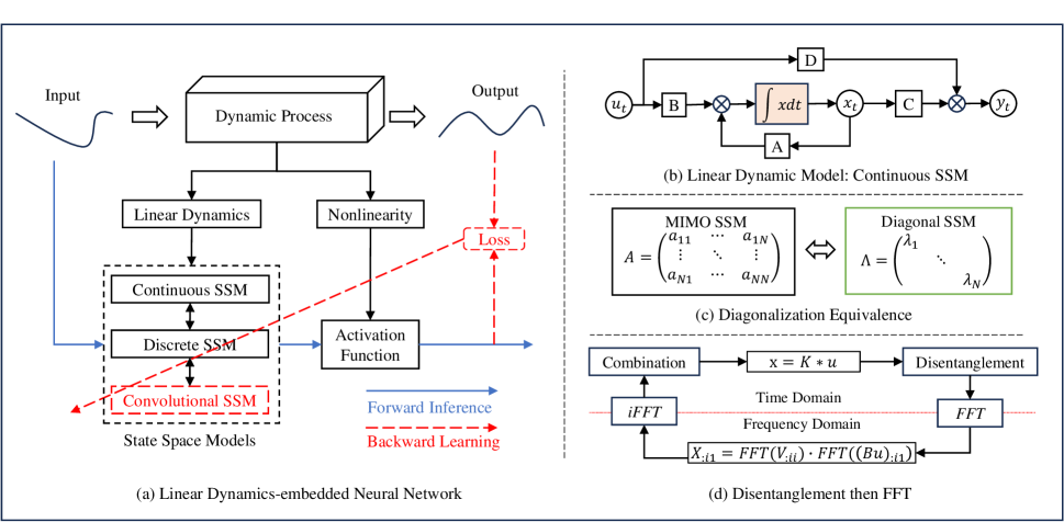
Figure 1: The Overall Framework of Linear Dynamics-embedded Neural Network (LDNN).

III-A Linear Dynamic Model

III-A1 Continuous SSMs

The continuous linear SSMs, as shown in Fig. 1 (b) are classical models to describe the dynamics of the linear systems. Typically, a continuous linear dynamic system with multi-input and multi-output (MIMO) is defined as the following general form:

$$\begin{cases}\dot{x}(t)=Ax(t)+Bu(t)\\ y(t)=Cx(t)+Du(t)\end{cases}$$ (2)

where system matrix $A\in\mathbb{R}^{N\times N}$, input matrix $B\in\mathbb{R}^{N\times H}$, output matrix $C\in\mathbb{R}^{M\times N}$, direct transition matrix $D\in\mathbb{R}^{M\times H}$. $u(t)\in\mathbb{R}^{H},x(t)\in\mathbb{R}^{N}$, and $y(t)\in\mathbb{R}^{M}$ are input, state, and output of the system.

In control theory, state $x$ is a variable that represents the dynamical state of the system. For example, when SSMs are used to model the moving process of an object, the state $x$ could include the velocity and acceleration of this object. However, in pure data cases, assigning the physical meanings for the state is intractable. We can understand this model from the perspective of polynomial projection. That is, given the sequence $\mathcal{U}$ generated from an unknown function $f$, $x$ are the coefficients of projected polynomials. Thus, $x$ can be seen as the compression of all history [13]. In other words, $x$ could be interpreted as the memory of history.

It should be noted that SSMs with single-input and single-output (SISO) are the special case of MIMO SSMs. Typically, the SISO SSMs, e.g., S4 [14] and DSS [15], are stacked in parallel and require an additional linear layer to mix features. However, MIMO SSMs model the multi-dimensional sequences directly, and no more feature-mixing layers are needed in theory.

III-A2 Discrete SSMs

We discrete the continuous SSMs (2) to learn from the discrete sequence. The discrete SSMs with a time step $\Delta\in\mathbb{R_{+}}$ are expressed as follows.

$$\begin{cases}x_{k}=\bar{A}x_{k-1}+\bar{B}u_{k}\\ y_{k}=\bar{C}x_{k}+\bar{D}u_{k}\end{cases}$$ (3)

There are many standard discretization technologies available. Coefficients matrix $\bar{C}=C$, and $\bar{D}=D$, but $\bar{A}$ and $\bar{B}$ would differ in different methods:
for the Zero-order Hold (ZOH) method [34],

$$\begin{cases}\bar{A}=e^{A\Delta}\\ \bar{B}=A^{-1}(e^{A\Delta}-I)B\end{cases}$$ (4)

for the Generalized Bilinear Transformation method (GBT).

$$\begin{cases}\bar{A}=(I-\alpha A\Delta)^{-1}(I+(1-\alpha)\Delta A)\\ \bar{B}=(I-\alpha\Delta A)^{-1}\Delta B\end{cases}$$ (5)

There are three special cases for the GBT with different $\alpha$: the forward Euler method is GBT with $\alpha=0$, the Bilinear method is GBT with $\alpha=0.5$, and the backward Euler method is GBT with $\alpha=1$. Those methods approximate the differential equation based on Taylor series expansion. More details about discretization methods are introduced in Appendix A.

Discrete SSMs are recurrent models, and state $x$ can be an analogy to the hidden state in RNNs. The recurrent models have excellent advantages in flexibility during the inference process but are hard to train.

III-A3 Convolutional SSMs

The convolution nature of SSMs makes it possible to train SSMs efficiently. Let the initial state be $x_{0}$, then unroll the recursive process Eq. (3) along time.

$$x_{1}=\bar{A}x_{0}+\bar{B}u_{1}$$

$$\vdots$$

$$x_{k}=\underbrace{\bar{A}^{k}x_{0}}_{bias}+\underbrace{\bar{A}^{k-1}\bar{B}u_{1}+\cdots+\bar{B}u_{k}}_{convolution\,operation}$$

$$\vdots$$

$$x_{L}=\bar{A}^{L}x_{0}+\bar{A}^{L-1}\bar{B}u_{1}+\cdots+\bar{B}u_{L}$$

From the above equations, we see that state $x_{i}$ is the summation of a bias and a convolution operation of all history inputs. For simplicity, we define the state kernel as Eq. (6).

$$K\triangleq\left(\bar{B},\bar{A}\bar{B},\cdots,\bar{A}^{i-1}\bar{B},\cdots,\bar{A}^{L-1}\bar{B}\right)$$ (6)

Then, the discrete SSMs (3) are reformulated into the convolutional representation of discrete SSMs Eq. (7). Besides, the convolutional view of continuous SSMs is given in Appendix B.

$$\begin{cases}x=K\ast u+Bias\\ y=\bar{C}x+\bar{D}u\end{cases}$$ (7)

where $u=\{u_{1},...,u_{L}\}$, $x=\{x_{1},...,x_{L}\}$, and $y=\{y_{1},...,y_{L}\}$ are discrete sequences sampled from continuous functions $u(t)$, $x(t)$, and $y(t)$.

The ground-true value of the initial state $x_{0}$ is unknown. Therefore, there is an error (the bias term $\bar{A}^{k}x_{0}$) between the estimated state $\hat{x}_{k}=K\ast u$ and ground-truth state $x_{k}$. Fortunately, based on Proposition 1, we can theoretically ignore the influence of the bias term.

Proposition 1 (State Convergence).

Let all eigenvalues of $A$ have a negative real part, for any given initial state $\hat{x}_{0}$, the estimated state $\hat{x}_{k}$ would convergent to their real values $x_{k}$.

Proof.

All eigenvalues of $A$ have negative real parts so we can get $0<\bar{A}<1$. Thus, the state converges as bias decays to 0 over time, i.e., $\lim_{k\to\infty}\left|x_{k}-\hat{x}_{k}\right|=\lim_{k\to\infty}\bar{A}^{k}x_{0}=0$. ∎

III-B Efficient Convolutional SSMs

Naively applying the convolutional SSMs (7) still has high time and space complexity. To break this computational bottleneck, we propose the following two strategies, see Fig. 1 (c) and (d).

III-B1 Uncouple SSMs via Diagonalization

The state kernel $K$ is the premise for the convolutional SSMs (7). We firstly rewrite the state kernel $K$ as $K=V\bar{B}$, where $V$ is the system kernel defined as follows.

$$V\triangleq\left(1,\bar{A},\cdots,\bar{A}^{i-1},\cdots,\bar{A}^{L-1}\right)$$ (8)

Calculating $V$ is extremely expensive if the system matrix $A$ is full. To solve this, we can uncouple the MIMO SSMs (2) into the diagonal SSMs (9) equivalently using the Diagonalization Equivalence Lemma.

lemma 1 (Diagonalization Equivalence).

Let matrix $A\in\mathbb{R}^{N\times N}$ has $N$ real and distinct eigenvalues {$\lambda_{1},...,\lambda_{N}$}, system (2) can be transformed equivalently into system (9) with $\Lambda=T^{-1}AT,B^{\prime}=T^{-1}B,C^{\prime}=CT,D^{\prime}=D$.

$$\begin{cases}\dot{z}(t)=\Lambda z(t)+B^{\prime}u(t)\\ y(t)=C^{\prime}z(t)+D^{\prime}u(t)\end{cases}$$ (9)

with $\Lambda=diag\{\lambda_{1},...,\lambda_{N}\}$.

Here, we omit the proof of Lemma 1, since it is similar to the proof of Theorem 11.1 in [35]. The diagonalization simplifies the calculation of $V$. Furthermore, the following statements that enable efficient calculation are derived:

• Given diagonal $\Lambda$, its discretization $\bar{\Lambda}$ is also diagonal.

• If using ZOH, $\bar{\Lambda}^{i}=diag\{e^{i\lambda_{1}\Delta},...,e^{i\lambda_{N}\Delta}\}$.

• The time complexity of $V$ is reduced from $O(LN^{3})$ to $O(LN)$.

• The space complexity of $V$ is reduced from $O(LN^{2})$ to $O(LN)$.

III-B2 Efficient convolution via FFT

Given $K$ and $u$, the convolution operation needs $O(L^{2}NH)$ multiplications, which are time-consuming and unable to be calculated in parallel. We propose a ^′Disentanglement then Fast Fourier Transform (FFT)^′ strategy to solve this problem.

Using $V$, we obtain Eq. (10). Then, we reformulate Eq. (10) into Eq. (11) based on the ${}^{\prime}\text{Associativity with Multiplication}^{\prime}$ property of convolution.

$$x =K\ast u$$

$$=VB\ast u$$ (10)

$$=V\ast Bu$$ (11)

It is well known that the convolution theorem realizes the efficient convolution calculation. More concretely, FFT could reduce the time complexity from $O(L^{2})$ to $O(L\log L)$ of convolution operation for a univariate polynomial [36].

However, the system kernel $V\in\mathbb{R}^{L\times N\times N}$ and projected input sequence $Bu\in\mathbb{R}^{L\times N\times 1}$ are multidimensional tensors. Thus, FFT cannot be used directly.

Based on the definition of convolution, we expand Eq. (11). For ease of understanding, we use the notation of tensor as introduced in [37]. The state at time $k$ is expressed as follows.

$$x_{k:1}=\sum_{m=1}^{k}V_{m::}\cdot(Bu)_{(k-m):1}$$ (12)

When we use diagonal SSMs, the system matrix $A$ becomes a diagonal matrix $\Lambda$. We simplify the previous equation and get Eq.(13).

$$x_{ki1}=\sum_{m=1}^{k}V_{mii}\cdot(Bu)_{(k-m)i1}$$ (13)

Using the definition of convolution, we reformulate Eq.(13) as

$$x_{:i1}=V_{:ii}\ast(Bu)_{:i1}$$ (14)

With this, we successfully disentangle the original convolution into Eq. (14), where $V_{:ii}$ and $(Bu)_{:i1}$ are both univariate sequence. We can apply FFT to calculate Eq. (14) efficiently.

$$x_{:i1}=iFFT\{FFT\{V_{:ii}\}\cdot FFT\{(Bu)_{:i1}\}\}$$ (15)

where $iFFT$ is the inverse FFT.

Proposition 2 (Efficient Convolution with Diagonalization).

Using diagonalization and ${}^{\prime}\text{Disentanglement then FFT}^{\prime}$ strategies, the convolution operation in Eq. (7) can be computed in reduced time complexity $O(LN\max\{H,\log L\})$ from $O(LNH\max\{L,N\})$.

Proof.

Given full matrix $A$ and $B$, we need $O(LN^{2}H)$ time complexity to obtain $K$. The convolution operation between $K$ and $u$ needs $O(L^{2}NH)$ time complexity. The overall time complexity is $O(LNH\max\{L,N\})$.

Using diagonalization and ${}^{\prime}\text{Disentanglement then FFT}^{\prime}$ strategies, we require $O(LNH)$ time complexity for the multiplication of $Bu$, and $O(LN)$ time complexity for $V$. Given $Bu$ and $V$, we need $O(LN\log{L})$ time complexity for Eq. (14). Thus, the overall time complexity is $O(LN\max\{H,\log L\})$. ∎

III-C Linear Dynamics-embedded Neural Network

The linear dynamic model together with activation function can serve as a new type of neural network. We call it Linear Dynamics-embedded Neural Network, abbreviated as LDNN. We further introduce more derails about LDNN in terms of initialization, causality, etc.

III-C1 Parameterization and Initialization of LDNN

The diagonal SSMs have learnable parameters $\Lambda,B^{\prime},C^{\prime},D^{\prime}$, and a time step $\Delta$ for discretization. We introduce the parameterization and initialization of these parameters, respectively.

Parameter $\Lambda$. According to Proposition 1, we know that all elements in $\Lambda$ must have negative real parts to ensure state convergence. Thus, we parameterize $\Lambda$ with an enforcing function $f_{+}$, expressed as $-f_{+}(Re(\Lambda))+Im(\Lambda)i$. The enforcing function $f_{+}$ outputs positive real numbers and may have many forms, for example, the Gaussian function, the rectified linear unit function (ReLU), and the Sigmoid function. A random or constant function can initialize $\Lambda$. Besides, it can be initialized by the eigenvalues of some specially structured matrices, such as the HiPPO matrix introduced in [13].

Parameter $B^{\prime}$ and $C^{\prime}$. $B^{\prime}$ and $C^{\prime}$ are the parameters of the linear projection function. We parameterize them as learnable full matrices. Furthermore, the initialization is given as random numbers or constant numbers.

Parameter $D^{\prime}$. Different parameterization of $D^{\prime}$ has different meanings. If we parameterize $D^{\prime}$ as an untrainable zero matrix, the output of SSMs is only dependent on the state. When the input and output are the same size, we can parameterize it as an identity matrix, also known as residual connection [38]. In addition, $D^{\prime}$ can be a trainable full matrix, which can be initialized as $B^{\prime}$ and $C^{\prime}$.

Parameter $\Delta$. $\Delta$ is a scalar for a given SSM. We set it as a learnable parameter and initialize it by randomly sampling from a bounded interval. This work uses [0.001, 0.1] as fault choice.

III-C2 Bidirectional non-causal LDNN

Proposition 3.

Linear SSMs are causal systems.

Proof.

The discrete SSMs are linear shift-invariant, and $K(t)=0$ if $t<0$. According to the definition of causal systems, linear SSMs are causal systems. ∎

As Proposition 3 says, the SSMs are causal models with a forward causal kernel $\overrightarrow{K}$, which only considers the historical and current sequences. Sometimes, we need to consider the whole sequence under a non-causal setting. Therefore, we propose the bidirectional non-causal LDNN by adding a backward kernel $\overleftarrow{K}$, which models reversal sequences. The state is calculated by the bidirectional state kernel $\overleftrightarrow{K}$ as described in Eq. (16) and Eq. (17).

We assume that the forward and backward processes have the same parameter $B$ but different $A$. Then, we reformulate Eq. (17) into Eq. (18) with forward system kernel $\overrightarrow{V}$ and backward system kernel $\overleftarrow{V}$. To sun up, the state calculation in the bidirectional LDNN is formulated as follows.

$$x =\overleftrightarrow{K}\ast u$$ (16)

$$=(\overrightarrow{K}+\overleftarrow{K})/2\ast u$$ (17)

$$=(\overrightarrow{V}+\overleftarrow{V})B/2\ast u$$ (18)

III-C3 Multi-Head LDNN

Following [7], we design the Multi-Head LDNN. Fig. 1 (d) illustrates the structure of Multi-Head LDNN. Multi-head LDNN use a ${}^{\prime}\text{divide and conque}^{\prime}$ intuition to construct multi-model for large-sized vectors in multiple subspaces. Specifically, the original input with a dimension of $H$ is first split into $h$ vectors of dimension $H/h$. Then, each split vector is modeled by the LDNN. The results of all LDNN are concatenated and linear projected as the output of Multi-Head LDNN.

$$\begin{split}\text{Multi-Head LDNN}(u)=&W\cdot Concat(LDNN_{1}(u_{1}),\\ &...,LDNN_{h}(u_{h}))+b\end{split}$$ (19)

where $W\in\mathbb{R}^{M\times N}$, and $b\in\mathbb{R}^{M}$.

The Multi-Head setting increases optionality and diversity in model selection but does not increase the total computational cost with the proper choice of $N,h$. This work found that $h=4$ is an appropriate choice for the default setting. Moreover, there is an extreme case where the original multivariate sequence is split into $H$ univariate sequences, i.e., $H=h$. In this case, the Multi-Head LDNN becomes stacked SISO SSMs, the base model in S4 and DSS.

IV Experiments

We measure the performance of the proposed LDNN on a wide range of sequence-level classification tasks, including audio, text, and images. Code and trained models to replicate the experiments can be found at: https://github.com/leonty1/DeepLDNN.

IV-A Experimental Setup

IV-A1 Dataset

Long Range Arena (LRA) [11] is a challenging and standard benchmark for evaluating the models’ long sequence classification performance. There are six tasks in LRA.

• LISTOPS [39]: It is a ten-way classification task containing a hierarchical structure and operators, and the sequence length is set as 2000.

• Text: The IMDB reviewers dataset [40] is processed and used for binary byte-level text classification with a sequence of 4000.

• Retrieval: This task measures the similarity between two sequence lengths 4000 based on the AAN dataset [41].

• Image: $32\times 32$ Images in CIFAR [42] are flattened into a sequence of length 1024 for classification tasks.

• Pathfinder [43]: The goal is to judge if two points are connected in a $32\times 32$ image. Images are flattened into a sequence of length 1024.

• PathX: It is an extreme case of Pathfinder with $128\times 128$ images.

IV-A2 Implementation

Following the basic setup in DSS [15], we implement our model with Pytorch [44] and use AdamW [45] as the optimizer. In the training process, we use cross entropy as the objective function for all classification tasks and use accuracy as evaluation metrics. We conduct all experiments on two NVIDIA RTX 3090 GPUs with 24 GB.

We discretize all continuous SSMs using ZOH. Some key hyperparameters of all our experiments are given in Table I. If not specified, learnable parameters are initialized from a standard random distribution. More details about the deep LDNN can be found in Appendix C.

TABLE I: Hyperparameters on LRA

Dataset	Batch	Epoch	n_layer	Head	H	N	M	LR			Dropout	A_ini	D	Activation	Bidirectional
								$\lambda$	$\Delta$	Others
ListOps	50	100	6	4	128	128	128	0.01	0.001	0.01	0	half	0	LeackyReLU	False
Text	64	60	4	2	128	128	128	0.01	0.001	0.01	0.1	half	1	LeackyReLU	False
Retrieval	64	40	4	4	64	64	64	0.01	0.001	0.01	0	half	1	LeackyReLU	False
Image	4	200	6	4	512	128	512	0.004	0.001	0.01	0.2	hippo	1	LeackyReLU	False
Pathfinder	100	200	6	4	256	128	256	0.004	0.001	0.01	0.1	half	1	LeackyReLU	False

IV-B Performance Comparison

We compare the results of our proposed model with nine baseline models. The nine models can show a diverse cross-section of long-sequence models.

• Transformer family: the standard vanilla Transformer [7]; three efficient variants, Reformer [46], Performer [28], and Luna-256 [47].

• F-net [48]: a FFT based attention-free model.

• CDIL-CNN [49]: a multi-scale model using Circular Dilated CNN.

• SSMs family: S4 [14], DSS [15], and S4D [16].

For a fair comparison, all results of baseline models are directly reused as reported in [11, 14, 49]. Then we compare our results with all baseline models in Table II.

Our model beats the Transformer family models and the F-net in almost all tasks. Furthermore, SSMs family modes, like S4 and DSS, are state-of-the-art (SOTA) models in LRA. The overall results present that our method achieves matchable performance with the SOTA models. Specifically, the LDNN is only 0.7% away from the best results (CDIL-CNN and DSS) in Listops. In Text, we obtain the second most accurate model behind the CDIL-CNN. Especially in Retrieval, we achieve the best performance, surpassing all baselines. Our model is also competitive with the most accurate models in Image, Pathfinder, and the average score. Unfortunately, the proposed LDNN fails to solve the extremely challenging Path-X task, as does the Transformer family, F-net, and the CDIL-CNN models. Overall, the results demonstrate the effectiveness and superiority of our proposed method.

TABLE II: Results on the LRA benchmark tasks

Model	ListOps	Text	Retrieval	Image	Pathfinder	Path-X	Avg.
length	2000	2048	4000	1024	1024	16384	-
Transformer	36.37	64.27	57.46	42.44	71.40	-	53.66
Reformer	37.27	56.10	53.40	38.07	68.50	-	50.56
Performer	18.01	65.40	53.82	42.77	77.05	-	51.18
Luna-256	37.25	64.57	79.29	47.38	77.72	-	59.37
FNet	35.33	65.11	59.61	38.67	77.80	-	54.42
CDIL-CNN	60.60	87.62	84.27	64.49	91.00	-	77.59
S4	58.35	76.02	87.09	87.26	86.05	88.10	80.48
DSS(softmax)	60.6	84.8	87.8	85.7	84.6	87.8	81.88
S4D	60.47	86.18	89.46	88.19	93.06	91.95	84.89
LDNN	59.90	87.31	90.19	85.33	85.47	-	81.64

IV-C Ablation Study

To better understand the LDNN, we conduct the following ablation studies.

IV-C1 On the Initialization of $\Lambda$

We experimentally investigate the effect of different initialization strategies of diagonal system matrix $\Lambda$ on the model’s performance. We use a randomly generated matrix, the HiPPO matrix, and a constant matrix with all diagonal values of 1/2, abbreviated as ${}^{\prime}\text{randn}^{\prime}$, ${}^{\prime}\text{hippo}^{\prime}$, and ${}^{\prime}\text{half}^{\prime}$, respectively. We visualize the testing accuracy after each training epoch in Fig. 2 and Fig. 3.

In Fig. 2, the solid lines are the results of models trained with a learning rate of 0.001 for $\Lambda$ on ListOps. The ${}^{\prime}\text{randn}^{\prime}$ and ${}^{\prime}\text{hippo}^{\prime}$ achieve similar accuracy, but ${}^{\prime}\text{half}^{\prime}$ has the worst result. To further explore the reason for ${}^{\prime}\text{half}^{\prime}$s behavior, we increase the learning rate of $\Lambda$ to 0.01. As shown with the dotted red line (${}^{\prime}\text{hippo-1}^{\prime}$) in Fig. 2, the model obtains high accuracy as other initialization strategies.

A similar phenomenon can also be found in the IMDB dataset. The accuracy of ${}^{\prime}\text{hippo}^{\prime}$ is lower than ${}^{\prime}\text{randn}^{\prime}$ and ${}^{\prime}\text{half}^{\prime}$ with a learning rate of 0.01. However, a more accurate result can be obtained if we set the learning rate as 0.001 for initialization with ${}^{\prime}\text{hippo}^{\prime}$. See the dotted red line ${}^{\prime}\text{hippo-1}^{\prime}$ in Fig. 3.

Therefore, the results suggest that different initialization strategies, if given a proper learning rate, can produce high accuracy, which is different from the findings in [16].

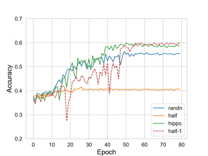
Figure 2: Testing Accuracy with Different Initialization of $\Lambda$ on ListOps.

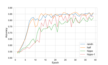
Figure 3: Testing Accuracy with Different Initialization of $\Lambda$ on IMDB.

IV-C2 On the Parameterization of $D^{\prime}$

We conduct an ablation study on the parameterization of $D^{\prime}$ in four tasks. We keep all hyperparameters the same in each experiment except $D^{\prime}$. We parameterize $D^{\prime}$ in three ways as introduced in Section III-C1. Table III shows that different parameterizations of $D^{\prime}$ will affect the model’s accuracy. Models with $D^{\prime}$ as zero matrices achieve the best results in ListOps and Text. Parameterizing $D^{\prime}$ as an identity matrix obtains the highest accuracy in Retrieval and Image. Therefore, different parameterizations of $D^{\prime}$ result in different accuracy, and we must carefully set the parameter $D^{\prime}$ for the specific database.

TABLE III: Ablation Studies on Different Hyperparameters

Dataset	$D^{\prime}$			Head			Bidirectional
	Zero	Identity	Full	2	4	8	False	True
ListOps	58.95	58.85	56.85	40.95	59.90	53.50	-	-
Text	86.60	86.52	86.55	87.31	85.89	86.14	86.52	85.41
Retrieval	89.55	90.19	89.23	89.65	90.19	-	90.19	89.94
Image	83.40	85.33	84.98	83.48	85.33	84.37	85.33	82.14

IV-C3 On the Multi-Head LDNN

The number of heads is set to 2, 4, and 8 for ablation experiments. In Table III, ${}^{\prime}-^{\prime}$ denotes the corresponding experiment is not conducted. The results show that model with 2 heads has the best result in Text, and models with 4 heads are best in ListOps, Retrieval, and Image. Therefore, an appropriate choice of the number of heads can obtain a model with better performance. We recommend setting the number of heads to 4 as the default value.

IV-C4 On the Bidirectional LDNN

We conduct an ablation study on the bidirectional setting of the system kernel on three non-causal tasks. Unfortunately, models with the bidirectional kernel do not perform better in the experiments as presented in Table III. Even so, the directional setting, on the one hand, improves the model at the theoretical level and, on the other hand, provides a variety of options for model selection in different tasks.

V Conclusion

This work proposes a new type of neural network for long-sequence modeling called Linear Dynamics Embedded Neural Network (LDNN). The proposed LDNN are designed based on state space models with multi-input and muti-output, thus having a solid theoretical foundation. Besides, the LDNN can be trained efficiently in convolutional representation with the help of diagonalization and ^′Disentanglement then Fast Fourier Transform (FFT)^′ strategies. Furthermore, the multi-head and bidirectional settings improve the diversity and flexibility of the models, enabling them to be applied to various cases and tasks. We stack the LDNN as a deep model on extensive experiments. The results validate that the LDNN have matchable state-of-the-art performance in Long Range Arena (LRA). We hope this work can provide an efficient solution for modeling long sequences and provide potential directions for the theoretical design of neural networks via combining control theory.

Appendix A Numerical Discretization

A-A Zero-order Hold Method

The state transition function is an ordinary differential equation (ODE). We can reformulate it as follows.

$$\dot{x}(t)=Ax(t)+Bu(t)$$

$$\dot{x}(t)-Ax(t)=Bu(t)$$

$$e^{-tA}\dot{x}(t)-e^{-tA}Ax(t)=e^{-tA}Bu(t)$$

$$\frac{1}{dt}\left[e^{-tA}x(t))\right]=e^{-tA}Bu(t)$$

$$\int_{0}^{t}\frac{1}{d\tau}\left[e^{-\tau A}x(\tau)\right]d\tau=\int_{0}^{t}e^{-\tau A}Bu(\tau)d\tau$$

$$e^{-tA}x(t)-x(0)=\int_{0}^{t}e^{-\tau A}Bu(\tau)d\tau$$

$$x(t)=e^{tA}x(0)+e^{tA}\int_{0}^{t}e^{-\tau A}Bu(\tau)d\tau$$

$$x(t)=e^{At}x(0)+\int_{0}^{t}e^{A(t-\tau)}Bu(\tau)d\tau$$ (A.20)

Eq. (A.20) is the analytical solution of $x(t)$. Then, we rewrite Eq. (A.20) with initial time $t_{0}$.

$$x(t)=e^{A(t-t_{0})}x(t_{0})+\int_{t_{0}}^{t}e^{A(t-\tau)}Bu(\tau)d\tau$$ (A.21)

When we sample the $u(t)$ with time interval $\Delta$, $t$ becomes $k\Delta$ where $k=0,1,...$ is a positive integer. The Zero-order Hold method assumes that $u(t)=u(k\Delta)$. For $t\in[k\Delta,(k+1)\Delta]$. Thus, we have

$$x((k+1)\Delta)=e^{A(\Delta)}x(k\Delta)+\int_{k\Delta}^{(k+1)\Delta}e^{A((k+1)\Delta-\tau)}d\tau Bu(k\Delta)$$ (A.22)

We abbreviate $x((k+1)\Delta)$, $x(k\Delta)$, and $u(k\Delta)$ as $x_{k+1}$, $x_{k}$, and $u_{k}$, respectively. Here, we get the discrete transition function.

$$x_{k+1}=\bar{A}x_{k}+\bar{B}u_{k}$$ (A.23)

with $\bar{A}=e^{A\Delta}$, $\bar{B}=\int_{k\Delta}^{(k+1)\Delta}e^{A((k+1)\Delta-\tau)}d\tau B$.

We can further simplify $\bar{B}$ assuming that $A$ is invertible.

$$\bar{B} =\int_{k\Delta}^{(k+1)\Delta}e^{A((k+1)\Delta-\tau)}d\tau B$$

$$=\int_{0}^{\Delta}e^{At}dtB$$

$$=\int_{0}^{\Delta}A^{-1}\frac{de^{At}}{dt}dtB$$

$$=A^{-1}(e^{At}-I)B$$ (A.24)

A-B Numerical Approximation

Based on Taylor series expansion, the first derivative of $x$ can be approximated by numerical differentiation. Using the forward Euler Eq. (A.25), or the backward Euler Eq. (A.26) to approximate ${x}$, we obtain the $\bar{A}$, and $\bar{B}$ as described in Eq. (5).

$$\frac{x_{k+1}-x_{k}}{\Delta}\approx\dot{x}_{k}=Ax_{t}+Bu_{t}$$ (A.25)

$$\frac{x_{k+1}-x_{k}}{\Delta}\approx\dot{x}=Ax_{t+1}+Bu_{t}$$ (A.26)

Appendix B Convolutional View of continuous SSMs

Here, we introduce the convolutional view of continuous SSMs [50].

$$x(t) =e^{At}x(0)+\int_{0}^{t}e^{A(t-\tau)}Bu(\tau)d\tau$$

$$=e^{At}x(0)+\int_{0}^{t}e^{At}Bu(t-\tau)d\tau$$ (B.27)

$$=e^{At}x(0)+\int_{0}^{t}h(t)u(t-\tau)d\tau$$ (B.28)

$$=e^{At}x(0)+(h\ast u)(t)$$ (B.29)

Using the change of variables, we reformulate Eq. (B.27). Let $h(t)=e^{At}B$, we obtain the convolutional SSMs (B.29) based on the definition of convolution.

Appendix C Model Details

C-A Initialization with HiPPO Matrix

Following DSS [15], we use the eigenvalues of the following HiPPO matrix as the initialization of diagonal matrix $\Lambda$.

$$\begin{cases}(2i+1)^{1/2}(2j+1)^{1/2}/2&i<j\\ -1/2&i=j\\ -(2i+1)^{1/2}(2j+1)^{1/2}/2&i>j\end{cases}$$ (C.30)

C-B Deep Model Architecture

In the experiments, we use the Multi-Head LDNN, Fig. 4 (a), as the basic linear layer to construct the deep model. A LeakyReLU activation function is applied to increase the nonlinear ability of the deep model. In addition, there is a residual connection between the Multi-Head LDNN input and the activation function output. We add (layer or batch) normalization at the end of each module.

The input sequence with length $L$ is first transformed into a sequence with a $(H,L)$ shape. Then, the proposed LDNN, stacked into a deep structure (Fig. 4 (b)), takes the encoded sequence as input and outputs a sequence with the shape of $(M,L)$. Eventually, the decoder transforms the output sequence into a vector for classification. The encoder and decoder are embedding layers or linear projections implemented by the linear layer.

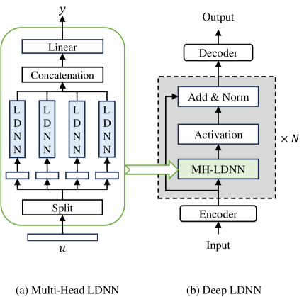
Figure 4: Deep Model Architecture.

Tongyi Liang received the B.E. degree in automotive engineering from the University of Science and Technology Beijing, Beijing, China, in 2017, the M.E. degree in automotive engineering from the Beihang University, Beijing, China, in 2020. He is currently working toward the Ph.D degree with the Department of Systems Engineering, City University of Hong Kong, Hong Kong, China. His current research interests focus on machine learning and neural networks.

Han-Xiong Li (Fellow, IEEE) received the B.E. degree in aerospace engineering from the National University of Defense Technology, Changsha, China, in 1982, the M.E. degree in electrical engineering from the Delft University of Technology, Delft, The Netherlands, in 1991, and the Ph.D. degree in electrical engineering from the University of Auckland, Auckland, New Zealand, in 1997. He is the Chair Professor with the Department of Systems Engineering, City University of Hong Kong, Hong Kong. He has a broad experience in both academia and industry. He has authored two books and about 20 patents, and authored or coauthored more than 250 SCI journal papers with h-index 52 (web of science). His current research interests include process modeling and control, distributed parameter systems, and system intelligence. Dr. Li is currently the Associate Editor for IEEE Transactions on SMC: System and was an Associate Editor for IEEE Transactions on Cybernetics (2002-–2016) and IEEE Transactions on Industrial Electronics (2009–-2015). He was the recipient of the Distinguished Young Scholar (overseas) by the China National Science Foundation in 2004, Chang Jiang Professorship by the Ministry of Education, China in 2006, and National Professorship with China Thousand Talents Program in 2010. Since 2014, he has been rated as a highly cited scholar in China by Elsevier.

References

- [1] K. Chowdhary and K. Chowdhary, “Natural language processing,” Fundamentals of artificial intelligence, pp. 603–649, 2020.
- [2] D. Bautista and R. Atienza, “Scene text recognition with permuted autoregressive sequence models,” in European Conference on Computer Vision. Springer, 2022, pp. 178–196.
- [3] F. Petropoulos, D. Apiletti, V. Assimakopoulos, M. Z. Babai, D. K. Barrow, S. B. Taieb, C. Bergmeir, R. J. Bessa, J. Bijak, J. E. Boylan et al., “Forecasting: theory and practice,” International Journal of Forecasting, vol. 38, no. 3, pp. 705–871, 2022.
- [4] Y. Bengio, N. Boulanger-Lewandowski, and R. Pascanu, “Advances in optimizing recurrent networks,” in 2013 IEEE international conference on acoustics, speech and signal processing. IEEE, 2013, pp. 8624–8628.
- [5] S. Hochreiter and J. Schmidhuber, “Long short-term memory,” Neural computation, vol. 9, no. 8, pp. 1735–1780, 1997.
- [6] M. Schuster and K. K. Paliwal, “Bidirectional recurrent neural networks,” IEEE transactions on Signal Processing, vol. 45, no. 11, pp. 2673–2681, 1997.
- [7] A. Vaswani, N. Shazeer, N. Parmar, J. Uszkoreit, L. Jones, A. N. Gomez, Ł. Kaiser, and I. Polosukhin, “Attention is all you need,” Advances in neural information processing systems, vol. 30, 2017.
- [8] Y. Liu, Y. Zhang, Y. Wang, F. Hou, J. Yuan, J. Tian, Y. Zhang, Z. Shi, J. Fan, and Z. He, “A survey of visual transformers,” IEEE Transactions on Neural Networks and Learning Systems, 2023.
- [9] H. Zhou, S. Zhang, J. Peng, S. Zhang, J. Li, H. Xiong, and W. Zhang, “Informer: Beyond efficient transformer for long sequence time-series forecasting,” in Proceedings of the AAAI conference on artificial intelligence, vol. 35, no. 12, 2021, pp. 11 106–11 115.
- [10] Y. Zhang and J. Yan, “Crossformer: Transformer utilizing cross-dimension dependency for multivariate time series forecasting,” in The Eleventh International Conference on Learning Representations, 2022.
- [11] Y. Tay, M. Dehghani, S. Abnar, Y. Shen, D. Bahri, P. Pham, J. Rao, L. Yang, S. Ruder, and D. Metzler, “Long range arena: A benchmark for efficient transformers,” arXiv preprint arXiv:2011.04006, 2020.
- [12] A. Gu, I. Johnson, K. Goel, K. Saab, T. Dao, A. Rudra, and C. Ré, “Combining recurrent, convolutional, and continuous-time models with linear state space layers,” Advances in neural information processing systems, vol. 34, pp. 572–585, 2021.
- [13] A. Gu, T. Dao, S. Ermon, A. Rudra, and C. Ré, “Hippo: Recurrent memory with optimal polynomial projections,” Advances in neural information processing systems, vol. 33, pp. 1474–1487, 2020.
- [14] A. Gu, K. Goel, and C. Ré, “Efficiently modeling long sequences with structured state spaces,” arXiv preprint arXiv:2111.00396, 2021.
- [15] A. Gupta, A. Gu, and J. Berant, “Diagonal state spaces are as effective as structured state spaces,” Advances in Neural Information Processing Systems, vol. 35, pp. 22 982–22 994, 2022.
- [16] A. Gu, K. Goel, A. Gupta, and C. Ré, “On the parameterization and initialization of diagonal state space models,” Advances in Neural Information Processing Systems, vol. 35, pp. 35 971–35 983, 2022.
- [17] C. Li, Z. Zhang, W. S. Lee, and G. H. Lee, “Convolutional sequence to sequence model for human dynamics,” in Proceedings of the IEEE conference on computer vision and pattern recognition, 2018, pp. 5226–5234.
- [18] D. W. Romero, A. Kuzina, E. J. Bekkers, J. M. Tomczak, and M. Hoogendoorn, “Ckconv: Continuous kernel convolution for sequential data,” arXiv preprint arXiv:2102.02611, 2021.
- [19] Y. Li, T. Cai, Y. Zhang, D. Chen, and D. Dey, “What makes convolutional models great on long sequence modeling?” arXiv preprint arXiv:2210.09298, 2022.
- [20] D. Y. Fu, E. L. Epstein, E. Nguyen, A. W. Thomas, M. Zhang, T. Dao, A. Rudra, and C. Ré, “Simple hardware-efficient long convolutions for sequence modeling,” arXiv preprint arXiv:2302.06646, 2023.
- [21] A. Voelker, I. Kajić, and C. Eliasmith, “Legendre memory units: Continuous-time representation in recurrent neural networks,” Advances in neural information processing systems, vol. 32, 2019.
- [22] R. T. Chen, Y. Rubanova, J. Bettencourt, and D. K. Duvenaud, “Neural ordinary differential equations,” Advances in neural information processing systems, vol. 31, 2018.
- [23] Y. Rubanova, R. T. Chen, and D. K. Duvenaud, “Latent ordinary differential equations for irregularly-sampled time series,” Advances in neural information processing systems, vol. 32, 2019.
- [24] P. Kidger, J. Morrill, J. Foster, and T. Lyons, “Neural controlled differential equations for irregular time series,” Advances in Neural Information Processing Systems, vol. 33, pp. 6696–6707, 2020.
- [25] I. Beltagy, M. E. Peters, and A. Cohan, “Longformer: The long-document transformer,” arXiv preprint arXiv:2004.05150, 2020.
- [26] M. Zaheer, G. Guruganesh, K. A. Dubey, J. Ainslie, C. Alberti, S. Ontanon, P. Pham, A. Ravula, Q. Wang, L. Yang et al., “Big bird: Transformers for longer sequences,” Advances in neural information processing systems, vol. 33, pp. 17 283–17 297, 2020.
- [27] R. Child, S. Gray, A. Radford, and I. Sutskever, “Generating long sequences with sparse transformers,” arXiv preprint arXiv:1904.10509, 2019.
- [28] K. Choromanski, V. Likhosherstov, D. Dohan, X. Song, A. Gane, T. Sarlos, P. Hawkins, J. Davis, A. Mohiuddin, L. Kaiser et al., “Rethinking attention with performers,” arXiv preprint arXiv:2009.14794, 2020.
- [29] A. Katharopoulos, A. Vyas, N. Pappas, and F. Fleuret, “Transformers are rnns: Fast autoregressive transformers with linear attention,” in International conference on machine learning. PMLR, 2020, pp. 5156–5165.
- [30] A. Vyas, A. Katharopoulos, and F. Fleuret, “Fast transformers with clustered attention,” Advances in Neural Information Processing Systems, vol. 33, pp. 21 665–21 674, 2020.
- [31] Q. Guo, X. Qiu, X. Xue, and Z. Zhang, “Low-rank and locality constrained self-attention for sequence modeling,” IEEE/ACM Transactions on Audio, Speech, and Language Processing, vol. 27, no. 12, pp. 2213–2222, 2019.
- [32] H. Mehta, A. Gupta, A. Cutkosky, and B. Neyshabur, “Long range language modeling via gated state spaces,” arXiv preprint arXiv:2206.13947, 2022.
- [33] J. T. Smith, A. Warrington, and S. W. Linderman, “Simplified state space layers for sequence modeling,” arXiv preprint arXiv:2208.04933, 2022.
- [34] G. Gu, Discrete-time linear systems: theory and design with applications. Springer Science & Business Media, 2012.
- [35] J. Lu, “Matrix decomposition and applications,” arXiv preprint arXiv:2201.00145, 2022.
- [36] K. R. Rao, D. N. Kim, and J. J. Hwang, Fast Fourier transform: algorithms and applications. Springer, 2010, vol. 32.
- [37] T. G. Kolda and B. W. Bader, “Tensor decompositions and applications,” SIAM review, vol. 51, no. 3, pp. 455–500, 2009.
- [38] K. He, X. Zhang, S. Ren, and J. Sun, “Deep residual learning for image recognition,” in Proceedings of the IEEE conference on computer vision and pattern recognition, 2016, pp. 770–778.
- [39] N. Nangia and S. R. Bowman, “Listops: A diagnostic dataset for latent tree learning,” arXiv preprint arXiv:1804.06028, 2018.
- [40] A. Maas, R. E. Daly, P. T. Pham, D. Huang, A. Y. Ng, and C. Potts, “Learning word vectors for sentiment analysis,” in Proceedings of the 49th annual meeting of the association for computational linguistics: Human language technologies, 2011, pp. 142–150.
- [41] D. R. Radev, P. Muthukrishnan, V. Qazvinian, and A. Abu-Jbara, “The acl anthology network corpus,” Language Resources and Evaluation, vol. 47, pp. 919–944, 2013.
- [42] A. Krizhevsky, G. Hinton et al., “Learning multiple layers of features from tiny images,” 2009.
- [43] D. Linsley, J. Kim, V. Veerabadran, C. Windolf, and T. Serre, “Learning long-range spatial dependencies with horizontal gated recurrent units,” Advances in neural information processing systems, vol. 31, 2018.
- [44] A. Paszke, S. Gross, F. Massa, A. Lerer, J. Bradbury, G. Chanan, T. Killeen, Z. Lin, N. Gimelshein, L. Antiga et al., “Pytorch: An imperative style, high-performance deep learning library,” Advances in neural information processing systems, vol. 32, 2019.
- [45] I. Loshchilov and F. Hutter, “Decoupled weight decay regularization,” arXiv preprint arXiv:1711.05101, 2017.
- [46] N. Kitaev, Ł. Kaiser, and A. Levskaya, “Reformer: The efficient transformer,” arXiv preprint arXiv:2001.04451, 2020.
- [47] X. Ma, X. Kong, S. Wang, C. Zhou, J. May, H. Ma, and L. Zettlemoyer, “Luna: Linear unified nested attention,” Advances in Neural Information Processing Systems, vol. 34, pp. 2441–2453, 2021.
- [48] J. Lee-Thorp, J. Ainslie, I. Eckstein, and S. Ontanon, “Fnet: Mixing tokens with fourier transforms,” arXiv preprint arXiv:2105.03824, 2021.
- [49] L. Cheng, R. Khalitov, T. Yu, J. Zhang, and Z. Yang, “Classification of long sequential data using circular dilated convolutional neural networks,” Neurocomputing, vol. 518, pp. 50–59, 2023.
- [50] H. Hè and M. Kabic, “A unified view of long-sequence models towards million-scale dependencies,” arXiv preprint arXiv:2302.06218, 2023.