Fractional phase jumps in stochastic systems with tilted periodic double-well potentials

Abstract

We present a theoretical investigation of the stochastic dynamics of a damped particle in a tilted periodic potential with a double well per period. By applying the matrix continued fraction technique to the Fokker-Planck equation in conjunction with the full counting statistics and master equation approaches, we determine the rates of specific processes contributing to the system’s overall dynamics. At low temperatures, the system can exhibit one running state and two distinct locked metastable states. We focus primarily on two aspects: the dynamics of phase jumps, which are rare thermally induced particle jumps over potential maxima, and their impact on the overall velocity noise; and the retrapping process, involving the transition from the running to the locked metastable states. We demonstrate the existence of fractional (in units of $2\pi$) phase slips that differ qualitatively from conventional $2\pi$ jumps observed in single-well systems. Fractional phase slips significantly influence the system dynamics even in regimes dominated by dichotomous-like switching between running and locked states. Furthermore, we introduce a simple master equation approach that proves effective in analyzing various stages of the retrapping process. Interestingly, our analysis shows that even for a system featuring a well-developed double-well periodic potential, there exists a broad parameter range where the stochastic dynamics can be accurately described by an effective single-well periodic model. The techniques introduced here allow for valuable insights into the complex behavior of the system, offering avenues for understanding and controlling its steady-state and transient dynamics, which go beyond or can be complementary to direct stochastic simulations.

I Introduction

The stochastic dynamic motion of a particle in tilted periodic potentials plays an important role in the studies of various physical phenomena including Josephson junctions (JJs) [1, 2, 3, 4, 5], microparticles confined in shaped laser beams [6, 7, 8, 9, 10, 11, 12, 13], dynamics of charge density waves [14], crystal surface melting [15, 16], ratchet and molecular motors [17, 18, 19], cold atoms in optical lattices [20], different bio-physical processes [21] as well as in investigations of phenomena such as anomalous diffusion and memory effects [22, 23, 24, 25, 26]. A well-paid effort has already been invested in the theoretical analysis of such systems [27, 28, 29, 30], yet there are still plenty of open questions often inspired by the recent experimental realizations in different systems, e.g., Refs. [4, 13, 31, 32]. Moreover, experimental progress in different fields called for readdressing some old problems such as escape and retrapping of the Brownian particle from or to potential minima [33, 34, 35, 36, 37, 24], the statistics of thermally activated jumps of the particle by integer multiples of $2\pi$ (i.e., phase jumps) [38, 39, 40, 35] and multistability [24, 41, 42].

In this respect, of special interest are systems where the stochastic dynamics of the particle is affected by a biharmonic potential containing two local minima per period

$$U(\varphi) = -\varphi\,i_{b}+U_{0}(\varphi),$$ (1)

$$U_{0}(\varphi) = -\alpha\cos\varphi+\frac{1}{2}\cos 2\varphi,$$

where $i_{b}$ is a static external bias force, i.e., a potential tilt, $U_{0}(\varphi)$ is the untilted periodic double-well potential, where the coefficient $\alpha$ tunes the ratio of the first to the second harmonic contribution and $\varphi=2\pi x/\lambda$, where $x$ is the coordinate (position) and $\lambda$ the period. Consistent with papers focusing, for example, on the Josephson junctions, we call the variable $\varphi$ phase. The potential (1) plays an important role in the theoretical description of numerous physical systems, including JJs with substantial second harmonic in the current phase relation (CPR) [43, 44, 45, 46, 47, 48, 49, 50, 51, 52, 53, 54, 4, 55, 56] in particular in Josephson diodes [57, 58, 31] or various ratchet systems [59, 60, 61] and molecular motors [62, 63].

A careful analysis of the motion of the particle in the tilted double-well potential has already led to some important results. For example, it explained the existence of two critical escape currents from the superconducting to the resistive state observed experimentally for the JJs with doubly degenerate ground state (i.e., $\varphi$-Junctions) [48], pointed to rather nontrivial retrapping dependencies of the phase which can lead to a butterfly effect [50] and showed the existence of chaotic phase trajectories in various generalizations of the famous RCSJ model [64, 65]. The case $\alpha=0$, where only the second harmonic is present in the potential, plays an important role in the studies of unconventional junctions which can undergo the so-called $0$-$\pi$ transition [66, 54]. Moreover, a Brownian particle moving in the potential (1) with additional harmonic terms, characterized by asymmetric mobility considering bias force, is an archetypal model of the ratchet and diode systems [59, 61, 57, 58].

A crucial component in all of the above phenomena is noise. In combination with different dampings, a system with potential (1) can show a wide variety of regimes, each important for different physical realizations. Here, we provide a systematic analysis of a general case. We start with the simple strong damping parameter regime and proceed to the more complicated intermediate and weak damping regimes. We use velocity-noise to identify three main dynamic regimes [35]: the thermal noise regime; the phase-jumps (PJs) regime, and the switching regime. In each, we focus on the analysis of the dominant dynamics. In particular, we investigate the statistics of the phase jumps and their contribution to the overall velocity noise in the PJs regime and the escape and retrapping processes in the switching one. For this purpose, we combine the matrix continued-fraction (MCF) method with other techniques. In particular, in Sec. II we introduce a combination of the matrix continued-fraction (MCF) technique [27] with full counting statistics (FCS) [67, 68, 69] for the analysis of the multiple PJs. Its biggest advantage over the stochastic simulations is that it is straightforward to access the steady state. As such, it is suitable for the calculation of rates for rare events. Therefore, in the relevant regime, this method allows decomposition of the phase dynamics into independent elementary processes [70, 71, 72], constituted by single or multiple phase jumps. Using this method, we demonstrate the existence of the so-called fractional PJ in Sec. III.2.1. In Sec. III.2.2 we investigate retrapping processes in the switching regime. Here we combine the MCF with an effective master equation approach describing the transition of the system between its three metastable regimes. On top of the steady-state studies, we also discuss in Sec. III.2.3 a dynamical retrapping scenario.

There is a particular conclusion of our research that is worth foreshadowing here. Namely, for a broad range of parameters, even a system with a well-developed double-well potential can be faithfully described by a single-well model.

II Model and Methods

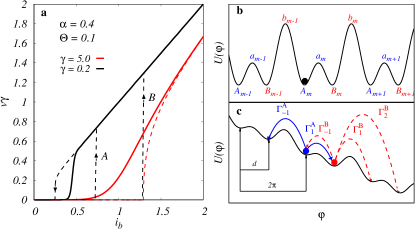
Figure 1: (a) Examples of $v-i_{b}$ characteristics representing the strong damping ($\gamma=5$ plotted with red lines) and the weak damping regime ($\gamma=0.2$ plotted with black lines). The thin dashed lines show the deterministic (noise-free) solutions. The solid thick lines represent stationary solutions for temperature $\Theta=0.1$. (b) -(c) Illustrations of the potential Eq. (1) with $\Gamma^{A}_{n}$ and $\Gamma^{B}_{n}$ being the rates of the forward / backward phase jumps over $n$ local maxima. In general the distance $d$ is not equal to $\pi$.

II.1 Model and dynamical regimes

We consider a stochastic motion of a particle in a potential $U(\varphi)$ described by the dimensionless Langevine equations

$$\begin{split}\frac{\partial v(\tau)}{\partial\tau}&=-\gamma v(\tau)-\frac{\partial U(\varphi)}{\partial\varphi}+\zeta(\tau),\\ v(\tau)&=\partial\varphi/\partial\tau,\end{split}$$ (2)

where $v$ is the velocity of the particle, $\gamma$ is the friction coefficient and $\zeta$ represents a Gaussian white noise with the zero mean $\langle\zeta(\tau)\rangle=0$ and correlation function $\langle\zeta(\tau_{1})\zeta(\tau_{2})\rangle=2\gamma\Theta\delta(\tau_{1}-\tau_{2})$ where $\Theta$ is the dimensionless temperature. The associated Fokker-Planck equation [27] of Eqs. (2) for the probability distribution function $W(\varphi,v,\tau)$ in the case of potential (1) reads

$$\dfrac{\partial}{\partial\tau}W(\varphi,v;\tau) = \dfrac{\partial}{\partial v}\left(\gamma v+\alpha\sin\varphi-\sin 2\varphi-i_{b}\right)W$$

$$-v\dfrac{\partial}{\partial\varphi}W+\gamma\Theta\dfrac{\partial^{2}}{\partial v^{2}}W$$

$$\equiv L_{\mathrm{FP}}W(\varphi,v;\tau).$$

The derivation of the average velocity

$$\langle v\rangle=\int\limits_{0}^{2\pi}\mathrm{d}\varphi\int\limits_{-\infty}^{\infty}\mathrm{d}vvW_{\mathrm{stat}}(\varphi,v)$$ (4)

follows closely the standard MCF method [27, Sec. 11.5] and the derivation of (zero-frequency) velocity noise

$$S=\int\limits_{-\infty}^{\infty}\mathrm{d}\tau\big{(}\langle v(\tau)v(0)\rangle-\langle v(\tau)\rangle\langle v(0)\rangle\big{)}$$ (5)

in the stationary state $W_{\mathrm{stat}}(\varphi,v)\equiv\lim_{\tau\to\infty}W(\varphi,v;\tau)$ follows that of Ref. [35].

Figs. 1(b)-(c) illustrate the system for zero and finite bias force. The potential (1) has for $\alpha<2$ and zero bias two types of minima marked as $A$ and $B$ and two types of maxima ($a$ and $b$). Consequently, there are also two critical bias forces: $i_{cA}$ where the minimum $A$ and maximum $a$ disappear and $i_{cB}$ where the minimum $B$ and maximum $b$ disappear. The system can be in three distinct stationary regimes. Namely, the particle can be running, i.e., at high bias force, or it can be locked in one of the potential minima types. Consequently, for the noiseless case, the initial position of the particle can, depending on the damping, play an important role even for the steady state, as illustrated in Fig. 1(a).

To explain this, let us consider two limiting cases, one with a strong damping and the other with a weak damping. In both cases, first slowly (compared to any other process) ramp the bias force from $i_{b}=0$ to $i_{cB}$ with the aim of observing the escape of the particle from a potential well. Afterwards, we assume a backward ramping from $i_{b}\gg i_{cB}$ to $i_{b}=0$ with the aim of observing the recapture (retrapping) of the running particle in one of the wells.

For strong damping [$\gamma=5$ in Fig. 1(a)] there is only a single escape bias force and it is identical to the retrapping force. Due to the strong damping, the initial position of the trapped particle does not play a role in this regime. The particle will start running only after the higher maximum $b$ disappears and, vice versa, will be retrapped at the minimal bias force for which the maximum $b$ appears. Therefore, both the critical escape force and the retrapping force are equal to $i_{cB}$ (red dashed line).

In contrast, there are two possible escape tilts for weak damping ($\gamma=0.2$). If the particle initially is trapped at the minimum $A$, it will obtain enough inertia to overcome the still existing maximum $b$ already at the first critical force $i_{cA}$. However, if it is initially trapped at the minimum $B$ it will stay there until the second critical force $i_{cB}$ is reached. The retrapping is also more complicated than in the strong-damping case. If the particle is already running, then it has enough inertia to overcome the local maxima existing below the critical force $i_{cB}$ or even $i_{cA}$ up to the actual retrapping force $i_{r}$ [73], black dashed lines in Fig. 1(a). The retrapping force is determined by the energy balance between the energy supply of the bias force and the dissipation [27, 50]. This means that there is a region of coexistence of the running and the locked state solutions. The question in which minimum will the particle be trapped requires careful analysis because it is a parameter-sensitive process which can lead to a deterministic butterfly effect [50, 74].

The noise makes the dynamics even more complicated. Additional processes, such as switching between running and locked states or occasional jumps of the particle over the neighboring maxima [see Fig. 1(c)], are possible for nonzero temperature. These processes affect the stationary probability distribution function and, therefore, also the relevant mean values. The solid curves plotted in Fig. 1(a) represent the mean stationary velocity of the particle for temperature $\Theta=0.1$. As a consequence of the noise, the strong damping case shows a smooth and shallow crossover from the locked to the running state, while the weak damping case exhibits a much sharper transition placed between the retrapping and the lower of the escape bias forces.

There are three main components that contribute to the overall velocity noise of this model [33, 35]. The thermal noise component dominates close to the equilibrium $i_{b}=0$. The second component is the switching noise coming from the switching between running and locked states, which is, for low enough temperatures, an effective dichotomous-like process. The third component is the shot noise (PJs regime) related to rare jumps of the particle over single or multiple maxima. The regimes where particular components prevail can be identified from the Fano factor $F\equiv S/(2\pi\left\langle v\right\rangle)$ [35], which is a normalized noise-to-signal ratio.

II.2 Full-counting statistics for the phase jump dynamics

The phase jumps are, for low enough temperature and weak bias force, well defined distinct (rare) events that significantly influence the overall dynamics. To calculate the rates of these events, we have adapted the full-counting statistics technique previously used to study jump probabilities in single-harmonic systems [67, 68, 69, 35]. The double-well character of the potential (1) requires some generalizations of this method which we present here.

In the first step we have approximated the solution of the Fokker-Planck equation (II.1) for sufficiently low biases and temperatures by a weighted sum of quasi-equilibrated sharp ($\Theta\ll 1$) Gaussian distributions [69] around the two types od local minima

$$W(\varphi,v;\tau) \approx\sum_{m}P^{A}_{m}(\tau)w(\varphi-\varphi^{A}_{m},v)$$

$$+\sum_{m}P^{B}_{m}(\tau)w(\varphi-\varphi^{B}_{m},v),$$ (6)

$$\text{where: }w(\varphi,v) =\tfrac{\exp\left(-\varphi{}^{2}/2\Theta\right)\exp(-v^{2}/2\Theta)}{2\pi\Theta}.$$

Here $\varphi^{A}_{m}$ and $\varphi^{B}_{m}$ are the positions of the $m$-th potential minima and $P^{A}_{m}(\tau)$ and $P^{B}_{m}(\tau)$ are the corresponding time-dependent weights. These are assumed to satisfy the (Markovian) master equations (ME)

$$\frac{dP^{A}_{m}}{d\tau} = \sum_{n}\left(\Gamma^{A}_{2n}P^{A}_{m-n}-\Gamma^{A}_{n}P^{A}_{m}+\Gamma^{B}_{2n-1}P^{B}_{m-n}\right),$$ (7)

$$\frac{dP^{B}_{m}}{d\tau} = \sum_{n}\left(\Gamma^{B}_{2n}P^{B}_{m-n}-\Gamma^{B}_{n}P^{B}_{m}+\Gamma^{A}_{2n+1}P^{A}_{m-n}\right),$$ (8)

where $\Gamma^{A}_{n}$ is the rate of a phase jump from the potential well $A$ and $\Gamma^{B}_{n}$ from the well $B$ over $n$ potential local maxima to another local minimum. Rates with even $n$ belong to phase jumps between minima of the same kind ($A\rightarrow A$, $B\rightarrow B$) and odd ones to phase jumps between minima of different kinds ($A\rightarrow B$, $B\rightarrow A$). The negative $n$’s correspond to the jump rates in the direction opposite the slope of the bias (up the hill). Following the standard FCS methodology [69], we can evaluate the $k$-dependent cumulant generating function (CGF) for long times from the ME and equate it with the CGF of the full model.

$$\mathcal{F}(k;\tau\rightarrow\infty)\equiv\ln\int\limits_{-\infty}^{\infty}\mathrm{d}\varphi e^{ik\varphi}\intop\limits_{-\infty}^{\infty}dvW(\varphi,v;\tau\rightarrow\infty)$$ (9)

calculated by MCF as explained in the Appendix of Ref. [35]. The approximate probability density following from the ME reads

$$\exp\left[\mathcal{F}^{\textrm{PJ}}(k;\tau)\right]= e^{ik\varphi_{A}}\sum_{m}P^{A}_{m}e^{ik2\pi m}$$

$$+e^{ik\varphi_{B}}\sum_{m}P^{B}_{m}e^{ik2\pi m}$$

$$\equiv \mathcal{P}_{A}(k,\tau)+\mathcal{P}_{B}(k,\tau).$$ (10)

The probability densities must satisfy the matrix equation

$$\frac{d}{d\tau}\left(\begin{array}[]{c}\mathcal{P_{\mathrm{A}}}(k,\tau)\\ \mathcal{P_{\mathrm{B}}}(k,\tau)\end{array}\right)=\left(\begin{array}[]{cc}H_{11}^{\textrm{PJ}}&H_{12}^{\textrm{PJ}}\\ H_{21}^{\textrm{PJ}}&H_{22}^{\textrm{PJ}}\end{array}\right)\left(\begin{array}[]{c}\mathcal{P_{\mathrm{A}}}(k,\tau)\\ \mathcal{P_{\mathrm{B}}}(k,\tau)\end{array}\right),$$ (17)

where the matrix $\mathbf{H}^{\textrm{PJ}}(k)$ reads

$$\mathbf{H}^{\textrm{PJ}}(k)=\left(\begin{array}[]{cc}-\sum\limits_{n}\Gamma^{A}_{n}+\Gamma^{A}_{2n}e^{ik2\pi n}&\sum\limits_{n}\Gamma^{B}_{2n-1}e^{ik(2\pi n-d)}\\ \sum\limits_{n}\Gamma^{A}_{2n+1}e^{ik(2\pi n+d)}&-\sum\limits_{n}\Gamma^{B}_{n}+\Gamma^{B}_{2n}e^{ik2\pi n}\end{array}\right).\$$ (20)

The $d$ factor in the exponents of above equations is the distance between the neighboring minima $d=\varphi^{B}_{m}-\varphi^{A}_{m}$ [see Fig. 1(c)] which depends on the potential parameters $\alpha$ and $i_{b}$. In contrast to even phase jumps, where the distance traveled is always an integer multiple of $2\pi$, odd jumps overcome a distance of $2\pi n+d$ where in general $d\neq\pi$, therefore, we call these jumps fractional.

Analogously to Appendix in Ref. [35] we use MCF to calculate the two eigenvalues $\lambda_{0}(k),\>\lambda_{1}(k)$ with the largest real parts and related eigenvectors $u_{0}(k,\varphi,v)$, $u_{1}(k,\varphi,v)$  [27, Sec. 9.3]. The above two eigenvalues are in the relevant regime well separated from all the others.

We construct two component vectors from the eigenvectors by integration over the basins of attraction of the respective nonequivalent local potential minima

$$U_{n}(k)=\begin{pmatrix}\int_{-\infty}^{\infty}dv\int_{\varphi^{b}_{m-1}}^{\varphi^{a}_{m}}d\varphi u_{n}(k,\varphi,v)\\ \int_{-\infty}^{\infty}dv\int_{\varphi^{a}_{m}}^{\varphi^{b}_{m}}d\varphi u_{n}(k,\varphi,v)\end{pmatrix}.$$ (21)

They can be used to reconstruct the matrix $\mathbf{H}^{\textrm{PJ}}(k)=\mathbf{U}(k)\mathbf{L}^{\textrm{PJ}}(k)\mathbf{U}^{-1}(k)$ where

$$\mathbf{L}^{\textrm{PJ}}(k)=\left(\begin{array}[]{cc}\lambda_{0}(k)&0\\ 0&\lambda_{1}(k)\end{array}\right)$$ (22)

and $\mathbf{U}(k)$ is the square matrix of vectors $U_{0}(k)$ and $U_{1}(k)$. Note that due to the second harmonics in the potential and similarly to other non-Hermitian Hamiltonian systems [75, 76], the eigenvalues (22) can have complicated topological properties, as shown in Fig. 2. The two eigenvalues can, for small enough $\alpha$, connect at $k_{c}=1/2+m$, where $m$ is an integer, and smoothly continue each other on the Riemann surface; see Fig. 2(a). Therefore, the real parts of these two eigenvalues, plotted as functions of $k$, touch on $k_{c}$ [Fig. 2(b)], and there is a discontinuity in the imaginary part of the eigenvalues at the same points [Fig. 2(c)]. These discontinuities must be treated with care in the numerical evaluation of the eigenvalues and eigenvectors.

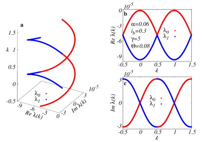
Figure 2: The two eigenvalues with the biggest real part plotted at the Riemann surface (a) and their projections to the real (b) and the imaginary (c) plane.

Having the reconstructed matrix $\mathbf{H}^{\textrm{PJ}}$ one can evaluate the rates of the even phase jumps ($2\pi n$ - PJ between the same kind of minima) using the transformations

$$\Gamma^{A}_{2n} = \intop_{-1/2}^{1/2}H_{11}^{\textrm{PJ}}e^{-ik2\pi n}dk,$$

$$\Gamma^{B}_{2n} = \intop_{-1/2}^{1/2}H_{22}^{\textrm{PJ}}e^{-ik2\pi n}dk,$$ (23)

and the odd ones between the different minima types as

$$\Gamma^{A}_{2n+1} = \intop_{-1/2}^{1/2}H_{21}^{\textrm{PJ}}e^{-ik(2\pi n+d)}dk,$$

$$\Gamma^{B}_{2n-1} = \intop_{-1/2}^{1/2}H_{12}^{\textrm{PJ}}e^{-ik(2\pi n-d)}dk.$$ (24)

This method also provides a simple tool to check its validity. The approximated mean velocity and velocity noise can be calculated directly from the rates by evaluating the formulas

$$\langle v\rangle =\lim_{\tau\rightarrow\infty}-\frac{i}{\tau}\left.\frac{\partial\mathcal{F}^{\textrm{PJ}}(k,\tau)}{\partial k}\right|_{k=0},$$ (25)

$$S =\lim_{\tau\rightarrow\infty}-\frac{1}{\tau}\left.\frac{\partial^{2}\mathcal{F}^{\textrm{PJ}}(k,\tau)}{\partial k^{2}}\right|_{k=0}.$$ (26)

These results can be compared with the mean velocity and overall noise obtained directly from the MCF method calculations [35].

III RESULTS

III.1 Strong damping

We start our analysis with the strong damping case. The main reason is that in this regime the phase dynamics is much simpler than for the intermediate and weak damping. Nevertheless, it is still far from trivial.

III.1.1 Fano factor and phase jumps

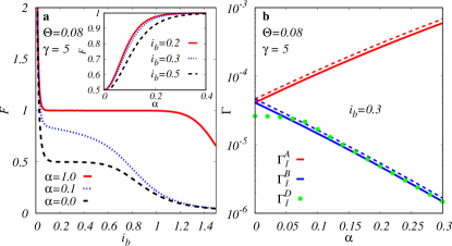
Figure 3: (a) Examples of typical low-temperature Fano factor $F=S/2\pi\langle v\rangle$ for strong damping plotted as a function of bias force for different parameters $\alpha$. The inset illustrates how the $0.5$ Fano factor plateau transits into Fano plateau with value one as $\alpha$ increase. (b) A comparison of the $\alpha$-dependence of the single-phase-jumps rates evaluated numerically (solid lines) with the analytical Kramers formula result for the overdamped case [77, 69] (dashed lines). The green bullets represent rates obtained via the simplified model where only $2\pi n$ PJ were taken into account.

In Fig. 3(a) we show the Fano factor in the strongly damped regime represented by $\gamma=5$ for three values of $\alpha$ at temperature $\Theta=0.08$. The Fano factor exhibits a characteristic divergence close to the equilibrium ($i_{b}=0$) due to the finite thermal noise. For $\alpha=0$, it follows formula $F=\frac{1}{2}\coth(\pi i_{b}/2\Theta)$ [69, Eq. (28)] for small $i_{b}$ and $\alpha=0$ with a plateau at the Poissonian value of $F=0.5$ (note that we still normalize $F$ to $2\pi$). This is in agreement with the dominant contribution to the noise from the single PJ [illustrated in Fig. 1(c)] over a distance $d=\pi$ between the equivalent neighboring minima. The situation for the finite $\alpha$ is more complicated. The range in which single PJs are the dominant source of the overall noise is not marked by a clear plateau. Rather for $0<\alpha\ll 1$ [$\alpha=0.1$ in Fig. 3(a)] we observe a slight slope in the Fano factor. This reflects the fact that for finite $\alpha$ the prevailing velocity noise contribution consists of a nontrivial combination of the single phase jumps forward over the distance of $\varphi^{B}_{m}-\varphi^{A}_{m}=d$ and backward by $\varphi^{A}_{m+1}-\varphi^{B}_{m}=2\pi-d$ [see Fig. 1(c)] where $d$ depends both on $\alpha$ and $i_{b}$. As already stated, because $d\neq\pi$ we refer to these events as the fractional phase jumps.

With increasing $\alpha$ the Fano factor increases smoothly in this region from $0.5$ signaling only PJs over the distance $\pi$ to $1$ suggesting a single PJs over $2\pi$ as shown in the inset of Fig. 3(a). Interestingly, for $\Theta=0.08$ the Fano factor approaches one even for values of $i_{b}$ that are still well below $i_{cA}$, therefore, in a regime where both minima still exist. For example, the critical current $i_{cA}$ is approximately $0.396$ at $\alpha=1$, yet its Fano factor follows the analytical result $F=\coth(\pi i_{b}/\Theta)$, valid for systems with only the first harmonic, even below this value. Nevertheless, this can be understood as a consequence of the large $\gamma$ and can be explained using the FCS method together with a simplified model of the elementary PJ processes.

Because only jumps over a single (uneven) maxima are realized in the locked state of the strong-damping case the overall dynamics of this regime can be described using just four rates: $\Gamma^{A}_{1}$ and $\Gamma^{B}_{1}$ for the forward single jumps and $\Gamma^{A}_{-1}$ and $\Gamma^{B}_{-1}$ for the backward single jumps. Moreover, the backward rates can be neglected if the bias force is strong enough. The typical dependencies of $\Gamma^{A}_{1}$ and $\Gamma^{B}_{1}$ on $\alpha$ in this regime represented by the bias force $i_{b}=0.3$ and the damping $\gamma=5$ are plotted in the Fig. 3(b) (solid lines). Both $\Gamma^{A}_{1}$ and $\Gamma^{B}_{1}$ closely follow the Kramers formula for escape across the adjacent barrier for overdamped case $\Gamma^{X}_{1}=\frac{1}{2\pi}\sqrt{|U^{\prime\prime}(\varphi^{x})|U^{\prime\prime}(\varphi^{X})}e^{-\Delta U_{X}/\Theta}$ [77, 69] (where $\Delta U_{X}=U(\varphi^{x})-U(\varphi^{X})$, and $x=a,b$; $X=A,B$) plotted with dashed lines of adequate colors. Note that because of the increasing difference $\Delta U_{B}-\Delta U_{A}$ the ratio

$$\Gamma^{A}_{1}/\Gamma^{B}_{1}\sim\exp\left[\left(\Delta U_{B}-\Delta U_{A}\right)/\Theta\right]$$ (27)

increases exponentially with $\alpha$. Consequently, for high enough $\alpha$ and low enough $\Theta$ the average waiting time for the escape from minimum $A$ $\tau_{A\rightarrow B}=1/\Gamma^{A}_{1}$ is negligible compared to the waiting time for the escape from minimum $B$ ($\tau_{B\rightarrow A}=1/\Gamma^{B}_{1}$). Therefore, in the long term, every single phase jump $B_{m-1}\rightarrow A_{m}$ is immediately followed by a single phase jump $A_{m}\rightarrow B_{m}$. The combination of these two fractional PJs is effectively a complete $2\pi$ phase jump. This is shown in Fig. 3(b) by the green bullets that were obtained via a simplified model where only the $2\pi n$ phase jumps were considered [35]

$$\Gamma^{D}_{n}=\intop\limits_{-1/2}^{1/2}\lambda_{0}(k)e^{-2\pi ikn}dk.$$ (28)

Their match with the $\Gamma^{B}_{1}$ rate for high enough $\alpha$ is consistent with the Fano-factor value of one in the inset of Fig. 3(a). This has interesting physical consequences. If the temperature is low enough, then, because $\Theta$ is in the denominator of the exponent of Eq. (27), any strongly damped $\varphi$-junction or another equivalent system describable by a double harmonic potential with a finite bias $i_{b}$ will in the steady state resemble a simple single harmonic system. As such, it can be described by the analytical formulas derived for the single-harmonic potential.

III.2 Intermediate and weak damping

The stochastic dynamics of the particle in the tilted double-well periodic potential in the regime of intermediate and weak damping is significantly richer than in the strong damping case. For example, for weak bias force, there are phase jumps over multiple maxima, and for stronger bias, a complicated switching between running and locked solutions is the prevailing source of the velocity noise. Even the retrapping of a particle from the running to locked regime has complex dynamics, as it is discussed below.

The dependencies $F-i_{b}$ for the underdamped case [plotted in Fig. 4(a)] differ qualitatively from the strongly damped case [Fig. 3(a)]. The dominant feature of the Fano factor is a huge peak [note the logarithmic scale in Fig. 4(a)] for finite $i_{b}$. As was shown in our previous study of the RCSJ model with single harmonics CPR [35], this peak is a consequence of the switching process between coexisting, but well separated, running and locked states in this range of $i_{b}$. This interpretation is also valid for the double-well potential, where, however, there exist two locked states as illustrated in Fig. 1.

We support this claim in Fig. 4(b) where an example of the stationary distribution function $W(v,\varphi)$ is plotted for the parameters (see figure description) close to the maximum of the peak. Here, the two distinct peaks at $v\approx 0$ centered around potential minima signal the two locked states. The continuous ridge that spreads above them is the running phase. In this regime, the prevailing contribution to the overall velocity noise comes from the switching between these three well-separated metastable states.

When we lower $i_{b}$ to the regime in between the thermal divergence at $i_{b}\to 0$ and the switching maximum, multiple fractional phase jumps (MPJ) become the prevailing source of the velocity noise. We now analyze the regimes of phase jumps and switching separately and then show how they transition smoothly into each other.

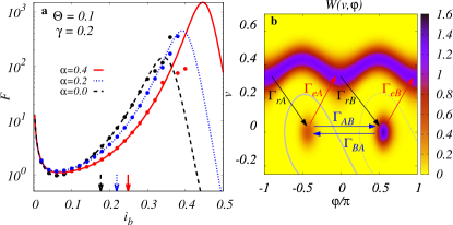
Figure 4: (a) Three examples of a typical low-temperature Fano factor $F=S/2\pi v$ dependence on the bias force for weak damping. The lines were calculated by the MCF method, and the bullets show the ME results from Eq. (26). Vertical arrows mark the related noiseless retrapping forces. (b) An illustration of the stationary distribution function $W(v,\varphi)$ in the switching regime calculated for $\gamma=0.2$, $\alpha=0.02$, $i_{b}=0.38$, and $\Theta=0.08$. The arrows illustrate the processes and their rates as used in Eq. (39). Namely, the red arrows represent escape from the locked states to the running one, the black arrows represent retrapping of the particle, and the blue arrows are the phase jumps between the locked states $A$ and $B$. The gray dashed curves show the separatrices between the running solution and the locked solution in the well $A$ (solid line) and/or well $B$ (dashed line), respectively.

III.2.1 Phase-jumps

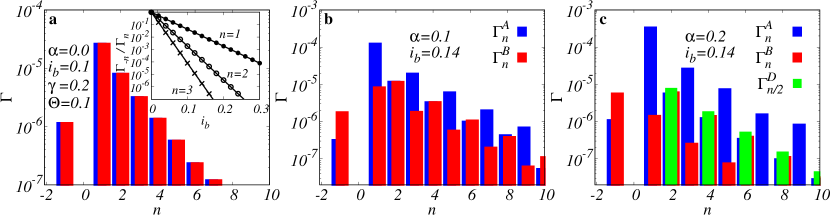
Figure 5: The rates of MPJ (of order $n$) for different values of the bias force $i_{b}$ and ratio $\alpha$. The inset in (a) is a verification of the detailed balance condition. The blue columns describe jumps starting at minimum $A$, red at minimum $B$ (a small horizontal shift is introduced for visibility), and the green columns in panel (c) show the rates obtained via the simplified model where only $2\pi n$ PJ were considered (analogously to Fig. 3(b)).

In Fig. 5 we show the rates of multiple phase jumps (MPJs) for weak damping $\gamma=0.2$, low temperature $\Theta=0.1$, and different values of $\alpha$ and $i_{b}$, where $n$ is the number of maxima bridged by a single process. The blue columns represent the rates of jumps from the minima $A$ and the red ones from the minima $B$. The $n$ dependence of the PJ rates for $\alpha=0$ shown in panel (a) is the same as that for the simple single-harmonic potential [35] up to a redefinition of the jump length. We use it as one of the tests of our extended FCS method. In the inset of Fig. 5(a) we show the ratios $\Gamma_{-n}/\Gamma_{n}$ for $n=1,\,2,\,3$ obtained numerically with FCS (bullets and crosses) and analytically from the detailed balance condition $\Gamma_{-n}/\Gamma_{n}=\exp(-\pi ni_{b}/\Theta)$ with the potential drop of $\pi i_{b}n$ along the phase jumps (lines). There is a perfect match over seven orders of magnitude for each $n=1,2,3$ proving the reliability of the FCS plus MCF method.

The profile of the rates for potentials with finite $\alpha$ is more complicated. The $n$ dependencies of the PJs rates differ qualitatively between jumps starting in different minima, as well as between odd and even $n$’s. We show this in Figs. 5(b)-(c). The rates $\Gamma_{A\,n}$ and $\Gamma_{B\,n}$ differ by several orders of magnitude for odd $n$’s [see $\alpha=0.2$ case in Fig. 5(c)], but are comparable for even $n$’s. This can be rationalized by analyzing the “trajectories” of the particular PJs following the illustrations in Fig. 1(b)(c).

The jumps $A_{m}\rightarrow A_{m+n/2}$ and $B_{m}\rightarrow B_{m+n/2}$, where $n$ is an even integer, are indeed comparable. Here, the particle had to overcome the same number of maxima $a$ as well as $b$, namely $n/2$. In the idealized case, they traveled the same distance $\pi n$. Therefore, also the related rates are equivalent. However, this is not true for odd jumps representing fractional PJs between minima of different kinds. In the case of an odd $n$ the particle overcomes $(n+1)/2$ of the lower maxima but only $(n-1)/2$ of the higher ones during a $\Gamma^{A}_{n}$ process. The opposite is true for the $\Gamma^{B}_{n}$ process. Furthermore, travel distances differ by $2\pi-2d$. Consequently, the “odd” rates differ significantly ($\Gamma^{A}_{n}\gg\Gamma^{B}_{n}$ ).

Taking into account this dynamics, the result that it is more probable for a particle to travel over $n+1$ maxima than just over $n$ [for example, $\Gamma^{A}_{3}>\Gamma^{A}_{2}$ and $\Gamma^{B}_{2}>\Gamma^{B}_{1}$ in Fig. 5(b),(c)] seems rather paradoxical. However, this is a problem of “retrapping” of a particle. Basically, if the particle has already overcome the higher maximum $b$, it will also obtain enough inertia in this regime to overcome the next lower maximum $a$. This is a parameter-dependent process, and the retrapping scenario can be rather complicated [50, 74] as is also discussed below in Sec. III.2.3.

If the single-jump rate $\Gamma^{A}_{1}$ (slip over single smaller maxima) is much larger than the rate of any other process, as is typical for high $\alpha$ and high bias force [Fig. 5(c)], it is again possible to capture the dynamics of the system using the simplified model described by Eq. (28). This is shown in Fig. 5(c), where the green columns represent the rates of the jumps $2n\pi$, where the double-well character of the potential is ignored. This model agrees well with the even rates, which do not reflect the difference between the two kinds of minima. The underlying reason is that the waiting time for an escape from the minima of type $A$ is negligible compared to other time scales.

Before moving to the switching regime, it is worth stressing that the FCS method works well up to surprisingly high Fano factors ($F\sim 10^{2}$). This is shown in Fig. 4(a) where the bullets represent the Fano factor obtained directly from the rates by Eq. (26). They are aligned with the curves obtained by the full MCF method up to the values of $i_{b}$ that are higher than the retrapping forces of the noiseless scenario [marked with the arrows at the bottom of Fig. 4(a)]. The mathematical explanation of this agreement is that for $i_{b}$ between the phase jump regime and the switching regime, the first two eigenvalues with the largest real parts are still sufficiently separated from the next ones. In addition, the comparison in Fig. 4(a) also shows that the multiple phase jumps smoothly change into the running phase as we enter the switching regime. Nevertheless, a different approach is needed to investigate the dynamics in this regime.

III.2.2 Switching processes

The phase jumps within the double well play an important role even in the regime of larger bias forces, where the switching between running and locked solutions takes place. To show this and to evaluate the escape and retrapping rates between locked and running metastable states, we again introduce a simplified model. We divide the full probability distribution function into three well-separated regions and calculate the occupation probabilities for each of them. The sharp borders between the regions are defined by separatrices of the noiseless ($\Theta=0$) dissipative steady-state solution. In plain words, we determine the momentary regime of the particle by identifying the deterministic steady state in which the particle would end with its current position and velocity for the noiseless case.

A trivial example of such a division is plotted in Fig. 4(b). There, the solid gray curve separates the $A$-valley locked state with the associated time-dependent occupation probability $P_{A}(\tau)$, the dashed curve separates the $B$-valley locked state with the associated occupation probability $P_{B}(\tau)$ and, consequently, the rest of the area belongs to the running state with occupation probability $P_{R}(\tau)$. The associated occupation probabilities are assumed to satisfy the master equation

$$\frac{d}{d\tau}\left(\begin{array}[]{c}P_{R}\\ P_{A}\\ P_{B}\end{array}\right)=\mathbf{M}^{\textrm{S}}\left(\begin{array}[]{c}P_{R}\\ P_{A}\\ P_{B}\end{array}\right),$$ (35)

with the rate matrix

$$\mathbf{M}^{\textrm{S}}=$$

$$\left(\begin{array}[]{ccc}-\left(\Gamma_{rA}+\Gamma_{rB}\right)&\Gamma_{eA}&\Gamma_{eB}\\ \Gamma_{rA}&-\left(\Gamma_{eA}+\Gamma_{AB}\right)&\Gamma_{BA}\\ \Gamma_{rB}&\Gamma_{AB}&-\left(\Gamma_{eB}+\Gamma_{BA}\right)\end{array}\right),$$ (39)

where $\Gamma_{eA}$ ($\Gamma_{eB}$) is the escape rate from potential well $A$ ($B$) to the metastable running state; $\Gamma_{rA}$ and $\Gamma_{rB}$ are the retrapping rates from metastable running state to the potential well $A$ or $B$, respectively, and $\Gamma_{AB}$ ($\Gamma_{BA}$) is the total rate of the phase jumps (of any length) from potential well $A$ to $B$ ($B$ to $A$) as it is illustrated in Fig. 4(b).

These rates can be obtained by reconstructing the switching matrix $\mathbf{M}^{\textrm{S}}=\mathbf{P}\mathbf{L}^{\textrm{S}}\mathbf{P}^{-1}$, with the diagonal matrix

$$\mathbf{L}^{\textrm{S}}=\left(\begin{array}[]{ccc}\lambda_{0}&0&0\\ 0&\lambda_{1}&0\\ 0&0&\lambda_{2}\end{array}\right)$$ (40)

containing the three eigenvalues with the largest real parts of the full Fokker-Planck operator calculated via MCF [27]. They represent the stationary state $\lambda_{0}=0$ and the first two excited states $\lambda_{1}$ and $\lambda_{2}$. The matrix $\mathbf{P}$ is a square matrix of the three related eigenvectors. The three components of each eigenvector are obtained by integrating the full MCF eigenfunctions over the areas bounded by the separatrix curves of particular solutions. The separatrices are $2\pi$ periodic and, as illustrated in Fig. 6, can be quite complex when $\gamma\to 0$. As a consequence, dynamical processes, such as the retrapping of the particle, can be very complicated [50].

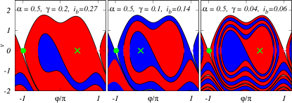
Figure 6: Separatrices (black lines) shown for different dampings and bias forces. Panels can be used to illustrate complicated retrapping dynamics of the noiseless case. Any particle within the white region will keep running forever, particles within blue and red region will get trapped following paths bounded by the regions of the same color as their initial state (they can not cross separatrix). For example, a motionless particle placed initially close to the top of the higher potential maxima, but just right to the running-locked separatrix as marked by the green bullets ($v=0,$ $\varphi=\varphi^{b}+\delta$), will end in a minima marked by the green cross.

A typical example of the rate dependencies on the bias force and related stationary occupations of particular states for $\alpha=0.2$ and $\alpha=0.02$ are plotted in Fig. 7. They represent two different regimes.

In panel (a), where $\alpha=0.2$ and $\Theta=0.1$, the phase jump from minimum $A$ to minimum $B$ has a rate $\Gamma_{AB}$ (solid blue line) that is of the same order as the escape rate $\Gamma_{eA}$ (solid red line) and much higher than the escape rate $\Gamma_{eB}$ (dashed red line) at small bias. The rate of the opposite phase jump from $B$ to $A$ (blue dashed line) is negligible. In addition, the retrapping rate $\Gamma_{rB}$ (dashed black line) is almost two orders of magnitude larger than retrapping rate $\Gamma_{rA}$ (solid black line) in the entire plotted range. This means that the mean lifetime of a particle trapped in the locked state $A$ is negligible compared to the mean lifetime of the two other states. Consequently, in the steady state, the system exhibits bistable behavior reminiscent of a system governed by a simple single-harmonic potential. This is also evident in Fig. 7(b), where the stationary occupation probabilities are plotted. For low bias forces, the particle is predominantly trapped in the state $B$, while a sharp transition to the running state is observed near the Fano factor maximum (Fig. 4, blue curve). Throughout the range depicted in the figure, the locked state $A$ exhibits minimal influence on the system dynamics.

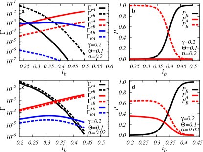
Figure 7: (a),(c) Dependencies of the escape, retrapping, and phase jump rates [illustrated in Fig. 4(b)] on the bias force within the switching regime calculated using the simplified model (35). (b),(d) Related steady-state occupation probabilities. Two qualitatively different cases are presented: panels (a) and (b) show $\alpha=0.2$ where in the steady state the system behaves effectively as a single well, and panels (c) and (d) show $\alpha=0.02$ where the double-well character is evident.

The situation is qualitatively different for $\alpha=0.02$. In this case, $\Gamma_{AB}$ and $\Gamma_{BA}$ are comparable and considerably smaller than those of the escape and retrapping processes within the range where switching occurs. However, this does not mean that phase jumps between the two locked states are irrelevant. As we discuss later in detail, it only means that their influence is apparent only on much longer timescales. At shorter ones, the phase dynamics is governed by the escape and retrapping processes. Due to the small $\alpha$, the rates of escape and retrapping processes are comparable ($\Gamma_{rA}\sim\Gamma_{rB}$ and $\Gamma_{eA}\sim\Gamma_{eB}$). Together, this leads to steady-state occupation probabilities where both locked states are relevant, as illustrated in Fig. 7(d). Interestingly, even with the low value of $\alpha=0.02$, there remains a significant difference between the occupation probabilities of states $A$ and $B$ in the steady state.

In addition to steady state, the simplified model (35) allows us to easily investigate the time evolution and to understand its particular time regimes. This can be useful not only by itself but also as a supporting tool for full-scale Langevin simulations. Let us illustrate this by investigating a retrapping process after a parameter quench.

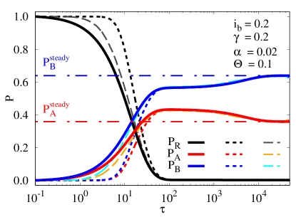
Figure 8: Example of the time dependence of the occupation probabilities of the three metastable states for $i_{b}=0.2$ with initial condition $P_{R}=1$, $P_{A}=0$ and $P_{B}=0$. This models a sudden quench of very large bias force to bias force just above the retracing force of the noiseless case. Solid lines are results of the simplified model (35), dashed lines show full Langevin simulations for two different initial conditions.

III.2.3 Retrapping

It is often difficult to reach the steady state in experimental realizations or realistic Langevin simulations. This is especially problematic for systems with low noise and weak damping. However, once we have the rates of the most relevant processes, we can investigate even long-time processes via the deterministic Eq. (35).

As an illustration, we analyze the scenario of a sudden quench of the parameters. We employ the master equation (35) and also large-scale Langevin simulations. For the latter, we used the modified Euler-Heun method LambaEulerHeun from the Julia package DifferentialEquations.jl with adaptive integration step. In the simulations, we used $\approx 6.5\times 10^{4}$ particles and, as before, their immediate regime was identified via the separatrices for the model parameters after the quench.

We focus on the case with the steady state illustrated in Fig. 7(d), i.e., $\alpha=0.02$, $\gamma=0.2$ and $\Theta=0.1$. We prepare the system in a state where it is fully running, for example, with a high bias force. For the simplified model, this means setting $P_{R}(\tau=0)=1$ and $P_{A}(\tau=0)=P_{B}(\tau=0)=0$. For the Langevin simulation, the system was first thermalized at $i_{b}=0.5$, which also gives $P_{R}(\tau=0)\approx 1$, as evident from Fig. 1. In the next step, we abruptly change the bias force to $i_{b}=0.2$, which is just below the actual retrapping force $i_{r}$. For $i_{b}=0.2$ the system is already almost exclusively in the locked steady state, yet the running state is still possible and can be identified by its separatrix.

The calculated time dependence of the occupation probabilities are shown in Fig. 8 by the solid (master equation) and dashed (Langevin dynamics) black ($P_{R}$), blue ($P_{A}$) and red ($P_{B}$) lines. The logarithmic time scale reveals several metastable regimes. At short times, there are the largest differences between the simplified model and the full simulation, as expected. In particular, the change in initial occupations is faster for the simplified model than in the simulation. This is due to the details of the initial state, that is, the initial distribution of the particles. Full dynamics starts with a relatively high mean velocity of the particles, and therefore it takes a while to slow them down.

To illustrate that this is indeed the case, we also show a simulation with different initial conditions. The dashed lines in dark gray ($P_{R}$), cyan ($P_{A}$) and orange ($P_{B}$) started in a steady state with $i_{b}=0.3$ and $\Theta=0.01$ and, therefore, significantly lower mean velocity. The short-time dynamics of this case approaches that of the simplified model. Nevertheless, the simplified model almost perfectly predicts, and, more importantly, explains, the full dynamics of these simulations at longer times.

First, particles are quickly caught in the minima around $\tau\sim 10^{1}$, because the retrapping rates are $\Gamma_{rA}\sim\Gamma_{rB}\approx 10^{-1}$. The system is close to be completely trapped before $\tau\sim 10^{2}$. However, although relatively stable, the occupation probabilities of the locked states are far from their steady-state values (horizontal dashed-dotted lines) obtained by the MCF method discussed above. This metastable state exists due to the large separation of the retrapping rates from the escape and phase jumps ones, see Fig. 7(c). Probabilities start to approach the true steady state only for $\tau\gtrsim 10^{4}$ where first the escape processes with rates $\Gamma_{eA}\sim\Gamma_{eB}\sim 10^{-4}$ and then phase jumps with $\Gamma_{AB}\sim 0.5\times 10^{-4}$ start to be relevant.

This difference of more than two orders of magnitude between the time of retrapping and reaching the steady state, as well as the existence of the metastable region, is an important observation. The long-lived metastable regime can be easily mistaken for the steady state in experiments or simulations. Furthermore, although not evident from the images presented, the Langevin simulations are becoming unstable for $\tau\sim 10^{5}$ due to the accumulation of numerical errors. The simple model does not suffer from this problem and has the benefit of being directly interpretable.

IV Conclusion

In conclusion, we have presented a theoretical study of the stochastic dynamics of a particle in the periodic double-well potential. A combination of the matrix continued fraction technique applied to solve the Fokker-Planck equation combined with the full counting statistics and simple master equation models allowed us to determine the role of particular processes in the overall dynamics.

For the strong damping, the analysis of the velocivy Fano factor revealed a region where single-phase jumps, including fractional ones, are the prevailing source of the velocity noise. We have shown that with decreasing temperature, the steady-state properties of the overdamped junction approach an effective single well system for any finite $\alpha$.

In the intermediate and weak damping regime, the FCS analyzes showed complex phase dynamics related to the single and multiple phase jumps. The revealed large differences between the rates of odd (fractional) and even phase jumps can be explained by analyzing the particle trajectories. Even in this regime we have identified parameter ranges, for which a single-harmonic analysis is sufficient for the description of the main phase slip statistics.

In the analysis of the switching regime, we have presented a simple master equation method to calculate the escape and retrapping rates. We have focused on both the regime where the double well character plays an important role in the steady state statistics and the regime where it does not. We have shown how this property is related to the retrapping, escape, and phase jump rates. We have demonstrated how these rates evolve with the bias force and determined the probabilities of steady-state occupations. The important observation is that retrapping, escape, and phase jumps can have rates that differ by orders of magnitude. This sets distinct time scales in realistic retrapping processes.

To illustrate this, we have investigated a quench, where the system in the fully running steady state is quenched to a bias force near the critical lower retrapping bias. We have shown that the results of the simplified model are in agreement with full Langevin simulations at longer times and that the differences at the short times are due to the details of the initial state used. The advantage of the simplified model is its stability at long times and, more importantly, its straightforward interpretability. Each time regime can be related to particular rates. In this way, we have been able to identify a metastable locked state, which can be easily mistaken for a steady state, due to the low escape rates and low rates of the jumps between the minima.

To wrap it up, besides providing a simple technique for analyzing the statistical properties of stochastic systems with double-well periodic potentials and analyzing their properties, we have shown two rather general features of such systems that can be crucial for the analysis of experimental setups. First, for a broad range of parameters in a strong and intermediate damping regime, the steady-state system can be approached with a simple single-harmonic model. Consequently, a two-well character of real potential can be hidden in the averaged data when the escape rate from one of the minima significantly exceeds the other rates. This can be true even for wells of similar depths at low noise.

On the other hand, the occupations of the two minima in the fully locked steady state can be significantly different even for nearly equal minima if the damping is low. In addition, these occupations are highly parameter sensitive. What is also important for analysis of experiments and numerical simulations is the realization that the retrapping time and the time when the steady-state occupation is finally reached can differ by several orders of magnitude.

Acknowledgments.— M.Ž. and T.N. acknowledge support by the Czech Science Foundation through Project No. 23-05263K. This work was supported by the Ministry of Education, Youth and Sports of the Czech Republic through the e-INFRA CZ (ID:90254). E.G. thanks Deutsche Forschungsgemeinschaft (DFG project GO-1106/6) for financial support of this collaboration. W.B. was financially supported by the Deutsche Forschungsgemeinschaft (DFG, German Research Foundation) via the SFB 1432 (project ID 425217212). M.Ž. thanks Róbert Jurčík for rewriting the code for stochastic dynamics into Julia.

References

- Likharev [1986] K. K. Likharev, Dynamics of Josephson Junctions and Circuits (Gordon and Breach, New York, 1986).
- Golubov et al. [2004] A. A. Golubov, M. Y. Kupriyanov, and E. Il’ichev, Rev. Mod. Phys. 76, 411 (2004).
- Longobardi et al. [2011] L. Longobardi, D. Massarotti, G. Rotoli, D. Stornaiuolo, G. Papari, A. Kawakami, G. P. Pepe, A. Barone, and F. Tafuri, Phys. Rev. B 84, 184504 (2011).
- Menditto et al. [2018] R. Menditto, M. Merker, M. Siegel, D. Koelle, R. Kleiner, and E. Goldobin, Phys. Rev. B 98, 024509 (2018).
- Ryabov et al. [2022] A. Ryabov, M. Žonda, and T. Novotný, Communications in Nonlinear Science and Numerical Simulation 112, 106523 (2022).
- Evstigneev et al. [2008] M. Evstigneev, O. Zvyagolskaya, S. Bleil, R. Eichhorn, C. Bechinger, and P. Reimann, Phys. Rev. E 77, 041107 (2008).
- McCann et al. [1999] L. I. McCann, M. Dykman, and B. Golding, Nature 402, 785 (1999).
- Tatarkova et al. [2003] S. A. Tatarkova, W. Sibbett, and K. Dholakia, Phys. Rev. Lett. 91, 038101 (2003).
- Čižmár et al. [2006] T. Čižmár, M. Šiler, M. Šerý, P. Zemánek, V. Garcés-Chávez, and K. Dholakia, Phys. Rev. B 74, 035105 (2006).
- Šiler et al. [2008] M. Šiler, T. Čižmár, A. Jonáš, and P. Zemánek, New. J. Phys. 10, 113010 (2008).
- Šiler and Zemánek [2010] M. Šiler and P. Zemánek, New. J. Phys. 12, 083001 (2010).
- Šiler et al. [2018] M. Šiler, L. Ornigotti, O. Brzobohatý, P. Jákl, A. Ryabov, V. Holubec, P. Zemánek, and R. Filip, Phys. Rev. Lett. 121, 230601 (2018).
- Bellando et al. [2022] L. Bellando, M. Kleine, Y. Amarouchene, M. Perrin, and Y. Louyer, Phys. Rev. Lett. 129, 023602 (2022).
- Grüner [1988] G. Grüner, Rev. Mod. Phys. 60, 1129 (1988).
- Frenken and Veen [1985] J. W. M. Frenken and J. F. v. d. Veen, Phys. Rev. Lett. 54, 134 (1985).
- Pluis et al. [1987] B. Pluis, A. W. D. van der Gon, J. W. M. Frenken, and J. F. van der Veen, Phys. Rev. Lett. 59, 2678 (1987).
- Jülicher et al. [1997] F. Jülicher, A. Ajdari, and J. Prost, Rev. Mod. Phys. 69, 1269 (1997).
- Menditto et al. [2016a] R. Menditto, H. Sickinger, M. Weides, H. Kohlstedt, D. Koelle, R. Kleiner, and E. Goldobin, Phys. Rev. E 94, 042202 (2016a).
- Hayashi et al. [2015] R. Hayashi, K. Sasaki, S. Nakamura, S. Kudo, Y. Inoue, H. Noji, and K. Hayashi, Phys. Rev. Lett. 114, 248101 (2015).
- Denisov et al. [2014] S. Denisov, S. Flach, and P. Hänggi, Physics Reports 538, 77 (2014).
- Nixon and Slater [1996] G. I. Nixon and G. W. Slater, Phys. Rev. E 53, 4969 (1996).
- Spiechowicz et al. [2016] J. Spiechowicz, J. Łuczka, and P. Hänggi, Sci. Rep. 6, 30948 (2016).
- Goychuk [2019] I. Goychuk, Phys. Rev. Lett. 123, 180603 (2019).
- Spiechowicz and Łuczka [2020] J. Spiechowicz and J. Łuczka, Phys. Rev. E 101, 032123 (2020).
- Białas et al. [2020] K. Białas, J. Łuczka, P. Hänggi, and J. Spiechowicz, Phys. Rev. E 102, 042121 (2020).
- Goychuk and Pöschel [2021] I. Goychuk and T. Pöschel, Phys. Rev. Lett. 127, 110601 (2021).
- Risken [1989] H. Risken, The Fokker-Planck Equation, 2nd ed. (Springer-Verlag, Berlin, Heidelberg, 1989).
- Elachi [1976] C. Elachi, Proceedings of the IEEE 64, 1666 (1976).
- Hänggi et al. [1990] P. Hänggi, P. Talkner, and M. Borkovec, Rev. Mod. Phys. 62, 251 (1990).
- Coffey et al. [2005] W. T. Coffey, Y. P. Kalmykov, and J. T. Waldron, The Langevin Equation With Applications to Stochastic Problems in Physics, Chemistry and Electrical Engineering, 2nd ed. (World Scientific Publishing, Singapore, 2005).
- Trahms et al. [2023] M. Trahms, L. Melischek, J. F. Steiner, B. Mahendru, I. Tamir, N. Bogdanoff, O. Peters, G. Reecht, C. B. Winkelmann, F. von Oppen, and K. J. Franke, Nature 615, 628 (2023).
- Kölzer et al. [2023] J. Kölzer, A. R. Jalil, D. Rosenbach, L. Arndt, G. Mussler, P. Schüffelgen, D. Grützmacher, H. Lüth, and T. Schäpers, Nanomaterials 13, 293 (2023).
- Žonda and Novotný [2012] M. Žonda and T. Novotný, Phys. Scripta T151 (2012).
- Gernert et al. [2014] R. Gernert, C. Emary, and S. H. L. Klapp, Phys. Rev. E 90, 062115 (2014).
- Žonda et al. [2015] M. Žonda, W. Belzig, and T. Novotný, Phys. Rev. B 91, 134305 (2015).
- Cheng and Yip [2015] L. Cheng and N. K. Yip, Physica D: Nonlinear Phenomena 297, 1 (2015).
- Wang et al. [2017] J.-Y. Wang, T.-H. Chung, T.-H. Lee, and C.-D. Chen, Sci. Rep. 7 (2017).
- Little [1967] W. A. Little, Phys. Rev. 156, 396 (1967).
- Mel’nikov [1991] V. Mel’nikov, Phys. Rep. 209, 1 (1991).
- Costantini and Marchesoni [1999] G. Costantini and F. Marchesoni, EPL 48, 491 (1999).
- Spiechowicz and Łuczka [2021] J. Spiechowicz and J. Łuczka, Phys. Rev. E 104, 024132 (2021).
- Spiechowicz et al. [2022] J. Spiechowicz, P. Hänggi, and J. Łuczka, Entropy 24, 98 (2022).
- Goldobin et al. [2007] E. Goldobin, D. Koelle, R. Kleiner, and A. Buzdin, Phys. Rev. B 76, 224523 (2007).
- Mints [1998] R. Mints, Phys. Rev. B 57, R3221 (1998).
- Mints and Papiashvili [2000] R. Mints and I. Papiashvili, Phys. Rev. B 62, 15214 (2000).
- Mints and Papiashvili [2001] R. Mints and I. Papiashvili, Phys. Rev. B 64, 134501 (2001).
- Goldobin et al. [2011] E. Goldobin, D. Koelle, R. Kleiner, and R. G. Mints, Phys. Rev. Lett. 107, 227001 (2011).
- Sickinger et al. [2012] H. Sickinger, A. Lipman, M. Weides, R. G. Mints, H. Kohlstedt, D. Koelle, R. Kleiner, and E. Goldobin, Phys. Rev. Lett. 109, 107002 (2012).
- Heim et al. [2013] D. Heim, N. Pugach, M. Kupriyanov, E. Goldobin, D. Koelle, and Kleiner, J. Phys.: Condens.Matter 25, 215701 (2013).
- Goldobin et al. [2013] E. Goldobin, R. Kleiner, D. Koelle, and R. G. Mints, Phys. Rev. Lett. 111, 057004 (2013).
- Feinberg and Balseiro [2014] D. Feinberg and C. A. Balseiro, Phys. Rev. B 90, 075432 (2014).
- Ouassou and Linder [2017] J. A. Ouassou and J. Linder, Phys. Rev. B 96, 064516 (2017).
- Jäck et al. [2017] B. Jäck, J. Senkpiel, M. Etzkorn, J. Ankerhold, C. R. Ast, and K. Kern, Phys. Rev. Lett. 119, 147702 (2017).
- Bakurskiy et al. [2017] S. V. Bakurskiy, V. I. Filippov, V. I. Ruzhickiy, N. V. Klenov, I. I. Soloviev, M. Y. Kupriyanov, and A. A. Golubov, Phys. Rev. B 95, 094522 (2017).
- Kadlecová et al. [2019] A. Kadlecová, M. Žonda, V. Pokorný, and T. Novotný, Phys. Rev. Appl. 11, 044094 (2019).
- Zhang et al. [2024] P. Zhang, A. Zarassi, L. Jarjat, V. V. de Sande, M. Pendharkar, J. S. Lee, C. P. Dempsey, A. P. McFadden, S. D. Harrington, J. T. Dong, H. Wu, A. H. Chen, M. Hocevar, C. J. Palmstrøm, and S. M. Frolov, SciPost Phys. 16, 030 (2024).
- Pal et al. [2022] B. Pal, A. Chakraborty, P. K. Sivakumar, M. Davydova, A. K. Gopi, A. K. Pandeya, J. A. Krieger, Y. Zhang, M. Date, S. Ju, N. Yuan, N. B. M. Schröter, L. Fu, and S. S. P. Parkin, Nature Physics 18, 1228 (2022).
- Souto et al. [2022] R. S. Souto, M. Leijnse, and C. Schrade, Phys. Rev. Lett. 129, 267702 (2022).
- Bartussek et al. [1994] R. Bartussek, P. Hänggi, and J. G. Kissner, EPL 28, 459 (1994).
- Hutchings et al. [2004] N. A. C. Hutchings, M. R. Isherwood, T. Jonckheere, and T. S. Monteiro, Phys. Rev. E 70, 036205 (2004).
- Hänggi and Marchesoni [2009] P. Hänggi and F. Marchesoni, Rev. Mod. Phys. 81, 387 (2009).
- Reimann [2002] P. Reimann, Phys. Rep. 361, 57 (2002).
- Kassem et al. [2017] S. Kassem, T. van Leeuwen, A. S. Lubbe, M. R. Wilson, B. L. Feringa, and D. A. Leigh, Chem. Soc. Rev. 46, 2592 (2017).
- Al-Khawaja [2008] S. Al-Khawaja, Chaos Solit. Fractals 36, 382 (2008).
- Canturk and Askerzade [2012] M. Canturk and I. N. Askerzade, J. Supercond. Nov. Magn. 26, 839 (2012).
- Baselmans et al. [1999] J. J. A. Baselmans, A. F. Morpurgo, B. J. van Wees, and T. M. Klapwijk, Nature 397, 43 (1999).
- Ferrando et al. [1992] R. Ferrando, R. Spadacini, and G. E. Tommei, Phys. Rev. A 46, R699 (1992).
- Ferrando et al. [1993] R. Ferrando, R. Spadacini, and G. E. Tommei, Phys. Rev. E 48, 2437 (1993).
- Golubev et al. [2010] D. S. Golubev, M. Marthaler, Y. Utsumi, and G. Schön, Phys. Rev. B 81, 184516 (2010).
- Vanevic et al. [2007] M. Vanevic, Y. V. Nazarov, and W. Belzig, Phys. Rev. Lett. 99 (2007), 10.1103/PhysRevLett.99.076601.
- Vanevic et al. [2008] M. Vanevic, Y. V. Nazarov, and W. Belzig, Phys. Rev. B 78 (2008), 10.1103/PhysRevB.78.245308.
- Padurariu et al. [2012] C. Padurariu, F. Hassler, and Y. V. Nazarov, Phys. Rev. B 86 (2012).
- McCumber [1968] D. E. McCumber, J. App. Phys. 39, 3113 (1968).
- Menditto et al. [2016b] R. Menditto, H. Sickinger, M. Weides, H. Kohlstedt, M. Žonda, T. Novotný, D. Koelle, R. Kleiner, and E. Goldobin, Phys. Rev. B 93, 174506 (2016b).
- Ren and Sinitsyn [2013] J. Ren and N. A. Sinitsyn, Phys. Rev. E 87, 050101 (2013).
- Li et al. [2014] F. Li, J. Ren, and N. A. Sinitsyn, EPL 105, 27001 (2014).
- Kramers [1940] H. A. Kramers, Physica 7, 284 (1940).